ANALYTICITY IN A PHENOMENOLOGY OF ELECTRO-WEAK
STRUCTURE OF HADRONS

Abstract

The utility of an application of the analyticity in a phenomenology of electro-weak structure of hadrons is demonstrated in a number of obtained new and experimentally verifiable results. With this aim first the problem of an inconsistency of the asymptotic behavior of VMD model with the asymptotic behavior of form factors of baryons and nuclei is solved generally and a general approach for determination of the lowest normal and anomalous singularities of form factors from the corresponding Feynman diagrams is reviewed. Then many useful applications by making use of the analytic properties of electro-weak form factors and amplitudes of various electromagnetic processes of hadrons are carried out.

1153 Institute of Physics, Slovak Academy of Sciences, Bratislava, Slovakia Department of Theoretical Physics, Comenius University, Bratislava, Slovakia 12 February 201019 February 2010

KEYWORDS:

1 Introduction

Up to the first half of fifties of 20th century all known elementary particles were assumed to be structureless, i.e. point-like. The latter property is reflected also in the principles of local quantum field theory (QFT) (unifying consistently quantum theory, the concept of the field and the relativistic invariance), which is considered to be a dynamical theory of elementary particle mutual interactions.

Only Hofstadter experiments [1] on elastic scattering of electrons on protons at SLAC have clearly demonstrated disagreement between theoretical expression for the cross-section calculated in the framework of the quantum electro-dynamics (QED) and the obtained experimental results. This phenomenon have revealed the non-point-like nature of the proton, which later on have been extended also to all other existing strongly interacting particles.

As a result at the calculation of the matrix element of the elastic scattering of electrons on hadrons in one-photon-exchange approximation one does not know explicitly (unlike the electron) the electromagnetic current of considered hadron to be written only symbolically and practically using various symmetries it is decomposed into maximal number of linearly independent co-variants constructed from momenta of incoming and outgoing hadrons and their spin parameters. The corresponding coefficients are scalar functions (the electromagnetic (EM) form factors (FFs)) of one variable to be chosen the squared momentum $t=q^{2}=-Q^{2}$ transferred by the virtual photon. Their number depends on the spin of the considered hadron.

Similarly can be introduced the weak FFs of hadrons, representing the contribution of the weak structure of hadrons into the dynamical quantities describing a weak interaction of hadrons in various weak processes.

A natural explanation of the electro-weak structure of hadrons was obtained only after the discovery of quark-gluon structure of strongly interacting observable particles.

The behavior of the EM FFs in the whole interval of their definition from $-\infty$ to $+\infty$ is expected to be theoretically predicted by the quantum chromo-dynamics (QCD), the gauge invariant local QFT describing mutual interactions of colored quarks and gluons. However, as it is well known, merely at sufficiently small distances (thanks to its asymptotic freedom) QCD becomes a weakly coupled quark-gluon theory to be amenable to a perturbative expansion in the running coupling constant $\alpha_{s}$ and predicts just the asymptotic behavior of FFs. In low momentum transfer region, where $\alpha_{s}$ becomes large, the quark-gluon perturbation theory breaks down and non-perturbative methods in QCD are not well worked out to give interesting results on the FFs of hadrons. The same is valid also for the low energy time-like region where FFs are complex functions of their variable and acquire the most complicated, resonant, behavior.

In such situation a phenomenological approach based on the analyticity of FFs starts to be very useful, which compensates above-mentioned problems to some extent and renders possible to achieve a line of interesting results.

In an interpretation of experimental data on EM FFs appears to be useful utilization of the analytic properties in the form of integral (so-called dispersion) relations together with the unitarity condition of FFs, which have brought the investigated FFs into relations with other FFs and amplitudes of various processes of strongly interacting particles. Such approach in the case of nucleons have led to a prediction of an existence of isoscalar and isovector vector mesons, and subsequently to the vector-meson-dominance (VMD) model [2]. The latter model is based on the assumption (to be later on experimentally confirmed in electron-positron annihilation into hadrons), that the interaction of the virtual photon with hadron is realized by a transformation of the photon to a vector meson with the same quantum numbers and then this vector meson is strongly interacting with considered hadron as in any other hadron collision.

The VMD model was revealed before the discovery of the quark model of hadrons. Despite of this fact the latter is consistent with VMD model. Really, at the energy of the photon nearly to the mass of the vector meson the latter is changed to the quark-antiquark pair, which is as a result of the confinement effect immediately bound into the vector meson with the photon quantum numbers.

Though the VMD model from the point of view of the global analysis of existing FF data has been in the past very frequently applied, it suffers from a lot of shortcomings. It does not take into account the instability of vector mesons, the unitarity condition of FFs and also the analytic properties of FFs, which could lead to a more realistic behavior of FFs in the time-like resonant region. Other serious shortcoming is the same asymptotic behavior for FFs of all hadrons, which is in contradiction with the predictions of quark model for baryons and atomic nuclei.

A solution from this situation is the universal Unitary and Analytic $(U\&A)$ model of electro-weak FFs, which is a unification of the experimental fact of a creation of unstable vector-meson resonances in the electron-positron annihilation into hadrons, the analytic properties of FFs in the complex $t$-plane and the correct asymptotic behavior of FFs as predicted by the quark model of hadrons. Its applications to many hadrons and nuclei have led to a lot of interesting results to be verifiable experimentally.

2 Electromagnetic form factors of strongly interacting particles and their properties

In this section general properties of EM FFs of strongly interacting particles, like number of FFs of the hadron under consideration, their most usual parametrization and its shortcomings, will be reviewed and subsequently resolved.

2.1 Number of electromagnetic form factors of a considered hadron

The elastic electron scattering $e^{-}h\to e^{-}h$ and the annihilations $e^{+}e^{-}\leftrightarrow h\bar{h}$, where $h$ means an arbitrary strongly interacting object (including also the atomic nucleus), are the most usual processes, in which the concept of EM FF appears. The cross-sections of these processes are proportional to the absolute value squared of the corresponding scattering amplitudes, which one knows formally to calculate in the framework of the quantum electrodynamics (QED) perturbation expansion according to the fine structure constant $\alpha\simeq 1/137$. Since the value of the fine structure constant $\alpha\ll 1$, those scattering amplitudes are considered practically in the one-photon-exchange approximation as follows

$$M(e^{-}h\to e^{-}h)\simeq M^{(\gamma)}(s,t)=e^{2}\bar{u}(k_{2})\gamma_{\mu}u(k_{1})\frac{g_{\mu\nu}}{q^{2}}\langle h|J_{\nu}^{EM}|h\rangle$$ (2.1)

and

$$M(e^{+}e^{-}\to\bar{h}h)\simeq M^{(\gamma)}(t,s)=e^{2}\bar{v}(k_{2})\gamma_{\mu}u(k_{1})\frac{g_{\mu\nu}}{q^{2}}\langle 0|J_{\nu}^{EM}|h\bar{h}\rangle,$$ (2.2)

where $g_{\mu\nu}/q^{2}$ is the photon propagator and $\langle h|J_{\nu}^{EM}|h\rangle$ (resp.$\langle 0|J_{\nu}^{EM}|h\bar{h}\rangle$) is a matrix element of the hadron EM current, which, however, due to the non-point-like nature of the hadron $h$, is unknown. Therefore, in practice it is decomposed according to a maximal number of linearly independent relativistic covariants constructed from the four-momenta and spin parameters of $h$ as follows

$$\langle h|J_{\mu}^{EM}|h\rangle=\sum_{i}R_{\mu}^{i}F_{i}(t)$$ (2.3)

or

$$\langle h\bar{h}|J_{\mu}^{EM}|0\rangle=\sum_{i}X_{\mu}^{i}F_{i}(t),$$ (2.4)

where the scalar coefficients $F_{i}(t)$ are the EM FFs of the hadron $h$ as functions of one invariant variable $t$- the momentum squared to be transferred by a virtual photon.

The number of $F_{i}(t)$ depends essentially on the spin $S$ of $h$.

Let us consider the most topical cases.

We start with the nonet of pseudoscalar mesons $\pi^{+}$, $\pi^{0}$, $\pi^{-}$, $K^{+}$, $K^{0}$, $\bar{K}^{0}$, $K^{-}$, $\eta$, $\eta^{\prime}$. Since they possess spin to be zero, for the construction of covariants $(p_{2}-p_{1})_{\mu}$ and $(p_{2}+p_{1})_{\mu}$ only two four-momenta, $p_{1}$ and $p_{2}$, are available. By an application of the gauge invariance of the EM interactions one comes to the following final parametrization

$$\langle p_{2}|J_{\mu}(0)|p_{1}\rangle=F_{P}(t)(p_{1}+p_{2})_{\mu}$$ (2.5)

only with one EM FF $F_{P}(t)$ completely describing the EM structure of any member of the nonet of pseudoscalar mesons. Moreover, making use of transformation properties of the EM current operator $J_{\mu}(x)$ and the one-particle state vector with regard to the all three discrete C, P, T transformations simultaneously, one finds the relation between particle and antiparticle FFs

$$F_{P}(t)=-F_{\bar{P}}(t)$$ (2.6)

from where it follows that for the true neutral pseudoscalar mesons $\pi^{0}$, $\eta$, $\eta^{\prime}$ the EM FFs are identically equal zero for all values from $-\infty<t<+\infty$.

The pseudoscalar meson EM FFs are normalized at $t=0$ to the charge of the considered meson.

A consideration of the nonzero value of the isospin of the pion does not enlarge a number of EM FFs and both charged pions are described by the same FF.

A completely different situation is with kaons. The $K^{+}$ and $K^{0}$ belong to the same isomultiplet with $I=1/2$. Therefore instead of the positively charged and neutral kaons one can introduce the EM current of the kaon and to investigate what isotopic structure it has. One can show, that it splits on a sum of isotopic scalar and isotopic vector. In connection with the latter the isoscalar $F^{s}_{K}(t)$ and isovector $F^{v}_{K}(t)$ FFs of the kaon are introduced to be expressed by $F_{K}^{+}(t)$ and $F_{K}^{0}(t)$ as follows

$$F^{s}_{K}(t)=\frac{1}{2}[F_{K}^{+}(t)+F_{K}^{0}(t)]$$ (2.7)

$$F^{v}_{K}(t)=\frac{1}{2}[F_{K}^{+}(t)-F_{K}^{0}(t)],$$ (2.8)

from which immediately the normalization condition

$$F^{s}_{K}(0)=F^{v}_{K}(0)=\frac{1}{2}$$ (2.9)

is obtained.

In principle, there is no problem of obtaining of the experimental information on $|F_{P}(t)|$ in $t<0$ and $t>0$ regions as $d\sigma/d\Omega\sim|F_{P}(t)|^{2}$. However, the data on nuclei (e.g $He^{4}$, $C^{12}$, $O^{16}$) exist only for $t<0$ up to now and there is no concept of the EM FF of nucleus for $t>0$ to be known by nuclear physicists.

As a consequence of a compound nature of nuclei so-called diffraction minima appear in $t<0$ region at the absolute value of their charge FF $|F_{c}(t)|$ , which are interpreted as zeros of $F_{c}(t)$ on the real axis of the complex $t$- plane. It is observed, that if more compound nucleus is investigated more diffraction minima emerge in the same range of momentum transfer values.

In the case of the octet $1/2^{+}$ baryons $p$, $n$, $\Lambda$, $\Sigma^{+}$, $\Sigma^{0}$, $\Sigma^{-}$, $\Xi^{0}$, $\Xi^{-}$ and e.g. $He^{3}$, $H^{3}$ nuclei covariants $R_{\mu}(p_{1},p_{2})$ are constructed by the four-momenta $p_{1},p_{2}$, Dirac matrices and bispinors. The final result for a parametrization of the matrix element of the EM current of the octet $1/2^{+}$ baryons takes the form

$$\langle p_{2}|J_{\mu}(0)|p_{1}\rangle=\frac{1}{2\pi^{3}}\bar{u}(p_{2})\{\gamma_{\mu}F_{1B}(t)+\frac{1}{2m_{B}}\sigma_{\mu\nu}(p_{2}-p_{1})_{\nu}F_{2B}(t)\}u(p_{1}),$$ (2.10)

where $F_{1B}(t)$ and $F_{2B}(t)$ are Dirac and Pauli FFs, respectively and $m_{B}$ is the baryon mass. From the practical point of view it is more suitable to describe the EM structure of the octet $1/2^{+}$ baryons by means of the Sachs electric $G_{EB}(t)$ and magnetic $G_{MB}(t)$ FFs, defined by the following expressions

$$G_{EB}(t)=F_{1B}(t)+\frac{t}{4m_{B}^{2}}F_{2B}(t);\quad G_{MB}(t)=F_{1B}(t)+F_{2B}(t).$$ (2.11)

There is a special coordinate system (the Breit reference frame), in which $G_{EB}(t)$ and $G_{MB}(t)$ describe a distribution of the charge and magnetic moment of the baryon. Hence they are called the electric and magnetic FFs to be normalized to the charge and magnetic moment of the baryon, respectively, for $t=0$.

Similarly to kaons, one can consider instead of the EM current of every member of the octet $1/2^{+}$ baryons the EM current of the corresponding isomultiplets and to look for their splitting into isoscalar and isovector parts. As a result one finds the following decomposition of the nucleon and $\Lambda-$, $\Sigma-$ and $\Xi-$ hyperon electric and magnetic FFs into isoscalar and isovector parts of the Dirac and Pauli FFs

$$G_{\rm Ep}(t) = [F_{1N}^{\rm s}(t)+F_{1N}^{\rm v}(t)]+\frac{t}{4m^{2}_{p}}[F_{2N}^{\rm s}(t)+F_{2N}^{\rm v}(t)]$$ (2.12)

$$G_{\rm Mp}(t) = [F_{1N}^{\rm s}(t)+F_{1N}^{\rm v}(t)]+[F_{2N}^{\rm s}(t)+F_{2N}^{\rm v}(t)]$$

$$G_{\rm En}(t) = [F_{1N}^{\rm s}(t)-F_{1N}^{\rm v}(t)]+\frac{t}{4m^{2}_{n}}[F_{2N}^{\rm s}(t)-F_{2N}^{\rm v}(t)]$$ (2.13)

$$G_{\rm Mn}(t) = [F_{1N}^{\rm s}(t)-F_{1N}^{\rm v}(t)]+[F_{2N}^{\rm s}(t)-F_{2N}^{\rm v}(t)]$$

$$G_{\rm E\Lambda}(t) = F_{1\Lambda}^{\rm s}(t)+\frac{t}{4m^{2}_{\Lambda}}F_{2\Lambda}^{\rm s}(t)$$

$$G_{\rm M\Lambda}(t) = F_{1\Lambda}^{\rm s}(t)+F_{2\Lambda}^{\rm s}(t)$$ (2.14)

$$G_{\rm E\Sigma^{+}}(t) = [F_{1\Sigma}^{\rm s}(t)+F_{1\Sigma}^{\rm v}(t)]+\frac{t}{4m^{2}_{\Sigma^{+}}}[F_{2\Sigma}^{\rm s}(t)+F_{2\Sigma}^{\rm v}(t)]$$

$$G_{\rm M\Sigma^{+}}(t) = [F_{1\Sigma}^{\rm s}(t)+F_{1\Sigma}^{\rm v}(t)]+[F_{2\Sigma}^{\rm s}(t)+F_{2\Sigma}^{\rm v}(t)]$$

$$G_{\rm E\Sigma^{0}}(t) = F_{1\Sigma}^{\rm s}(t)+\frac{t}{4m^{2}_{\Sigma^{0}}}F_{2\Sigma}^{\rm s}(t)$$

$$G_{\rm M\Sigma^{0}}(t) = F_{1\Sigma}^{\rm s}(t)+F_{2\Sigma}^{\rm s}(t)$$ (2.15)

$$G_{\rm E\Sigma^{-}}(t) = [F_{1\Sigma}^{\rm s}(t)-F_{1\Sigma}^{\rm v}(t)]+\frac{t}{4m^{2}_{\Sigma^{-}}}[F_{2\Sigma}^{\rm s}(t)-F_{2\Sigma}^{\rm v}(t)]$$

$$G_{\rm M\Sigma^{-}}(t) = [F_{1\Sigma}^{\rm s}(t)-F_{1\Sigma}^{\rm v}(t)]+[F_{2\Sigma}^{\rm s}(t)-F_{2\Sigma}^{\rm v}(t)]$$

$$G_{\rm E\Xi^{0}}(t) = [F_{1\Xi}^{\rm s}(t)+F_{1\Xi}^{\rm v}(t)]+\frac{t}{4m^{2}_{\Xi^{0}}}[F_{2\Xi}^{\rm s}(t)+F_{2\Xi}^{\rm v}(t)]$$

$$G_{\rm M\Xi^{0}}(t) = [F_{1\Xi}^{\rm s}(t)+F_{1\Xi}^{\rm v}(t)]+[F_{2\Xi}^{\rm s}(t)+F_{2\Xi}^{\rm v}(t)]$$ (2.16)

$$G_{\rm E\Xi^{-}}(t) = [F_{1\Xi}^{\rm s}(t)-F_{1\Xi}^{\rm v}(t)]+\frac{t}{4m^{2}_{\Xi^{-}}}[F_{2\Xi}^{\rm s}(t)-F_{2\Xi}^{\rm v}(t)]$$

$$G_{\rm M\Xi^{-}}(t) = [F_{1\Xi}^{\rm s}(t)-F_{1\Xi}^{\rm v}(t)]+[F_{2\Xi}^{\rm s}(t)-F_{2\Xi}^{\rm v}(t)].$$

The experimental information on $G_{EB}(t)$, $G_{MB}(t)$ in $t<0$ region can be easily determined from parameters of the straight-line (so-called Rosenbluth) plot of

$$\frac{d\sigma(e^{-}B\to e^{-}B)}{d\Omega}/\left\{\frac{\alpha^{2}\cos^{2}(\vartheta/2)}{4E^{2}\sin^{4}(\vartheta/2)[1+(2E/m_{B})\sin^{2}(\vartheta/2)]}\right\}=$$ (2.17)

$$= A(t)+B(t)\tan^{2}(\theta/2),$$

where

$$A(t) = \frac{G^{2}_{EB}(t)-\frac{t}{4m_{B}^{2}}G^{2}_{MB}(t)}{1-\frac{t}{4m_{B}^{2}}},$$

$$B(t) = -2\frac{t}{4m_{B}^{2}}G^{2}_{MB}(t)$$ (2.18)

in the laboratory system versus $\tan^{2}(\vartheta/2)$ at fixed $t$ and for nuclei again diffraction minima appear.

Till now all existing data on $G_{EB}(t)$, $G_{MB}(t)$ in $t>0$ region are obtained from $\sigma_{tot}(e^{+}e^{-}\leftrightarrow B\bar{B})$ under the assumption that $|G_{EB}(t)|=|G_{MB}(t)|$.

The covariants $R_{\mu}(p_{1},p_{2})$ for EM FFs of the nonet of vector mesons, $\rho^{+}$, $\rho^{0}$, $\rho^{-}$, $K^{*+}$, $K^{*0}$, $\bar{K}^{*0}$, $K^{*-}$, $\omega$, $\Phi$ and also of the deuteron are constructed by the four-momenta $p_{1}$, $p_{2}$ and polarization vectors. Then a parametrization of the matrix element of the EM current of vector-particles takes the following form

$$\langle p_{2}|J_{\mu}^{EM}|p_{1}\rangle=F_{1}(t)(\xi^{\prime*}\cdot\xi)d_{\mu}+F_{2}(t)[\xi_{\mu}(\xi^{\prime*}\cdot q)-\xi_{\mu}^{\prime*}(\xi\cdot q)]-F_{3}(t)\frac{(\xi\cdot q)(\xi^{\prime*}\cdot q)}{2m_{V}^{2}}d_{\mu},$$ (2.19)

where $\xi$ and $\xi^{\prime}$ are polarization vectors for incoming and outgoing particles of four-momenta $p_{1}$ and $p_{2}$, respectively

$$\xi^{\prime}\cdot p_{2}=0;\quad\xi\cdot p_{1}=0;\quad\xi^{\prime 2}=-1;\quad\xi^{2}=-1;$$

$$d_{\mu}=(p_{2}+p_{1})_{\mu};\quad q_{\mu}=(p_{2}-p_{1})_{\mu}.$$

Practically, it is convenient to describe the EM structure of vector particles by an analogue of the Sachs FFs of nucleons

$$G_{C}(t) = F_{1}(t)-\frac{t}{6m_{H}^{2}}G_{Q}(t);\quad G_{M}(t)=F_{2}(t);$$

$$G_{Q}(t) = F_{1}(t)-F_{2}(t)+(1-\frac{t}{4m_{H}^{2}})F_{3}(t)$$ (2.20)

the names of which, the charge $G_{C}(t)$, the magnetic $G_{M}(t)$ and the quadrupole $G_{Q}(t)$ FFs, are derived from the fact that their static values correspond to the charge, magnetic and quadrupole moment of the vector particles.

One can determine all $G_{C}(t)$, $G_{M}(t)$, $G_{Q}(t)$ FFs from $d\sigma/d\Omega$ of the $e^{-}V\to e^{-}V$ process provided that polarized particles are used in the corresponding experiments. Otherwise only the elastic structure functions $A(t)$ and $B(t)$ can be drawn out from

$$\frac{d\sigma}{d\Omega}=\frac{\alpha^{2}E^{\prime}\cos^{2}(\vartheta/2)}{4E^{3}\sin^{4}(\vartheta/2)}[A(t)+B(t)\tan^{2}(\vartheta/2)],$$ (2.21)

where

$$A(t) = -\frac{t}{6m_{V}^{2}}(1-\frac{t}{4m_{V}^{2}})G_{M}^{2}(t)+G_{C}^{2}(t)+\frac{t^{2}}{18m_{V}^{4}}G_{Q}^{2}(t)$$

$$B(t) = -\frac{t}{3m_{V}^{2}}(1-\frac{t}{4m_{V}^{2}})^{2}G_{M}^{2}(t).$$ (2.22)

On the other hand, from

$$\sigma_{tot}(e^{+}e^{-}\to V\bar{V})=\frac{\pi\alpha^{2}\beta^{3}_{V}}{3t}\left\{3|G_{C}(t)|^{2}+\frac{t}{m_{V}^{2}}\left[|G_{M}(t)|^{2}+\frac{1}{6m_{V}^{2}}|G_{Q}(t)|^{2}\right]\right\}$$ (2.23)

one can see immediately that it is not a single task to obtain any experimental information on the corresponding EM FFs in $t>0$ region.

For strongly interacting particles $h$ with $S>1$ a situation is even more complicated and generally it is not solved up to now.

2.2 Properties of electromagnetic form factors of hadrons

Summarizing our knowledge about the experimental behavior of EM FFs we come to a conclusion, that all of them have a similar behavior in the shape. But they differ in the asymptotic behavior, normalization, number of bumps corresponding to vector-meson resonances and also in the shape and height of those bumps.

A behavior of EM FFs is a matter of predictions of a strong interaction dynamical theory. However, there is no such theory able to predict a correct behavior of $|F_{h}(t)|$ for $-\infty<t<+\infty$ up to now and only partial successes were achieved in this direction.

The great discovery in the elementary particle physics was a revelation of the quark-gluon structure of hadrons and its direct relation [3, 4] to the asymptotic behavior of EM FFs to be determined by a number of constituent quarks $n_{q}$ of the hadron $h$ as follows

$$F_{h}(t)_{|t|\to\infty}\sim t^{1-n_{q}},$$ (2.24)

which is in a qualitative agreement with existing experimental data.

On the other hand, it is well known that on the role of a true dynamical theory of strong interactions QCD, the gauge-invariant local quantum field theory of interactions of quarks and gluons, is pretending. But, as a consequence of the asymptotic freedom of QCD, in the framework of the perturbation theory, the latter is able to reproduce [5, 6, 7] just the asymptotic behavior (2.24) up to logarithmic corrections.

Not even the nonperturbative QCD sum rules [8] by means of which a prediction [9, 10] of a behavior of EM FFs in a restricted $t<0$ region is achieved, solve the problem of a reconstruction of EM FFs in the framework of QCD completely.

For a completeness we mention also the chiral perturbation approach [11], in the framework of which a correct behavior of EM FFs of hadrons around the point $t=0$ is predicted. This is very important to be mentioned as the chiral perturbation approach is equivalent to QCD at low energies where the running coupling constant $\alpha_{s}(t)$ takes large values and the PQCD is nonapplicable.

Summarizing, QCD (not even its equivalent form) gives no quantitative predictions in the most important part of the time-like ($4m^{2}_{\pi}<t\leq 4GeV^{2}$) region, where EM FFs are already complex functions of $t$ and the $e^{+}e^{-}$ annihilation experiments exhibit a nontrivial behavior of measured cross-sections caused by a creation of various unstable vector-meson states.

Therefore for the present an appropriate phenomenological approach based on the synthesis of the experimental fact of a creation of vector-mesons in $e^{+}e^{-}$- annihilation processes into hadrons, the asymptotic behavior (2.24) and the well-established analytic properties, leading to the U&A model of EM structure of strongly interacting particles, is still the most successful way in a global theoretical reconstruction of EM FFs of hadrons.

The vector-meson creation in $e^{+}e^{-}$- annihilation processes into hadrons is taken into account by means of the vector-meson-dominance (VMD) model given for isoscalar and isovector parts of EM FFs by the relation

$$F_{h}^{s,v}(t)=\sum_{V=1}^{n}\frac{m^{2}_{V}}{(m^{2}_{V}-t)}(f_{Vh\bar{h}}/f_{V})$$ (2.25)

where $f_{Vh\bar{h}}$ and $f_{V}$ are the vector-meson-hadron and the universal vector-meson coupling constants, respectively, and $m_{V}$ is the vector-meson mass.

The analyticity consists in a hypothesis that all EM FFs are analytic functions in the whole complex $t$- plane besides infinite number of branch points on the positive real axis corresponding to normal and anomalous thresholds.

2.3 Vector-meson-dominance model for form factors of hadrons

There are experimentally confirmed neutral vector-mesons [12] with quantum numbers to be identical with photon. They have the isospin either 0 or 1.

On the other hand the EM current of hadrons is by a rotation in the isospin-space transformed like the sum of isotopic scalar and the third component of isotopic vector. The latter transformation properties reflect well known fact of the non-conservation of the isospin in the EM interactions and lead automatically to a phenomenon, observed experimentally, that at the absorption and creation of virtual photon by hadron the isospin value can be changed by 1. Therefore the photon can be considered to be a superposition of states with isospin value 0 (the isoscalar photon) and isospin value 1 (the isovector photon). Then neutral vector-mesons with quantum numbers $J^{PC}=1^{--}$ differ from the photon only by the mass and there is no obstacle to assume that there are between virtual photons and vector-mesons transitions with a definite probability determined by the coupling constant

$$g_{\gamma{\rm V}}=e\frac{m^{2}_{\rm V}}{f_{\rm V}},$$ (2.26)

where $e$ is the electric charge , $m_{\rm V}$ is the mass of vector-meson and $f_{V}$ is the so-called universal vector-meson coupling constant.

The transition of virtual photons to neutral vector mesons is confirmed practically by the neutral vector-meson decay into lepton-antilepton pair. Really, if we assume the transition $\gamma\leftrightarrow V^{0}$, then the $V^{0}\to\ell^{+}\ell^{-}$ decay can be explained as a result of a change of $V^{0}$ into virtual photon $\gamma^{*}$ which subsequently is creating the lepton-antilepton pair (Fig. 2.1).

Figure 2.1: Decay of neutral vector meson into lepton pair.

It seems to be natural a generalization of this mechanism to any process of an interaction of photon with hadron, in which first the photon is changed to vector-meson and then the latter is interacting with the hadron like in other hadron collisions by strong interactions.

In conformity with the idea of VMD model any EM FF of hadron in the first approximation can be represented by a sum of Feynman diagrams with and exchange of vector-mesons $V^{0}$ (Fig. 2.2).

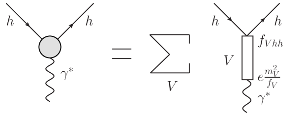
Figure 2.2: Approximation of hadron FF by a sum of VMD terms.

By an application of standard methods of quantum field theory to an explicit calculation of contributions of this sum of Feynman diagrams one obtains

$$eF_{h}(t)=\sum_{\rm V}\frac{(g_{\gamma{\rm V}}.f_{{\rm V}h\bar{h}})}{m^{2}_{\rm V}-t}$$ (2.27)

the VMD parametrization (in the zero width, i.e. $\Gamma_{\rm V}=0$ approximation) of the hadron EM FF, which is, taking into account also the relation (2.26), normalized for $t=0$ in the form

$$F_{h}(0)=\sum_{\rm V}(f_{{\rm V}h\bar{h}}/f_{\rm V})$$ (2.28)

and it possess the asymptotic behavior

$$F_{h}(t)\sim t^{-1}_{|t|\to\infty}$$ (2.29)

to be the same for EM FFs of all strongly interacting particles.

The relation (2.26) can be derived by taking, first the expression (2.27) for the pion FF, the isovector part of the kaon FF and the isovector part of the Dirac nucleon FF to be saturated by only the lowest vector-meson, the $\rho$-meson. As a result one can write the following three independent expressions

$$eF_{\pi}(t)=\frac{g_{\gamma\rho}.f_{\rho\pi\pi}}{m^{2}_{\rho}-t}$$ (2.30)

$$eF^{v}_{K}(t)=\frac{g_{\gamma\rho}.f_{\rho K\bar{K}}}{m^{2}_{\rho}-t}$$ (2.31)

$$eF^{v}_{1N}(t)=\frac{g_{\gamma\rho}.f^{1}_{\rho N\bar{N}}}{m^{2}_{\rho}-t}$$ (2.32)

in which the normalization condition at $t=0$ gives

$$e=\frac{g_{\gamma\rho}.f_{\rho\pi\pi}}{m^{2}_{\rho}}$$ (2.33)

$$\frac{e}{2}=\frac{g_{\gamma\rho}.f_{\rho K\bar{K}}}{m^{2}_{\rho}}$$ (2.34)

$$\frac{e}{2}=\frac{g_{\gamma\rho}.f^{1}_{\rho N\bar{N}}}{m^{2}_{\rho}}.$$ (2.35)

By a multiplication of the last two equations by 2, one can obtain the following universal interaction of the $\rho$-meson to be expressed by the relations

$$f_{\rho\pi\pi}=2f_{\rho K\bar{K}}=2f^{1}_{\rho N\bar{N}}=f_{\rho},$$ (2.36)

where the coupling constant $f_{\rho}$ is named to be the universal coupling constant of the $\rho$-meson and the coupling constant of the $\rho$-meson with the virtual photon $g_{\gamma\rho}$ can be written as follows

$$g_{\gamma\rho}=e\frac{m^{2}_{\rho}}{f_{\rho}}.$$ (2.37)

Generalization of the previous relation to any other vector meson V with quantum numbers of the photon leads to the form of (2.26).

2.4 Asymptotic conditions for form factors represented by VMD model

As we have noticed above, from one side the quark model of hadrons predicts (2.24) the asymptotic behavior of EM FF of hadron to be dependent, in conformity with existing experimental data, on the number of constituent quarks of considered hadron.

On the other hand, the VMD model for EM FFs (2.3) of strongly interacting particles gives the same asymptotic behavior (2.29) independently on the number of constituent quarks.

This conflict is solved in this paragraph [13] by a derivation of the so-called asymptotic conditions. However, there are known in practice two seemingly different asymptotic conditions. Further we clearly demonstrate their equivalence.

Generally, let us assume that the FF in (2.25) is saturated by $n$ different vector meson pole terms and it has to have the asymptotic behavior

$$F_{h}(t)_{|t|\to\infty}\sim t^{-m},$$ (2.38)

where $m\leq n$.

Transforming the VMD pole representation (2.25) into a common denominator one obtains FF in the form of a rational function with a polynomial of $(m-1)$ degree

$$P_{n-1}(t)=A_{0}+A_{1}\cdot t+A_{2}\cdot t^{2}+\cdots+A_{n-1}\cdot t^{n-1}$$ (2.39)

in the numerator, where

$$A_{n-1} = (-1)^{n-1}\sum_{j=1}^{n}m_{j}^{2}a_{j}$$

$$A_{n-2} = (-1)^{n-2}\sum_{i=1\atop i\neq j}^{n}m_{i}^{2}\sum_{j=1}^{n}m_{j}^{2}a_{j}$$

$$A_{n-3} = (-1)^{n-3}\sum_{i_{1},i_{2}=1\atop i_{1}<i_{2},i_{r}\neq j}^{n}m_{i_{1}}^{2}m_{i_{2}}^{2}\sum_{j=1}^{n}m_{j}^{2}a_{j}$$

$$A_{n-4} = (-1)^{n-4}\sum_{i_{1},i_{2},i_{3}=1\atop i_{1}<i_{2}<i_{3},i_{r}\neq j}^{n}m_{i_{1}}^{2}m_{i_{2}}^{2}m_{i_{3}}^{2}\sum_{j=1}^{n}m_{j}^{2}a_{j}$$

………

$$A_{n-(m-1)} = (-1)^{n-m+1}\sum_{i_{1},i_{2},\cdots i_{m-2}=1\atop i_{1}<i_{2}\cdots<i_{m-2},i_{r}\neq j}^{n}m_{i_{1}}^{2}m_{i_{2}}^{2}\cdots m_{i_{m-2}}^{2}\sum_{j=1}^{n}m_{j}^{2}a_{j}$$ (2.40)

$$A_{n-m} = (-1)^{n-m}\sum_{i_{1},i_{2},\cdots i_{m-1}=1\atop i_{1}<i_{2}\cdots<i_{m-1},i_{r}\neq j}^{n}m_{i_{1}}^{2}m_{i_{2}}^{2}\cdots m_{i_{m-2}}^{2}m_{i_{m-1}}^{2}\sum_{j=1}^{n}m_{j}^{2}a_{j}$$

………

$$A_{2} = (-1)^{2}\sum_{i_{1},i_{2},\cdots i_{n-3}=1\atop i_{1}<i_{2}\cdots<i_{n-3},i_{r}\neq j}^{n}m_{i_{1}}^{2}m_{i_{2}}^{2}\cdots m_{i_{n-3}}^{2}\sum_{j=1}^{n}m_{j}^{2}a_{j}$$

$$A_{1} = (-1)\sum_{i_{1},i_{2},\cdots i_{n-2}=1\atop i_{1}<i_{2}\cdots<i_{n-2},i_{r}\neq j}^{n}m_{i_{1}}^{2}m_{i_{2}}^{2}\cdots m_{i_{n-3}}^{2}m_{i_{n-2}}^{2}\sum_{j=1}^{n}m_{j}^{2}a_{j}$$

$$A_{0} = \sum_{i_{1},i_{2},\cdots i_{n-1}=1\atop i_{1}<i_{2}\cdots<i_{n-1},i_{r}\neq j}^{n}m_{i_{1}}^{2}m_{i_{2}}^{2}\cdots m_{i_{n-2}}^{2}m_{i_{n-1}}^{2}\sum_{j=1}^{n}m_{j}^{2}a_{j}$$

and $a_{j}=(f_{jhh}/f_{j})$.

In order to achieve the assumed asymptotic behavior (2.38) one requires in (2.39) the first $(m-1)$ coefficients from the highest powers of $t$ to be zero and as a result the following first system of linear homogeneous algebraic equations for the coupling constant ratios is obtained

$$\sum\limits_{j=1}^{n} m_{j}^{2}a_{j}=0$$

$$\sum\limits_{i=1\atop i\neq j}^{n} m_{i}^{2}\sum_{j=1}^{n}m_{j}^{2}a_{j}=0$$

$$\sum\limits_{i_{1},i_{2}=1\atop i_{1}<i_{2},i_{r}\neq j}^{n} m_{i_{1}}^{2}m_{i_{2}}^{2}\sum_{j=1}^{n}m_{j}^{2}a_{j}=0$$

$$\sum\limits_{i_{1},i_{2},i_{3}=1\atop i_{1}<i_{2}<i_{3},i_{r}\neq j}^{n} m_{i_{1}}^{2}m_{i_{2}}^{2}m_{i_{3}}^{2}\sum_{j=1}^{n}m_{j}^{2}a_{j}=0$$

………

$$\sum\limits_{i_{1},i_{2},\cdots i_{m-2}=1\atop i_{1}<i_{2}\cdots<i_{m-2},i_{r}\neq j}^{n} m_{i_{1}}^{2}m_{i_{2}}^{2}\cdots m_{i_{m-2}}^{2}\sum\limits_{j=1}^{n}m_{j}^{2}a_{j}=0.$$

As one can see from (2.4) with increased $m$ the coefficients become sums of more and more complicated products of squared vector-meson masses.

For a derivation of the second system we employ the assumed analytic properties of EM FFs of hadrons, consisting of infinite number of branch points on the positive real axis, i.e. cuts. The first cut extends from the lowest branch point $t_{0}$ to $+\infty$. Then one can apply the Cauchy theorem to FF in $t$- plane

$$\frac{1}{2\pi i}\oint F_{h}(t)dt=0$$ (2.42)

where the closed integration path consists of the circle $C_{R}$ of the radius $R\to\infty$ and the path avoiding the cut on the positive real axis. As a result (2.42) can be rewritten into a sum of the following four integrals

$$\frac{1}{2\pi i}\left\{\int_{C_{R}}F_{h}(t)dt+\int_{+\infty}^{t_{0}}F_{h}(t-i\epsilon)dt+\int_{C_{r}/2}F_{h}(t)dt+\int^{+\infty}_{t_{0}}F_{h}(t+i\epsilon)dt\right\}=0$$ (2.43)

where $\epsilon\ll 1$ and $C_{r}/2$ is the half-circle joining the upper boundary of the cut with the lower-boundary of the cut around the lowest branch point $t_{0}$. The contribution of the first integral in (2.43) is zero as $F_{h}(t)$ for $R\to\infty$ is vanishing. One can prove also that the third integral in (2.43) for $r\to 0$ is zero. As a result one gets

$$\frac{1}{2\pi i}\int_{t_{0}}^{\infty}[F_{h}(t+i\epsilon)-F_{h}(t-i\epsilon)]dt=0.$$ (2.44)

Then, taking into account the reality condition of FF

$$F_{h}^{*}(t)=F_{h}(t^{*})$$ (2.45)

following from the general Schwarz reflection principle in the theory of analytic functions, one arrives at the integral superconvergent sum rule

$$\frac{1}{\pi}\int_{t_{0}}^{\infty}ImF_{h}(t)dt=0$$ (2.46)

for the imaginary part of the FF under consideration.

Repeating the same procedure for the functions $tF_{h}(t)$, $t^{2}F_{h}(t)$, $\cdots$, $t^{m-2}F_{h}(t)$ which possess the same analytic properties in the complex $t$-plane as $F_{h}(t)$, one gets another $(m-2)$ superconvergent sum rules

$$\frac{1}{\pi}\int_{t_{0}}^{\infty}t\cdot ImF_{h}(t)dt = 0$$

$$\frac{1}{\pi}\int_{t_{0}}^{\infty}t^{2}\cdot ImF_{h}(t)dt = 0$$ (2.47)

$$\ldots\ldots\ldots$$

$$\frac{1}{\pi}\int_{t_{0}}^{\infty}t^{m-2}\cdot ImF_{h}(t)dt=0.$$

Now, approximating the FF imaginary part by $\delta$- function in the following form

$$ImF(t)=\pi\sum_{i}^{n}a_{i}\delta(t-m_{i}^{2})m_{i}^{2}$$ (2.48)

and substituting it into (2.46) and (2.47) one obtains the second system of $(m-1)$ linear homogeneous algebraic equations for coupling constant ratios $a_{i}=(f_{ihh}/f_{i})$

$$\sum_{i=1}^{n}m_{i}^{2}a_{i}=0$$

$$\sum_{i=1}^{n}m_{i}^{4}a_{i}=0$$

$$\sum_{i=1}^{n}m_{i}^{6}a_{i}=0$$ (2.49)

………

$$\sum_{i=1}^{n}m_{i}^{2(m-2)}a_{i}=0$$

$$\sum_{i=1}^{n}m_{i}^{2(m-1)}a_{i}=0,$$

where coefficients are simply even powers of the vector-meson masses.

Further we demonstrate explicitly that both systems of the algebraic equations, (2.4) and (2.49), are equivalent, despite the fact that they have been derived starting from different properties of the EM FF, and thus they appear to be different.

We start with the equations (2.4). From a direct comparison of systems (2.4) and (2.49) one can see immediately the identity of the first equations in them.

The second equation in (2.4) can be written explicitly as follows

$$(m_{2}^{2}+m_{3}^{2}+\cdots+m_{n}^{2})m_{1}^{2}a_{1}+(m_{1}^{2}+m_{3}^{2}+\cdots+m_{n}^{2})m_{2}^{2}a_{2}+\cdots+$$ (2.50)

$$+ (m_{1}^{2}+m_{2}^{2}+\cdots+m_{n-1}^{2})m_{n}^{2}a_{n}=0.$$

Adding and subtracting $m_{1}^{4}a_{1}$ to the first term of the sum, $m_{2}^{4}a_{2}$ to the second term of the sum $\cdots$ etc. and finally $m_{n}^{4}a_{n}$ to the last term of the sum, the equation (2.50) can be modified into the form

$$\sum_{i=1}^{n}m_{i}^{2}\sum_{j=1}^{n}m_{j}^{2}a_{j}-\sum_{j=1}^{n}m_{j}^{4}a_{j}=0,$$ (2.51)

from where one can see immediately that the second equation in (2.49) is fulfilled

$$\sum_{j=1}^{n}m_{j}^{4}a_{j}=0$$ (2.52)

as $\sum_{j=1}^{n}m_{j}^{2}a_{j}=0$ is just the first equation in (2.4) and (2.49) as well.

The third equation in (2.4) can be written explicitly as follows

$$(m^{2}_{2}m_{3}^{2}+m^{2}_{2}m_{4}^{2}+\cdots+m^{2}_{2}m_{n}^{2}+m^{2}_{3}m_{4}^{2}+m^{2}_{3}m_{5}^{2}+\cdots$$

$$+ m^{2}_{3}m_{n}^{2}+\cdots+m^{2}_{n-1}m_{n}^{2})m_{1}^{2}a_{1}+$$

$$+ (m^{2}_{1}m_{3}^{2}+m^{2}_{1}m_{4}^{2}+\cdots+m^{2}_{1}m_{n}^{2}+m^{2}_{3}m_{4}^{2}+m^{2}_{3}m_{5}^{2}+\cdots$$

$$+ m^{2}_{3}m_{n}^{2}+\cdots+m^{2}_{n-1}m_{n}^{2})m_{2}^{2}a_{2}+$$

$$+ (m^{2}_{1}m_{2}^{2}+m^{2}_{1}m_{4}^{2}+\cdots+m^{2}_{1}m_{n}^{2}+m^{2}_{2}m_{4}^{2}+m^{2}_{2}m_{5}^{2}+\cdots$$

$$+ m^{2}_{2}m_{n}^{2}+\cdots+m^{2}_{n-1}m_{n}^{2})m_{3}^{2}a_{3}+$$

………

$$+ (m^{2}_{1}m_{2}^{2}+m^{2}_{1}m_{3}^{2}+\cdots+m^{2}_{1}m_{n-2}^{2}+m^{2}_{1}m_{n}^{2}+m^{2}_{2}m_{3}^{2}+\cdots$$

$$+ m^{2}_{2}m_{n-2}^{2}+m^{2}_{2}m_{n}^{2}\cdots+$$

$$+ m^{2}_{n-2}m_{n}^{2})m_{n-1}^{2}a_{n-1}+$$

$$+ (m^{2}_{1}m_{2}^{2}+m^{2}_{1}m_{3}^{2}+\cdots+m^{2}_{1}m_{n-2}^{2}+m^{2}_{1}m_{n-1}^{2}+m^{2}_{2}m_{3}^{2}+\cdots$$

$$+ m^{2}_{2}m_{n-2}^{2}+m^{2}_{2}m_{n-1}^{2}+$$

$$+ \cdots+m^{2}_{n-2}m_{n-1}^{2})m_{n}^{2}a_{n}=0.$$

Now adding and subtracting all missing terms in (2.4) from $\sum_{{i_{1}},{i_{2}}=1\atop{i_{1}}<{i_{2}}}^{n}m_{i_{1}}^{2}m_{i_{2}}^{2}\sum_{j=1}^{n}m_{j}^{2}a_{j}$ which in the substraction form can be written explicitly as follows

$$- (m_{2}^{2}+m_{3}^{2}+m_{4}^{2}+\cdots m_{n}^{2})m_{1}^{4}a_{1}-$$ (2.54)

$$- (m_{1}^{2}+m_{3}^{2}+m_{4}^{2}+\cdots m_{n}^{2})m_{2}^{4}a_{2}-$$

$$- (m_{1}^{2}+m_{2}^{2}+m_{4}^{2}+\cdots m_{n}^{2})m_{3}^{4}a_{3}-$$

………

$$- (m_{1}^{2}+m_{2}^{2}+\cdots+m_{n-2}^{2}+m_{n}^{2})m_{n-1}^{4}a_{n-1}-$$

$$- (m_{1}^{2}+m_{2}^{2}+\cdots+m_{n-2}^{2}+m_{n-1}^{2})m_{n}^{4}a_{n}$$

and again subtracting and adding $m_{1}^{6}a_{1}$ in the first line of (2.54), $m_{2}^{6}a_{2}$ in the second line of (2.54)…etc., and finally $m_{n}^{6}a_{n}$ in the last line of (2.54), one can rewrite (2.4) into the form

$$\sum_{i_{1},i_{2}=1\atop i_{1}<i_{2}}^{n}m_{i_{1}}^{2}m_{i_{2}}^{2}\sum_{j=1}^{n}m_{j}^{2}a_{j}-\sum_{i=1}^{n}m_{i}^{2}\sum_{j=1}^{n}m_{j}^{4}a_{j}+\sum_{j=1}^{n}m_{j}^{6}a_{j}=0.$$ (2.55)

From this expression, taking into account the first two equations in (2.49), the third equation of (2.49)

$$\sum_{j}^{n}m_{j}^{6}a_{j}=0$$ (2.56)

follows.

The fourth equation in (2.4) takes the following explicit form

$$(m^{2}_{2}m_{3}^{2}m_{4}^{2}+\cdots+m^{2}_{2}m_{3}^{2}m_{n}^{2}+m^{2}_{2}m_{4}^{2}m_{5}^{2}+\cdots+m^{2}_{2}m_{4}^{2}m_{n}^{2}+\cdots+$$

$$+ m_{n-2}^{2}m_{n-1}^{2}m_{n}^{2})m_{1}^{2}a_{1}+$$

$$+ (m^{2}_{1}m_{3}^{2}m_{4}^{2}+\cdots+m^{2}_{1}m_{3}^{2}m_{n}^{2}+m^{2}_{1}m_{4}^{2}m_{5}^{2}+\cdots+m^{2}_{1}m_{4}^{2}m_{n}^{2}+\cdots+$$

$$+ m_{n-2}^{2}m_{n-1}^{2}m_{n}^{2})m_{2}^{2}a_{2}+$$

$$+ (m^{2}_{1}m_{2}^{2}m_{4}^{2}+\cdots+m^{2}_{1}m_{2}^{2}m_{n}^{2}+m^{2}_{1}m_{4}^{2}m_{5}^{2}+\cdots+m^{2}_{1}m_{4}^{2}m_{n}^{2}+\cdots+$$

$$+ m_{n-2}^{2}m_{n-1}^{2}m_{n}^{2})m_{3}^{2}a_{3}+$$

………

$$+ (m^{2}_{1}m_{2}^{2}m_{3}^{2}+\cdots+m_{1}^{2}m_{2}^{2}m_{n}^{2}+m_{1}^{2}m_{3}^{2}m_{4}^{2}+\cdots+m^{2}_{1}m_{3}^{2}m_{n}^{2}+\cdots+$$

$$+ m_{n-3}^{2}m_{n-2}^{2}m_{n}^{2})m_{n-1}^{2}a_{n-1}+$$

$$+ (m^{2}_{1}m_{2}^{2}m_{3}^{2}+\cdots+m^{2}_{1}m_{2}^{2}m_{n-1}^{2}+m^{2}_{1}m_{3}^{2}m_{4}^{2}+\cdots+m^{2}_{1}m_{3}^{2}m_{n-1}^{2}+\cdots+$$

$$+ m_{n-3}^{2}m_{n-2}^{2}m_{n-1}^{2})m_{2}^{n}a_{n}=0.$$

First, adding and subtracting all missing terms in (2.4) from

$$\sum_{{i_{1}},{i_{2}},{i_{3}}=1\atop i_{1}<i_{2}<i_{3}}^{n}m_{i_{1}}^{2}m_{i_{2}}^{2}m_{i_{3}}^{2}\sum_{j=1}^{n}m_{j}^{2}a_{j},$$

the equation (2.4) takes the form

$$\sum_{i_{1},i_{2},i_{3}=1\atop i_{1}<i_{2}<i_{3}}^{n}m_{i_{1}}^{2}m_{i_{2}}^{2}m_{i_{3}}^{2}\sum_{j=1}^{n}m_{j}^{2}a_{j}-$$ (2.58)

$$- \sum_{i_{1},i_{2}=1\atop i_{1}<i_{2},i_{r}\neq j}^{n}m_{i_{1}}^{2}m_{i_{2}}^{2}\sum_{j=1}^{n}m_{j}^{4}a_{j}=0.$$

Second, subtracting and adding of all the missing terms in (2.58) from $\sum_{{i_{1}},{i_{2}}=1\atop i_{1}<i_{2}}^{n}m_{i_{1}}^{2}m_{i_{2}}^{2}$ $\sum_{j=1}^{n}m_{j}^{4}a_{j}$ one gets the equation

$$\sum_{i_{1},i_{2},i_{3}=1\atop i_{1}<i_{2}<i_{3}}^{n}m_{i_{1}}^{2}m_{i_{2}}^{2}m_{i_{3}}^{2}\sum_{j=1}^{n}m_{j}^{2}a_{j}-$$

$$- \sum_{i_{1},i_{2}=1\atop i_{1}<i_{2}}^{n}m_{i_{1}}^{2}m_{i_{2}}^{2}\sum_{j=1}^{n}m_{j}^{4}a_{j}+\sum_{i=1\atop i\neq j}^{n}m_{i}^{2}\sum_{j=1}^{n}m_{j}^{6}a_{j}=0.$$

Finally, additions and substractions of all missing terms in (2.4) from $\sum_{i=1}^{n}m_{i}^{2}\sum_{j=1}^{n}m_{j}^{6}a_{j}$ lead to the definitive form of the fourth equation in (2.4)

$$\sum_{i_{1},i_{2},i_{3}=1\atop i_{1}<i_{2}<i_{3}}^{n}m_{i_{1}}^{2}m_{i_{2}}^{2}m_{i_{3}}^{2}\sum_{j=1}^{n}m_{j}^{2}a_{j}-$$

$$- \sum_{i_{1},i_{2}=1\atop i_{1}<i_{2}}^{n}m_{i_{1}}^{2}m_{i_{2}}^{2}\sum_{j=1}^{n}m_{j}^{4}a_{j}+\sum_{i=1}^{n}m_{i}^{2}\sum_{j=1}^{n}m_{j}^{6}a_{j}-\sum_{j=1}^{n}m_{j}^{8}a_{j}=0.$$

From here, taking into account the first three equations in (2.49), the fourth equation in (2.49)

$$\sum_{j=1}^{n}m_{j}^{8}a_{j}=0$$ (2.61)

follows.

It is now easy to give a straightforward generalization of the above procedures

• the q-th equation in (2.4) can be decomposed into q-terms (see (2.51), (2.55) and (2.4)) consisting of the product of two parts, where the first part is just the sum of decreasing numbers of products of different vector-meson masses squared, starting from (q-1) coefficients and ending with the constant 1. The second term takes the form $\sum_{j=1}^{n}m_{j}^{\alpha}a_{j}$ with increasing even power $\alpha$ starting from $\alpha=2$ up to 2q;

• there is an alternating sign in front of every term in that decomposition, while the first term is always positive.

Now, in order to carry out a general proof of the equivalence of the two systems of algebraic equations under consideration, let us assume an equivalence of $(m-2)$ equations in (2.4) and (2.49). Then, taking into account a generalization of our procedure defined by rules $i)$ and $ii)$ above, one can decompose the $(m-1)$-equation in (2.4) into the following form

$$\sum_{i_{1},i_{2},i_{3},\cdots,i_{m-2}=1\atop i_{1}<i_{2}<i_{3}<\cdots<i_{m-2}}^{n}m_{i_{1}}^{2}m_{i_{2}}^{2}\cdots m_{i_{m-2}}^{2}\sum_{j}^{n}m_{j}^{2}a_{j}-$$

$$- \sum_{i_{1},i_{2},i_{3},\cdots,i_{m-3}=1\atop i_{1}<i_{2}<i_{3}<\cdots<i_{m-3}}m_{i_{1}}^{2}m_{i_{2}}^{2}\cdots m_{i_{m-3}}^{2}\sum_{j=1}^{n}m_{j}^{4}a_{j}+$$

$$+ \sum_{i_{1},i_{2},i_{3},\cdots,i_{m-4}=1\atop i_{1}<i_{2}<i_{3}<\cdots<i_{m-4}}^{n}m_{i_{1}}^{2}m_{i_{2}}^{2}\cdots m_{i_{m-4}}^{2}\sum_{j}^{n}m_{j}^{6}a_{j}+\cdots+$$

$$+ (-1)^{m-3}\sum_{i=1}^{n}m_{i}^{2}\sum_{j=1}^{n}m_{j}^{2(m-2)}a_{j}+(-1)^{m-2}\sum_{j=1}^{n}m_{j}^{2(m-1)}a_{j}=0,$$

from where one can see immediately that the $(m-1)$ equation in (2.49) is satisfied

$$\sum_{j=1}^{n}m_{j}^{2(m-1)}a_{j}=0$$ (2.63)

as $\sum_{j=1}^{n}m_{j}^{2}a_{j}=0$, $\sum_{j=1}^{n}m_{j}^{4}a_{j}=0$, $\cdots$, $\sum_{j=1}^{n}m_{j}^{2(m-2)}a_{j}=0$ are just the first $(m-2)$ equations in (2.49) assumed to be valid.

At the end we would like to draw an attention to the proof of the equivalence of the systems of algebraic equations (2.4) and (2.49) from the other point of view.

If the sums $\sum_{j=1}^{n}m_{j}^{2}a_{j}$, $\sum_{j=1}^{n}m_{j}^{4}a_{j}$, $\sum_{j=1}^{n}m_{j}^{6}a_{j}$, $\cdots$, $\sum_{j=1}^{n}m_{j}^{2(m-3)}a_{j}$, $\sum_{j=1}^{n}m_{j}^{2(m-2)}$ $a_{j}$, $\sum_{j=1}^{n}m_{j}^{2(m-1)}a_{j}$ are considered to be independent variables, then the first equation in (2.4) together with the modified forms (2.51), (2.55), (2.4),..,(2.4) form a system of $(m-1)$ homogeneous algebraic equations for these variables and the equations (2.49) are just its trivial solutions.

2.5 General solution of asymptotic conditions

In the previous paragraph we have derived two different systems of $(m-1)$ linear homogenous algebraic equations for coupling constants ratios, starting from different properties of EM FF $F_{h}(t)$ of strongly interacting particles.

In this paragraph, with regard to the proof of equivalence of both systems, we shall be interested in (2.49) (the simpler one of them), though it is derived in our opinion by incorrect way by means of the superconvergent sum rules for the imaginary part of the EM FF to be multiplied by the powers of the momentum transfer squared. The coefficients in this system are even powers of the vector-meson masses. We find a general solution [14] of it, finally producing the VMD representation of $F_{h}(t)$ with the required asymptotic behavior.

First, we look for a general solution of the asymptotic conditions to be combined with the FF norm when FF is saturated by more vector-meson resonances than the power determining the FF asymptotics.

If we assume that EM FF of any strongly interacting particle is well approximated by a finite number $n$ of vector-meson exchange tree Feynman diagrams (see Fig. 2.2), one finds the VMD pole parametrization (2.25) and its asymptotics (2.38) is required to be determined by the power $m$. The normalization of (2.25) at $t=0$ is

$$F_{h}(0)=F_{0}.$$ (2.64)

The requirement for the conditions (2.64) and (2.38) to be satisfied by (2.25) (including also the results of ref. [13]) leads to the following system of $m$ linear algebraic equations

$$\sum_{i=1}^{n}a_{i} = F_{0}$$ (2.65)

$$\sum_{i=1}^{n}m_{i}^{2r}a_{i} = 0,\quad\quad\quad r=1,2,...,m-1$$

for $n$ coupling constant ratios $a_{i}=(f_{ihh}/f_{i})$. Therefore, a solution of (2.65) will be looked for $m$ unknowns $a_{1}$,…,$a_{m}$ and $a_{m+1}$,…,$a_{n}$ will be considered as free parameters of the model. Then, the system (2.65) can be rewritten in the matrix form

$$\mathbf{M}\mathbf{a}=\mathbf{b},$$ (2.66)

with the $m\times m$ Vandermonde matrix $\mathbf{M}$

$$\mathbf{M}=\begin{pmatrix}1&1&\ldots&1\\ m_{1}^{2}&m_{2}^{2}&\ldots&m_{m}^{2}\\ m_{1}^{4}&m_{2}^{4}&\ldots&m_{m}^{4}\\ \ldots\ldots\ldots\ldots\\ m_{1}^{2(m-1)}&m_{2}^{2(m-1)}&\ldots&m_{m}^{2(m-1)}\\ \end{pmatrix}\qquad$$ (2.67)

and the column vectors

$$\mathbf{a}=\begin{pmatrix}a_{1}\\ a_{2}\\ a_{3}\\ \vdots\\ a_{m}\\ \end{pmatrix},\qquad\;\;\;\mathbf{b}=\begin{pmatrix}F_{0}-\sum_{k=m+1}^{n}a_{k}\\ -\sum_{k=m+1}^{n}m^{2}_{k}a_{k}\\ -\sum_{k=m+1}^{n}m^{4}_{k}a_{k}\\ \ldots\\ -\sum_{k=m+1}^{n}m^{2(m-1)}_{k}a_{k}\\ \end{pmatrix}.\qquad$$ (2.68)

The Vandermonde determinant of the matrix (2.67) is different from zero

$$det\mathbf{M}=\prod^{m}_{\begin{subarray}{c}j,l=1,\\ j<l\end{subarray}}(m_{l}^{2}-m_{j}^{2}).$$ (2.69)

This has been proved explicitly by reducing the matrix (2.67) to the triangular form and then taking into account the fact that the determinant of a triangular matrix is the product of its main diagonal elements.

As a consequence of (2.69) a nontrivial solution of (2.66) exists. To find the latter we use Cramer’s Rule despite the fact that computationally Cramer’s Rule for $m>3$ offers no advantages over the Gaussian elimination method. However, in our case (as one can see further) all calculations are for the most part reduced to a calculation of the Vandermonde type determinants, and there is no problem to come to the explicit solutions.

So, the corresponding solutions of (2.66) for $i=1,...,m$ are

$$a_{i}=\frac{det\mathbf{M_{i}}}{det\mathbf{M}}$$ (2.70)

where the matrix $\mathbf{M_{i}}$ takes the following form

$$\mathbf{M_{i}}=\begin{pmatrix}1\ldots&1&F_{0}-\sum_{\begin{subarray}{c}k=m+1\end{subarray}}^{n}a_{k}&1&\ldots&1\\ m_{1}^{2}\ldots&m_{i-1}^{2}&0-\sum_{\begin{subarray}{c}k=m+1\end{subarray}}^{n}m_{k}^{2}a_{k}&m_{i+1}^{2}&\ldots&m_{m}^{2}\\ m_{1}^{4}\ldots&m_{i-1}^{4}&0-\sum_{\begin{subarray}{c}k=m+1\end{subarray}}^{n}m_{k}^{4}a_{k}&m_{i+1}^{4}&\ldots&m_{m}^{4}\\ \ldots\ldots\ldots\ldots\ldots\ldots\\ m_{1}^{2(m-2)}\ldots&m_{i-1}^{2(m-2)}&0-\sum_{\begin{subarray}{c}k=m+1\end{subarray}}^{n}m_{k}^{2(m-2)}a_{k}&m_{i+1}^{2(m-2)}&\ldots&m_{m}^{2(m-2)}\\ m_{1}^{2(m-1)}\ldots&m_{i-1}^{4}&0-\sum_{\begin{subarray}{c}k=m+1\end{subarray}}^{n}m_{k}^{2(m-1)}a_{k}&m_{i+1}^{2(m-1)}&\ldots&m_{m}^{2(m-1)}\\ \end{pmatrix}.\qquad$$ (2.71)

Since any determinant is an additive function of each column, for each scalar $C$ we have

$$det(A_{1},...,CA_{i},...A_{n})=Cdet(A_{1},...A_{i},...A_{n})$$

and

$$det(A_{1},..,A_{i-1},\sum_{k}x_{k}A_{k},A_{i+1},...,A_{n})=\sum_{k}x_{k}det(A_{1},...,A_{i-1},A_{k},A_{i+1},...,A_{n}).$$

As a result, for a determinant of the matrix $\mathbf{M_{i}}$ one can write the decomposition

$$det\mathbf{M_{i}}=\begin{vmatrix}1&1&\ldots&F_{0}&\ldots&1\\ m_{1}^{2}&m_{2}^{2}&\ldots&0&\ldots&m_{m}^{2}\\ m_{1}^{4}&m_{2}^{4}&\ldots&0&\ldots&m_{m}^{4}\\ \ldots\ldots\ldots\ldots\ldots\ldots\\ m_{1}^{2(m-2)}&m_{2}^{2(m-2)}&\ldots&0&\ldots&m_{m}^{2(m-2)}\\ m_{1}^{2(m-1)}&m_{2}^{2(m-1)}&\ldots&0&\ldots&m_{m}^{2(m-1)}\\ \end{vmatrix}\qquad$$ (2.72)

$$-\sum_{k=m+1}^{n}a_{k}\begin{vmatrix}1&1&\ldots&1&\ldots&1\\ m_{1}^{2}&m_{2}^{2}&\ldots&m_{k}^{2}&\ldots&m_{m}^{2}\\ m_{1}^{4}&m_{2}^{4}&\ldots&m_{k}^{4}&\ldots&m_{m}^{4}\\ \ldots\ldots\ldots\ldots\ldots\ldots\\ m_{1}^{2(m-2)}&m_{2}^{2(m-2)}&\ldots&m_{k}^{2(m-2)}&\ldots&m_{m}^{2(m-2)}\\ m_{1}^{2(m-1)}&m_{2}^{2(m-1)}&\ldots&m_{k}^{2(m-1)}&\ldots&m_{m}^{2(m-1)}\\ \end{vmatrix}\qquad$$

from where, if in the first determinant the Laplace expansion by the entries of the column $i$ is used, the explicit form is obtained

$$det\mathbf{M_{i}} = F_{0}(-1)^{1+i}\prod^{m}_{\begin{subarray}{c}j=1\\ j\neq i\end{subarray}}m_{j}^{2}\prod^{m}_{\begin{subarray}{c}j,l=1\\ j<l,j,l\neq i\end{subarray}}(m_{l}^{2}-m_{j}^{2})-$$

$$- (-1)^{i-1}\prod^{m}_{\begin{subarray}{c}j,l=1\\ j<l,j,l\neq i\end{subarray}}(m_{l}^{2}-m_{j}^{2})\sum_{k=m+1}^{n}a_{k}\prod^{m}_{\begin{subarray}{c}j=1\\ j\neq i\end{subarray}}(m_{j}^{2}-m_{k}^{2}).$$

Now, substituting (2.69) and (2.5) into (2.70), one gets the solutions of (2.66) as follows

$$a_{i} = \frac{F_{0}(-1)^{1+i}\prod^{m}_{\begin{subarray}{c}j=1\\ j\neq i\end{subarray}}m_{j}^{2}\prod^{m}_{\begin{subarray}{c}j,l=1\\ j<l,j,l\neq i\end{subarray}}(m_{l}^{2}-m_{j}^{2})}{\prod^{m}_{\begin{subarray}{c}j,l=1\\ j<l\end{subarray}}(m_{l}^{2}-m_{j}^{2})}-$$

$$- \frac{(-1)^{i-1}\prod^{m}_{\begin{subarray}{c}j,l=1\\ j<l,j,l\neq i\end{subarray}}(m_{l}^{2}-m_{j}^{2})\sum_{k=m+1}^{n}a_{k}\prod^{m}_{\begin{subarray}{c}j=1\\ j\neq i\end{subarray}}(m_{j}^{2}-m_{k}^{2})}{\prod^{m}_{\begin{subarray}{c}j,l=1\\ j<l\end{subarray}}(m_{l}^{2}-m_{j}^{2})}.$$

In order to find, by means of (2.5), an explicit form of $F_{h}(t)$ to be automatically normalized with the required asymptotic behavior, let us separate the sum in (2.25) into two parts with the subsequent transformation of the first one into a common denominator as follows

$$F_{h}(t) = \sum_{i=1}^{m}\frac{m_{i}^{2}a_{i}}{m_{i}^{2}-t}+\sum_{k=m+1}^{n}\frac{m_{k}^{2}a_{k}}{m_{k}^{2}-t}=$$

$$= \frac{\sum_{i=1}^{m}\prod^{m}_{\begin{subarray}{c}j=1\\ j\neq i\end{subarray}}(m_{j}^{2}-t)m_{i}^{2}a_{i}}{\prod^{m}_{j=1}(m_{j}^{2}-t)}+\sum^{n}_{k=m+1}\frac{m_{k}^{2}a_{k}}{m_{k}^{2}-t}.$$

Then (2.5) together with (2.5) gives

$$F_{h}(t)=F_{0}\frac{\sum_{i=1}^{m}(-1)^{1+i}m_{i}^{2}\prod^{m}_{\begin{subarray}{c}j=1\\ j\neq i\end{subarray}}m_{j}^{2}\prod^{m}_{\begin{subarray}{c}j=1\\ j\neq i\end{subarray}}(m_{j}^{2}-t)\prod^{m}_{\begin{subarray}{c}j,l=1\\ j<l,j,l\neq i\end{subarray}}(m_{l}^{2}-m_{j}^{2})}{\prod^{m}_{j=1}(m_{j}^{2}-t)\prod^{m}_{\begin{subarray}{c}j,l=1\\ j<l\end{subarray}}(m_{l}^{2}-m_{j}^{2})}-$$ (2.76)

$$- \frac{\sum_{i=1}^{m}(-1)^{i-1}m_{i}^{2}\prod^{m}_{\begin{subarray}{c}j=1\\ j\neq i\end{subarray}}(m_{j}^{2}-t)\prod^{m}_{\begin{subarray}{c}j,l=1\\ j<l,j,l\neq i\end{subarray}}(m_{l}^{2}-m_{j}^{2})\sum_{k=m+1}^{n}a_{k}\prod^{m}_{\begin{subarray}{c}j=1\\ j\neq i\end{subarray}}(m_{j}^{2}-m_{k}^{2})}{\prod^{m}_{j=1}(m_{j}^{2}-t)\prod^{m}_{\begin{subarray}{c}j,l=1\\ j<l\end{subarray}}(m_{l}^{2}-m_{j}^{2})}+$$

$$+ \sum_{k=m+1}^{n}\frac{m_{k}^{2}a_{k}}{m_{k}^{2}-t}.$$

The first term in (2.76) can be rearranged into the form

$$F_{0}\frac{\prod^{m}_{j=1}m_{j}^{2}}{\prod^{m}_{j=1}(m_{j}^{2}-t)}\frac{\sum_{i=1}^{m}(-1)^{1+i}\prod^{m}_{\begin{subarray}{c}j=1\\ j\neq i\end{subarray}}(m_{j}^{2}-t)\prod^{m}_{\begin{subarray}{c}j,l=1\\ j<l,j,l\neq i\end{subarray}}(m_{l}^{2}-m_{j}^{2})}{\prod^{m}_{\begin{subarray}{c}j,l=1\\ j<l\end{subarray}}(m_{l}^{2}-m_{j}^{2})}$$ (2.77)

in which one can prove explicitly the identity

$$\sum_{i=1}^{m}(-1)^{1+i}\prod^{m}_{\begin{subarray}{c}j=1\\ j\neq i\end{subarray}}(m_{j}^{2}-t)\prod^{m}_{\begin{subarray}{c}j,l=1\\ j<l,j,l\neq i\end{subarray}}(m_{l}^{2}-m_{j}^{2})\equiv\prod^{m}_{\begin{subarray}{c}j,l=1\\ j<l\end{subarray}}(m_{l}^{2}-m_{j}^{2})$$ (2.78)

leading to remarkable simplification of the term under consideration as follows

$$F_{0}\frac{\prod^{m}_{j=1}m_{j}^{2}}{\prod^{m}_{j=1}(m_{j}^{2}-t)}.$$ (2.79)

One could prove (2.78) by rewriting its left-hand side into the following form

$$\sum_{i=1}^{m}(-1)^{1+i}\times$$

$$\begin{vmatrix}(m_{1}^{2}-t)\ldots&(m_{i-1}^{2}-t)&(m_{i+1}^{2}-t)\ldots&(m_{m}^{2}-t)\\ m_{1}^{2}(m_{1}^{2}-t)\ldots&m_{i-1}^{2}(m_{i-1}^{2}-t)&m_{i+1}^{2}(m_{i+1}^{2}-t)\ldots&m_{m}^{2}(m_{m}^{2}-t)\\ m_{1}^{4}(m_{1}^{2}-t)\ldots&m_{i-1}^{4}(m_{i-1}^{2}-t)&m_{i+1}^{4}(m_{i+1}^{2}-t)\ldots&m_{m}^{4}(m_{m}^{2}-t)\\ \ldots\ldots\ldots\ldots\\ m_{1}^{2(m-3)}(m_{1}^{2}-t)\ldots&m_{i-1}^{2(m-3)}(m_{i-1}^{2}-t)&m_{i+1}^{2(m-3)}(m_{i+1}^{2}-t)\ldots&m_{m}^{2(m-3)}(m_{m}^{2}-t)\\ m_{1}^{2(m-2)}(m_{1}^{2}-t)\ldots&m_{i-1}^{2(m-2)}(m_{i-1}^{2}-t)&m_{i+1}^{2(m-2)}(m_{i+1}^{2}-t)\ldots&m_{m}^{2(m-2)}(m_{m}^{2}-t)\\ \end{vmatrix}\qquad$$

(2.80)

and then by using various basic properties of the determinants decomposing it into the sum of large number of various determinants of the same order with their subsequent explicit calculations. Since this procedure seems to be, from the calculational point of view, not simple, with the aim of a proving (2.78) let us define the new matrix

$$\mathbf{D(t)}=\begin{pmatrix}1&1\ldots&1&\ldots&1\\ (m_{1}^{2}-t)&(m_{2}^{2}-t)\ldots&(m_{i}^{2}-t)&\ldots&(m_{m}^{2}-t)\\ (m_{1}^{2}-t)^{2}&(m_{2}^{2}-t)^{2}\ldots&(m_{i}^{2}-t)^{2}&\ldots&(m_{m}^{2}-t)^{2}\\ (m_{1}^{2}-t)^{3}&(m_{2}^{2}-t)^{3}\ldots&(m_{i}^{2}-t)^{3}&\ldots&(m_{m}^{2}-t)^{3}\\ \ldots\ldots\ldots\ldots\ldots\\ (m_{1}^{2}-t^{m-2}&(m_{2}^{2}-t)^{m-2}\ldots&(m_{i}^{2}-t)^{m-2}&\ldots&(m_{m}^{2}-t)^{m-2}\\ (m_{1}^{2}-t)^{m-1}&(m_{2}^{2}-t)^{m-1}\ldots&(m_{i}^{2}-t)^{m-1}&\ldots&(m_{m}^{2}-t)^{m-1}\\ \end{pmatrix}.\qquad$$ (2.81)

Denoting $(m_{i}^{2}-t)$=$x_{i}$ one gets the Vandermonde matrix

$$\mathbf{D(t)}=\begin{pmatrix}1&1\ldots&1&\ldots&1\\ x_{1}&x_{2}\ldots&x_{i}&\ldots&x_{m}\\ x_{1}^{2}&x_{2}^{2}\ldots&x_{i}^{2}&\ldots&x_{m}^{2}\\ x_{1}^{3}&x_{2}^{3}\ldots&x_{i}^{3}&\ldots&x_{m}^{3}\\ \ldots\ldots\ldots\ldots\ldots\\ x_{1}^{m-2}&x_{2}^{m-2}\ldots&x_{i}^{m-2}&\ldots&x_{m}^{m-2}\\ x_{1}^{m-1}&x_{2}^{m-1}\ldots&x_{i}^{m-1}&\ldots&x_{m}^{m-1}\\ \end{pmatrix}\qquad$$ (2.82)

the determinant of which is equal just to the right-hand side of (2.78)

$$det\mathbf{D(t)}=\prod^{m}_{\begin{subarray}{c}j,l=1\\ j<l\end{subarray}}(x_{l}-x_{j})\equiv\prod^{m}_{\begin{subarray}{c}j,l=1\\ j<l\end{subarray}}(m_{l}^{2}-t-m_{j}^{2}+t)=\prod^{m}_{\begin{subarray}{c}j,l=1\\ j<l\end{subarray}}(m_{l}^{2}-m_{j}^{2}).$$ (2.83)

On the other hand, if in the determinant of the matrix (2.81) the Laplace expansion by the entries of the first row with a subsequent pulling out of common factors in all columns of the subdeterminants is carried out, one gets the expression

$$det\mathbf{D(t)}=\sum_{i=1}^{m}(-1)^{1+i}\prod^{m}_{\begin{subarray}{c}j=1\\ j\neq i\end{subarray}}(m_{j}^{2}-t)\times$$ (2.84)

$$\begin{vmatrix}1&\ldots&1&1\ldots&1\\ (m_{1}^{2}-t)&\ldots&(m_{i-1}^{2}-t)&(m_{i+1}^{2}-t)\ldots&(m_{m}^{2}-t)\\ (m_{1}^{2}-t)^{2}&\ldots&(m_{i-1}^{2}-t)^{2}&(m_{i+1}^{2}-t)^{2}\ldots&(m_{m}^{2}-t)^{2}\\ (m_{1}^{2}-t)^{3}&\ldots&(m_{i-1}^{2}-t)^{3}&(m_{i+1}^{2}-t)^{3}\ldots&(m_{m}^{2}-t)^{3}\\ \ldots\ldots\ldots\ldots\ldots\\ (m_{1}^{2}-t)^{m-3}&\ldots&(m_{i-1}^{2}-t)^{m-3}&(m_{i+1}^{2}-t)^{m-3}\ldots&(m_{m}^{2}-t)^{m-3}\\ (m_{1}^{2}-t)^{m-2}&\ldots&(m_{i-1}^{2}-t)^{m-2}&(m_{i+1}^{2}-t)^{m-2}\ldots&(m_{m}^{2}-t)^{m-2}\\ \end{vmatrix}.\qquad$$

Then calculating explicitly the determinant in (2.84) by using again the denotation $x_{k}=(m_{k}^{2}-t)$ for $k=1,...,i-1,i+1,..m$, one finally obtains

$$det\mathbf{D(t)}=\sum_{i=1}^{m}(-1)^{1+i}\prod^{m}_{\begin{subarray}{c}j=1\\ j\neq i\end{subarray}}(m_{j}^{2}-t)\prod^{m}_{\begin{subarray}{c}j,l=1\\ j<l,j,l\neq i\end{subarray}}(m_{l}^{2}-m_{j}^{2})$$ (2.85)

just the left-hand side of (2.78) and in this way the identity under consideration is clearly proved.

The second and third term in (2.76), transforming them to a common denominator, can be unified into one following term:

$$\sum_{k=m+1}^{n}\biggl{\{}\frac{m_{k}^{2}\prod^{m}_{j=1}(m_{j}^{2}-t)\prod^{m}_{\begin{subarray}{c}j,l=1\\ j<l\end{subarray}}(m_{l}^{2}-m_{j}^{2})}{(m_{k}^{2}-t)\prod_{j=1}^{m}(m_{j}^{2}-t)\prod_{\begin{subarray}{c}j,l=1\\ j<l\end{subarray}}^{m}(m_{l}^{2}-m_{j}^{2})}+$$

$$+ \frac{(m_{k}^{2}-t)\sum^{m}_{i=1}(-1)^{i}m_{i}^{2}\prod^{m}_{\begin{subarray}{c}j=1\\ j\neq i\end{subarray}}(m_{j}^{2}-m_{k}^{2})\prod^{m}_{\begin{subarray}{c}j,l=1\\ j<l,j,l\neq i\end{subarray}}(m_{l}^{2}-m_{j}^{2})\prod^{m}_{\begin{subarray}{c}j=1\\ j\neq i\end{subarray}}(m_{j}^{2}-t)}{(m_{k}^{2}-t)\prod_{j=1}^{m}(m_{j}^{2}-t)\prod^{m}_{\begin{subarray}{c}j,l=1\\ j<l\end{subarray}}(m_{l}^{2}-m_{j}^{2})}\biggr{\}}a_{k}$$

the numerator of which is exactly the Laplace expansion by the entries of the first row of the determinant of the matrix of the $(m+1)$ order

$$\mathbf{N(t)}=\begin{pmatrix}m_{k}^{2}&m_{1}^{2}&\ldots&m_{m}^{2}\\ (m_{k}^{2}-t)&(m_{1}^{2}-t)&\ldots&(m_{m}^{2}-t)\\ (m_{k}^{2}-t)^{2}&(m_{1}^{1}-t)^{2}&\ldots&(m_{m}^{2}-t)^{2}\\ (m_{k}^{2}-t)^{3}&(m_{1}^{2}-t)^{3}&\ldots&(m_{m}^{2}-t)^{3}\\ \ldots\ldots\ldots\ldots\\ (m_{k}^{2}-t)^{m-1}&(m_{1}^{2}-t)^{m-1}&\ldots&(m_{m}^{2}-t)^{m-1}\\ (m_{k}^{2}-t)^{m}&(m_{1}^{2}-t)^{m}&\ldots&(m_{m}^{2}-t)^{m}\\ \end{pmatrix}.\qquad$$ (2.87)

If we define the new matrix of the $(m+1)$ order

$$\mathbf{R(t)}=\begin{pmatrix}1&1&\ldots&1\\ (m_{k}^{2}-t)&(m_{1}^{2}-t)&\ldots&(m_{m}^{2}-t)\\ (m_{k}^{2}-t)^{2}&(m_{1}^{2}-t)^{2}&\ldots&(m_{m}^{2}-t)^{2}\\ (m_{k}^{2}-t)^{3}&(m_{1}^{2}-t)^{3}&\ldots&(m_{m}^{2}-t)^{3}\\ \ldots\ldots\ldots\ldots\\ (m_{k}^{2}-t)^{m-1}&(m_{1}^{2}-t)^{m-1}&\ldots&(m_{m}^{2}-t)^{m-1}\\ (m_{k}^{2}-t)^{m}&(m_{1}^{2}-t)^{m}&\ldots&(m_{m}^{2}-t)^{m}\\ \end{pmatrix},\qquad$$ (2.88)

then for the determinant of both matrices, (2.87) and (2.88), the equation

$$det\mathbf{N(t)}-t\cdot det\mathbf{R(t)}\equiv det\mathbf{S(t)}=0$$ (2.89)

is fulfilled under the assumption that $det\mathbf{S(t)}$ is obtained by multiplication of the first row of $det\mathbf{R(t)}$ by $t$, and the substraction of the resultant determinant from $\mathbf{N(t)}$ is carried out explicitly.

There is valid also a relation

$$det\mathbf{N(0)}=0$$ (2.90)

as in $det\mathbf{N(0)}$ (like in $det\mathbf{S(t)}$) the first two rows are identical.

Now, in order to arrange the numerator of (2.5) conveniently, we write $det\mathbf{N(t)}$ in the form

$$det\mathbf{N(t)}=t\cdot det\mathbf{R(0)}-det\mathbf{N(0)},$$ (2.91)

taking into account (2.89), (2.90) and the identity

$$det\mathbf{R(t)}\equiv det\mathbf{R(0)}.$$ (2.92)

In (2.91) we apply the Laplace expansion by entries of the first row to $det\mathbf{R(0)}$
and $det\mathbf{N(0)}$, separately. As a result, one gets

$$det\mathbf{N(t)}=t\cdot\begin{vmatrix}m_{1}^{2}&m_{2}^{2}&\ldots&m_{m}^{2}\\ m_{1}^{4}&m_{2}^{4}&\ldots&m_{m}^{4}\\ \ldots\ldots\ldots\ldots\\ m_{1}^{2(m-1)}&m_{2}^{2(m-1)}&\ldots&m_{m}^{2(m-1)}\\ m_{1}^{2m}&m_{2}^{2m}&\ldots&m_{m}^{2m}\\ \end{vmatrix}\qquad+$$

$$+ \sum_{i=1}^{m}(-1)^{i}t\begin{vmatrix}m_{k}^{2}&m_{1}^{2}\ldots&m_{i-1}^{2}&m_{i+1}^{2}&\ldots&m_{m}^{2}\\ m_{k}^{4}&m_{1}^{4}\ldots&m_{i-1}^{4}&m_{i+1}^{4}&\ldots&m_{m}^{4}\\ \ldots\ldots\ldots\ldots\ldots\ldots\\ m_{k}^{2(m-1)}&m_{1}^{2(m-1)}\ldots&m_{i-1}^{2(m-1)}&m_{i+1}^{2(m-1)}&\ldots&m_{m}^{2(m-1)}\\ m_{k}^{2m}&m_{1}^{2m}\ldots&m_{i-1}^{2m}&m_{i+1}^{2m}&\ldots&m_{m}^{2m}\\ \end{vmatrix}\qquad-$$

$$- m_{k}^{2}\begin{vmatrix}m_{1}^{2}&m_{2}^{2}&\ldots&m_{m}^{2}\\ m_{1}^{4}&m_{2}^{4}&\ldots&m_{m}^{4}\\ \ldots\ldots\ldots\ldots\\ m_{1}^{2(m-1)}&m_{2}^{2(m-1)}&\ldots&m_{m}^{2(m-1)}\\ m_{1}^{2m}&m_{2}^{2m}&\ldots&m_{m}^{2m}\\ \end{vmatrix}\qquad-$$

$$- \sum_{i=1}^{m}(-1)^{i}m_{i}^{2}\begin{vmatrix}m_{k}^{2}&m_{1}^{2}\ldots&m_{i-1}^{2}&m_{i+1}^{2}&\ldots&m_{m}^{2}\\ m_{k}^{4}&m_{1}^{4}\ldots&m_{i-1}^{4}&m_{i+1}^{4}&\ldots&m_{m}^{4}\\ \ldots\ldots\ldots\ldots\ldots\ldots\\ m_{k}^{2(m-1)}&m_{1}^{2(m-1)}\ldots&m_{i-1}^{2(m-1)}&m_{i+1}^{2(m-1)}&\ldots&m_{m}^{2(m-1)}\\ m_{k}^{2m}&m_{1}^{2m}\ldots&m_{i-1}^{2m}&m_{i+1}^{2m}&\ldots&m_{m}^{2m}\\ \end{vmatrix}\qquad$$

or calculating explicitly the corresponding subdeterminants

$$det\mathbf{N(t)}=(t-m_{k}^{2})\prod_{j=1}^{m}m_{j}^{2}\prod^{m}_{\begin{subarray}{c}j,l=1\\ j<l\end{subarray}}(m_{l}^{2}-m_{j}^{2})+$$

$$+ \sum_{i=1}^{m}(-1)^{i}(t-m_{i}^{2})m_{k}^{2}\prod^{m}_{\begin{subarray}{c}j=1\\ j\neq i\end{subarray}}m_{j}^{2}\prod^{m}_{\begin{subarray}{c}j=1\\ j\neq i\end{subarray}}(m_{j}^{2}-m_{k}^{2})\prod^{m}_{\begin{subarray}{c}j,l=1\\ j<l,j,l\neq i\end{subarray}}(m_{l}^{2}-m_{j}^{2}).$$

Substituting the latter into (2.5) one obtains

$$\sum_{k=m+1}^{n}\biggl{\{}-\frac{\prod_{j=1}^{m}m_{j}^{2}}{\prod_{j=1}^{m}(m_{j}^{2}-t)}+\sum_{i=1}^{m}\frac{m_{k}^{2}}{(m_{k}^{2}-t)}\frac{\prod_{\begin{subarray}{c}j=1\\ j\neq i\end{subarray}}^{m}m_{j}^{2}}{\prod^{m}_{\begin{subarray}{c}j=1\\ j\neq i\end{subarray}}(m_{j}^{2}-t)}\frac{\prod^{m}_{\begin{subarray}{c}j=1\\ j\neq i\end{subarray}}(m_{j}^{2}-m_{k}^{2})}{\prod^{m}_{\begin{subarray}{c}j=1\\ j\neq i\end{subarray}}(m_{j}^{2}-m_{i}^{2})}\biggr{\}}a_{k}$$ (2.95)

and combining this result with (2.79), one gets the form factor $F_{h}(t)$ to be saturated by $n$-vector mesons $(n>m)$ in the form suitable for the unitarization

$$F_{h}(t)=F_{0}\frac{\prod^{m}_{j=1}m_{j}^{2}}{\prod^{m}_{j=1}(m_{j}^{2}-t)}+$$

$$+ \sum_{k=m+1}^{n}\biggl{\{}\sum_{i=1}^{m}\frac{m_{k}^{2}}{(m_{k}^{2}-t)}\frac{\prod_{\begin{subarray}{c}j=1\\ j\neq i\end{subarray}}^{m}m_{j}^{2}}{\prod_{\begin{subarray}{c}j=1\\ j\neq i\end{subarray}}^{m}(m_{j}^{2}-t)}\frac{\prod^{m}_{\begin{subarray}{c}j=1\\ j\neq i\end{subarray}}(m_{j}^{2}-m_{k}^{2})}{\prod^{m}_{\begin{subarray}{c}j=1\\ j\neq i\end{subarray}}(m_{j}^{2}-m_{i}^{2})}-\frac{\prod_{j=1}^{m}m_{j}^{2}}{\prod_{j=1}^{m}(m_{j}^{2}-t)}\biggr{\}}a_{k}$$

for which the asymptotic behavior (2.38) and for $t=0$ the normalization (2.64) are fulfilled automatically.

The asymptotic behavior in (2.5) is transparent. However, for the normalization (2.64) the following identity

$$\sum_{i=1}^{m}\frac{\prod^{m}_{\begin{subarray}{c}j=1\\ j\neq i\end{subarray}}(m_{j}^{2}-m_{k}^{2})}{\prod^{m}_{\begin{subarray}{c}j=1\\ j\neq i\end{subarray}}(m_{j}^{2}-m_{i}^{2})}=1$$ (2.97)

has to be valid in the second term of (2.5) generally.

For $m=2,3,4,5$ it can be proved explicitly. And for an arbitrary finite $m$ it follows directly from (2.5), the numerator of which is exactly the Laplace expansion by the entries of the first row of the determinant of the matrix (2.87). Then, just relation (2.90) causes the term (2.5) and also (2.95) at $t=0$ for arbitrary nonzero values of $a_{k}$ to be zero. Hence, every term in the wave-brackets of (2.95) for $t=0$ has to be zero and this is true if and only if identity (2.97) is fulfilled.

Now we consider the case of equations (2.65) for $n=m$. Then it can also be rewritten into the matrix form (2.66) with the $m\times m$ Vandermonde matrix $\mathbf{M}$ (2.67) and the same column vector $\mathbf{a}$, but with the $\mathbf{b}$ vector of the following form

$$\mathbf{b}=\begin{pmatrix}F_{0}\\ 0\\ 0\\ \vdots\\ 0\\ 0\\ \end{pmatrix}.\qquad$$ (2.98)

So, the corresponding solutions are again looked for in the form

$$a_{i}=\frac{det\mathbf{M_{i}}}{det\mathbf{M}},$$

with the matrix $\mathbf{M_{i}}$

$$\mathbf{M_{i}}=\begin{pmatrix}1&\ldots&1&F_{0}&1&\ldots&1\\ m_{1}^{2}&\ldots&m_{i-1}^{2}&0&m_{i+1}^{2}&\ldots&m_{m}^{2}\\ m_{1}^{4}&\ldots&m_{i-1}^{4}&0&m_{i+1}^{4}&\ldots&m_{m}^{4}\\ \ldots\ldots\ldots\ldots\ldots\ldots\ldots\\ m_{1}^{2(m-2)}&\ldots&m_{i-1}^{2(m-2)}&0&m_{i+1}^{2(m-2)}&\ldots&m_{m}^{2(m-2)}\\ m_{1}^{2(m-1)}&\ldots&m_{i-1}^{2(m-1)}&0&m_{i+1}^{2(m-1)}&\ldots&m_{m}^{2(m-1)}\\ \end{pmatrix},\qquad$$ (2.99)

and its determinant to be

$$det\mathbf{M_{i}}=F_{0}(-1)^{1+i}\prod^{m}_{\begin{subarray}{c}j=1\\ j\neq i\end{subarray}}m_{j}^{2}\prod^{m}_{\begin{subarray}{c}j,l=1\\ j<l,j,l\neq i\end{subarray}}(m_{l}^{2}-m_{j}^{2}).$$ (2.100)

The solutions

$$a_{i} = F_{0}\frac{(-1)^{1+i}\prod^{m}_{\begin{subarray}{c}j=1\\ j\neq i\end{subarray}}m_{j}^{2}\prod^{m}_{\begin{subarray}{c}j,l=1\\ j<l,j,l\neq i\end{subarray}}(m_{l}^{2}-m_{j}^{2})}{\prod^{m}_{\begin{subarray}{c}j,l=1\\ j<l\end{subarray}}(m_{l}^{2}-m_{j}^{2})}=$$ (2.101)

$$= F_{0}\frac{\prod^{m}_{\begin{subarray}{c}j=1\\ j\neq i\end{subarray}}m_{j}^{2}(-1)^{1+i}}{\prod^{m}_{\begin{subarray}{c}j=1\\ j\neq i\end{subarray}}(m_{j}^{2}-m_{i}^{2})(-1)^{i-1}}$$

are then completely expressed through only the masses of $m$ vector-mesons by means of which the considered FF is saturated.

Substituting the solutions (2.101) into the VMD parametrization (2.25) of the EM FF one comes to the following representation

$$F_{h}(t)=F_{0}\frac{\prod^{m}_{\begin{subarray}{c}j=1\end{subarray}}m_{j}^{2}}{\prod^{m}_{\begin{subarray}{c}j=1\end{subarray}}(m_{j}^{2}-t)}$$ (2.102)

dependent only on the considered vector-meson masses and the required asymptotic behavior (2.38) is transparent to be fulfilled automatically.

The third case with the $(m-1)$ linear homogeneous algebraic equations for the $n$        $(n>m)$ coupling constant ratios without any normalization of FF appears naturally in the determination of the so-called strange FF behaviors of a strongly interacting particles with the spin $s>0$ from the isoscalar parts of the corresponding EM FFs, as we shall see later on.

Then, we have only the equations

$$\sum_{i=1}^{n}m_{i}^{2r}a_{i}=0,\quad\quad\quad r=1,2,...m-1$$ (2.103)

which can be rewritten in the matrix form (2.66) with the $(m-1)\times(m-1)$ matrix $\mathbf{M}$

$$\mathbf{M}=\begin{pmatrix}m_{1}^{2}&m_{2}^{2}&\ldots&m_{m-1}^{2}\\ m_{1}^{4}&m_{2}^{4}&\ldots&m_{m-1}^{4}\\ \ldots\ldots\ldots\ldots\\ m_{1}^{2(m-1)}&m_{2}^{2(m-1)}&\ldots&m_{m-1}^{2(m-1)}\\ \end{pmatrix}\qquad$$ (2.104)

and the column vectors

$$\mathbf{a}=\begin{pmatrix}a_{1}\\ a_{2}\\ a_{3}\\ \vdots\\ a_{m-1}\\ \end{pmatrix},\qquad\;\;\;\mathbf{b}=\begin{pmatrix}-\sum_{k=m}^{n}m_{k}^{2}a_{k}\\ -\sum_{k=m}^{n}m^{4}_{k}a_{k}\\ -\sum_{k=m}^{n}m^{6}_{k}a_{k}\\ \ldots\\ -\sum_{k=m}^{n}m^{2(m-1)}_{k}a_{k}\\ \end{pmatrix}.\qquad$$ (2.105)

The determinant of the matrix $\mathbf{M}$

$$det\mathbf{M}=\prod^{m-1}_{j=1}m_{j}^{2}\prod^{m-1}_{\begin{subarray}{c}j,l=1\\ j<l\end{subarray}}(m_{l}^{2}-m_{j}^{2})$$ (2.106)

is different from zero, and thus, a nontrivial solution of (2.103) exists

$$a_{i}=\frac{det\mathbf{M_{i}}}{det\mathbf{M}}$$

where the matrix $\mathbf{M_{i}}$ takes the form

$$\mathbf{M_{i}}=\begin{pmatrix}m_{1}^{2}&\ldots&m_{i-1}^{2}&-\sum_{k=m}^{n}m_{k}^{2}a_{k}&m_{i+1}^{2}&\ldots&m_{m-1}^{2}\\ m_{1}^{4}&\ldots&m_{i-1}^{4}&-\sum_{k=m}^{n}m_{k}^{4}a_{k}&m_{i+1}^{4}&\ldots&m_{m-1}^{4}\\ \ldots\ldots\ldots\ldots\ldots\ldots\ldots\\ m_{1}^{2(m-1)}&\ldots&m_{i-1}^{2(m-1)}&-\sum_{k=m}^{n}m_{k}^{2(m-1)}a_{k}&m_{i+1}^{2(m-1)}&\ldots&m_{m}^{2(m-1)}\\ \end{pmatrix}.\qquad$$ (2.107)

Then employing the basic properties of the determinants one gets

$$det\mathbf{M_{i}}=$$ (2.108)

$$= -\sum_{k=m}^{n}a_{k}\begin{vmatrix}m_{1}^{2}&\ldots&m_{i-1}^{2}&m_{k}^{2}&m_{i+1}^{2}&\ldots&m_{m-1}^{2}\\ m_{1}^{4}&\ldots&m_{i-1}^{4}&m_{k}^{4}&m_{i+1}^{4}&\ldots&m_{m-1}^{4}\\ m_{1}^{6}&\ldots&m_{i-1}^{6}&m_{k}^{6}&m_{i+1}^{6}&\ldots&m_{m-1}^{6}\\ \ldots\ldots\ldots\ldots\ldots\ldots\ldots\\ m_{1}^{2(m-1)}&\ldots&m_{i-1}^{2(m-1)}&m_{k}^{2(m-1)}&m_{i+1}^{2(m-1)}&\ldots&m_{m-1}^{2(m-1)}\\ \end{vmatrix}=\qquad$$

$$= -\sum_{k=m}^{n}a_{k}m_{k}^{2}\times$$

$$\times \prod^{m-1}_{\begin{subarray}{c}j=1\\ j\neq i\end{subarray}}m_{j}^{2}\begin{vmatrix}1&\ldots&1&1&1&\ldots&1\\ m_{1}^{2}&\ldots&m_{i-1}^{2}&m_{k}^{2}&m_{i+1}^{2}&\ldots&m_{m-1}^{2}\\ m_{1}^{4}&\ldots&m_{i-1}^{4}&m_{k}^{4}&m_{i+1}^{4}&\ldots&m_{m-1}^{4}\\ \ldots\ldots\ldots\ldots\ldots\ldots\ldots\\ m_{1}^{2(m-2)}&\ldots&m_{i-1}^{2(m-2)}&m_{k}^{2(m-2)}&m_{i+1}^{2(m-2)}&\ldots&m_{m}^{2(m-2)}\\ \end{vmatrix}=\qquad$$

$$= -\sum_{k=m}^{n}m_{k}^{2}a_{k}\prod^{m-1}_{\begin{subarray}{c}j=1\\ j\neq i\end{subarray}}m_{j}^{2}\prod^{m-1}_{\begin{subarray}{c}j,l=1\\ j<l,j,l\neq i\end{subarray}}(m_{l}^{2}-m_{j}^{2})(-1)^{i-1}\prod^{m-1}_{\begin{subarray}{c}j=1\\ j\neq i\end{subarray}}(m_{j}^{2}-m_{k}^{2}).$$

As a result,

$$a_{i}=\frac{-\sum^{n}_{k=m}m_{k}^{2}a_{k}\prod^{m-1}_{\begin{subarray}{c}j=1\\ j\neq i\end{subarray}}m_{j}^{2}\prod^{m-1}_{\begin{subarray}{c}j,l=1\\ j<l,j,l\neq i\end{subarray}}(m_{l}^{2}-m_{j}^{2})(-1)^{i-1}\prod^{m-1}_{\begin{subarray}{c}j=1\\ j\neq i\end{subarray}}(m_{j}^{2}-m_{k}^{2})}{\prod^{m-1}_{j=1}m_{j}^{2}\prod^{m-1}_{\begin{subarray}{c}j,l=1\\ j<l\end{subarray}}(m_{j}^{2}-m_{l}^{2})}$$ (2.109)

or finally,

$$a_{i}=-\sum_{k=m}^{n}\frac{m_{k}^{2}}{m_{i}^{2}}\frac{\prod^{m-1}_{\begin{subarray}{c}j=1\\ j\neq i\end{subarray}}(m_{j}^{2}-m_{k}^{2})}{\prod^{m-1}_{\begin{subarray}{c}j=1\\ j\neq i\end{subarray}}(m_{j}^{2}-m_{i}^{2})}a_{k},\;\;\;i=1,2...,m-1.$$ (2.110)

Now substituting (2.110) into

$$F_{h}(t)=\frac{\sum^{m-1}_{i=1}\prod^{m-1}_{\begin{subarray}{c}j=1\\ j\neq i\end{subarray}}(m_{j}^{2}-t)m^{2}_{i}a_{i}}{\prod_{j=1}^{m-1}(m_{j}^{2}-t)}+\sum_{k=m}^{n}\frac{m_{k}^{2}a_{k}}{m_{k}^{2}-t}$$ (2.111)

and transforming both terms into a common denominator one gets the relation

$$F_{h}(t)=\sum_{k=m}^{n}\biggl{\{}\frac{\prod^{m-1}_{j=1}(m_{j}^{2}-t)\prod^{m-1}_{\begin{subarray}{c}j,l=1\\ j<l\end{subarray}}(m^{2}_{l}-m^{2}_{j})}{\prod^{m-1}_{j=1}(m_{j}^{2}-t)\prod^{m-1}_{\begin{subarray}{c}j,l=1\\ j<l\end{subarray}}(m^{2}_{l}-m^{2}_{j})}+$$

$$+ \frac{(m_{k}^{2}-t)\sum_{i=1}^{m-1}(-1)^{i}\prod^{m-1}_{\begin{subarray}{c}j=1\\ j\neq i\end{subarray}}(m_{j}^{2}-t)\prod^{m-1}_{\begin{subarray}{c}j,l=1\\ j<l,j,l\neq i\end{subarray}}(m_{l}^{2}-m_{j}^{2})\prod^{m-1}_{\begin{subarray}{c}j=1\\ j\neq i\end{subarray}}(m_{j}^{2}-m_{k}^{2})}{\prod^{m-1}_{j=1}(m_{j}^{2}-t)\prod^{m-1}_{\begin{subarray}{c}j,l=1\\ j<l\end{subarray}}(m^{2}_{l}-m^{2}_{j})}\biggr{\}}\times$$

$$\times\frac{m_{k}^{2}}{m_{k}^{2}-t}a_{k},$$

in which the numerator of the first term under the sum is just the Laplace expansion by the entries of the first row of the determinant of the matrix $\mathbf{T(t)}$ of the $m$ order

$$\mathbf{T(t)}=\begin{pmatrix}1&1&\ldots&1\\ (m_{k}^{2}-t)&(m_{1}^{2}-t)&\ldots&(m_{m-1}^{2}-t)\\ (m_{k}^{2}-t)^{2}&(m_{1}^{2}-t)^{2}&\ldots&(m_{m-1}^{2}-t)^{2}\\ \ldots\ldots\ldots\ldots\\ (m_{k}^{2}-t)^{m-1}&(m_{1}^{2}-t)^{m-1}&\ldots&(m_{m-1}^{2}-t)^{m-1}\\ \end{pmatrix}.\qquad$$ (2.113)

One can immediately prove that

$$det\mathbf{T(t)}\equiv det\mathbf{T(0)}.$$ (2.114)

Then calculating $det\mathbf{T(0)}$ explicitly

$$det\mathbf{T(0)}=\prod^{m-1}_{j=1}(m_{j}^{2}-m_{k}^{2})\prod^{m-1}_{\begin{subarray}{c}j,l=1\\ j<l\end{subarray}}(m_{l}^{2}-m_{j}^{2})$$ (2.115)

and substituting the result into (2.5) instead of the numerator of the term in the wave-brackets, one finally obtains the parametrization

$$F_{h}(t)=\sum_{k=m}^{n}\frac{\prod^{m-1}_{j=1}(m_{j}^{2}-m_{k}^{2})}{\prod_{j=1}^{m-1}m_{j}^{2}}\frac{\prod^{m-1}_{j=1}m_{j}^{2}}{\prod_{j=1}^{m-1}(m_{j}^{2}-t)}\frac{m_{k}^{2}}{m_{k}^{2}-t}a_{k}$$ (2.116)

for which the asymptotic behavior (2.38) is fulfilled automatically.

2.6 Analytic properties of electromagnetic form factors

In principle there are two sources on the analytic properties of FFs of strongly interacting particles.

The first one resides in the exact proof of the analytic properties of FFs starting form the first principles of the local QFT. In this way the analytic properties of the pion FF were proven [15], though at present days in connection with quark-gluon structure of hadrons this pretentious proof is possible to accept in such approximation, in which the considered hadron can be brought into compatibility with the local quantum field. Unfortunately, there are no exact proofs of the analytic properties of FFs of any other hadrons, though they are utilized practically for many years.

There is a general belief that all EM FFs are analytic functions in the complex plane of the momentum transfer squared $t$ besides a cut from the lowest branch point $t_{0}$ on the real axis to $+\infty$. The positions of the branch points are found by an investigation of the analytic properties of Feynman diagrams [16, 17, 18] representing separate terms of a formal series of EM FFs obtained in the framework of a quantum field perturbation theory.

As a consequence of the hadron EM current to be Hermitian, all EM FFs are real on the real axis for $t<t_{0}$. Then by an application of the Schwarz reflection principle to EM FFs one finds the so-called reality condition

$$F_{h}^{*}(t)=F_{h}(t^{*})$$ (2.117)

reflecting the reality of the EM FFs on the real axis below $t_{0}$ and the relation of values of EM FFs on the upper and lower boundary of the cut

$$F_{h}^{*}(t+i\epsilon)=F_{h}(t^{*}-i\epsilon),\quad\quad\quad\epsilon\ll 1$$ (2.118)

automatically.

The discontinuity across the cut is given by the unitarity condition

$$\frac{1}{2i}\{\langle h\bar{h}|J_{\mu}(0)|0\rangle-\langle 0|J_{\mu}(0)|h\bar{h}\rangle^{*}\}=\sum_{n}\langle h\bar{h}|T^{+}|n\rangle\langle n|J_{\mu}(0)|0\rangle,$$ (2.119)

where the sum in (2.119) is carried out over a complete set of intermediate states allowed by various conservation laws and $T^{+}$ means Hermitian conjugate amplitudes.

Moreover, just from the unitarity condition (2.119) it follows that there is an infinite number of branch points on the positive real axis between $t=t_{0}$ and $+\infty$, which always correspond to a new allowed intermediate state $n$ in (2.119). In order to fulfil the reality condition (2.117), the cuts associated with these branch points are chosen to be extended to $+\infty$ along the real axis.

Further we demonstrate the main principles of investigation of the analytic properties of Feynman diagrams.

Individual terms of the formal series of the perturbation theory possess the analytic properties which are in no contradiction with first principles of the local QFT. An arbitrary Feynman diagram can be represented by the integral

$$I_{\varepsilon}(t)=\int d^{4}k_{1}...d^{4}k_{l}\frac{N}{\prod_{j=1}^{n}(q_{j}^{2}+m_{j}^{2}+i\varepsilon)},\hskip 14.22636pt\varepsilon>0,\hskip 14.22636pt\varepsilon\ll 1,$$ (2.120)

where $q_{j}$ is four-momentum of $j$ propagator at the diagram and $m_{j}$ is the corresponding mass. $N$ at the numerator is representing a spin structure of Feynman diagram and it does not contribute to an appearance of any singularity. The variables $k_{j}$ $(j=1,...,l)$ are four-momenta related to $l$ independent loops to be chosen arbitrary, nevertheless with regard to the conservation law of four-momenta.

At the investigation of the analytic properties of Feynman diagrams appears to be the most suitable the so-called $\alpha$-approach. By denotation $q_{j}^{2}+m_{j}^{2}=u_{j}$ and an application of the Feynman relation

$$\frac{1}{u_{1}...u_{n}}=(n-1)!\int_{0}^{1}d\alpha_{1}...d\alpha_{n}\frac{\delta(1-\sum\alpha_{j})}{[\sum_{j=1}^{n}\alpha_{j}u_{j}]^{n}}$$ (2.121)

the integral (2.120) can be transformed into the following form

$$I_{\varepsilon}(t)=(n-1)!\int_{0}^{1}d\alpha_{1}...d\alpha_{n}\int d^{4}k_{1}...d^{4}k_{l}\frac{N\delta(1-\sum\alpha_{j})}{[\sum_{j=1}^{n}\alpha_{j}u_{j}+i\varepsilon]^{n}}.$$ (2.122)

Now, to find singularities of an individual term of the perturbation expansion means to scrutinize the analytic properties of integrals of the type $I_{\varepsilon}(t)$ in (2.122).

The problem of a search of singularities of the general integral (2.122) has been reduced by Landau [16] and Cutkosky [19] into a series of necessary conditions (so-called Landau-Cutkosky equations) to be formulated in the following way. The integral $I_{\varepsilon}(t)$ possesses a singularity:

• if either $\alpha_{j}=0$ or $q_{j}^{2}=-m_{j}^{2}$ for every $j$ inner line;

• $\sum_{i=1}^{n}\alpha_{i}q_{i}=0$ for every independent loop.

If one is restricted to a search of singularities only on the physical sheet of the Riemann surface, then to the above-mentioned conditions another one is joined in

• $\alpha_{j}$ have to be real positive numbers.

From the first condition it follows, that at the diagram generating a singularity either every inner four-momentum is on the mass shell or the corresponding $\alpha_{j}$ is equal zero. In the last case the four-momentum $q_{j}$ does not appear in the second condition, so a presence of the inner line at the diagram does not influence the created singularity. Or in other words, the same singularity can be found from the Feynman diagram, in which the inner line belonging to $\alpha_{j}$ at the primary diagram, is substituted by point.

Diagrams, obtained from the primary diagram by removing one or more inner lines (the corresponding vertices are joined into one point) are called to be reduced diagrams.

Figure 2.3: Triangle diagram as reduced from primary diagram

Figure 2.4: Two-point diagram as reduced from primary diagram

Further there are described two types of Feynman diagrams, a triangle presented in Fig. 2.3 and a two-point diagram presented in Fig. 2.4. Both of them are creating branch points, the triangle the anomalous and the two-point the normal (physical) threshold. The two-point diagram can in another time appear to be joined with some triangle or more-component diagram.

At the determination of the singularity one can start from the two-point diagram (see Fig. 2.4), from which it follows

$$q_{2}^{2}=-m_{2}^{2},\hskip 28.45274ptq_{3}^{2}=-m_{3}^{2},\hskip 28.45274pt\alpha_{2}q_{2}+\alpha_{3}q_{3}=0.$$ (2.123)

By a multiplication of the last equation by $q_{2}$ and $q_{3}$ one after the other one obtains the system of algebraic equations

$$-\alpha_{2}m_{2}^{2}+\alpha_{3}q_{2}q_{3} =0$$

$$\alpha_{2}q_{2}q_{3}-\alpha_{3}m_{3}^{2} =0,$$ (2.124)

which possesses nontrivial solution for $\alpha_{j}$ at that time and only at that time when the determinant of the system is equal zero, i.e.

$$\det\begin{pmatrix}-m_{2}^{2}&q_{2}q_{3}\\ q_{2}q_{3}&-m_{3}^{2}\end{pmatrix}=0$$ (2.125)

or $m_{2}^{2}m_{3}^{2}-(q_{2}q_{3})^{2}=0$.

By utilization of the conservation law of the four-momenta $Q=p_{2}-p_{1}=q_{3}-q_{2}$ and $t=-Q^{2}$ one gets the expression

$$q_{2}q_{3}=\frac{1}{2}[t-(m_{2}^{2}+m_{3}^{2})],$$

which together with the relation for the determinant gives the following quadratic equation

$$t^{2}-2(m_{2}^{2}+m_{3}^{2})t+(m_{2}^{2}-m_{3}^{2})^{2}=0.$$ (2.126)

Its solution gives

$$t=(m_{2}\pm m_{3})^{2},$$ (2.127)

in which only the root with the positive sign fulfills the third condition. As a result the two-point diagram in Fig. 2.4 creates the branch point on the physical sheet of the Riemann surface at $t=(m_{2}+m_{3})^{2}$ to be known as the normal threshold.

Further we are interested in the triangle diagram in Fig. 2.3, where

$$q_{1}^{2}=-m_{1}^{2},\hskip 28.45274ptq_{2}^{2}=-m_{2}^{2},\hskip 28.45274ptq_{3}^{2}=-m_{3}^{2}$$

and

$$\alpha_{1}q_{1}+\alpha_{2}q_{2}+\alpha_{3}q_{3}=0.$$ (2.128)

From the last equation by a subsequent multiplication by $q_{1}$, $q_{2}$ a $q_{3}$ one obtains the system of three algebraic equations

$$-\alpha_{1}m_{1}^{2}+\alpha_{2}q_{1}q_{2}+\alpha_{3}q_{1}q_{3} = 0$$

$$\alpha_{1}q_{1}q_{2}-\alpha_{2}m_{2}^{2}+\alpha_{3}q_{2}q_{3} = 0$$ (2.129)

$$\alpha_{1}q_{1}q_{3}+\alpha_{2}q_{2}q_{3}-\alpha_{3}m_{3}^{2} = 0,$$

possessing a nontrivial solution only in the case of the zero determinant

$$\det\begin{pmatrix}-m_{1}^{2}&q_{1}q_{2}&q_{1}q_{3}\\ q_{1}q_{2}&-m_{2}^{2}&q_{2}q_{3}\\ q_{1}q_{3}&q_{2}q_{3}&-m_{3}^{2}\end{pmatrix}=0,$$ (2.130)

or

$$-m_{1}^{2}m_{2}^{2}m_{3}^{2}+2(q_{1}q_{2})(q_{1}q_{3})(q_{2}q_{3})+m_{1}^{2}(q_{2}q_{3})^{2}+m_{2}^{2}(q_{1}q_{3})^{2}+m_{3}^{2}(q_{1}q_{2})^{2}=0.$$

By utilization of the four-momenta conservation laws at the corresponding vertices at the triangle diagram

$$p_{2}-p_{1} =q_{3}-q_{2}$$

$$p_{1} =q_{1}-q_{3}$$ (2.131)

$$p_{2} =q_{1}-q_{2}$$

and the relation $p_{1}^{2}=p_{2}^{2}=-M^{2}$ one obtains for scalar products of four-momenta appearing at the determinant

$$(q_{2}q_{3}) =\frac{1}{2}[t-(m_{2}^{2}+m_{3}^{2})]$$

$$(q_{1}q_{3}) =\frac{1}{2}[M^{2}-(m_{1}^{2}+m_{3}^{2})]$$

$$(q_{1}q_{2}) =\frac{1}{2}[M^{2}-(m_{1}^{2}+m_{2}^{2})],$$

on the base of which the condition (2.130) leads to the quadratic equation

$$m_{1}^{2}t^{2}+\Big{\{}[M^{2}-(m_{1}^{2}+m_{2}^{2})][M^{2}-(m_{1}^{2}+m_{3}^{2})]-2m_{1}^{2}(m_{2}^{2}+m_{3}^{2})\Big{\}}t+$$

$$+ m_{1}^{2}(m_{2}^{2}-m_{3}^{2})^{2}+m_{2}^{2}[M^{2}-(m_{1}^{2}+m_{3}^{2})]^{2}+m_{3}^{2}[M^{2}-(m_{1}^{2}+m_{2}^{2})]^{2}-$$

$$- (m_{2}^{2}+m_{3}^{2})[M^{2}-(m_{1}^{2}+m_{2}^{2})][M^{2}-(m_{1}^{2}+m_{3}^{2})]=0.$$

Its solution takes the form

$$t=(m_{2}^{2}+m_{3}^{2})-\frac{1}{2m_{1}^{2}}[M^{2}-(m_{1}^{2}+m_{2}^{2})][M^{2}-(m_{1}^{2}+m_{3}^{2})]$$

$$\pm\frac{1}{2m_{1}^{2}}\sqrt{4m_{1}^{2}m_{2}^{2}-[M^{2}-(m_{1}^{2}+m_{2}^{2})]^{2}}\sqrt{4m_{1}^{2}m_{3}^{2}-[M^{2}-(m_{1}^{2}+m_{3}^{2})]^{2}},$$ (2.133)

determining singularities of EM FFs from the triangle diagram to be called the anomalous thresholds. The latter, unlike the normal thresholds, do not correspond to some physical processes.

The anomalous thresholds are found on the physical sheet of the Riemann surface only in the case of the real positive solutions $\alpha_{j}$ of the system of equations (2.129). This condition is fulfilled by the solution (2.133) with the positive sign.

The most effective approach for a determination of the position of the anomalous threshold of the triangle diagram seems to be a geometrical way of a solution of the Landau-Cutkosky equations. It consists in the following. If $Q$ is expressed as $i\sqrt{t}$, then from the four-momenta conservation law (2.131) follows

$$p_{1}+i\sqrt{t}=p_{2},$$

to be pictured graphically in Fig. 2.5 and called a dual diagram to Fig. 2.3.

Figure 2.5: The dual diagram to triangle Feynman diagram in Fig. 2.3

Every inner triangle on Fig. 2.5 represents the four-momenta conservation law at the vertices of the diagram on Fig. 2.3. From its form one can reveal wether the singularity is placed on the physical sheet or on one of the un-physical sheets of the Riemann surface.

The Landau-Cutkosky equation (2.128), expressing the linear dependence among $q_{1},q_{2},q_{3},$, requires all three vectors to be in one plane. The lengths of $q_{j}$ are equal to the corresponding masses $m_{j}$ and the lengths of $p_{1}$ a $p_{2}$ to the mass M. From the latter there is unambiguous boundary on the form of the outer triangle in Fig. 2.5.

The anomalous threshold is determined by an expression for $t$ in Fig. 2.5 to be found by the methods of elementary geometry.

From the form of the dual diagram one can conclude, whether the anomalous threshold is located on the physical sheet or on the one of the un-physical sheets of the Riemann surface.

The condition of a positivity of the parameters $\alpha_{j}$, securing for the singularity to be on the physical sheet, leads the point $0$ to be inside of the outer triangle in Fig. 2.5. If the point $0$ is outside of the outer triangle, the corresponding anomalous singularity is placed on some un-physical sheet.

So, the position of the anomalous threshold of EM FF on the physical sheet of the Riemann surface, generating by the triangle diagram, is numerically determined by (2.133) with the positive sign.

2.7 Unitary and Analytic model of electromagnetic structure of hadrons

In the previous paragraphs we have solved the conflict between the uniform asymptotic behavior of the VMD model (2.29) and the asymptotic behavior (2.24) of EM FFs as predicted by the quark model of strongly interacting particles by finding the three VMD parametrizations (2.5), (2.102) and (2.116) fulfilling the quark model asymptotic behavior (2.24) automatically. Every of them are compound of the products of the resonant terms

$$\frac{m^{2}_{r}}{m^{2}_{r}-t}$$ (2.134)

which further will be unitarized by an incorporation of the well known analytic properties of EM FFs consisting of an infinite number of branch points on the positive real axis. They are branch points corresponding to normal (given by the unitarity condition) and anomalous (given by allowed triangle diagrams) thresholds generating many-sheeted Riemann surface. The first sheet is called physical, all other sheets of the Riemann surface are unphysical.

Practically, further we are restricting ourselves to a two-square-root-cut approximation of the analytic properties generating the four-sheeted Riemann surface. Then any resonant stay is always associated with a pair of complex conjugate poles on unphysical sheets to be generated by the branch points on the positive real axis of the t-plane.

In order to transform (2.134) into one analytic function

• with two square-root branch points on the positive real axis,

• with two pairs of complex conjugate poles on unphysical sheets corresponding to the resonance $r$,

one proceeds as follows

• first, the nonlinear transformation

  $$t=t_{0}+\frac{4(t_{in}-t_{0})}{[1/W(t)-W(t)]^{2}}$$ (2.135)

  with $t_{0}$ - the square-root branch point corresponding to the lowest threshold and $t_{in}$ - an effective square-root branch point simulating contributions of all other relevant thresholds given by the unitarity condition is applied, which automatically generates the relations

  $$m^{2}_{r}=t_{0}+\frac{4(t_{in}-t_{0})}{[1/W_{r0}-W_{r0}]^{2}}$$ (2.136)

  and

  $$0=t_{0}+\frac{4(t_{in}-t_{0})}{[1/W_{N}-W_{N}]^{2}}$$ (2.137)

• then relations between $W_{r0}$ and $W^{*}_{r0}$ are utilized

• and finally, the instability of the resonance is introduced by its non-zero width $\Gamma_{r}\neq 0$.

The application of the (2.135)-(2.137) to (2.134) leads to the following factorized form

$$\frac{m^{2}_{r}}{m^{2}_{r}-t}=\left(\frac{1-W^{2}}{1-W^{2}_{N}}\right)^{2}\frac{(W_{N}-W_{r0})(W_{N}+W_{r0})(W_{N}-1/W_{r0})(W_{N}+1/W_{r0})}{(W-W_{r0})(W+W_{r0})(W-1/W_{r0})(W+1/W_{r0})}$$ (2.138)

with asymptotic term (the first term, completely determining the asymptotic behavior of (2.134)) and on the so-called finite-energy term (for $|t|\to\infty$ it turns out to be a real constant) giving a resonant behavior around $t=m^{2}_{r}$.

One can prove

$${\rm a\raisebox{-2.84526pt}{)}\leavevmode\nobreak\ \leavevmode\nobreak\ \leavevmode\nobreak\ if\leavevmode\nobreak\ \leavevmode\nobreak\ }m^{2}_{r}-\Gamma^{2}_{r}/4<t_{in} \Rightarrow W_{r0}=-W^{*}_{r0}$$

$${\rm b\raisebox{-2.84526pt}{)}\leavevmode\nobreak\ \leavevmode\nobreak\ \leavevmode\nobreak\ if\leavevmode\nobreak\ \leavevmode\nobreak\ }m^{2}_{r}-\Gamma^{2}_{r}/4>t_{in} \Rightarrow W_{r0}=1/W^{*}_{r0}$$

which lead the eq. (2.138) in the case a) to the expression

$$\frac{m^{2}_{r}}{m^{2}_{r}-t}=\left(\frac{1-W^{2}}{1-W^{2}_{N}}\right)^{2}\frac{(W_{N}-W_{r0})(W_{N}-W^{*}_{r0})(W_{N}-1/W_{r0})(W_{N}-1/W^{*}_{r0})}{(W-W_{r0})(W-W^{*}_{r0})(W-1/W_{r0})(W-1/W^{*}_{r0})}$$ (2.140)

and in the case b) to the following expression

$$\frac{m^{2}_{r}}{m^{2}_{r}-t}=\left(\frac{1-W^{2}}{1-W^{2}_{N}}\right)^{2}\frac{(W_{N}-W_{r0})(W_{N}-W^{*}_{r0})(W_{N}+W_{r0})(W_{N}+W^{*}_{r0})}{(W-W_{r0})(W-W^{*}_{r0})(W+W_{r0})(W+W^{*}_{r0})}.$$ (2.141)

Lastly, introducing the non-zero width of the resonance by a substitution

$$m^{2}_{r}\to(m_{r}-\Gamma_{r}/2)^{2}$$ (2.142)

i.e. simply one has to rid of ”0” in sub-indices of (2.140) and (2.141), one gets: in a) case

$$\frac{m^{2}_{r}}{m^{2}_{r}-t} \to \left(\frac{1-W^{2}}{1-W^{2}_{N}}\right)^{2}\frac{(W_{N}-W_{r})(W_{N}-W^{*}_{r})(W_{N}-1/W_{r})(W_{N}-1/W^{*}_{r})}{(W-W_{r})(W-W^{*}_{r})(W-1/W_{r})(W-1/W^{*}_{r})}=$$ (2.143)

$$= \left(\frac{1-W^{2}}{1-W^{2}_{N}}\right)^{2}L(W_{r})$$

and in b) case

$$\frac{m^{2}_{r}}{m^{2}_{r}-t} \to \left(\frac{1-W^{2}}{1-W^{2}_{N}}\right)^{2}\frac{(W_{N}-W_{r})(W_{N}-W^{*}_{r})(W_{N}+W_{r})(W_{N}+W^{*}_{r})}{(W-W_{r})(W-W^{*}_{r})(W+W_{r})(W+W^{*}_{r})}=$$ (2.144)

$$= \left(\frac{1-W^{2}}{1-W^{2}_{N}}\right)^{2}H(W_{r})$$

where no more equality can be used in (2.143) and (2.144) between the pole-term and the transformed expressions.

The latter are then analytic functions defined on four-sheeted Riemann surface, what can be seen explicitly by the inverse transformation to (2.135)

$$W(t)=i\frac{\sqrt{\left(\frac{t_{in}-t_{0}}{t_{0}}\right)^{1/2}+\left(\frac{t-t_{0}}{t_{0}}\right)^{1/2}}-\sqrt{\left(\frac{t_{in}-t_{0}}{t_{0}}\right)^{1/2}-\left(\frac{t-t_{0}}{t_{0}}\right)^{1/2}}}{\sqrt{\left(\frac{t_{in}-t_{0}}{t_{0}}\right)^{1/2}+\left(\frac{t-t_{0}}{t_{0}}\right)^{1/2}}+\sqrt{\left(\frac{t_{in}-t_{0}}{t_{0}}\right)^{1/2}-\left(\frac{t-t_{0}}{t_{0}}\right)^{1/2}}}.$$ (2.145)

These expressions have two pairs of complex conjugate poles on

• case (2.143) - the second and fourth sheets

• case (2.144) - the third and fourth sheets,

describing always one resonance under consideration, and the asymptotic behavior $\sim 1/t$, to be completely given by the asymptotic term $\left(\frac{1-W^{2}}{1-W^{2}_{N}}\right)^{2}$, more specifically, by its power ”2”.

Here we would like also to note, that expressions (2.143) or (2.144) (it depends on the fact if the resonance is under the threshold $t_{in}$ or above it) are more sophisticated analogue of the Breit-Wigner form and they can be applied to determine resonance parameters $m_{r}$, $\Gamma_{r}$ from experimental data on EM FFs in the region of the resonance under consideration.

3 Electro-weak structure of nonet of pseudoscalar mesons

There is only one scalar function of the momentum transfer squared $t$ completely describing the electro-weak structure of every member of the nonet of pseudoscalar mesons.

The EM FFs are identically equal to zero for $\pi^{0}$, $\eta$ and $\eta^{\prime}$ for all $t$ from $-\infty$ to $+\infty$, if one takes into account the relation (2.6). Then practically one has to consider only three EM FFs for psedoscalar meson nonet corresponding to the charged pions, charged kaons and neutral kaons, respectively.

The pseudoscalar mesons are the bound states of $q\bar{q}$ pairs and as a result of (2.24) the asymptotic behavior of their FFs is

$$F_{P}(t)_{|t|\to\infty}\sim\frac{1}{t}$$ (3.1)

to be identical with the VMD model (2.25) asymptotics.

Consequently, the pseudoscalar meson FF in the framework of the $U\&A$ model can be represented by a sum of $i$-terms (2.143) of resonances below the threshold $t_{in}$ and $j$-terms (2.144) of resonances above the threshold $t_{in}$ as follows

$$F_{P}[W(t)] = \left(\frac{1-W^{2}}{1-W^{2}_{N}}\right)^{2}\times$$

$$\times \left\{\sum_{i}\frac{(W_{N}-W_{i})(W_{N}-W^{*}_{i})(W_{N}-1/W_{i})(W_{N}-1/W^{*}_{i})}{(W-W_{i})(W-W^{*}_{i})(W-1/W_{i})(W-1/W^{*}_{i})}(f_{iPP}/f_{i})+\right.$$

$$+ \left.\sum_{j}\frac{(W_{N}-W_{j})(W_{N}-W^{*}_{j})(W_{N}+W_{j})(W_{N}+W^{*}_{j})}{(W-W_{j})(W-W^{*}_{j})(W+W_{j})(W+W^{*}_{j})}(f_{jPP}/f_{j})\right\},$$

which takes into account just $n=i+j$ vector-meson resonances with quantum numbers of the photon. It is analytic in the whole complex $t$-plane except for two cuts on the positive real axis.

3.1 Electromagnetic form factor of charged pions

The $\pi$- meson is the lightest hadron with spin $S=0$ and isospin $I=1$, i.e. three charge (positive, negative and neutral) states of the pion do exist. We consider the pion to have an internal (commonly quark-gluon) structure that for the time being we do not know to reproduce theoretically but that can be parametrized in some rather general way.

The virtual photon-pion vertex with the internal structure of the pion is graphically presented in Fig. 3.1.

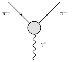
Figure 3.1: The virtual photon-pion vertex

The blob means various virtual processes caused by the strong interactions and theoretically it is expressed by a matrix element $\langle p_{2}|J_{\mu}^{EM}(0)|p_{1}\rangle$ of the electromagnetic current $J_{\mu}^{EM}(x)$ of the pion, that can be decomposed into a sum of products of invariant coefficients and linearly independent covariants constructed now only from the four-momenta $p_{1},p_{2}$ as the spin of the pion is zero.

The corresponding coefficients, so-called invariant FFs, are functions of only one invariant variable.

Really, from the conservation of four-momenta at the virtual photon-pion vertex

$$p_{1}+q=p_{2}$$ (3.3)

and by a multiplication of both sides of the latter by one after the other four-momenta $q$, $p_{1}$ and $p_{2}$, one gets a system of the following three algebraic equations

$$(qp_{1})+q^{2} = (qp_{2})$$

$$p_{1}^{2}+(qp_{1}) = (p_{1}p_{2})$$ (3.4)

$$(p_{1}p_{2})+(qp_{2}) = p_{2}^{2}$$

for four unknown invariant variables, $(qp_{1})$, $(qp_{2})$, $q^{2}$, and $(p_{1}p_{2})$, provided $p_{1}^{2}=p_{2}^{2}=-m_{\pi}^{2}$, where $m_{\pi}$ is the pion mass.

By a solution of (3.4) one can express three invariant variables by means of an arbitrary value of the fourth one. The latter is usually chosen to be just the four-momentum transfer squared $t=q^{2}=-Q^{2}$.

A decomposition of the matrix element of the pion electromagnetic current looks as follows

$$\langle p_{2}|J_{\mu}^{EM}(0)|p_{1}\rangle=e[F_{\pi}^{E}(t)(p_{1}+p_{2})_{\mu}+G_{\pi}^{E}(t)(p_{2}-p_{1})_{\mu}]$$ (3.5)

where instead of two independent four-momenta $p_{1}$, $p_{2}$ we have used their suitable combinations, $(p_{1}+p_{2})_{\mu}$ and $(p_{2}-p_{1})_{\mu}=q_{\mu}$ and $F_{\pi}^{E}(t)$, $G_{\pi}^{E}(t)$ are invariant FFs.

The gauge invariance of the EM interactions implies the current conservation

$$\partial_{\mu}J_{\mu}^{EM}(x)=0$$ (3.6)

from where the following condition

$$q_{\mu}\langle p_{2}|J_{\mu}^{EM}(0)|p_{1}\rangle=0$$ (3.7)

has to be fulfilled. Since $q_{\mu}(p_{1}+p_{2})_{\mu}=p_{2}^{2}-p_{1}^{2}=0$, the condition (3.7) will be valid if in (3.5) $G_{\pi}^{E}(t)=0$. Then the matrix element of the pion EM current takes finally the well-known form

$$\langle p_{2}|J_{\mu}^{EM}(0)|p_{1}\rangle=eF_{\pi}^{E}(t)(p_{1}+p_{2})_{\mu},$$ (3.8)

where $F_{\pi}^{E}(t)$ is the so-called pion EM FF.

On the other hand, making use of transformation properties of the EM current operator $J_{\mu}^{EM}(x)$ and the one-particle state vectors of pions, $|\pi^{+}\rangle$, $|\pi^{-}\rangle$ and $|\pi^{0}\rangle$, with regard to the all three discrete $C$, $P$, $T$ transformations simultaneously, one can derive relations as follows

$$\langle\pi^{-}|J_{\mu}^{EM}(0)|\pi^{-}\rangle=-\langle\pi^{+}|J_{\mu}^{EM}(0)|\pi^{+}\rangle$$ (3.9)

and

$$\langle\pi^{0}|J_{\mu}^{EM}(0)|\pi^{0}\rangle=-\langle\pi^{0}|J_{\mu}^{EM}(0)|\pi^{0}\rangle.$$ (3.10)

Then a substitution of the parametrization (3.8) into (3.9) and (3.10) provides for the EM FFs of charged and neutral pions relations

$$F_{\pi^{-}}^{E}(t)=-F_{\pi^{+}}^{E}(t)$$ (3.11)

and

$$F_{\pi^{0}}^{E}(t)\equiv 0,$$ (3.12)

respectively, for all values of the four-momentum transfer squared $-\infty<t<+\infty$.

Since the charge $e$ appears as a prefactor in (3.8), the pion EM FF at $t=0$ is normalized to one

$$F_{\pi}^{E}(0)=1.$$ (3.13)

In the framework of the axiomatic quantum field theory one can prove [15] that $F_{\pi^{\pm}}(t)$ is an analytic function in the whole complex $t$- plane, besides a cut from $4m_{\pi}^{2}$ to $+\infty$. The same analytic properties can be derived within the framework of QCD [20]. Further, as a consequence of the pion EM current $J_{\mu}^{E}(x)$ to be Hermitian, the pion EM FF is real on the real axis for $t<4m^{2}_{\pi}$. Then by an application of the Schwarz reflection principle to the pion EM FF one finds the so-called reality condition

$$[F_{\pi}^{E}(t)]^{*}=F_{\pi}^{E}(t^{*})$$ (3.14)

reflecting the reality of the pion EM FF on the real axis below $4m^{2}_{\pi}$ and the relation of values of the pion EM FF on the upper and lower boundary of the cut

$$[F_{\pi}^{E}(t+i\epsilon)]^{*}=F_{\pi}^{E}(t-i\epsilon),\quad\quad\quad\quad\quad\quad\quad\quad\epsilon\ll 1$$ (3.15)

automatically.

The discontinuity across the cut is given by the unitarity condition

$$\frac{1}{2i}\left\{\langle\pi^{+}\pi^{-}|J_{\mu}^{EM}(0)|0\rangle-\langle 0|J_{\mu}^{EM}(0)|\pi^{+}\pi^{-}\rangle^{*}\right\}=\sum_{n}\langle\pi^{+}\pi^{-}|T^{+}|n\rangle\langle n|J_{\mu}^{EM}(0)|0\rangle,$$ (3.16)

where

$$\langle\pi^{+}\pi^{-}|J_{\mu}^{EM}(0)|0\rangle=e(k_{\pi^{+}}-k_{\pi^{-}})_{\mu}F_{\pi}^{E}(t)$$ (3.17)

is a matrix element of the pion EM current defining the pion EM FF in the time-like ($t>4m^{2}_{\pi}$) region. The sum in (3.16) is carried out over a complete set of intermediate states allowed by various conservation laws and $T^{+}$ means Hermitian conjugate amplitudes.

Moreover, the unitarity condition (3.16) tells us that there is an infinite number of branch points on the positive real axis between $t=4m^{2}_{\pi}$ and $+\infty$, which always correspond to a new allowed intermediate state $n$ in (3.16). In order to fulfil the reality condition (3.14), the cuts associated with these branch points are chosen to extend to $+\infty$ along the real axis.

We would like to note that one can specify [16, 17, 18] the same singularities of the pion EM FF by means of an investigation of the analytic properties of the corresponding Feynman diagrams of a formal pion EM FF perturbation series.

Consequently, the first branch point of the pion EM FF is at $t=4m^{2}_{\pi}$, the second one at $t=16m^{2}_{\pi}$, then at $t=(m_{\pi^{0}}+m_{\omega})^{2}$, $t=4m_{K}^{2}$, etc.

If we restrict ourselves in (3.16) only to $|n\rangle=|\pi^{+}\pi^{-}\rangle$, then the elastic unitarity condition of the pion EM FF is obtained

$$\frac{1}{2i}\left\{F_{\pi}^{E}(t+i\epsilon)-[F_{\pi}^{E}(t+i\epsilon)]^{*}\right\}=[A^{1}_{1}(t+i\epsilon)]^{*}F_{\pi}^{E}(t+i\epsilon)$$ (3.18)

where $A^{1}_{1}(t+i\epsilon)$ is the $P$- wave isovector $\pi\pi$- scattering amplitude.

If the complete set of intermediate states in (3.16) is taken into account then the pion EM FF unitarity condition can be written in the form

$$\frac{1}{2i}\left\{F_{\pi}^{E}(t+i\epsilon)-[F_{\pi}^{E}(t+i\epsilon)]^{*}\right\}=[A^{1}_{1}(t+i\epsilon)]^{*}F_{\pi}^{E}(t+i\epsilon)+\sigma(t+i\epsilon)$$ (3.19)

where $\sigma(t+i\epsilon)$ represents all higher contributions.

Now we prove that the lowest singularity of the pion EM FF at $t=4m^{2}_{\pi}$ is a square-root type branch point.

The idea consists in the analytic continuation of the pion EM FF through the upper and lower boundary of the cut between $t=4m^{2}_{\pi}$ and $t=16m^{2}_{\pi}$ on the next sheet of the Riemann surface by means of the elastic unitarity condition (3.18) and in a subsequent comparison of obtained functional expressions.

By using the reality condition of the pion EM FF (3.14) and similar condition [21]

$$[A^{1}_{1}(t+i\epsilon)]^{*}=-A^{1}_{1}(t-i\epsilon)$$ (3.20)

for the $P$- wave isovector $\pi\pi$ - scattering amplitude, one can rewrite (3.18) into the form as follows

$$F_{\pi}^{E}(t+i\epsilon)=\frac{F_{\pi}^{E}(t-i\epsilon)}{1+2iA^{1}_{1}(t-i\epsilon)}.$$ (3.21)

If we denote by $[F_{\pi}^{E}(t-i\epsilon)]^{+}$ and $[F_{\pi}^{E}(t+i\epsilon)]^{-}$ the analytic continuation of the pion EM FF on the Riemann sheets achieved through the upper and lower boundary of the elastic cut, respectively, then as a consequence of a continuity of the pion EM FF we have

$$[F_{\pi}^{E}(t-i\epsilon)]^{+}\equiv F_{\pi}^{E}(t+i\epsilon)$$ (3.22)

$$[F_{\pi}^{E}(t+i\epsilon)]^{-}\equiv F_{\pi}^{E}(t-i\epsilon).$$ (3.23)

Then by a substitution of (3.22) into (3.21) one gets

$$[F_{\pi}^{E}(t-i\epsilon)]^{+}=\frac{F_{\pi}(t-i\epsilon)}{1+2iA^{1}_{1}(t-i\epsilon)}.$$ (3.24)

On the other hand, by a complex conjugation of (3.18) and the reality conditions (3.15) and (3.20), the unitarity condition of the pion EM FF on the lower boundary of the elastic cut is obtained

$$\frac{1}{2i}\left\{F_{\pi}^{E}(t-i\epsilon)-[F_{\pi}^{E}(t-i\epsilon)]^{*}\right\}=\{A^{1}_{1}(t-i\epsilon)\}^{*}F_{\pi}^{E}(t-i\epsilon),$$

from which the relation follows

$$F_{\pi}^{E}(t-i\epsilon)\{1+2iA^{1}_{1}(t+i\epsilon)\}=F_{\pi}^{E}(t+i\epsilon)$$

or by using (3.23), finally one gets

$$[F_{\pi}^{E}(t+i\epsilon)]^{-}=\frac{F_{\pi}^{E}(t+i\epsilon)}{1+2iA^{1}_{1}(t+i\epsilon)}.$$ (3.25)

Comparing (3.25) with (3.24) we see that by the analytic continuation of the pion EM FF through upper and lower boundary of the elastic cut one gets the identical functional expressions. The latter convinces us that one has come on the same sheet of the Riemann surface, which further will be called the second one and denoted by II. It follows just from here that the branch point $t=4m^{2}_{\pi}$ is of a square-root type, i.e. it generates just two sheets of the Riemann surface, on which the pion EM FF is defined.

Moreover, the analytic continuation of (3.24) and (3.25) leads to the same expression of the pion EM FF on the second Riemann sheet as follows

$$[F_{\pi}^{E}(t)]^{II}=\frac{F_{\pi}^{E}(t)}{1+2iA^{1}_{1}(t)}.$$ (3.26)

One can read out from (3.26), that the pion EM FF on the second Riemann sheet has all the branch points of the pion EM FF on the first sheet and besides also the branch points of the $P$- wave isovector $\pi\pi$- scattering partial amplitude $A^{1}_{1}(t)$.

It is well known [21] that the analytic properties of $A^{1}_{1}(t)$ consist of the right-hand unitary cut for $4m^{2}_{\pi}<t<\infty$ and the left-hand dynamical cut for $-\infty<t<0$. From the latter and (3.26) it follows that the pion EM FF on the second Riemann sheet has the left hand cut too.

The unitarity condition in the language of the $S^{1}_{1}(t)$ matrix, connected with the amplitude $A^{1}_{1}(t)$ in (3.26) by the relation

$$S^{1}_{1}(t)=1+2iA^{1}_{1}(t),$$ (3.27)

has the form

$$S^{1}_{1}(t)[S^{1}_{1}(t)]^{*}=1$$ (3.28)

from where one can parametrize

$$S^{1}_{1}(t)=e^{2i\delta_{1}^{1}(t)}$$ (3.29)

with $\delta_{1}^{1}(t)$ to be the $P$- wave isovector $\pi\pi$-scattering phase shift. By means of a substitution of (3.27) into (3.28) one gets the unitarity condition for $A^{1}_{1}(t)$ in the form

$$ImA^{1}_{1}(t)=|A^{1}_{1}(t)|^{2}$$ (3.30)

which is exactly valid for $4m_{\pi}^{2}<t<16m_{\pi}^{2}$. However it follows just from data [22, 23, 24] on $A^{1}_{1}(t)$ that it works approximately up to 1${\rm GeV}^{2}$.

On the other hand by a combination of the relations (3.29) and (3.27), the following parametrization of $A^{1}_{1}(t)$ is obtained

$$A_{1}^{1}(t)=\frac{1}{2i}\left(e^{2i\delta^{1}_{1}(t)}-1\right)=e^{i\delta^{1}_{1}(t)}\sin\delta_{1}^{1}(t)$$ (3.31)

which is consistent with the unitarity condition (3.30) automatically.

We note, that the partial wave amplitude $A^{1}_{1}(t)$ has a resonant behavior as the derivative $d\delta^{1}_{1}(t)/dt$ has a pronounced maximum to be not caused by an opening of some new threshold. Since $A^{1}_{1}(t)$ is an analytic function, the rapid variation of $\delta^{1}_{1}(t)$ can be described by a pole in the second Riemann sheet, which corresponds just to the well known $\rho$(770) resonance. Farther, starting only from general considerations we show that the latter pole has to appear also on the second Riemann sheet of the pion EM FF.

Really, starting from the unitarity condition (3.30), analogically to the pion EM FF, one can prove that the branch point $4m_{\pi}^{2}$ of the amplitude $A_{1}^{1}(t)$ is a square root type and also one can find an expression of the amplitude $A^{1}_{1}$ on the second Riemann sheet to be

$$[A_{1}^{1}(t)]^{II}=-\frac{A^{1}_{1}(t)}{1+2iA^{1}_{1}(t)}.$$ (3.32)

By a comparison of (3.32) and (3.26) we see they have an identical denominator. So, if $[A_{1}^{1}(t)]^{II}$ has the $\rho$(770)-meson pole created by a zero of the denominator $1+2iA^{1}_{1}(t)$, then the same zero has to be present in the denominator of $[F_{\pi}(t)]^{II}$, and as a consequence, the $\rho$(770)- meson pole has to be created on the second Riemann sheet of the pion EM FF.

Since such a pole is shifted (due to the instability of $\rho$(770)) from the real axis into the complex plane, as a result of the reality condition (3.14), there must exist also the complex conjugate pole to the latter.

We note, there are radial excitations [12] of the $\rho$(770)-meson. The corresponding poles are also placed on the unphysical sheets of the Riemann surface on which the pion EM FF is defined. Then all information on the analytic properties of the pion EM FF looks like it is presented in Fig. 3.2.

Figure 3.2: Analytic properties of the pion EM FF

Defining a phase of the pion EM FF for $t>4m_{\pi}^{2}$ by the relation

$$F_{\pi}^{E}(t)=|F_{\pi}^{E}(t)|e^{i\delta_{\pi}(t)}$$ (3.33)

and substituting the latter, together with (3.31), into the unitarity condition (3.18) one finds the identity

$$\delta_{\pi}(t)\equiv\delta_{1}^{1}(t)$$ (3.34)

valid in the whole elastic region.

The next property of the pion EM FF follows from the threshold behavior of the $P$-wave isovector $\pi\pi$- scattering partial wave amplitude

$$A^{1}_{1}(t)_{|_{q\to 0}}\sim a^{1}_{1}q^{3}$$ (3.35)

where $a^{1}_{1}$ is the $P$- wave isovector $\pi\pi$- scattering length and $q$ is the absolute value of the pion three momentum in the center of mass (c.m.) system, which is connected with the momentum transfer squared by the following relation

$$t=4(q^{2}+m_{\pi}^{2}).$$ (3.36)

Taking into account (3.35) and the parametrization (3.31) for $q\to 0$ one gets the threshold behavior of the phase $\delta_{1}^{1}(t)_{q\to 0}\sim a_{1}^{1}q^{3}$ which by means of the (3.34) gives the threshold behavior of the pion EM FF phase

$$\delta_{\pi}(t)_{|_{q\to 0}}\sim a_{1}^{1}q^{3}.$$ (3.37)

One of the basic properties of the EM FFs of strongly interacting particles is their asymptotic behavior. However, until the discovery of the quark-gluon structure of hadrons the latter was unknown theoretically and only polynomial bounds were always assumed to be fulfilled.

According to the quark model, the large momentum transfer behavior of the hadron EM FF is related to the number of constituent quarks of the considered hadron (2.24). Thus for the pion $(n_{q}=2)$ one gets (3.1), which is in a qualitative agreement with existing data. This is a prediction of a dimensional counting rule and some simple assumptions which are based on the case of an underlying scale-invariant theory [3, 4].

The asymptotic behavior (3.1) of the pion EM FF was proved [5, 6, 7] (up to the logarithmic correction) in the framework of the perturbative QCD. Here the pion EM FF takes the following form [5] (see Fig. 3.3)

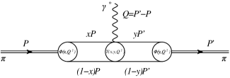
Figure 3.3: Representation of the pion FF in QCD.

$$F_{\pi}^{E}(Q^{2})=\int_{0}^{1}dx\int_{0}^{1}dy\Phi^{+}(y,Q^{2})T(x,y,Q^{2})\Phi(x,Q^{2})$$ (3.38)

where $\Phi(x,Q^{2})$ is a wave function of the pion, which represents a probability to find the quark to carry the fractional momentum $x$ of the total pion momentum and $T(x,y,Q^{2})$ is the amplitude of an interaction of the virtual photon with quarks and gluons. For the latter one can write the following perturbative expansion

$$T(x,y,Q^{2})=\alpha_{s}(Q^{2})T_{B}(x,y,Q^{2})\left[1+\alpha_{s}(Q^{2})T_{2}(x,y,Q^{2})+....\right]$$ (3.39)

where $\alpha_{s}(Q^{2})$ is the effective constant of the quark-gluon interactions defined (in the lowest order) by the expression

$$\alpha_{s}(Q^{2})=\frac{4\pi}{(11-2/3n_{f})\ln{Q^{2}/\Lambda^{2}}}$$ (3.40)

with $n_{f}$ to be a quark number flavor and $\Lambda$ as a QCD scale parameter.

In the lowest order according to $\alpha_{s}(Q^{2})$ there are contributing only two Feynman diagrams (see Fig. 3.4) into $T(x,y,Q^{2})$.

Figure 3.4: Dominating Feynman diagrams in the lowest order according to $\alpha_{s}(Q^{2})$.

By means of a calculation of the latter one gets an explicit form for the Born approximation $T_{B}$ of the amplitude $T(x,y,Q^{2})$ to be

$$T_{B}(x,y,Q^{2})=\frac{16\pi C_{F}}{Q^{2}(1-x)(1-y)}$$

where $C_{F}=3/4$ is the so-called colour factor.

Now one has to find $\Phi(x,Q^{2})$. It satisfies the differential equation (see e.g.[25, 26])

$$\frac{d\Phi(x,Q^{2})}{d\kappa}=\int_{0}^{1}duV_{q\bar{q}\to q\bar{q}}(u,x)\Phi(u,Q^{2})$$ (3.41)

in which

$$\kappa=2/\beta_{0}\ln{\frac{\alpha_{s}(Q^{2}_{0})}{\alpha_{s}(Q^{2})}},\quad\quad\quad\quad\quad\beta=11-2/3n_{f}$$

and the kernel takes the form [5] as follows

$$V_{q\bar{q}\to q\bar{q}}(u,x)=1/2C_{F}\left\{\frac{1-u}{1-x}(1+\frac{1}{u-x})_{+}\Theta(u-x)+\frac{u}{x}(1+\frac{1}{x-u})_{+}\Theta(x-u)\right\}.$$ (3.42)

If the function $\Phi(x,Q^{2})$ is known at $Q^{2}_{0}$, then by using the equation (3.41) one can calculate it for arbitrary value $Q^{2}$. In principle $Q^{2}_{0}$ can be chosen to be arbitrary as soon as the condition

$$\frac{\alpha_{s}(Q^{2}_{0})}{4\pi}<1$$ (3.43)

is fulfilled.

The equation (3.41) can be solved easily if the property [5]

$$\int_{0}^{1}dzC_{n}^{(3/2)}(2z-1)V_{q\bar{q}\to q\bar{q}}(z,x)=1/2A_{n}^{NS}C_{n}^{3/2}(x)$$ (3.44)

is used, where

$$A_{n}^{NS}=C_{F}\left[-\frac{1}{2}+\frac{1}{(n+1)(n+2)}-2\sum_{j=2}^{n+1}\frac{1}{j}\right]$$ (3.45)

are the so-called non-singlet anomalous dimensions and $C_{n}^{3/2}(x)$ are the Gegenbauer polynomials of the order 3/2.

If one decomposes $\Phi(x,Q^{2})$ into a series according to the polynomials $C_{n}^{(3/2)}(x)$ as follows

$$\Phi(x,Q^{2})=x(1-x)\sum_{n=0}^{\infty}\Phi_{n}(Q^{2})C_{n}^{(3/2)}(2x-1)$$ (3.46)

and then substitute it into (3.41), one gets the equation for the coefficients of the previous expansion in the form

$$\frac{d\Phi_{n}(Q^{2})}{d\kappa}=A_{n}^{NS}\Phi_{n}(Q^{2}).$$ (3.47)

By means of a solution of the latter one obtains

$$\Phi_{n}(Q^{2})=exp(\kappa A^{NS}_{n})\Phi_{n}(Q^{2}_{0})\equiv\left\{\frac{\alpha_{s}(Q^{2})}{\alpha_{s}(Q_{0}^{2})}\right\}^{d_{n}}\Phi_{n}(Q_{0}^{2})$$ (3.48)

where

$$d_{n}=-2A_{n}^{NS}/\beta_{0}.$$ (3.49)

Now collecting all partial results we come to the expression of the pion EM FF

$$F_{\pi}^{E}(Q^{2})=4\pi(\frac{4}{3})\frac{\alpha_{s}(Q^{2})}{Q^{2}}\left|\sum_{n=0}^{\infty}\Phi_{n}(Q^{2}_{0})\left\{\frac{\alpha_{s}(Q^{2})}{\alpha_{s}(Q_{0}^{2})}\right\}^{d_{n}}\right|$$ (3.50)

from which the relation

$$F_{\pi}^{E}(Q^{2})=4\pi(\frac{4}{3})\frac{\alpha_{s}(Q^{2})}{Q^{2}}\left[|\Phi_{0}(Q^{2}_{0})|^{2}+2Re\quad(\Phi_{0}(Q^{2}_{0})\Phi^{*}_{1}(Q^{2}_{0}))\left\{\frac{\alpha_{s}(Q^{2})}{\alpha_{s}(Q^{2}_{0})}\right\}^{d_{1}}+...\right]$$ (3.51)

follows with $d_{1}$=0.427 for $n_{f}$=4.

If one restricts in the previous result only to the first leading term, then

$$F_{\pi}^{E}(Q^{2})=4\pi(\frac{4}{3})\frac{\alpha_{s}(Q^{2})}{Q^{2}}|\Phi_{0}(Q_{0}^{2})|^{2}.$$

In this case Farrar and Jackson have found [6] the relation

$$\Phi_{0}(Q_{0}^{2})={\sqrt{3}}f_{\pi},$$ (3.52)

where $f_{\pi}=92.4\pm 0.2\,{\rm MeV}$ is the constant of the weak pion decay into $\mu$- meson and antineutrino. As a result one comes to the expression for the asymptotic behavior of the pion EM FF

$$F_{\pi}^{E}(Q^{2})_{Q^{2}\to\infty}\sim\frac{16\pi f_{\pi}^{2}\alpha_{s}(Q^{2})}{Q^{2}}$$ (3.53)

or by using (3.40)

$$F_{\pi}^{E}(Q^{2})_{Q^{2}\to\infty}\sim\frac{64\pi^{2}f_{\pi}^{2}}{(11-2/3n_{f})Q^{2}\ln{Q^{2}/\Lambda}}$$ (3.54)

which confirms (up to the logarithmic correction) the quark counting rule prediction (3.1).

Higher orders in (3.51) depend on the models chosen for the pion wave function.

Till now we have considered only the invariant pion EM FF in the momentum representation to be sufficient for a description of observable phenomena.

Nevertheless, there is a special Breit system in which the space-component of the pion EM current is equal to zero and as a consequence one can write down there the Fourier transform of the pion EM FF giving just the static charge distribution density as follows

$$\rho(\vec{r})=\frac{1}{(2\pi)^{3}}\int F_{\pi}^{E}(\vec{Q}^{2})e^{i\vec{Q}\vec{r}}d^{3}Q.$$ (3.55)

The inverse Fourier transform to (3.55) has the following form

$$F_{\pi}^{E}(\vec{Q}^{2})=\int\rho(\vec{r})e^{-i\vec{Q}\vec{r}}d^{3}r.$$ (3.56)

If $\rho(\vec{r})$ is a spherically symmetric distribution, then one can rewrite (3.56) into the spherical coordinates and by an integration over $\theta$ and $\varphi$ angles one gets

$$F_{\pi}^{E}(\vec{Q}^{2})=4\pi\int_{0}^{\infty}\frac{\sin Qr}{Qr}\rho(\vec{r})r^{2}dr.$$

For the case of $Qr\ll 1$

$$\sin Qr\simeq Qr-\frac{(Qr)^{3}}{6}+......$$

and

$$F_{\pi}^{E}(\vec{Q}^{2})=4\pi\int_{0}^{\infty}r^{2}\rho(\vec{r})dr-\frac{4\pi Q^{2}}{6}\int_{0}^{\infty}r^{4}\rho(\vec{r})dr+...\cdot$$

Now, taking into account the charge distribution density normalization

$$\int_{0}^{\infty}\rho(\vec{r})4\pi r^{2}dr=1$$

and a definition of the mean square charge radius

$$\langle r^{2}_{\pi}\rangle=\int_{0}^{\infty}r^{2}\rho(\vec{r})4\pi r^{2}dr$$

one gets finally

$$F_{\pi}^{E}(\vec{Q}^{2})=1-\frac{Q^{2}}{6}\langle r^{2}_{\pi}\rangle+...$$

from where the well known rule for a calculation of the mean square pion charge radius

$$\langle r^{2}_{\pi}\rangle=6\frac{dF_{\pi}^{E}(t)}{dt}_{|_{t=0}}$$ (3.57)

is obtained.

From the relations (3.11), (3.12) and (3.57) it is transparent to see that the mean square charge radius of the $\pi^{+}$- meson takes a positive value, the mean square charge radius of the $\pi^{-}$- meson takes a negative value and the mean square charge radius of the $\pi^{0}$- meson is identically to be zero.

3.2 Experimental information on the absolute value of charged pions form factor

The pion EM FF is the simplest one of all others EM FFs of hadrons, the absolute value of which can be measured (directly or indirectly) everywhere on the real axis of the complex $t$-plane, on which the pion EM FF is defined, by using the following five different processes

• the electroproduction of pions on nucleons ($e^{-}N\to e^{-}\pi N$);

• the scattering of charged pions on atomic electrons; ($\pi^{-}e^{-}\to\pi^{-}e^{-}$)

• the inverse electroproduction processes ($\pi^{-}p\to e^{+}e^{-}n$);

• the electron-positron annihilation into two charged pions; ($e^{+}e^{-}\to\pi^{+}\pi^{-}$)

• $J/\Psi$ decay into two charged pions ($J/\Psi\to\pi^{+}\pi^{-}$).

Up to the present time there are more than 25 independent experiments realized in which an information on $|F^{E}_{\pi}(t)|$ in the space-like ($t<0$) and in the time-like ($t>0$) regions, for the range of momenta $-10{\rm GeV}^{2}<t<10{\rm GeV}^{2}$, was obtained.

The crucial (though not very precise) experiment was carried out in Novosibirsk [27], where the cross-section on the $e^{+}e^{-}\to\pi^{+}\pi^{-}$ process was measured and an information on $|F^{E}_{\pi}(t)|$ at the region of the $\rho$(770)- resonance was extracted. As a result, a creation of the $\rho(770)$- meson in the electron-positron annihilation into hadrons was confirmed experimentally for the first time. Later on this resonant region was re-measured with a higher precision in ORSAY [28] and the isospin violating $\omega(782)\to\pi^{+}\pi^{-}$ decay contribution to $e^{+}e^{-}\to\pi^{+}\pi^{-}$ process, the so-called $\rho-\omega$ interference effect, was experimentally revealed.

Afterwards, during the next four decades many new experiments with the aim of obtaining of the experimental information on the pion EM FF in the space-like and time-like regions were proposed and realized.

Since the pion is an unstable particle, one can not make a fixed pion target experiment of the elastic electron scattering on pions, like on the protons, in order to investigate the pion EM structure in the space-like region. Therefore, for very small values of $t$, the scattering of charged pions on atomic electrons, $\pi^{-}e^{-}\to\pi^{-}e^{-}$, was employed [29, 30] and for higher negative values of $t$ the electro-production process, $e^{-}N\to e^{-}\pi N$, was used [31, 32, 33].

In the time-like region, for $0<t<4m^{2}_{\pi}$, an information on $|F_{\pi}^{E}(t)|$ was obtained [34, 35, 36] from data on the inverse electro-production process $\pi^{-}p\to e^{-}e^{+}n$. Also the process $\bar{p}n\to\pi^{-}\ell^{+}\ell^{-}$ is a suitable candidate [37] for the latter, provided that all corresponding nucleon EM FFs are known in this region.

On the other hand, as the process $e^{+}e^{-}\to\pi^{+}\pi^{-}$ is of the EM nature, one can treat the latter in the one-photon-exchange approximation and as a result, there are no model ingredients in an extraction of $|F_{\pi}^{E}(t)|$ from the measured cross-section of the process under consideration. Therefore, the most reliable up to now information on the $|F_{\pi}^{E}(t)|$ was obtained in a systematic investigations of the $e^{+}e^{-}\to\pi^{+}\pi^{-}$ process in ORSAY [38, 39, 40], Frascati [41, 42, 43], Novosibirsk [44, 45, 46] and CERN [47].

Figure 3.5: Experimental data on $|F_{\pi}^{E}(t)|$

The experimental point on $|F_{\pi}^{E}(t)|$ at the highest value of $t$, $t$= 9.579 ${\rm GeV}^{2}$, was obtained [48] from the $J/\Psi\to\pi^{+}\pi^{-}$ decay, which must be electromagnetic (i.e. it is realized through one virtual photon) provided that the $G$- parity is conserved by strong interactions.

As a result there are more than 300 experimental points on $|F_{\pi}^{E}(t)|$ (see Fig. 3.5) for the range of momenta $-10{\rm GeV}^{2}<t<+10{\rm GeV}^{2}$. However, they do not seem to be all mutually consistent and as a result too high values of the $\chi^{2}/{\rm NDF}$ is in the fitting procedure by $U\&A$ pion EM FF models found.

3.3 Unitary and analytic model of charged pions electromagnetic structure

Further we present a construction of the model which reflects all known properties of $F_{\pi}^{E}(t)$, including also the threshold behavior of $ImF_{\pi}^{E}(t)$ and describes all existing data. It represents just the most accomplished pion electromagnetic structure model to be constructed up to now.

However, first very briefly all known properties of the pion EM FF are reviewed.

• The function $F_{\pi}^{E}(t)$ is normalized (3.13) at $t=0$.

• $F_{\pi}^{E}(t)$ can be considered as a complex function of a complex variable $t$ and it is analytic function in the whole complex $t$-plane besides the cut from $4m^{2}_{\pi}$ to $+\infty$.

• A discontinuity across the latter cut is given by the unitarity condition (3.16), in which the first three allowed intermediate states are $|\pi^{+}\pi^{-}\rangle$ $|\pi^{+}\pi^{-}\pi^{+}\pi^{-}\rangle$ and $|\pi^{0}\omega\rangle$.

• To every intermediate state $|n\rangle$ in the unitarity condition (3.16) a branch point corresponds at the value of $t$ to be equal to the squared sum of masses of the corresponding particles, i.e. they are at $t=(2m_{\pi})^{2}$ , $(4m_{\pi})^{2}$, $(m_{\pi^{0}}+m_{\omega})^{2}$, etc..

• From the Hermitivity of $J_{\mu}^{EM}$ i.e.

  $$(J_{\mu}^{EM})^{+}=J_{\mu}^{EM}$$ (3.58)

  the reality of $F_{\pi}^{E}(t)$ on the real axis from $-\infty$ to $4m_{\pi}^{2}$ and the reality condition (3.14), as well as a relation (3.15) between values of $F_{\pi}^{E}(t)$ on the upper $(t+i\epsilon)$ and lower $(t-i\epsilon)$ boundary of the cut ( $t>4m^{2}_{\pi}$) follow.

• By using of (3.18) one can continue analytically $F_{\pi}^{E}(t)$ through the upper and lower boundary of the cut at the interval $4m^{2}_{\pi}<t<16m^{2}_{\pi}$ and simultaneously one can prove in a such way that the first branch point at $t=4m_{\pi}^{2}$ is a square root type.

• As a by-product of the latter one obtains the expression (3.26) for the pion EM FF on the second sheet of the Riemann surface on which $F_{\pi}^{E}(t)$ is completely defined as an unambiguous function of $t$.

• One can read out from (3.26) the analytic properties of $F_{\pi}^{E}(t)$ on the second Riemann sheet. As the analytic properties of $A^{1}_{1}$ on the first (physical) Riemann sheet consist of the right-hand unitary cut for $4m_{\pi}^{2}<t<+\infty$ and the left hand dynamical cut for $-\infty<t<0$, the pion EM FF on the second Riemann sheet has the left hand cut for $-\infty<t<0$ too. In order to obtain a correct reproduction of the pion EM FF phase, a contribution of the latter can not be neglected as it was done in many phenomenological models in the past.

• As the $\pi\pi$ scattering amplitude is dominated by the $\rho$(770) resonance to be placed in the form of the pole on the second sheet and $[A^{1}_{1}]^{II}(t)$ has identical denominator with (3.26), then $F_{\pi}^{E}(t)$ has also the pole on the second Riemann sheet corresponding just to the $\rho$(770) resonance. All excited states of $\rho$(770) are also placed on some unphysical sheets of the constructed Riemann surface.

• As a consequence of the reality condition (3.14) to every resonance pole also a complex conjugate pole has to exist .

• The identity (3.34) is practically valid for $4m_{\pi}^{2}<t\leq 1{\rm{\rm GeV}}^{2}$.

• Directly from (3.33) the imaginary part of the pion EM FF takes the form

  $$ImF_{\pi}^{E}(t)=|F_{\pi}^{E}(t)|\sin\delta_{\pi}(t)$$ (3.59)

  from where by using (3.37) one gets the threshold behavior of the pion EM FF imaginary part

  $$ImF_{\pi}^{E}(t)_{|_{q=0}}=|F_{\pi}^{E}(t)|a^{1}_{1}q^{3}$$ (3.60)

  which can be transformed into the following three conditions

  $$ImF_{\pi}^{E}(t)_{|_{q=0}}=\frac{dImF_{\pi}^{E}(t)}{dq}_{|_{q=0}}=\frac{d^{2}ImF_{\pi}^{E}(t)}{dq^{2}}_{|_{q=0}}=0.$$ (3.61)

• The $\pi\pi$ scattering length $a^{1}_{1}$ in (3.35) can be calculated from the pion EM FF by means of the expression

  $$a^{1}_{1}=\frac{\frac{d^{3}ImF_{\pi}^{E}(t)}{dq^{3}}}{6|F_{\pi}^{E}(t)|}_{|_{q=0}}.$$ (3.62)

• The asymptotic behavior (3.54) of the pion EM FF obtained in the framework of the pQCD is equivalent (up to the logarithmic correction) to the quark counting rule prediction (3.1).

To our knowledge there are no other properties of $F_{\pi}^{E}(t)$ to be known for the time being.

Starting from the general parametrization (3) one obtains for the pion EM FF the expression

$$F_{\pi}^{E}[W(t)] = \left(\frac{1-W^{2}}{1-W_{N}^{2}}\right)^{2}\times$$

$$\times \left[\frac{(W_{N}-W_{\rho})(W_{N}-W_{\rho}^{*})(W_{N}-1/W_{\rho})(W_{N}-1/W_{\rho}^{*})}{(W-W_{\rho})(W-W_{\rho}^{*})(W-1/W_{\rho})(W-1/W_{\rho}^{*})}(\frac{f_{{\rho}\pi\pi}}{f_{\rho}})\right.+$$

$$+ \left.\sum_{v=\rho^{\prime},\rho^{\prime\prime}}\frac{(W_{N}-W_{v})(W_{N}-W_{v}^{*})(W_{N}+W_{v})(W_{N}+W_{v}^{*})}{(W-W_{v})(W-W_{v}^{*})(W+W_{v})(W+W_{v}^{*})}(\frac{f_{v\pi\pi}}{f_{v}})\right]$$

to be defined on the four-sheeted Riemann surface reflecting all above mentioned properties, besides the left-hand cut contribution and the threshold behavior (3.60) of the $ImF_{\pi}^{E}(t)$.

The left hand cut contribution manifests itself mainly about the first $4m^{2}_{\pi}$ threshold as it provides a possibility to achieve a correct ratio of $ImF_{\pi}^{E}(t)$ to $ReF_{\pi}^{E}(t)$ at the expression

$$\tan\delta_{\pi}(t)=\frac{ImF_{\pi}^{E}(t)}{ReF_{\pi}^{E}(t)}$$ (3.64)

and in a such way as a result of (3.34) also a reproduction of the experimental data on $\delta^{1}_{1}(t)$.

From literature it is well known, that the contribution of a cut of an arbitrary analytic function can be in the framework of the Padè approximations represented by alternating zeros and poles on the place of that cut.

This method was employed in [49, 50] to demonstrate explicitly that experimental data on $|F_{\pi}^{E}(t)|$ and $\delta^{1}_{1}(t)$ can be described consistently only by the pion EM FF model including the correct left-hand cut contribution.

Really, in [49] $\tan\delta_{1}^{1}(t)$ was approximated by a rational function in $q$- variable with a minimal number of coefficients to be determined from a fit of data on $\delta^{1}_{1}(t)$. Then by means of a dispersion integral a rational function for $F_{\pi}^{E}(t)$ was obtained in which one zero and one pole just on the place of the cut from the second Riemann sheet were found. The latter result clearly demonstrates that the left-hand cut contribution can not be neglected in any analytic pion EM FF model.

The same result was confirmed in [50] by a different way. Here, first, contributions of the isospin violating $\omega({\rm 783})\to\pi^{+}\pi^{-}$ decay from the data on $\sigma_{tot}(e^{+}e^{-}\to\pi^{+}\pi^{-})$ were separated. Then the resultant data were combined with data on $\delta^{1}_{1}(t)$ in order to get the data on $ReF_{\pi}^{E}(t)$ and $ImF_{\pi}^{E}(t)$. The latter were described by various Padè-type approximants in $q$-variable, in which repeatedly one zero and one pole were identified on the place of the left-hand cut from the second Riemann sheet. Moreover, the found positions are almost identical with those from [49].

By means of the conformal mapping (2.145) the left-hand cut from the second Riemann sheet is mapped into the interval $0<W<+1$. So, on the base of the results obtained in [49, 50] the left-hand cut contribution is in our model approximated by one normalized zero and one normalized pole as follows

$$\frac{(W-W_{z})(W_{N}-W_{p})}{(W_{N}-W_{z})(W-W_{p})}$$ (3.65)

where $W_{z}$ and $W_{p}$ are left to be free parameters.

The most natural incorporation of (3.65) into our model of $F_{\pi}^{E}(t)$ could be as a multiplicative factor to the $\rho$(770)-meson term in (3.3) as the left-hand cut from the second Riemann sheet is near-by to the elastic region $4m^{2}_{\pi}<t<1{\rm GeV}^{2}$.

However, just for the sake of a consistent incorporation of the threshold behavior of $ImF_{\pi}^{E}(t)$, given by (3.60), we incorporate (3.65) as a common factor to all $\rho$-meson resonances contributing to $F_{\pi}^{E}(t)$ as follows

$$F_{\pi}^{E}[W(t)] = \left(\frac{1-W^{2}}{1-W_{N}^{2}}\right)^{2}\frac{(W-W_{z})(W_{N}-W_{p})}{(W_{N}-W_{z})(W-W_{p})}\times$$

$$\times \left\{\frac{(W_{N}-W_{\rho})(W_{N}-W_{\rho}^{*})(W_{N}-1/W_{\rho})(W_{N}-1/W_{\rho}^{*})}{(W-W_{\rho})(W-W_{\rho}^{*})(W-1/W_{\rho})(W-1/W_{\rho}^{*})}(\frac{f_{{\rho}\pi\pi}}{f_{\rho}})\right.+$$

$$+ \left.\sum_{v=\rho^{\prime},\rho^{\prime\prime}}\frac{(W_{N}-W_{v})(W_{N}-W_{v}^{*})(W_{N}+W_{v})(W_{N}+W_{v}^{*})}{(W-W_{v})(W-W_{v}^{*})(W+W_{v})(W+W_{v}^{*})}(\frac{f_{v\pi\pi}}{f_{v}})\right\}.$$

Then all three terms in the wave-brackets give a nonzero contribution to the $ImF_{\pi}^{E}(t)$, though $\rho^{\prime}$- and $\rho^{\prime\prime}$-term (unlike the $\rho$-meson term) are pure real in the interval $4m^{2}_{\pi}<t<t_{in}$. Thus the left hand cut contribution in a consideration of the threshold behavior of $ImF_{\pi}^{E}(t)$ in the $U\&A$ pion EM FF model is crucial.

Now, calculating the $ImF_{\pi}^{E}(t)$ from (3.3) explicitly, one can immediately verify that $ImF_{\pi}^{E}(t)_{|_{q=0}}$=$0$. A requirement of the first derivative of $ImF_{\pi}^{E}(t)$ at $q=0$ to be zero gives the following condition on the coupling constant ratios

$$[(W_{z}-W_{p})+2W_{z}\cdot W_{p}ReW_{\rho}(1+|W_{\rho}|^{-2})]N_{\rho}(f_{\rho\pi\pi}/f_{\rho})+$$

$$+ \sum_{v=\rho^{\prime},\rho^{\prime\prime}}\frac{W_{z}-W_{p}}{|W_{v}|^{4}}N_{v}(f_{v\pi\pi}/f_{v})=0,$$

where

$$N_{\rho}=(W_{N}-W_{\rho})(W_{N}-W_{\rho}^{*})(W_{N}-1/W_{\rho})(W_{N}-1/W_{\rho}^{*})$$

and

$$N_{v}=(W_{N}-W_{v})(W_{N}-W_{v}^{*})(W_{N}+W_{v})(W_{N}+W_{v}^{*}).$$

If condition (3.3) is fulfilled, then the second derivative of $ImF_{\pi}^{E}(t)$ at $q=0$ is automatically zero. The condition (3.3), together with the relation

$$\sum_{v=\rho,\rho^{\prime},\rho^{\prime\prime}}(f_{v\pi\pi}/f_{v})=1,$$ (3.68)

following from the normalization (3.13) and (3.3), give a system of two algebraic equations with three unknown coupling constant ratios. A solution of the latter can be written, e.g. in the form as follows

$$(f_{\rho^{\prime}\pi\pi}/f_{\rho^{\prime}}) = \frac{\frac{N_{\rho^{\prime\prime}}}{|W_{\rho^{\prime\prime}}|^{4}}}{\frac{N_{\rho^{\prime}}}{|W_{\rho^{\prime}}|^{4}}-\frac{N_{\rho^{\prime\prime}}}{|W_{\rho^{\prime\prime}}|^{4}}}-$$

$$- \frac{\frac{N_{\rho^{\prime\prime}}}{|W_{\rho^{\prime\prime}}|^{4}}+\left(1+2\frac{W_{z}.W_{p}}{W_{z}-W_{p}}.Re\left[W_{\rho}(1+|W_{\rho}|^{-2})\right]\right)N_{\rho}}{\frac{N_{\rho^{\prime}}}{|W_{\rho^{\prime}}|^{4}}-\frac{N_{\rho^{\prime\prime}}}{|W_{\rho^{\prime\prime}}|^{4}}}\cdot(f_{\rho\pi\pi}/f_{\rho})$$

$$(f_{\rho^{\prime\prime}\pi\pi}/f_{\rho^{\prime\prime}}) = 1-\frac{\frac{N_{\rho^{\prime\prime}}}{|W_{\rho^{\prime\prime}}|^{4}}}{\frac{N_{\rho^{\prime}}}{|W_{\rho^{\prime}}|^{4}}-\frac{N_{\rho^{\prime\prime}}}{|W_{\rho^{\prime\prime}}|^{4}}}+$$

$$+ \left[\frac{\frac{N_{\rho^{\prime\prime}}}{|W_{\rho^{\prime\prime}}|^{4}}(1+2\frac{W_{z}W_{p}}{W_{z}-W_{p}}.Re[W_{\rho}(1+|W_{\rho}|^{-2})])N_{\rho}}{\frac{N_{\rho^{\prime}}}{|W_{\rho^{\prime}}|^{4}}-\frac{N_{\rho^{\prime\prime}}}{|W_{\rho^{\prime\prime}}|^{4}}}-1\right].(f_{\rho\pi\pi}/f_{\rho})$$

Then the expression (3.3), together with relations (3.3) and (3.3), represents the most accomplished $U\&A$ pion EM FF model, which is defined on four sheeted Riemann surface with complex conjugate poles (corresponding to unstable $\rho$-meson resonances) on unphysical sheets and reflecting all properties (including also the threshold behavior (3.60) of the $ImF_{\pi}^{E}(t)$) briefly reviewed at the beginning of this paragraph. It depends on 10 physically interpretable free parameters, $t_{in}$, $m_{\rho}$, $\Gamma_{\rho}$, $(f_{\rho,\pi\pi}/f_{\rho})$, $m_{\rho^{\prime}}$, $\Gamma_{\rho^{\prime}}$, $m_{\rho^{\prime\prime}}$, $\Gamma_{\rho^{\prime\prime}}$, $W_{z}$ and $W_{p}$. They are determined from the fit of existing reliable experimental points on $|F_{\pi}^{E}(t)|$, containing, however, also a contribution of the isospin violating $\omega({\rm 783})\to\pi^{+}\pi^{-}$ decay, leading to the so-called $\rho-\omega$ interference effect, which can not be excluded by experimentalists in a measurement of $\sigma_{tot}(e^{+}e^{-}\to\pi^{+}\pi^{-})$. In order to take into account the latter effect we have carried out the fit of data by

$$|F_{\pi}^{E}[W(t)]+Re^{i\phi}\frac{m^{2}_{\omega}}{m^{2}_{\omega}-t-im_{\omega}\Gamma_{\omega}}|$$ (3.71)

where

$$\phi=\arctan{\frac{m_{\rho}\Gamma_{\rho}}{m_{\rho}^{2}-m_{\omega}^{2}}}$$ (3.72)

is the $\rho-\omega$ interference phase and $R$ is the corresponding amplitude to be left as an additional, eleventh, free parameter.

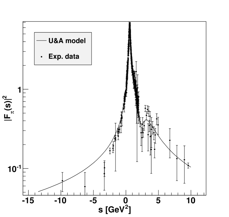
Figure 3.6: Description of pion FF data by three resonance $U\&A$ model

A description of all existing data by means of the most accomplished up to now $U\&A$ pion EM FF model (3.3) with (3.3) and (3.3), and the found values of parameters

$$\begin{array}[]{lcl}t_{in}=(1.296\pm 0.011){\rm GeV}^{2}&&R=0.0123\pm 0.0032\\ W_{z}=0.3722\pm 0.0008&&W_{p}=0.5518\pm 0.0003\\ m_{\rho}=(759.26\pm 0.04)\,{\rm MeV}&&\Gamma_{\rho}=(141.90\pm 0.13)\,{\rm MeV}\\ m_{\rho^{\prime}}=(1395.9\pm 54.3)\,{\rm MeV}&&\Gamma_{\rho^{\prime}}=(490.9\pm 118.8)\,{\rm MeV}\\ m_{\rho^{\prime\prime}}=(1711.5\pm 63.6)\,{\rm MeV}&&\Gamma_{\rho^{\prime\prime}}=(369.5\pm 112.7)\,{\rm MeV}\\ (f_{\rho\pi\pi}/f_{\rho})=1.0063\pm 0.0024&&\chi^{2}/{\rm NDF}=1.58\\ \end{array}$$

is presented in Fig. 3.6. A prediction of $\delta_{\pi}(t)$ behavior by this $U\&A$ model and its comparison with data on $\delta^{1}_{1}(t)$ is shown in Fig. 3.7.

Figure 3.7: P-wave isovector $\pi\pi$ phase shift.

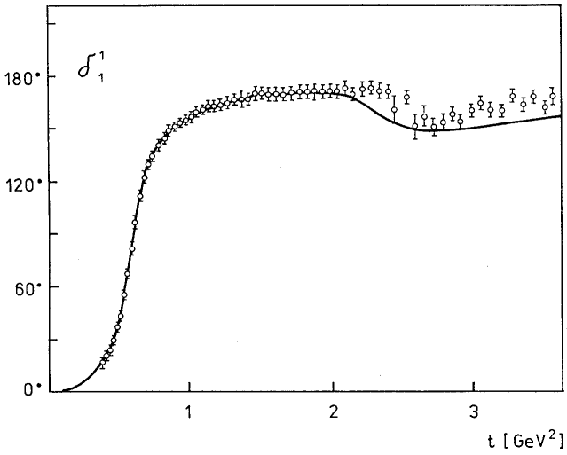
Figure 3.8: P-wave isovector $\pi\pi$ phase shift predicted by U&A model

Just the coincidence of the predicted behavior of $\delta_{\pi}(t)$ with existing data on $\delta^{1}_{1}(t)$ confirms that the $U\&A$ pion EM FF model (3.3) with (3.3) and (3.3) fulfills the unitarity condition (3.18), at least from $4m^{2}_{\pi}$ to aproximatelly $1{{\rm GeV}}^{2}$.

3.4 Prediction of P-wave isovector $\pi\pi$ phase shift and inelasticity above inelastic threshold from $e^{+}e^{-}\to\pi^{+}\pi^{-}$ process

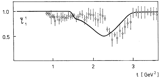
Figure 3.9: Predicted behavior of inelasticity of the P- wave

The unitary and analytic model (3.3) of $F^{E}_{\pi}[W(t)]$ has one elastic cut $4m^{2}_{\pi}<s<+\infty$ and one effective cut $t_{in}\approx 1{\rm{{\rm GeV}}}^{2}<t<+\infty$.

The elastic unitarity condition (3.18) can be utilized for the analytic continuation of $F^{E}_{\pi}[W(t)]$ through the elastic cut on the second Riemann sheet and as a result one obtains (3.26), the FF on the II. sheet to be expressed by FF on the I. sheet and the $\pi\pi$ partial wave amplitude $A^{1}_{1}(t)$ on the I. sheet, from where one obtains

$$\left[A^{1}_{1}(t)\right]^{\rm I}=\frac{\left[F^{E}_{\pi}(t)\right]^{\rm I}-\left[F^{E}_{\pi}(t)\right]^{\rm II}}{2i\left[F^{E}_{\pi}(t)\right]^{\rm II}}$$ (3.73)

to be valid in the whole complex $t$-plane.

Now, substituting a standard parametrization of I=J=1 $\pi\pi$ scattering amplitude at the physical region

$$A^{1}_{1}(t+i\varepsilon)=\frac{\eta^{1}_{1}(t+i\varepsilon)\quad{\rm e}^{2i\delta^{1}_{1}(t+i\varepsilon)}-1}{2i}$$ (3.74)

into (3.73), one gets

$$\eta^{1}_{1}(t+i\varepsilon){\rm e}^{2i\delta^{1}_{1}(t+i\varepsilon)}=\frac{\left[F^{E}_{\pi}[W(t+i\varepsilon)]\right]^{\rm I\hphantom{I}}}{\left[F^{E}_{\pi}[W(t+i\varepsilon)]\right]^{\rm II}}$$ (3.75)

from where it is straightforward to find

$$\delta^{1}_{1}(t+i\varepsilon)=\frac{1}{2}{\rm arctg}\frac{{\rm Im}\quad\frac{\left[F^{E}_{\pi}[W(t+i\varepsilon)]\right]^{\rm I\hphantom{I}}}{\left[F^{E}_{\pi}[W(t+i\varepsilon)]\right]^{\rm II}}}{{\rm Re}\quad\frac{\left[F^{E}_{\pi}[W(t+i\varepsilon)]\right]^{\rm I\hphantom{I}}}{\left[F^{E}_{\pi}[W(t+i\varepsilon)]\right]^{\rm II}}};\quad\quad\quad\eta^{1}_{1}(t+i\varepsilon)=\left|\frac{\left[F^{E}_{\pi}[W(t+i\varepsilon)]\right]^{\rm I\hphantom{I}}}{\left[F^{E}_{\pi}[W(t+i\varepsilon)]\right]^{\rm II}}\right|.$$ (3.76)

Substituting the $U\&A$ model (3.3) of the pion EM FF with (3.3), (3.3), (3.26) and (3.73) into (3.76) one predicts [51] behavior of $\delta^{1}_{1}(t+i\varepsilon)$ and $\eta^{1}_{1}(t+i\varepsilon)$ in a perfect agreement with existing data (see Figs. 3.8 and  3.9) also in the inelastic region, i.e. above 1 GeV².

The latter is clear demonstration of the analyticity as one of the powerful means in the elementary particle physics phenomenology.

3.5 Excited states of the $\rho$(770)-meson

Here we demonstrate another example of the utilization of the analyticity as the powerful means in the elementary particle physics phenomenology.

From Fig. 3.5, where the data on the pion EM FF are collected, one can see dominating role of the $\rho(770)$-meson. Besides the latter one can notice in the data also another explicit resonance around the energy $s=2.9$ GeV². But it does not mean that there are no more other hidden $\rho$-resonances in the pion EM FF to be cowered in shadow of some other resonances and the background. In such case it is difficult to identify the resonance by the Breit-Wiegner form. Here the $U\&A$ pion EM FF model, providing one analytic function in the whole interval of definition, is starting to be very suitable. So, the correct approach in an investigation of the latter problem is then to take the expression (3.3), first, with two resonances, then with three resonances etc. and to look always for minimal value of $\chi^{2}$ in experimental data fit.

Such program has been practically realized. Considering only two resonances in (3.3), $\chi^{2}/{\rm NDF}$ = 539/279 was achieved and $\rho(770)$ with $\rho^{\prime\prime}(1700)$ were identified.

However, if three resonances were taken into account in (3.3), $\chi^{2}/{\rm NDF}$ = 382/276 was found and two excited states, $\rho^{\prime}(1450)$ and $\rho^{\prime\prime}(1700)$, were identified [52].

Figure 3.10: Description of pion FF data by four resonance $U\&A$ model

Finally, by a consideration of four resonances in (3.3), $\chi^{2}/{\rm NDF}$ = 343/273 was reached and in addition to $\rho^{\prime}(1450)$ and $\rho^{\prime\prime}(1700)$, also the third excited state $\rho^{\prime\prime\prime}(2150)$ of the $\rho(770)$-meson was revealed [53] (see Fig. 3.10).

3.6 Unitary and analytic model for kaon electromagnetic structure

Unlike the pion EM FF, little has been done theoretically for the kaon EM FFs $F^{E}_{K^{+}}(t)$ and $F^{E}_{K^{0}}(t)$ up to now. The main reason was, first, the existence of a rather broad unphysical region $0<t$ $<4m^{2}_{K}$ unattainable experimentally, in which the dominating resonances $\rho(770)$, $\omega(783)$ and $\phi(1020)$ of the kaon EM FFs are spread out, and secondly, shortage of reliable and compact experimental information outside the internal $0<t$ $<4m_{K}^{2}$.

For instance, there are no data on the neutral kaon in the space-like ($t<0$) region, and for the charge kaon only 25 experimental points in the very narrow interval of momenta $-0.1145\quad{{\rm GeV}}^{2}$ $\leq t\leq-0.0175\quad{{\rm GeV}}^{2}$ exist [54, 55]. Slightly better situation is in the time-like ($t>4m^{2}_{K}$) region, where the data by means of the $e^{+}e^{-}\to K^{+}K^{-}$ and $e^{+}e^{-}\to K_{L}K_{S}$ processes have been obtained up to $t=4.5\,{{\rm GeV}}^{2}$.

The most successful description of this experimental information on the kaon EM FFs was achieved [53, 56] in the framework of the $U\&A$ model (3) to be applied to the isoscalar and isovector parts of the kaon EM FFs

$$F_{K}^{s}(t) = \left(\frac{1-V^{2}}{1-V_{N}^{2}}\right)^{2}\times$$

$$\times \left[\sum_{s=\omega,\phi}\frac{(V_{N}-V_{s})(V_{N}-V_{s}^{*})(V_{N}-1/V_{s})(V_{N}-1/V_{s}^{*})}{(V-V_{s})(V+V_{s})(V-1/V_{s})(V+1/V_{s})}(f_{sK\bar{K}}/f_{s})+\right.$$

$$+ \left.\frac{(V_{N}-V_{\phi^{\prime}})(V_{N}-V_{\phi}^{*})(V_{N}+V_{\phi^{\prime}})(V_{N}+V_{\phi^{\prime}}^{*})}{(V-V_{\phi^{\prime}})(V-V_{\phi^{\prime}}^{*})(V+V_{\phi^{\prime}})(V+V_{\phi^{\prime}}^{*})}(f_{\phi^{\prime}K\bar{K}}/f_{\phi^{\prime}})\right]$$

$$F_{K}^{v}(t) = \left(\frac{1-W^{2}}{1-W_{N}^{2}}\right)^{2}\times$$

$$\times \left[\sum_{v=\rho,\rho^{\prime}}\frac{(W_{N}-W_{v})(W_{N}-W_{v}^{*})(W_{N}-1/W_{v})(W_{N}-1/W_{v}^{*})}{(W-W_{v})(W-W_{v}^{*})(W-1/W_{v})(W-1/W_{v}^{*})}(f_{vK\bar{K}}/f_{v})+\right.$$

$$+ \left.\frac{(W_{N}-W_{\rho^{\prime\prime}})(W_{N}-W_{\rho^{\prime\prime}}^{*})(W_{N}+W_{\rho^{\prime\prime}})(W_{N}+W_{\rho^{\prime\prime}}^{*})}{(W-W_{\rho^{\prime\prime}})(W-W_{\rho^{\prime\prime}}^{*})(W+W_{\rho^{\prime\prime}})(W+W_{\rho^{\prime\prime}}^{*})}(f_{\rho^{\prime\prime}K\bar{K}}/f_{\rho^{\prime\prime}})\right],$$

which are related to the charge and neutral kaon EM FFs by the relations

$$F^{E}_{K^{+}}(t)=F^{s}_{K}(t)+F^{v}_{K}(t)$$ (3.78)

$$F^{E}_{K^{0}}(t)=F^{s}_{K}(t)-F^{v}_{K}(t)$$ (3.79)

as it follows directly from (2.7) and (2.8).

The expressions (3.6) are analytic functions in the whole $t$-plane besides two cuts on the positive real axis starting, in the case of $F_{K}^{s}(t)$ from $t_{0}^{s}=9m^{2}_{\pi}$ and $t_{in}^{s}$ and in the case of the $F_{K}^{v}(t)$ from $t_{0}^{v}=4m_{\pi}^{2}$ and $t_{in}^{v}$, to be real on the whole negative real axis up to positive values $t_{0}^{s}=9m^{2}_{\pi}$ and $t_{0}^{v}=4m^{2}_{\pi}$, respectively, automatically normalized (2.9) if

$$\sum_{s}(f_{sK\bar{K}}/f_{s})=\sum_{v}(f_{vK\bar{K}}/f_{v})=1/2,$$ (3.80)

with $ImF_{K}^{s}(t)\neq 0$ starting from $9m^{2}_{\pi}$ up to $+\infty$ and $ImF_{K}^{v}(t)\neq 0$ starting from $4m^{2}_{\pi}$ up to $+\infty$, with poles corresponding to vector-mesons placed in the complex conjugate pairs on the unphysical sheets of the Riemann surface, on which both EM FFs $F_{K}^{s}(t)$ and $F_{K}^{v}(t)$ are defined and governing the asymptotic behavior (2.24) with $n_{q}=2$ as predicted by the quark model of hadrons.

The reproduction of all existing data on $|F_{K^{+}}(t)|$ and $|F_{K^{0}}(t)|$ by means of (3.6), (3.78), (3.79) and the free parameters of the model (the values of parameters $m_{\rho}$, $\Gamma_{\rho}$, $m_{\omega}$, $\Gamma_{\omega}$ are fixed at the world averaged values)

$$\begin{array}[]{lcl}q_{in}^{s}=\sqrt{(t_{in}^{s}-9)/9}=2.2326[m_{\pi}]&&q_{in}^{v}=\sqrt{(t_{in}^{v}-4)/4}=6.6721[m_{\pi}]\\ (f_{\omega K\bar{K}}/f_{\omega})=0.14194&&(f_{\rho K\bar{K}}/f_{\rho})=0.5615\\ m_{\phi}=7.2815[m_{\pi}]&&m_{\rho^{\prime}}=10.3940[m_{\pi}]\\ \Gamma_{\phi}=0.03733[m_{\pi}]&&\Gamma_{\rho^{\prime}}=1.6284[m_{\pi}]\\ (f_{\phi K\bar{K}}/f_{\phi})=0.4002&&(f_{\rho^{\prime}K\bar{K}}/f_{\rho^{\prime}})=-0.3262\\ m_{\phi^{\prime}}=11.8700[m_{\pi}]&&m_{\rho^{\prime\prime}}=13.5650[m_{\pi}]\\ \Gamma_{\phi^{\prime}}=1.3834[m_{\pi}]&&\Gamma_{\rho^{\prime\prime}}=3.4313[m_{\pi}]\\ (f_{\phi^{\prime}K\bar{K}}/f_{\phi^{\prime}})=-.04214&&(f_{\rho^{\prime\prime}K\bar{K}}/f_{\rho^{\prime\prime}})=-.02888\\ \chi^{2}/{\rm NDF}=181/166&&\end{array}$$ (3.81)

are presented in Fig. 3.11.

Figure 3.11: Description of the charged and neutral kaon FF data by $U\&A$ model.

From the obtained results one observes that the contribution of the $\rho^{\prime\prime\prime}(2150)$ resonance to the $e^{+}e^{-}\to K\bar{K}$ processes is favored prior to the $\rho^{\prime\prime}(1700)$ one by the existing data in the charge and neutral kaon EM FFs.

In the Review of Particle Properties [12] are besides $\omega(783)$ meson also its higher excitation states, $\omega(1420)$ and $\omega(1600)$, presented. Therefore it could be interesting to investigate their contributions to the $e^{+}e^{-}\to K\bar{K}$ processes by means of the $U\&A$ model of the kaon Em FFs.

However, the latter problem can be considered seriously only in the case that more abundant and more precise experimental information on the kaon EM FFs will appear.

3.7 Conserved-vector-current (CVC) hypothesis and the $\bar{\nu}_{e}e\to M^{-}M^{0}$ and $\tau^{-}\to\nu_{\tau}M^{-}M^{0}$ weak processes

At the end of fifties, by Gerstein and Zeldowich [57], and independently by Feynman and Gell-Mann [58], the conserved-vector-current (CVC) hypothesis, as a theoretical ground for an explanation of an approximate numerical equality of the muon decay constant $G_{\mu}$ and the neutron decay vector constant $G_{\rm V}$, was postulated in the framework of the V-A weak interaction theory.

The latter hypothesis, besides others, provides a relation between a matrix element of the vector part of the weak charged hadronic current and a corresponding matrix element of the EM current to be taken between two pion states. As a result of the foregoing, a probability of the $\pi^{+}$-meson beta-decay $\pi^{+}\to\pi^{0}+e^{+}+{\nu}_{e}$ was predicted [57, 58] theoretically. Its agreement with experimental results was presented [59] as a demonstration of the general validity of the CVC hypothesis in the weak interaction theory.

Further, based on the CVC hypothesis and $U\&A$ model of the pseudoscalar meson EM FF’s formulated above, we predict [60],[61] a behavior of $\sigma_{\rm tot}(E^{\rm lab}_{\nu})$ and d$\sigma$/d$E^{\rm lab}_{\pi}$ of the weak $\bar{\nu}_{\rm e}e^{-}\to M^{-}M^{0}$ processes for the first time and the ratio of total probabilities $\Gamma(\tau^{-}\to\bar{\nu}_{\tau}M^{-}M^{0})/\Gamma_{e}$ are determined and compared with experimental values and theoretical values of other estimates.

In general, the differential cross-section of the weak $\bar{\nu}_{e}e^{-}\to M^{-}M^{0}$ reactions in the c.m. system is given by the following expression

$$\frac{{\rm d}\sigma}{{\rm d}{\mit\Omega}}=\frac{1}{(2\mbox{s}_{\bar{\nu}}+1)(2\mbox{s}_{\rm e}+1)}\frac{1}{64\pi^{2}s}\frac{k^{\rm c.m.}}{p^{\rm c.m}}\sum_{\mbox{s}_{\bar{\nu}},\mbox{s}_{e}}|{\cal{M}}|^{2},$$ (3.82)

where $s\geq 4m_{\pi}^{2}$ is the c.m. energy squared, $k^{\rm c.m.}=[(s-4m_{\pi}^{2})/4]^{1/2}$ is a length of a 3-dimensional momentum of produced pseudoscalar mesons, $p^{\rm c.m.}=\sqrt{s/4}$ is a length of a 3-dimensional neutrino-momentum (assuming $m_{\nu_{\rm e}}=0$) and $s_{\bar{\nu}}$ and $s_{\rm e}$ are spins of the antineutrino and electron, respectively. The matrix element $M$ in the lowest order of a perturbation expansion can be calculated from the Feynman diagram presented in Fig. 3.12a (the $F_{M}^{\rm W}(s)$ is the weak FF of a charged $W^{-}$-boson transition $(W^{-})^{*}\to M^{-}M^{0}$), which for $s\ll m_{{\rm W}^{-}}^{2}$ is reduced to a contact diagram shown in Fig. 3.12b.

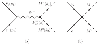
Figure 3.12: Reduction of the Feynman diagram to contact one

In the standard electro-weak theory an effective Hamiltonian describing the $\bar{\nu}_{\rm e}e^{-}\to M^{-}M^{0}$ process is

$${\cal H}_{\rm I}=\frac{G}{\sqrt{2}}\left[\bar{\nu}_{\rm e}\gamma_{\mu}\left(1+\gamma_{5}\right)e\right]J_{\mu}^{W}+h.c.,$$ (3.83)

where $G=1.1663\times 10^{-5}\mbox{\,{{\rm GeV}}}^{-2}$ is the Fermi constant of the weak interactions and $J_{\mu}^{W}$ is a pseudoscalar meson weak current. Then the matrix element corresponding to the diagrams in Fig. 3.12 takes the form

$${\cal M}=\frac{G}{\sqrt{2}}\bar{\nu}_{\rm e}(p_{2})\gamma_{\mu}\left(1+\gamma_{5}\right)e(p_{1})\left(k_{1}-k_{2}\right)^{\mu}F_{M}^{\rm W}(s)$$ (3.84)

and as a result, the differential cross-section (3.82) can be calculated explicitly

$$\frac{{\rm d}\sigma}{{\rm d}{\mit\Omega}}=\frac{G^{2}}{128\pi^{2}}\cdot s\beta^{3}_{M}|F^{\rm W}_{M}(s)|^{2}\sin^{2}{\vartheta},$$ (3.85)

where $\beta_{M}=\sqrt{1-4m^{2}_{M}/s}$ is the velocity of produced pions and $\vartheta$ is the scattering angle in the c.m. system.

Now considering an explicit form of d$\mit\Omega$=$\sin\vartheta$ d$\vartheta$ d$\varphi$ and then integrating over angles $\vartheta$ and $\varphi$ in (3.85), one gets the total cross-section

$$\sigma_{\rm tot}(s)=\frac{G^{2}}{48\pi}s\cdot\beta_{M}^{3}|F_{M}^{\rm W}(s)|^{2}$$ (3.86)

of the weak $\bar{\nu}_{\rm e}e^{-}\to M^{-}M^{0}$ process.

In order to predict the behavior of (3.85) or (3.86) as dependent on $s$, one is in need of a knowledge of the weak pion FF $F_{M}^{\rm W}(s)$ as a function of $s$. Since, there are neither data on the latter, nor accomplished dynamical theory of strong interactions able to predict the $F_{M}^{\rm W}(s)$ behavior for $s\geq 4m_{M}^{2}$, not even a phenomenological approach like it is in the case of the EM FF’s, one has to use the CVC-hypothesis [57, 58] providing a relation of the weak $F_{M}^{\rm W}(s)$ just with the pure isovector part of EM FF’s of the pseudoscalar mesons.

In order to derive the latter relations we start with the standard expression of the pseudoscalar meson weak current

$$J^{\rm W}_{\mu}=V_{\mu}+A_{\mu}$$ (3.87)

where $V_{\mu}$ and $A_{\mu}$ are the vector and axial-vector, respectively.

On the other hand, the EM current of hadrons is composed of the sum

$$J^{\rm E}_{\mu}=(J_{3})_{\mu}+(J_{\rm S})_{\mu},$$ (3.88)

where $(J_{3})_{\mu}$ is a third component of an isotopic vector current $\vec{J}^{\mu}(J_{1}^{\mu},J_{2}^{\mu},J_{3}^{\mu})$ and $(J_{\rm S})0_{\mu}$ is an isoscalar current.

In the second-half of the fifties a very predictable postulation was introduced

$$V^{\mu}=J_{1}^{\mu}-iJ_{2}^{\mu},$$ (3.89)

i.e. that the charged weak vector current $V^{\mu}$ and the isovector part $J_{3}^{\mu}$ of the EM current are components of the same isotopic vector $\vec{J}^{\mu}$. Since, strong interactions are invariant with respect to the isotopic SU(2) group, the isotopic vector current $\vec{J}^{\mu}$ obeys the relation

$$\partial_{\mu}J_{i}^{\mu}=0,$$ (3.90)

which directly results in the formalism of the conserved-vector-current (CVC) hypothesis

$$\partial_{\mu}V^{\mu}=0.$$ (3.91)

Further, in order to derive a relation between $F_{M}^{\rm W}(s)$ and $F_{M}^{\rm E,I=1}(s)$, we start with a commutation relation

$$\left[T_{i},J^{\mu}_{j}\right]=i\varepsilon_{ijk}J_{k}^{\mu},$$ (3.92)

with $T_{i}$ being an isospin operator. The relation (3.92) is fulfilled automatically if $\vec{J}^{\mu}$ is transformed in the isospin space like a vector. Now defining

$$T_{-}=T_{1}-i\,T_{2}$$

and (3.93)

$$J^{\mu}_{-}=J_{1}^{\mu}-i\,J_{2}^{\mu},$$

one can prove the following relation

$$\left[T_{-},J_{3}^{\mu}\right]=J_{-}^{\mu}\,\equiv\,V^{\mu}$$ (3.94)

by using expressions (3.93).

If we multiply (3.94) from the right-hand side by a state vector of $M^{+}$ pseudoscalar meson $|M^{+}\rangle$ and from the left-hand side by a state vector of $M^{0}$ pseudoscalar meson $\langle M^{0}|$ of the same isomultiplet, and simultaneously we use the relations

$$T_{-}|T,T_{3}\rangle = \sqrt{(T+T_{3})(T-T_{3}+1)}\quad|T,T_{3}-1\rangle$$ (3.95)

$$\langle T,T_{3}|T_{-} = \sqrt{(T-T_{3})(T+T_{3}+1)}\quad\langle T,T_{3}+1|$$

we get

$$\langle M^{0}|V^{\mu}|M^{+}\rangle=\langle M^{0}|\left[T_{-},J^{\mu}_{3}\right]|M^{+}\rangle=$$ (3.96)

$$=\sqrt{(T-T_{3})(T+T_{3}+1)}\quad\langle M^{+}|J^{\mu}_{3}|M^{-}\rangle-\sqrt{(T+T_{3})(T-T_{3}+1)}\quad\langle M^{0}|J^{\mu}_{3}|M^{0}\rangle.$$

Then from (3.96) for pions one gets the relations as follows

$$\langle\pi^{0}|V^{\mu}|\pi^{+}\rangle=\sqrt{2}\langle\pi^{+}|J^{\mu}_{3}|\pi^{+}\rangle-\sqrt{2}\langle\pi^{0}|J^{\mu}_{3}|\pi^{0}\rangle,$$ (3.97)

in which the second term is zero due to the charge conjugation. Really, if $U_{\rm C}$ is a unitary charge conjugation operator, and

$$U_{\rm C}|\pi^{0}\rangle=|\pi^{0}\rangle,\quad\quad\quad U_{\rm C}J^{\mu}_{3}U_{\rm C}^{-1}=-J^{\mu}_{3},$$ (3.98)

then

$$\langle\pi^{0}|J_{3}^{\mu}|\pi^{0}\rangle=\langle\pi^{0}|U_{\rm C}^{-1}U_{\rm C}J^{\mu}_{3}U_{\rm C}^{-1}U_{\rm C}|\pi^{0}\rangle=-\langle\pi^{0}|J^{\mu}_{3}|\pi^{0}\rangle\equiv 0.$$ (3.99)

So, finally one gets the relation

$$\langle\pi^{0}|V^{\mu}|\pi^{+}\rangle=\sqrt{2}\langle\pi^{+}|J^{\mu}_{3}|\pi^{+}\rangle.$$ (3.100)

On the other hand, if we multiply (3.88) from the right-hand side and left-hand side by a state vector of $\pi^{+}$ meson, we get

$$\langle\pi^{+}|J^{\mu}_{\rm E}|\pi^{+}\rangle=\langle\pi^{+}|J^{\mu}_{3}|\pi^{+}\rangle\,+\,\langle\pi^{+}|J^{\mu}_{S}|\pi^{+}\rangle.$$ (3.101)

Because strong interactions are invariant under the G-transformation, that is a combination of the charge conjugation and an isotopic rotation for an angle 180^∘ around the second axis in the isospin space, the second term in (3.101) is equal to zero. Really, considering that

$$U_{\rm G}|\pi^{+}\rangle=-|\pi^{+}\rangle,\makebox[85.35826pt]{ }U_{\rm G}J^{\mu}_{\rm S}U_{\rm G}^{-1}=-J^{\mu}_{\rm S}$$ (3.102)

one has

$$\langle\pi^{+}|J_{\rm S}^{\mu}|\pi^{+}\rangle=\langle\pi^{+}|U_{\rm G}^{-1}U_{\rm G}J^{\mu}_{S}U_{\rm G}^{-1}U_{\rm G}|\pi^{+}\rangle=-\langle\pi^{+}|J^{\mu}_{\rm S}|\pi^{+}\rangle\equiv 0$$ (3.103)

and as a result,

$$\langle\pi^{+}|J_{\rm E}^{\mu}|\pi^{+}\rangle=\langle\pi^{+}|J^{\mu}_{3}|\pi^{+}\rangle.$$ (3.104)

Comparison of (3.104) with (3.100) leads to

$$\langle\pi^{0}|V^{\mu}|\pi^{+}\rangle=\sqrt{2}\langle\pi^{+}|J^{\mu}_{\rm E}|\pi^{+}\rangle.$$ (3.105)

Then parametrizing the matrix elements in (3.105) through corresponding FF’s one gets finally the relation between the pure isovector part of the pion EM FF and the weak pion FF in the following form

$$F_{\pi}^{\rm W}(s)=\sqrt{2}F_{\pi}^{\rm E,I=1}(s).$$ (3.106)

For kaons the expression (3.96) gives the following relation

$$\langle K^{0}|V^{\mu}|K^{+}\rangle=\langle K^{+}|J^{\mu}_{3}|K^{+}\rangle-\langle K^{0}|J^{\mu}_{3}|K^{0}\rangle.$$ (3.107)

By using the relation (3.88) one can write down for the difference

$$\langle K^{+}|J^{\mu}_{E}|K^{+}\rangle-\langle K^{0}|J^{\mu}_{E}|K^{0}\rangle=$$

$$= \langle K^{+}|J^{\mu}_{3}|K^{+}\rangle-\langle K^{0}|J^{\mu}_{3}|K^{0}\rangle+\langle K^{+}|J^{\mu}_{S}|K^{+}\rangle-\langle K^{0}|J^{\mu}_{S}|K^{0}\rangle.$$

Now applying the relations

$$T_{+}|T,T_{3}\rangle = \sqrt{(T-T_{3})(T+T_{3}+1)}\quad|T,T_{3}+1\rangle$$ (3.109)

$$\langle T,T_{3}|T_{+} = \sqrt{(T+T_{3})(T-T_{3}+1)}\quad\langle T,T_{3}-1|$$

to kaons as follows

$$T_{+}|K^{0}\rangle=|K^{+}\rangle;\quad\quad\quad\langle K^{+}|T_{+}=\langle K^{0}|$$ (3.110)

one gets

$$\langle K^{+}|J^{\mu}_{S}|K^{+}\rangle=\langle K^{+}|J^{\mu}_{S}T_{+}|K^{0}\rangle=\langle K^{+}|T_{+}J^{\mu}_{S}|K^{0}\rangle=\langle K^{0}|J^{\mu}_{S}|K^{0}\rangle$$ (3.111)

which in (3.7) leads to

$$\langle K^{+}|J^{\mu}_{E}|K^{+}\rangle-\langle K^{0}|J^{\mu}_{E}|K^{0}\rangle=\langle K^{+}|J^{\mu}_{3}|K^{+}\rangle-\langle K^{0}|J^{\mu}_{3}|K^{0}\rangle.$$ (3.112)

A comparison of (3.107) and (3.112) gives finally

$$\langle K^{0}|V^{\mu}|K^{+}\rangle=\langle K^{+}|J^{\mu}_{E}|K^{+}\rangle-\langle K^{0}|J^{\mu}_{E}|K^{0}\rangle.$$ (3.113)

Then parametrizing the matrix elements in (3.112) through corresponding FF’s, we obtain the relation between the isovector part of the kaon EM FF’s and the weak kaon FF in the following form

$$F_{K}^{W}(s)=F_{K^{+}}(s)-F_{K^{0}}(s)=F_{K}^{S}(s)+F_{K}^{V}(s)-F_{K}^{S}(s)+F_{K}^{V}(s)=2F_{K}^{V}(s).$$ (3.114)

Substituting the relations (3.106) and (3.114) into (3.85) and (3.86) and using the unitary and analytic model of the pion and kaon EM structure formulated in we get the differential and total cross-sections

$$\frac{{\rm d}\sigma(\bar{\nu}_{e}e^{-}\to\pi^{-}\pi^{0})}{{\rm d}\Omega}=\frac{G^{2}}{64\pi^{2}}\beta^{3}_{\pi}\cdot s|F^{\rm E,I=1}_{\pi}(s)|^{2}\sin^{2}{\vartheta}$$ (3.115)

$$\sigma_{\rm tot}(\bar{\nu}_{e}e^{-}\to\pi^{-}\pi^{0})=\frac{G^{2}}{24\pi}\beta^{3}_{\pi}\cdot s|F_{\pi}^{\rm E,I=1}(s)|^{2}$$ (3.116)

and

$$\frac{{\rm d}\sigma(\bar{\nu}_{e}e^{-}\to K^{-}K^{0})}{{\rm d}\Omega}=\frac{G^{2}}{32\pi^{2}}\beta^{3}_{K}\cdot s|F^{V}_{K}(s)|^{2}\sin^{2}{\vartheta}$$ (3.117)

$$\sigma_{\rm tot}(\bar{\nu}_{e}e^{-}\to K^{-}K^{0})=\frac{G^{2}}{12\pi}\beta^{3}_{K}\cdot s|F_{K}^{V}(s)|^{2}$$ (3.118)

of the weak annihilation processes $\bar{\nu}_{\rm e}e^{-}\to\pi^{-}\pi^{0}$ and $\bar{\nu}_{\rm e}e^{-}\to K^{-}K^{0}$ respectively, for the first time [60, 61]. The comparison of $\sigma_{\rm tot}(\bar{\nu}_{\rm e}e^{-}\to\pi^{-}\pi^{0})$ with $\sigma_{\rm tot}(e^{+}e^{-}\to\pi^{+}\pi^{-})$, and comparison of $\sigma_{\rm tot}(\bar{\nu}_{\rm e}e^{-}\to K^{-}K^{0})$ with $\sigma_{\rm tot}(e^{+}e^{-}\to K^{+}K^{-})$ and $\sigma_{\rm tot}(e^{+}e^{-}\to K^{0}_{S}K^{0}_{L})$ is presented in Fig. 3.13 and Fig. 3.14, respectively.

Figure 3.13: Cross-section comparison of electromagnetic and weak process.

Figure 3.14: Cross-section comparison of electromagnetic and weak process.

However, the results in Fig. 3.13 and Fig. 3.14 are not very interesting for experimentalists because the weak annihilation process $\bar{\nu}_{\rm e}e^{-}\to M^{-}M^{0}$ can be in principle measured only in an interaction of antineutrino beams with atomic electrons in the laboratory system.

The corresponding total cross-sections in the laboratory system can be found by using the following relation

$$s=m^{2}_{\rm e}+2m_{\rm e}\;E_{\nu}^{\rm lab}$$ (3.119)

which leads to the expressions

$$\sigma_{\rm tot}^{lab}(\bar{\nu}_{\rm e}e^{-}\to\pi^{-}\pi^{0})=\frac{G^{2}}{24\pi}(m_{\rm e}^{2}+2m_{\rm e}E_{\nu}^{\rm lab})\beta^{3}_{\pi}|F_{\pi}^{\rm E,I=1}(E_{\nu}^{\rm lab})|^{2}$$ (3.120)

and

$$\sigma_{\rm tot}^{lab}(\bar{\nu}_{\rm e}e^{-}\to K^{-}K^{0})=\frac{G^{2}}{12\pi}(m_{\rm e}^{2}+2m_{\rm e}E_{\nu}^{\rm lab})\beta^{3}_{K}|F_{K}^{V}(E_{\nu}^{\rm lab})|^{2},$$ (3.121)

respectively.

It is also interesting to have a prediction of the energy distribution of the pseudoscalar mesons created in the final state of the weak $\bar{\nu}_{\rm e}e^{-}\to M^{-}M^{0}$ process given by the differential cross-section d$\sigma/{\rm d}E_{M}^{\rm lab}$ in the laboratory system. With this aim we use in (3.115) and (3.117) the explicit form of d${\mit\Omega}=-{\rm d}\cos\vartheta\quad{\rm d}\varphi$ and integrate the corresponding expressions over the angle $\varphi$. Then we insert

$${\rm d}\cos\vartheta = -\frac{m_{\rm e}}{k^{\rm c.m.}p^{\rm c.m.}}{\rm d}E_{M}^{\rm lab};\quad\quad\quad\quad s\approx 2m_{\rm e}E_{\nu}^{\rm lab};$$ (3.122)

$$\sin^{2}\vartheta = 1-\frac{(E_{M}^{\rm c.m.}E_{\rm e}^{\rm c.m.}-m_{\rm e}E_{M}^{\rm lab})^{2}}{(k^{\rm c.m.})^{2}(p^{\rm c.m.})^{2}},$$ (3.123)

where

$$E_{M}^{\rm c.m}\approx E_{\rm e}^{\rm c.m.}\approx p^{\rm c.m}\approx\sqrt{{m_{\rm e}\over 2}E_{\nu}^{\rm lab}};\quad\quad\quad\quad\mbox{and}\quad\quad\quad k^{\rm c.m.}\approx\sqrt{{m_{\rm e}\over 2}(E_{\nu}^{\rm lab}-E_{\nu}^{(0)})}$$ (3.124)

with the threshold energy $E_{\nu}^{(0)}=(4m_{M}^{2}-m_{e}^{2})/2m_{e}$ of the antineutrino beam to be $E_{\nu\pi}^{(0)}=76.7\,{{\rm GeV}}$ for pions and $E_{\nu K}^{(0)}=962\,{{\rm GeV}}$ for kaons. As a result, the following expressions for the energy distributions of pions and kaons

$$\frac{{\rm d}\sigma(\bar{\nu}_{\rm e}e^{-}\to\pi^{-}\pi^{0})}{{\rm d}E_{\pi}^{\rm lab}}=\frac{m_{\rm e}G^{2}}{8\pi}\left(\frac{E_{\nu}^{\rm lab}-E_{\nu\pi}^{(0)}}{E_{\nu}^{\rm lab}}\right)\left\{1-\frac{(E_{\nu}^{\rm lab}-2E_{\pi}^{\rm lab})^{2}}{E_{\nu}^{\rm lab}(E_{\nu}^{\rm lab}-E_{\nu\pi}^{(0)})}\right\}|F_{\pi}^{\rm E,I=1}(E_{\nu}^{\rm lab})|^{2}$$ (3.125)

and

$$\frac{{\rm d}\sigma(\bar{\nu}_{\rm e}e^{-}\to K^{-}K^{0})}{{\rm d}E_{K}^{\rm lab}}=\frac{m_{\rm e}G^{2}}{4\pi}\left(\frac{E_{\nu}^{\rm lab}-E_{\nu K}^{(0)}}{E_{\nu}^{\rm lab}}\right)\left\{1-\frac{(E_{\nu}^{\rm lab}-2E_{K}^{\rm lab})^{2}}{E_{\nu}^{\rm lab}(E_{\nu}^{\rm lab}-E_{\nu K}^{(0)})}\right\}|F_{K}^{V}(E_{\nu}^{\rm lab})|^{2}$$ (3.126)

are obtained, respectively.

In the last few years a considerable improvement in the detection of small exclusive hadronic tau-decay processes has been achieved. As a result, also experimental values on the branching ratio $BR(\tau^{-}\to\nu_{\tau}M^{-}M^{0})$ were obtained recently, where $M$ means a pseudoscalar meson.

In order to predict it theoretically, we start with a general expression for a probability of $\tau^{-}(k_{1})\to\nu_{\tau}(k_{2})M^{-}(p_{1})M^{0}(p_{2})$ decay process

$$d\Gamma=(2\pi)^{4}\int\frac{\bar{|}{\cal M}|^{2}}{2m_{\tau}}\delta(k_{1}-k_{2}-p_{1}-p_{2})\frac{d^{3}k_{2}}{(2\pi)^{3}2E_{\nu}}\frac{d^{3}p_{1}}{(2\pi)^{3}2E_{1}}\frac{d^{3}p_{2}}{(2\pi)^{3}2E_{2}},$$ (3.127)

where the corresponding matrix element takes the following form

$${\cal M}=\frac{G_{F}\cos{\theta_{C}}}{\sqrt{2}}\bar{u}(k_{2})\gamma_{\mu}(1+\gamma_{5})u(k_{1})J_{\mu}^{W}$$ (3.128)

and $\theta_{C}$ is the Cabibbo angle. In the expression (3.128) the $W$-boson exchange mechanism is assumed to be realized. However, since $m_{\tau}^{2}/m^{2}_{W}<<1$, all effects due to the $W$-boson exchange can be neglected. $G_{F}$ means the Fermi constant of weak interactions and $J_{\mu}^{W}$ is a matrix element of the weak charge vector current responsible for the $W^{-}\to K^{-}K^{0}$ transition.

Then the absolute value squared of the matrix element (3.128) takes the form as follows

$$|\bar{\cal M}|^{2}=\frac{G_{F}^{2}\cos^{2}{\theta_{C}}}{2}[\ell_{\mu\nu}+r_{\mu\nu}]J_{\mu}^{W}(J_{\mu}^{W})^{*}$$ (3.129)

with

$$\ell_{\mu\nu}=4[k_{1\mu}k_{2\nu}+k_{1\nu}k_{2\mu}-g_{\mu\nu}(k_{1}\cdot k_{2}]$$ (3.130)

$$r_{\mu\nu}=4i\epsilon_{\mu\nu\alpha\beta}s_{\alpha}k_{2\beta}-4m_{\tau}[s_{\mu}k_{2\nu}+s_{\nu}k_{2\mu}-g_{\mu\nu}(s\cdot k_{2})],$$

where $s$ is the $\tau$-lepton spin four-vector, $s\cdot k_{1}=0$ and the bar (3.129) means an average over the spin of the $\tau$-lepton and a summation over the spin states of the neutrino $\nu_{\tau}$.

It is straightforward to rewrite (3.127) into the following three equivalent forms

$$d\Gamma = \frac{|{\cal M}|^{2}}{64\pi^{3}}\frac{dEdE_{\nu}}{m_{\tau}},$$ (3.131)

$$d\Gamma = \frac{|{\cal M}|^{2}}{128\pi^{3}}\frac{dEdk^{2}}{m_{\tau}^{2}},$$ (3.132)

$$d\Gamma = \frac{|{\cal M}|^{2}}{256\pi^{3}}m_{\tau}dxdy,$$ (3.133)

where $E$ is the energy of the $M^{-}$ pseudoscalar meson at the $\tau$-lepton rest reference frame, $k^{2}=(k_{1}-k_{2})^{2}=m_{\tau}(m_{\tau}-2E_{\nu})$ is the effective mass squared of the $M^{-}M^{0}$ system, $x=k^{2}/m_{\tau}^{2}$ and $y=2E/m_{\tau}$.

If we define $Q=4m^{2}_{M}/m_{\tau}$, then

$$R\leq x\leq 1;\quad\quad\quad{\rm and}\quad\quad\sqrt{R}\leq y\leq 1.$$ (3.134)

The matrix element of the weak vector current of the $W^{-}\to M^{-}M^{0}$ transition can be parametrized in the following way

$$J_{\mu}^{W}=(p_{1}-p_{2})_{\mu}F_{M}^{W}(k^{2}),$$ (3.135)

where $F_{M}^{W}(k^{2})$ is the weak FF of the corresponding pseudoscalar mesons. By using (3.135), (3.129)-(3.130) and an integration over the energy of the $M^{-}$ pseudoscalar meson in (3.130) one gets the relation as follows

$$d\Gamma=\frac{G_{F}^{2}\cos^{2}{\theta_{C}}}{768\pi^{3}m_{\tau}^{3}}dk^{2}(m_{\tau}^{2}-k^{2})^{2}(m_{\tau}^{2}+2k^{2})(1-\frac{4m_{M}^{2}}{k^{2}})^{3/2}|F_{M}^{W}(k^{2})|^{2}.$$ (3.136)

Now, if instead of the weak pseudoscalar meson FF in (3.136) the EM FFs by (3.106) and (3.114) are substituted, one gets the decay widths

$$\Gamma(\tau^{-}\to\nu_{\tau}\pi^{-}\pi^{0})=\frac{G_{F}^{2}\cos^{2}{\theta_{C}}}{384\pi^{3}m_{\tau}^{3}}\int_{4m_{\pi}^{2}}^{m_{\tau}^{2}}dk^{2}(m_{\tau}^{2}-k^{2})^{2}(m_{\tau}^{2}+2k^{2})(1-\frac{4m_{\pi}^{2}}{k^{2}})^{3/2}|F_{\pi}^{I=1,E}(k^{2})|^{2}$$ (3.137)

$$\Gamma(\tau^{-}\to\nu_{\tau}K^{-}K^{0})=\frac{G_{F}^{2}\cos^{2}{\theta_{C}}}{192\pi^{3}m_{\tau}^{3}}\int_{4m_{K}^{2}}^{m_{\tau}^{2}}dk^{2}(m_{\tau}^{2}-k^{2})^{2}(m_{\tau}^{2}+2k^{2})(1-\frac{4m_{K}^{2}}{k^{2}})^{3/2}|F_{K}^{v}(k^{2})|^{2},$$ (3.138)

respectively. By using in (3.137) the pion EM FF $U\&A$ model (3.3) with the corresponding parameter values and in (3.138) the isovector part of kaon EM FF $U\&A$ model (3.6) with the corresponding parameter values (3.81), and simultaneously $G_{F}=0.2278\times 10^{-6}[m^{-2}_{\pi}]$, $\sin\theta_{C}=0.22$ we finally get the decay widths

$$\Gamma(\tau^{-}\to\nu_{\tau}\pi^{-}\pi^{0})=0.3898\times 10^{-11}[m_{\pi}]$$ (3.139)

and

$$\Gamma(\tau^{-}\to\nu_{\tau}K^{-}K^{0})=0.2574\times 10^{-13}[m_{\pi}],$$ (3.140)

respectively. Dividing the latter values by the total width of the $\tau$-lepton to be

$$\Gamma^{tot}=0.159\times 10^{-10}[m_{\pi}]$$ (3.141)

one gets the corresponding branching ratios

$$BR(\tau^{-}\to\nu_{\tau}\pi^{-}\pi^{0})=24.52\%$$

and

$$BR(\tau^{-}\to\nu_{\tau}K^{-}K^{0})=0.16\%$$

respectively. They can be compared with the recent experimental values

$$BR^{exp}(\tau^{-}\to\nu_{\tau}\pi^{-}\pi^{0})=(25.30\pm 0.20)\%$$

and

$$BR^{exp}(\tau^{-}\to\nu_{\tau}K^{-}K^{0})=(0.26\pm 0.09)\%$$

obtained by ALEPH Collaboration [62] in CERN. There is very good agreement of our theoretical predictions with experiment.

3.8 Parameter differences of the charged and neutral $\rho$-meson family

Isotopic spin is to a very good approximation the conserved quantum number in strong interactions. A breaking of the corresponding symmetry occurs as a consequence of EM interactions and the mass difference of the up and down quarks. Practically, it is demonstrated in nature by a splitting of hadrons into isomultiplets.

In this paragraph we are concerned with $\rho$-meson resonances. The cleanest determination of their parameters comes from the ${e}^{+}{e}^{-}$ annihilation and $\tau$-lepton decay. However, as it is declared by the Review of Particle Physics [12], experimental accuracy is not yet sufficient for unambiguous conclusions. The difference for $\rho^{0}$ and $\rho^{\pm}$ are presented in averaged to be $m_{\rho^{0}}-m_{\rho^{\pm}}=-0.7\pm 0.8{MeV}$ and $\Gamma_{\rho^{0}}-\Gamma_{\rho^{\pm}}=0.3\pm 1.3{MeV}$, respectively.

Nowadays the situation is changed in two aspects.

On one hand, new very accurate KLOE data [43] on the pion EM form factor (FF) at the energy range $0.35{GeV}^{2}\leq t\leq 0.95{GeV}^{2}$ were obtained by the radiative return method in Frascati. Also corrected CMD-2 [45] and SND [46] Novosibirsk ${e}^{+}{e}^{-}\to\pi^{+}\pi^{-}$ data have appeared recently.

On the other hand the weak pion FF accurate data [63] from the measurement of the $\tau^{-}\to\pi^{-}\pi^{0}\nu_{\tau}$ decay by Belle (KEK) experiment were published recently.

The $U\&A$ model (3.3) of the pion EM FF, to be represented by one analytic function for $-\infty<t<+\infty$ was elaborated, which is always successfully applied for a description of existing data on the pion EM FF from ${e}^{+}{e}^{-}\to\pi^{+}\pi^{-}$ and due to the CVC hypothesis [60] equally well also for a description of existing data on the weak pion FF from $\tau^{-}\to\pi^{-}\pi^{0}\nu_{\tau}$ decay.

As a result more sophisticated evaluation of a difference of the $\rho$-meson families parameters can be achieved [64].

For the pion EM FF there is almost continuous interval of 381 experimental points for
$-9.77{GeV}^{2}\leq t\leq 13.48{GeV}^{2}$, which all are described by the pion EM FF model (3.3) in the space-like and the time-like regions simultaneously. The most important from them are accurate KLOE data [43] at the energy range $0.35{GeV}^{2}\leq t\leq 0.95{GeV}^{2}$ obtained in Frascati by the radiative return method and also the corrected Novosibirsk CMD-2 data [45] at the range $0.36{GeV}^{2}\leq t\leq 0.9409{GeV}^{2}$ and SND data [46] at the range $0.1521{GeV}^{2}\leq t\leq 0.9409{GeV}^{2}$, which can influence the finite results substantially. They are supplemented at the interval $-9.77{GeV}^{2}\leq t\leq 0.3364{GeV}^{2}$ and $0.9557{GeV}^{2}\leq t\leq 13.48{GeV}^{2}$ by other existing data.

An application of the pion EM FF $U\&A$ model (3.3) with three lowest resonances, in order to take into account the fact that the mass of the $\tau$ lepton in decay $\tau^{-}\to\pi^{-}\pi^{0}\nu_{\tau}$ allows to reach not more than the energy corresponding just to the second radially excited state $\rho^{\prime\prime}(1700)$ meson, leads to the best description of all existing 381 experimental points with the values of the parameters presented in the second column of the Tab. 3.1.

The weak decay $\tau^{-}\to\pi^{-}\pi^{0}\nu_{\tau}$ is, like the $e^{+}e^{-}\to\pi^{+}\pi^{-}$ process, dominated by the $\rho^{-}$-meson family resonances and thus it can be used to extract information on the charged $\rho$-meson family properties.

From the conservation of vector current (CVC) theorem it follows (3.106), i.e. the $\pi^{-}\pi^{0}$ mass spectrum in the $\tau^{-}\to\pi^{-}\pi^{0}\nu_{\tau}$ decay can be related to the total cross section of the ${e}^{+}{e}^{-}\to\pi^{+}\pi^{-}$ process. As a result the same $U\&A$ pion EM FF model (3.3) can be applied to a description of the weak pion FF data, which can be drawn from the measured normalized invariant mass-spectrum.

Though there are measurements of $\tau^{-}\to\pi^{-}\pi^{0}\nu_{\tau}$ decay to be carried out previously by ALEPH [65] and CLEO [66], here we are concentrated only on the high-statistics measurement [63] of the weak pion FF from $\tau^{-}\to\pi^{-}\pi^{0}\nu_{\tau}$ decay with the Belle detector at the KEK-B asymmetric-energy ${e}^{+}{e}^{-}$ collider as they are charged by the lowest total errors.

An application of the pion EM FF $U\&A$ model (3.3) to the best description of 62 experimental points [63] on the weak pion FF leads to the values of the parameters also presented in Tab. 3.1, however, in the third column.

There may be a question about the fact that the obtained $\rho$-meson family parameters are differing from those presented at the Review of the Particle Physics [12], especially of the $\rho(770)$- and $\rho^{\prime}(1450)$-mesons. As it is well known, the resonance parameters depend on the parametrization used in a fit of data. However, in this contribution it plays no crucial role as finally we are interested in a difference of the corresponding parameters.

Moreover, in a determination of the parameters we exploit the $U\&A$ model of the pion FF, in which any resonance is defined as a pole on the unphysical sheets of the Riemann surface to be considered as the most sophisticated approach in a description of resonant states.

The difference of the $\rho$-meson family resonance parameters is presented in Tab. 3.1 in the fourth column.

On the base of these results one can declare that the masses of the neutral $\rho$-meson family are lower than the masses of the charged $\rho$-meson family.

Their widths are just reversed.

Considering the evaluated errors, one can confidently affirm only in the case of the $\rho(770)$-meson parameters and also in the case of the $\rho^{\prime}(1450)$-meson widths, that for the charged and the neutral states they are different.

For other $\rho$-meson family parameters one can say nothing definitely and one has to wait for even more precise experimental data.

Table 3.1: The values of the fitting parameters for the fit of pion FF. The values are shown for two cases, the result of fitting ${e}^{+}{e}^{-}$ data to the U&A model of pion EM FF (second column), the result of fitting $\tau^{-}$ data to the $U\&A$ model of weak pion FF (third column). The differences of the values for both cases are presented in fourth column.

Parameter	$\rho^{0}$	$\rho^{\pm}$	$\Delta$ ($\rho^{\pm}-\rho^{0}$)
$t_{in}$ [Gev2]	$1.3646\pm 0.0198$	$1.2432\pm 0.0157$
$W_{Z}$	$0.1857\pm 0.0004$	$0.4078\pm 0.0013$
$W_{P}$	$0.2335\pm 0.0005$	$0.6197\pm 0.0007$
$m_{\rho}$ [ MeV]	$758.2260\pm 0.4620$	$761.6000\pm 0.9520$	$3.3740\pm 1.0582$
$m_{\rho^{\prime}}$ [ MeV]	$1342.3060\pm 46.6200$	$1373.8340\pm 11.3680$	$31.5280\pm 47.9860$
$m_{\rho^{\prime\prime}}$ [ MeV]	$1718.5000\pm 65.4360$	$1766.8000\pm 52.3600$	$48.3000\pm 83.8060$
$\Gamma_{\rho}$ [ MeV]	$144.5640\pm 0.7980$	$139.9020\pm 0.4620$	$-4.6620\pm 0.8502$
$\Gamma_{\rho^{\prime}}$ [ MeV]	$492.1700\pm 138.3760$	$340.8720\pm 23.8420$	$-151.2980\pm 140.4150$
$\Gamma_{\rho^{\prime\prime}}$ [ MeV]	$489.5800\pm 16.9540$	$414.7080\pm 119.4760$	$-74.8720\pm 120.6729$
$f_{\rho\pi\pi}/f_{\rho}$	$1.0009\pm 0.0001$	$0.9998\pm 0.0002$
$\chi^{2}/{\rm NDF}$	1.78	1.96

4 Electromagnetic structure of $1/2^{+}$ octet baryons

Experimentally we know eight baryons $[p,n]$;$[\mit\Lambda]$;$[\mit{\Sigma^{+},\Sigma^{0},\Sigma^{-}}]$ and $[\mit{\Xi^{0},\Xi^{-}}]$ of the spin 1/2 and the positive parity, which according to the SU(3) classification belong to the same multiplet and are compound of 3 light (up, down and strange) quarks.

After more than half of the century of the discovery of EM structure of hadrons, a knowledge about the EM structure of octet $1/2^{+}$ baryons is unsatisfactory up to now. Almost all experimental investigations are concentrated to the proton and mainly in the space-like region. Less precise information exists on the neutron. Concerning other members of the baryon $1/2^{+}$ octet, there is only one experimental point on the total cross section of the $\Lambda\bar{\Lambda}$ production in $e^{+}e^{-}$ annihilation and an upper limit on the cross-section of the $\Sigma^{0}\bar{\Sigma}^{0}$ production at $t=5.693GeV^{2}$ [67]. There is no experimental information on the electromagnetic structure of $\Sigma^{\pm}$ and $\Xi$-hyperons up to now.

The electromagnetic structure of each $1/2^{+}$ baryon is completely described (see 2.1) by two scalar functions of one variable, commonly to be chosen in the form of the Sachs electric $G_{EB}(t)$ and magnetic $G_{MB}(t)$ FFs. They are defined by the relation (2.11), which have no more the asymptotic behavior of VMD model (2.29) and according to the quark structure of baryons it takes the form

$$G_{EB}(t)_{|t|\to\infty}=G_{MB}(t)_{|t|\to\infty}\sim\frac{1}{t^{2}}.$$ (4.1)

Inspired by a good experimental situation, many more or less successful phenomenological models have been constructed for a global description of the nucleon EM structure. However, missing are analogous attempts to predict a behavior of EM FFs of other baryons of the same octet. The main reason is that almost all constructed phenomenological models depend on some number of free parameters which, however, have to be fixed in a comparison with experimental data.

Further we show how it is possible to go round this problem to some extent.

4.1 Nucleon electromagnetic structure

The EM structure of the nucleons (isodublet compound of the proton and neutron), as revealed first time in elastic electron-nucleon scattering more than half century ago, is completely described by four independent scalar functions of one variable called nucleon EM FFs. They depend on the squared momentum transfer $t=-Q^{2}$ of the virtual photon.

Nucleon EM FFs can be chosen in a divers way, e.g. as the Dirac and Pauli, $F^{p}_{1}(t)$, $F^{n}_{1}(t)$ and $F^{p}_{2}(t)$, $F^{n}_{2}(t)$, FFs, or the Sachs electric and magnetic, $G_{Ep}(t)$, $G_{En}(t)$ and $G_{Mp}(t)$, $G_{Mn}(t)$, FFs, or isoscalar and isovector Dirac and Pauli, $F_{1N}^{s}(t)$, $F_{1N}^{v}(t)$ and $F_{N2}^{s}(t)$, $F^{v}_{2N}(t)$, FFs and isoscalar and isovector electric and magnetic, $G_{EN}^{s}(t)$, $G_{EN}^{v}(t)$ and $G_{MN}^{s}(t)$, $G_{MN}^{v}(t)$, FFs, respectively.

All these always four independent sets of four nucleon EM FFs are related by

$$G_{Ep}(t) = G_{EN}^{s}(t)+G_{EN}^{v}(t)=F_{1p}(t)+\frac{t}{4m^{2}_{p}}F_{2p}(t)=$$

$$= [F_{1N}^{s}(t)]+F_{1N}^{v}(t)]+\frac{t}{4m_{p}^{2}}[F_{2N}^{s}(t)+F_{2N}^{v}(t)];$$

$$G_{Mp}(t) = G_{MN}^{s}(t)+G_{MN}^{v}(t)=F_{1p}(t)+F_{2p}(t)=$$

$$= [F_{1N}^{s}(t)+F_{1N}^{v}(t)]+[F_{2N}^{s}(t)+F_{2N}^{v}(t)];$$

$$G_{En}(t) = G_{EN}^{s}(t)-G_{EN}^{v}(t)=F_{1n}(t)+\frac{t}{4m_{n}^{2}}F_{2n}(t)=$$

$$= [F_{1N}^{s}(t)-F_{1N}^{v}(t)]+\frac{t}{4m_{n}^{2}}[F_{2N}^{s}(t)-F_{2N}^{v}(t)];$$

$$G_{Mn}(t) = G^{s}_{MN}(t)-G_{MN}^{v}(t)=F_{1n}(t)+F_{2n}(t)=$$

$$= [F_{1N}^{s}(t)-F_{1N}^{v}(t)]+[F_{2N}^{s}(t)-F_{2N}^{v}(t)],$$

and at the value $t=0$ normalized as follows

$$(i) \ G_{Ep}(0)=1;\ G_{Mp}(0)=1+\mu_{p};\ G_{En}(0)=0;\ G_{Mn}(0)=\mu_{n};$$

$$(ii) \ G_{EN}^{s}(0)=G_{EN}^{v}(0)=\frac{1}{2};\ G_{MN}^{s}(0)=\frac{1}{2}(1+\mu_{p}+\mu_{n});\ G_{MN}^{v}(0)=\frac{1}{2}(1+\mu_{p}-\mu_{n});$$

$$(iii) \ F_{1p}(0)=1;\ F_{2p}(0)=\mu_{p};\ F_{1n}(0)=0;\ F_{2n}(0)=\mu_{n};$$

$$(iv) \ F_{1N}^{s}(0)=F_{1N}^{v}(0)=\frac{1}{2};\ F_{2N}^{s}(0)=\frac{1}{2}(\mu_{p}+\mu_{n});\ F_{2N}^{v}(0)=\frac{1}{2}(\mu_{p}-\mu_{n}),$$ (4.3)

where $\mu_{p}$ and $\mu_{n}$ are the proton and neutron anomalous magnetic moments, respectively.

The Dirac and Pauli FFs are naturally obtained (2.10) in a decomposition of the nucleon matrix element of the EM current into a maximum number of linearly independent covariants constructed from the four-momenta, $\gamma$-matrices and Dirac bispinors of nucleons

$$\langle N|J^{EM}_{\mu}|N\rangle=e\bar{u}(p^{\prime})\{\gamma_{\mu}F_{1N}(t)+\frac{i}{2m_{N}}\sigma_{\mu\nu}(p^{\prime}-p)_{\nu}F_{2N}(t)\}u(p)$$ (4.4)

with $m_{N}$ to be the nucleon mass.

On the other hand, the electric and magnetic FFs are very suitable in extracting experimental information on the nucleon EM structure from the measured cross sections

$$\frac{d\sigma^{lab}(e^{-}N\to e^{-}N)}{d\Omega} = \frac{\alpha^{2}}{4E^{2}}\frac{\cos^{2}(\theta/2)}{\sin^{4}(\theta/2)}\frac{1}{1+(\frac{2E}{m_{N}})\sin^{2}(\theta/2)}\times$$ (4.5)

$$\times \left[\frac{G^{2}_{EN}-\frac{t}{4m_{N}^{2}}G^{2}_{MN}}{1-\frac{t}{4m_{N}^{2}}}-2\frac{t}{4m_{N}^{2}}G^{2}_{MN}\tan^{2}(\theta/2),\right]$$

$\alpha=1/137$, $E$-the incident electron energy, and

$$\sigma_{tot}^{c.m.}(e^{+}e^{-}\to N\bar{N})=\frac{4\pi\alpha^{2}\beta_{N}}{3t}[|G_{MN}(t)|^{2}+\frac{2m_{N}^{2}}{t}|G_{EN}(t)|^{2}],\quad\quad\beta_{N}=\sqrt{1-\frac{4m_{N}^{2}}{t}}$$ (4.6)

or

$$\sigma_{tot}^{c.m.}(\bar{p}p\to e^{+}e^{-})=\frac{2\pi\alpha^{2}}{3p_{c.m.}\sqrt{t}}[|G_{Mp}(t)|^{2}+\frac{2m_{N}^{2}}{t}|G_{Ep}(t)|^{2}],$$ (4.7)

($p_{c.m.}$-antiproton momentum in the c.m. system) as there are no interference terms between them.

In the Breit frame, the Sachs FFs give the distribution of charge and magnetization within the proton and neutron, respectively. From all four Sachs FFs the neutron electric FF plays a particular role. Though the total neutron charge is zero, there is a nonvanishing distribution of charge inside of the neutron, which leads to the nonvanishing neutron electric FF.

The isoscalar and isovector Dirac and Pauli FFs are suitable for a construction of various phenomenological models of the nucleon EM structure, however with the correct asymptotic behavior

$$F_{1}^{s}(t)_{|t|\to\infty}=F_{1}^{v}(t)_{|t|\to\infty}\sim\frac{1}{t^{2}}$$ (4.8)

$$F_{2}^{s}(t)_{|t|\to\infty}=F_{2}^{v}(t)_{|t|\to\infty}\sim\frac{1}{t^{3}}$$ (4.9)

in conformity with (2.11) and (4.1).

The most attractive of them is the Vector Meson Dominance (VMD) picture in the framework of which FFs are simply saturated (see the paragraph 2.3) by a set of isoscalar and isovector vector meson poles on the positive real axis. However, this turns out to be practically an insufficient approximation and in a more realistic description of the data (especially in the time-like region) instability of vector-mesons has to be taken into account and the contributions of continua, to be created by n-particle thresholds, like, e.g., $2\pi,3\pi,K\bar{K},N\bar{N}$ etc., together with the correct asymptotic behaviours (4.8),(4.9) and normalizations (4.3) have to be included.

In recent years, abundant and very accurate data on the nucleon EM FFs appeared. Most of the references concerning the nucleon space-like data can be found in [68]. More recent precise measurements are presented in [69]-[77]. Besides the latter, there are also new data on the neutron electric FF from BATES [78], MAMI [79]-[82] and NIKHEF [83].

For the time-like region data see [84]-[92]. There is, in particular, the FENICE experiment in Frascati (Roma, Italy) measured, besides the proton EM FFs [91], the magnetic neutron FF in the time-like region [92] for the first time. There are also valuable results on the magnetic proton FF [87, 88] at higher energies measured in FERMILAB (Batavia, USA).

All this stimulated recent dispersion theoretical analysis [93, 94] of the nucleon EM FF data in the space-like region and in the time-like region [95] as well.

The latter works are an update and extension of historically the most competent nucleon FF analysis carried out by Höhler with collaborators [96]. However, the model does not allow one to describe all the time-like data consistently, while still giving good description of the data in the space-like region.

In the next paragraph, we construct a ten-resonance $U\&A$ model of the nucleon EM structure [97], defined on the four-sheeted Riemann surface with canonical normalizations and QCD asymptotics, which provides a very effective framework for a superposition of complex conjugate vector-meson pole pairs on unphysical sheets and continua contributions in nucleon EM FFs . The model contains, e.g., an explicit two-pion continuum contribution given by the unitary cut starting from $t=4m_{\pi}^{2}$ and automatically predicts the strong enhancement of the left wing of the $\rho(770)$ resonance in the isovector spectral functions to be consistent with the results of [93, 98].

Another result of the presented model is the prediction of parameters of the fourth excited state of the $\rho(770)$ meson and the automatic prediction of isoscalar nucleon spectral function behaviors. At the same time, a description of all existing space-like and time-like nucleon EM FF data, including also FENICE (Frascati) results on the neutron from the $e^{+}e^{-}\to n\bar{n}$ process, is achieved.

4.2 Unitary and analytic model of nucleon electromagnetic structure

Figure 4.1: Compiled proton electric and magnetic FF data.

Figure 4.2: Compiled neutron electric and magnetic FF data.

There are more than 500 experimental points with errors (see Figs. 4.1, and  4.2) collected for qualified analyses to be carried out by the 10 resonance $U\&A$ model of the nucleon EM FFs.

The model will represent, as we have mentioned previously, a consistent unification of the following three fundamental features (besides other properties) of the nucleon EM FFs

• The experimental fact of creation of unstable vector-meson resonances in the $e^{+}e^{-}$-annihilation processes into hadrons.

• The hypothetical analytic properties of the nucleon EM FFs on the first (physical) sheet of the Riemann surface, by means of which just the contributions of continua are taken into account.

• The asymptotic behavior of nucleon EM FFs (4.1) to be proved also in the framework of the QCD [99].

Here we would like to note that a further procedure will not mean any mathematically correct derivation of the $U\&A$ model, but only an (noncommutative) algorithm of its construction which is, however, generally valid also for any other strongly interacting particles.

It has been practically manifested to be optimal to saturate the isoscalar and isovector Dirac and Pauli nucleon FFs by 5 isoscalars ($\omega,\phi,\omega^{\prime},\omega^{\prime\prime},\phi^{\prime}$) and 5 isovectors ($\rho,\rho^{\prime},\rho^{\prime\prime},\rho^{\prime\prime\prime},\rho^{\prime\prime\prime\prime}$), respectively, in the form of the VMD parametrization (2.5) to be automatically normalized with required asymptotic behavior. For $F^{s}_{1N}(t)$ and $F^{v}_{1N}(t)$ one takes the formula (2.5) with $n=5,m=2$, and for $F^{s}_{2N}(t)$ and $F^{v}_{2N}(t)$ one takes the general solution (2.5) with $n=5,m=3$. As a result the following zero-width VMD expressions are obtained

$$F^{s}_{1}(t) = \frac{1}{2}\frac{m_{{\omega^{{}^{\prime\prime}}}}^{2}m_{{\omega^{{}^{\prime}}}}^{2}}{(m_{{\omega^{{}^{\prime\prime}}}}^{2}-t)(m_{{\omega^{{}^{\prime}}}}^{2}-t)}+$$

$$+ \left\{\frac{m_{{\omega^{{}^{\prime\prime}}}}^{2}m_{\omega}^{2}}{(m_{{\omega^{{}^{\prime\prime}}}}^{2}-t)(m_{\omega}^{2}-t)}{\frac{{{m^{2}_{\omega^{{}^{\prime\prime}}}}}-{{m^{2}_{\omega}}}}{{{m^{2}_{\omega^{{}^{\prime\prime}}}}}-{{m^{2}_{\omega^{{}^{\prime}}}}}}}-\frac{m_{{\omega^{{}^{\prime}}}}^{2}m_{\omega}^{2}}{(m_{{\omega^{{}^{\prime}}}}^{2}-t)(m_{\omega}^{2}-t)}{\frac{{{m^{2}_{\omega^{{}^{\prime}}}}}-{{m^{2}_{\omega}}}}{{{m^{2}_{\omega^{{}^{\prime\prime}}}}}-{{m^{2}_{\omega^{{}^{\prime}}}}}}}-\right.$$

$$- \left.\frac{m_{{\omega^{{}^{\prime\prime}}}}^{2}m_{{\omega^{{}^{\prime}}}}^{2}}{(m_{{\omega^{{}^{\prime\prime}}}}^{2}-t)(m_{{\omega^{{}^{\prime}}}}^{2}-t)}\right\}(f^{(1)}_{\omega{NN}}/f_{\omega})+$$

$$+ \left\{\frac{m_{{\omega^{{}^{\prime\prime}}}}^{2}m_{{\phi}}^{2}}{(m_{{\omega^{{}^{\prime\prime}}}}^{2}-t)(m_{{\phi}}^{2}-t)}{\frac{{{m^{2}_{\omega^{{}^{\prime\prime}}}}}-{{m^{2}_{\phi}}}}{{{m^{2}_{\omega^{{}^{\prime\prime}}}}}-{{m^{2}_{\omega^{{}^{\prime}}}}}}}-\frac{m_{{\omega^{{}^{\prime}}}}^{2}m_{{\phi}}^{2}}{(m_{{\omega^{{}^{\prime}}}}^{2}-t)(m_{{\phi}}^{2}-t)}{\frac{{{m^{2}_{\omega^{{}^{\prime}}}}}-{{m^{2}_{\phi}}}}{{{m^{2}_{\omega^{{}^{\prime\prime}}}}}-{{m^{2}_{\omega^{{}^{\prime}}}}}}}-\right.$$

$$- \left.\frac{m_{{\omega^{{}^{\prime\prime}}}}^{2}m_{{\omega^{{}^{\prime}}}}^{2}}{(m_{{\omega^{{}^{\prime\prime}}}}^{2}-t)(m_{{\omega^{{}^{\prime}}}}^{2}-t)}\right\}(f^{(1)}_{{\phi}{NN}}/f_{{\phi}})-$$

$$- \left\{\frac{m_{{\phi^{{}^{\prime}}}}^{2}m_{{\omega^{{}^{\prime\prime}}}}^{2}}{(m_{{\phi^{{}^{\prime}}}}^{2}-t)(m_{{\omega^{{}^{\prime\prime}}}}^{2}-t)}{\frac{{{m^{2}_{\phi^{{}^{\prime}}}}}-{{m^{2}_{\omega^{{}^{\prime\prime}}}}}}{{{m^{2}_{\omega^{{}^{\prime\prime}}}}}-{{m^{2}_{\omega^{{}^{\prime}}}}}}}-\frac{m_{{\phi^{{}^{\prime}}}}^{2}m_{{\omega^{{}^{\prime}}}}^{2}}{(m_{{\phi^{{}^{\prime}}}}^{2}-t)(m_{{\omega^{{}^{\prime}}}}^{2}-t)}{\frac{{{m^{2}_{\phi^{{}^{\prime}}}}}-{{m^{2}_{\omega^{{}^{\prime}}}}}}{{{m^{2}_{\omega^{{}^{\prime\prime}}}}}-{{m^{2}_{\omega^{{}^{\prime}}}}}}}+\right.$$

$$+ \left.\frac{m_{{\omega^{{}^{\prime\prime}}}}^{2}m_{{\omega^{{}^{\prime}}}}^{2}}{(m_{{\omega^{{}^{\prime\prime}}}}^{2}-t)(m_{{\omega^{{}^{\prime}}}}^{2}-t)}\right\}(f^{(1)}_{{\phi^{{}^{\prime}}}{NN}}/f_{{\phi^{{}^{\prime}}}}),$$

$$F^{v}_{1}(t) = \frac{1}{2}\frac{m_{{\varrho^{{}^{\prime\prime}}}}^{2}m_{{\varrho^{{}^{\prime}}}}^{2}}{(m_{{\varrho^{{}^{\prime\prime}}}}^{2}-t)(m_{{\varrho^{{}^{\prime}}}}^{2}-t)}+$$

$$+ \left\{\frac{m_{{\varrho^{{}^{\prime\prime}}}}^{2}m_{{\varrho}}^{2}}{(m_{{\varrho^{{}^{\prime\prime}}}}^{2}-t)(m_{{\varrho}}^{2}-t)}{\frac{{{m^{2}_{\varrho^{{}^{\prime\prime}}}}}-{{m^{2}_{\varrho}}}}{{{m^{2}_{\varrho^{{}^{\prime\prime}}}}}-{{m^{2}_{\varrho^{{}^{\prime}}}}}}}-\frac{m_{{\varrho^{{}^{\prime}}}}^{2}m_{{\varrho}}^{2}}{(m_{{\varrho^{{}^{\prime}}}}^{2}-t)(m_{{\varrho}}^{2}-t)}{\frac{{{m^{2}_{\varrho^{{}^{\prime}}}}}-{{m^{2}_{\varrho}}}}{{{m^{2}_{\varrho^{{}^{\prime\prime}}}}}-{{m^{2}_{\varrho^{{}^{\prime}}}}}}}-\right.$$

$$- \left.\frac{m_{{\varrho^{{}^{\prime\prime}}}}^{2}m_{{\varrho^{{}^{\prime}}}}^{2}}{(m_{{\varrho^{{}^{\prime\prime}}}}^{2}-t)(m_{{\varrho^{{}^{\prime}}}}^{2}-t)}\right\}(f^{(1)}_{{\varrho}{NN}}/f_{{\varrho}})+$$

$$+ \left\{\frac{m_{{\varrho^{{}^{\prime\prime\prime}}}}^{2}m_{{\varrho^{{}^{\prime}}}}^{2}}{(m_{{\varrho^{{}^{\prime\prime\prime}}}}^{2}-t)(m_{{\varrho^{{}^{\prime}}}}^{2}-t)}{\frac{{{m^{2}_{\varrho^{{}^{\prime\prime\prime}}}}}-{{m^{2}_{\varrho^{{}^{\prime}}}}}}{{{m^{2}_{\varrho^{{}^{\prime\prime}}}}}-{{m^{2}_{\varrho^{{}^{\prime}}}}}}}-\frac{m_{{\varrho^{{}^{\prime\prime\prime}}}}^{2}m_{{\varrho^{{}^{\prime\prime}}}}^{2}}{(m_{{\varrho^{{}^{\prime\prime\prime}}}}^{2}-t)(m_{{\varrho^{{}^{\prime\prime}}}}^{2}-t)}{\frac{{{m^{2}_{\varrho^{{}^{\prime\prime\prime}}}}}-{{m^{2}_{\varrho^{{}^{\prime\prime}}}}}}{{{m^{2}_{\varrho^{{}^{\prime\prime}}}}}-{{m^{2}_{\varrho^{{}^{\prime}}}}}}}-\right.$$

$$- \left.\frac{m_{{\varrho^{{}^{\prime\prime}}}}^{2}m_{{\varrho^{{}^{\prime}}}}^{2}}{(m_{{\varrho^{{}^{\prime\prime}}}}^{2}-t)(m_{{\varrho^{{}^{\prime}}}}^{2}-t)}\right\}(f^{(1)}_{{\varrho^{{}^{\prime\prime\prime}}}{NN}}/f_{{\varrho^{{}^{\prime\prime\prime}}}})-$$

$$- \left\{\frac{m_{{\varrho^{{}^{\prime\prime\prime\prime}}}}^{2}m_{{\varrho^{{}^{\prime\prime}}}}^{2}}{(m_{{\varrho^{{}^{\prime\prime\prime\prime}}}}^{2}-t)(m_{{\varrho^{{}^{\prime\prime}}}}^{2}-t)}{\frac{{{m^{2}_{\varrho^{{}^{\prime\prime\prime\prime}}}}}-{{m^{2}_{\varrho^{{}^{\prime\prime}}}}}}{{{m^{2}_{\varrho^{{}^{\prime\prime}}}}}-{{m^{2}_{\varrho^{{}^{\prime}}}}}}}-\frac{m_{{\varrho^{{}^{\prime\prime\prime\prime}}}}^{2}m_{{\varrho^{{}^{\prime}}}}^{2}}{(m_{{\varrho^{{}^{\prime\prime\prime\prime}}}}^{2}-t)(m_{{\varrho^{{}^{\prime}}}}^{2}-t)}{\frac{{{m^{2}_{\varrho^{{}^{\prime\prime\prime\prime}}}}}-{{m^{2}_{\varrho^{{}^{\prime}}}}}}{{{m^{2}_{\varrho^{{}^{\prime\prime}}}}}-{{m^{2}_{\varrho^{{}^{\prime}}}}}}}+\right.$$

$$+ \left.\frac{m_{{\varrho^{{}^{\prime\prime}}}}^{2}m_{{\varrho^{{}^{\prime}}}}^{2}}{(m_{{\varrho^{{}^{\prime\prime}}}}^{2}-t)(m_{{\varrho^{{}^{\prime}}}}^{2}-t)}\right\}(f^{(1)}_{{\varrho^{{}^{\prime\prime\prime\prime}}}{NN}}/f_{{\varrho^{{}^{\prime\prime\prime\prime}}}}),$$

$$F_{2}^{s}(t) = \frac{1}{2}(\mu_{p}+\mu_{n})\frac{m_{{\omega^{{}^{\prime\prime}}}}^{2}m_{{\omega^{{}^{\prime}}}}^{2}m_{\omega}^{2}}{(m_{{\omega^{{}^{\prime\prime}}}}^{2}-t)(m_{{\omega^{{}^{\prime}}}}^{2}-t)(m_{\omega}^{2}-t)}+$$

$$+ \left\{\frac{m_{{\omega^{{}^{\prime\prime}}}}^{2}m_{{\phi}}^{2}m_{\omega}^{2}}{(m_{{\omega^{{}^{\prime\prime}}}}^{2}-t)(m_{{\phi}}^{2}-t)(m_{\omega}^{2}-t)}{\frac{({{m^{2}_{\omega^{{}^{\prime\prime}}}}}-{{m^{2}_{\phi}}})({{m^{2}_{\phi}}}-{{m^{2}_{\omega}}})}{({{m^{2}_{\omega^{{}^{\prime\prime}}}}}-{{m^{2}_{\omega^{{}^{\prime}}}}})({{m^{2}_{\omega^{{}^{\prime}}}}}-{{m^{2}_{\omega}}})}}+\right.$$

$$+ \frac{m_{{\omega^{{}^{\prime\prime}}}}^{2}m_{{\omega^{{}^{\prime}}}}^{2}m_{{\phi}}^{2}}{(m_{{\omega^{{}^{\prime\prime}}}}^{2}-t)(m_{{\omega^{{}^{\prime}}}}^{2}-t)(m_{{\phi}}^{2}-t)}{\frac{({{m^{2}_{\omega^{{}^{\prime\prime}}}}}-{{m^{2}_{\phi}}})({{m^{2}_{\omega^{{}^{\prime}}}}}-{{m^{2}_{\phi}}})}{({{m^{2}_{\omega^{{}^{\prime\prime}}}}}-{{m^{2}_{\omega}}})({{m^{2}_{\omega^{{}^{\prime}}}}}-{{m^{2}_{\omega}}})}}-$$

$$- \frac{m_{{\omega^{{}^{\prime}}}}^{2}m_{{\phi}}^{2}m_{\omega}^{2}}{(m_{{\omega^{{}^{\prime}}}}^{2}-t)(m_{{\phi}}^{2}-t)(m_{\omega}^{2}-t)}{\frac{({{m^{2}_{\omega^{{}^{\prime}}}}}-{{m^{2}_{\phi}}})({{m^{2}_{\phi}}}-{{m^{2}_{\omega}}})}{({{m^{2}_{\omega^{{}^{\prime\prime}}}}}-{{m^{2}_{\omega^{{}^{\prime}}}}})({{m^{2}_{\omega^{{}^{\prime\prime}}}}}-{{m^{2}_{\omega}}})}}-$$

$$- \left.\frac{m_{{\omega^{{}^{\prime\prime}}}}^{2}m_{{\omega^{{}^{\prime}}}}^{2}m_{\omega}^{2}}{(m_{{\omega^{{}^{\prime\prime}}}}^{2}-t)(m_{{\omega^{{}^{\prime}}}}^{2}-t)(m_{\omega}^{2}-t)}\right\}(f^{(2)}_{{\phi}{NN}}/f_{{\phi}})+$$

$$+ \left\{\frac{m_{{\phi^{{}^{\prime}}}}^{2}m_{{\omega^{{}^{\prime\prime}}}}^{2}m_{{\omega^{{}^{\prime}}}}^{2}}{(m_{{\phi^{{}^{\prime}}}}^{2}-t)(m_{{\omega^{{}^{\prime\prime}}}}^{2}-t)(m_{{\omega^{{}^{\prime}}}}^{2}-t)}{\frac{({{m^{2}_{\phi^{{}^{\prime}}}}}-{{m^{2}_{\omega^{{}^{\prime\prime}}}}})({{m^{2}_{\phi^{{}^{\prime}}}}}-{{m^{2}_{\omega^{{}^{\prime}}}}})}{({{m^{2}_{\omega^{{}^{\prime\prime}}}}}-{{m^{2}_{\omega}}})({{m^{2}_{\omega^{{}^{\prime}}}}}-{{m^{2}_{\omega}}})}}-\right.$$

$$- \frac{m_{{\phi^{{}^{\prime}}}}^{2}m_{{\omega^{{}^{\prime\prime}}}}^{2}m_{\omega}^{2}}{(m_{{\phi^{{}^{\prime}}}}^{2}-t)(m_{{\omega^{{}^{\prime\prime}}}}^{2}-t)(m_{\omega}^{2}-t)}{\frac{({{m^{2}_{\phi^{{}^{\prime}}}}}-{{m^{2}_{\omega^{{}^{\prime\prime}}}}})({{m^{2}_{\phi^{{}^{\prime}}}}}-{{m^{2}_{\omega}}})}{({{m^{2}_{\omega^{{}^{\prime\prime}}}}}-{{m^{2}_{\omega^{{}^{\prime}}}}})({{m^{2}_{\omega^{{}^{\prime}}}}}-{{m^{2}_{\omega}}})}}+$$

$$+ \frac{m_{{\phi^{{}^{\prime}}}}^{2}m_{{\omega^{{}^{\prime}}}}^{2}m_{\omega}^{2}}{(m_{{\phi^{{}^{\prime}}}}^{2}-t)(m_{{\omega^{{}^{\prime}}}}^{2}-t)(m_{\omega}^{2}-t)}{\frac{({{m^{2}_{\phi^{{}^{\prime}}}}}-{{m^{2}_{\omega^{{}^{\prime}}}}})({{m^{2}_{\phi^{{}^{\prime}}}}}-{{m^{2}_{\omega}}})}{({{m^{2}_{\omega^{{}^{\prime\prime}}}}}-{{m^{2}_{\omega^{{}^{\prime}}}}})({{m^{2}_{\omega^{{}^{\prime\prime}}}}}-{{m^{2}_{\omega}}})}}-$$

$$- \left.\frac{m_{{\omega^{{}^{\prime\prime}}}}^{2}m_{{\omega^{{}^{\prime}}}}^{2}m_{\omega}^{2}}{(m_{{\omega^{{}^{\prime\prime}}}}^{2}-t)(m_{{\omega^{{}^{\prime}}}}^{2}-t)(m_{\omega}^{2}-t)}\right\}(f^{(2)}_{{\phi^{{}^{\prime}}}{NN}}/f_{{\phi^{{}^{\prime}}}}),$$

$$F_{2}^{v}(t) = \frac{1}{2}(\mu_{p}-\mu_{n})\frac{m_{{\varrho^{{}^{\prime\prime}}}}^{2}m_{{\varrho^{{}^{\prime}}}}^{2}m_{{\varrho}}^{2}}{(m_{{\varrho^{{}^{\prime\prime}}}}^{2}-t)(m_{{\varrho^{{}^{\prime}}}}^{2}-t)(m_{{\varrho}}^{2}-t)}+$$

$$+ \left\{\frac{m_{{\varrho^{{}^{\prime\prime\prime}}}}^{2}m_{{\varrho^{{}^{\prime}}}}^{2}m_{{\varrho}}^{2}}{(m_{{\varrho^{{}^{\prime\prime\prime}}}}^{2}-t)(m_{{\varrho^{{}^{\prime}}}}^{2}-t)(m_{{\varrho}}^{2}-t)}{\frac{({{m^{2}_{\varrho^{{}^{\prime\prime\prime}}}}}-{{m^{2}_{\varrho^{{}^{\prime}}}}})({{m^{2}_{\varrho^{{}^{\prime\prime\prime}}}}}-{{m^{2}_{\varrho}}})}{({{m^{2}_{\varrho^{{}^{\prime\prime}}}}}-{{m^{2}_{\varrho^{{}^{\prime}}}}})({{m^{2}_{\varrho^{{}^{\prime\prime}}}}}-{{m^{2}_{\varrho}}})}}-\right.$$

$$- \frac{m_{{\varrho^{{}^{\prime\prime\prime}}}}^{2}m_{{\varrho^{{}^{\prime\prime}}}}^{2}m_{{\varrho}}^{2}}{(m_{{\varrho^{{}^{\prime\prime\prime}}}}^{2}-t)(m_{{\varrho^{{}^{\prime\prime}}}}^{2}-t)(m_{{\varrho}}^{2}-t)}{\frac{({{m^{2}_{\varrho^{{}^{\prime\prime\prime}}}}}-{{m^{2}_{\varrho^{{}^{\prime\prime}}}}})({{m^{2}_{\varrho^{{}^{\prime\prime\prime}}}}}-{{m^{2}_{\varrho}}})}{({{m^{2}_{\varrho^{{}^{\prime\prime}}}}}-{{m^{2}_{\varrho^{{}^{\prime}}}}})({{m^{2}_{\varrho^{{}^{\prime}}}}}-{{m^{2}_{\varrho}}})}}+$$

$$+ \frac{m_{{\varrho^{{}^{\prime\prime\prime}}}}^{2}m_{{\varrho^{{}^{\prime\prime}}}}^{2}m_{{\varrho^{{}^{\prime}}}}^{2}}{(m_{{\varrho^{{}^{\prime\prime\prime}}}}^{2}-t)(m_{{\varrho^{{}^{\prime\prime}}}}^{2}-t)(m_{{\varrho^{{}^{\prime}}}}^{2}-t)}{\frac{({{m^{2}_{\varrho^{{}^{\prime\prime\prime}}}}}-{{m^{2}_{\varrho^{{}^{\prime\prime}}}}})({{m^{2}_{\varrho^{{}^{\prime\prime\prime}}}}}-{{m^{2}_{\varrho^{{}^{\prime}}}}})}{({{m^{2}_{\varrho^{{}^{\prime\prime}}}}}-{{m^{2}_{\varrho}}})({{m^{2}_{\varrho^{{}^{\prime}}}}}-{{m^{2}_{\varrho}}})}}-$$

$$- \left.\frac{m_{{\varrho^{{}^{\prime\prime}}}}^{2}m_{{\varrho^{{}^{\prime}}}}^{2}m_{{\varrho}}^{2}}{(m_{{\varrho^{{}^{\prime\prime}}}}^{2}-t)(m_{{\varrho^{{}^{\prime}}}}^{2}-t)(m_{{\varrho}}^{2}-t)}\right\}(f^{(2)}_{{\varrho^{{}^{\prime\prime\prime}}}{NN}}/f_{{\varrho^{{}^{\prime\prime\prime}}}})+$$

$$+ \left\{\frac{m_{{\varrho^{{}^{\prime\prime\prime\prime}}}}^{2}m_{{\varrho^{{}^{\prime}}}}^{2}m_{{\varrho}}^{2}}{(m_{{\varrho^{{}^{\prime\prime\prime\prime}}}}^{2}-t)(m_{{\varrho^{{}^{\prime}}}}^{2}-t)(m_{{\varrho}}^{2}-t)}{\frac{({{m^{2}_{\varrho^{{}^{\prime\prime\prime\prime}}}}}-{{m^{2}_{\varrho^{{}^{\prime}}}}})({{m^{2}_{\varrho^{{}^{\prime\prime\prime\prime}}}}}-{{m^{2}_{\varrho}}})}{({{m^{2}_{\varrho^{{}^{\prime\prime}}}}}-{{m^{2}_{\varrho^{{}^{\prime}}}}})({{m^{2}_{\varrho^{{}^{\prime\prime}}}}}-{{m^{2}_{\varrho}}})}}-\right.$$

$$- \frac{m_{{\varrho^{{}^{\prime\prime\prime\prime}}}}^{2}m_{{\varrho^{{}^{\prime\prime}}}}^{2}m_{{\varrho}}^{2}}{(m_{{\varrho^{{}^{\prime\prime\prime\prime}}}}^{2}-t)(m_{{\varrho^{{}^{\prime\prime}}}}^{2}-t)(m_{{\varrho}}^{2}-t)}{\frac{({{m^{2}_{\varrho^{{}^{\prime\prime\prime\prime}}}}}-{{m^{2}_{\varrho^{{}^{\prime\prime}}}}})({{m^{2}_{\varrho^{{}^{\prime\prime\prime\prime}}}}}-{{m^{2}_{\varrho}}})}{({{m^{2}_{\varrho^{{}^{\prime\prime}}}}}-{{m^{2}_{\varrho^{{}^{\prime}}}}})({{m^{2}_{\varrho^{{}^{\prime}}}}}-{{m^{2}_{\varrho}}})}}+$$

$$+ \frac{m_{{\varrho^{{}^{\prime\prime\prime\prime}}}}^{2}m_{{\varrho^{{}^{\prime\prime}}}}^{2}m_{{\varrho^{{}^{\prime}}}}^{2}}{(m_{{\varrho^{{}^{\prime\prime\prime\prime}}}}^{2}-t)(m_{{\varrho^{{}^{\prime\prime}}}}^{2}-t)(m_{{\varrho^{{}^{\prime}}}}^{2}-t)}{\frac{({{m^{2}_{\varrho^{{}^{\prime\prime\prime\prime}}}}}-{{m^{2}_{\varrho^{{}^{\prime\prime}}}}})({{m^{2}_{\varrho^{{}^{\prime\prime\prime\prime}}}}}-{{m^{2}_{\varrho^{{}^{\prime}}}}})}{({{m^{2}_{\varrho^{{}^{\prime\prime}}}}}-{{m^{2}_{\varrho}}})({{m^{2}_{\varrho^{{}^{\prime}}}}}-{{m^{2}_{\varrho}}})}}-$$

$$- \left.\frac{m_{{\varrho^{{}^{\prime\prime}}}}^{2}m_{{\varrho^{{}^{\prime}}}}^{2}m_{{\varrho}}^{2}}{(m_{{\varrho^{{}^{\prime\prime}}}}^{2}-t)(m_{{\varrho^{{}^{\prime}}}}^{2}-t)(m_{{\varrho}}^{2}-t)}\right\}(f^{(2)}_{{\varrho^{{}^{\prime\prime\prime\prime}}}{NN}}/f_{{\varrho^{{}^{\prime\prime\prime\prime}}}}).$$

however, they are already automatically normalized (4.3) and they govern the asymptotics (4.8) and (4.9), respectively, as predicted by QCD up to the logarithmic corrections.

Despite of the latter properties the model is unable to reproduce the existing experimental information properly and only its unitarization (see paragraph 2.7), i.e., inclusion of the contributions of continua and instability of vector-meson resonances, leads to a simultaneous description of the space-like and time-like data.

It is well known that the unitarity condition requires the imaginary part of the nucleon EM FFs to be different from zero only above the lowest branch point $t_{0}$ and, moreover, it just predicts its smoothly varying behavior (see e.g. [93, 98]).

The unitarization of the model (4.2)-(4.2) can be achieved by application of the following special non-linear transformations

$$t=t_{0}^{s}-\frac{4(t_{in}^{1s}-t_{0}^{s})}{[1/V-V]^{2}}$$

$$t=t_{0}^{v}-\frac{4(t_{in}^{1v}-t_{0}^{v})}{[1/W-W]^{2}}$$ (4.14)

$$t=t_{0}^{s}-\frac{4(t_{in}^{2s}-t_{0}^{s})}{[1/U-U]^{2}}$$

$$t=t_{0}^{v}-\frac{4(t_{in}^{2v}-t_{0}^{v})}{[1/X-X]^{2}},$$

respectively, and a subsequent incorporation of the nonzero values of vector meson widths.

Here $t^{s}_{0}=9m_{\pi}^{2},t^{v}_{0}=4m_{\pi}^{2},t_{in}^{1s},t_{in}^{1v},t_{in}^{2s},t_{in}^{2v}$ are square-root branch points, as it is transparent from the inverse transformations to (4.14), e.g

$$V(t)=i\frac{\sqrt{\left(\frac{t_{in}^{1s}-t_{0}^{s}}{t_{0}^{s}}\right)^{1/2}+\left(\frac{t-t_{0}^{s}}{t_{0}^{s}}\right)^{1/2}}-\sqrt{\left(\frac{t_{in}^{1s}-t_{0}^{s}}{t_{0}^{s}}\right)^{1/2}-\left(\frac{t-t_{0}^{s}}{t_{0}^{s}}\right)^{1/2}}}{\sqrt{\left(\frac{t_{in}^{1s}-t_{0}^{s}}{t_{0}^{s}}\right)^{1/2}+\left(\frac{t-t_{0}^{s}}{t_{0}^{s}}\right)^{1/2}}+\sqrt{\left(\frac{t_{in}^{1s}-t_{0}^{s}}{t_{0}^{s}}\right)^{1/2}-\left(\frac{t-t_{0}^{s}}{t_{0}^{s}}\right)^{1/2}}}$$ (4.15)

and similarly for $W(t),U(t)$ and $X(t)$.

The interpretation of $t^{s}_{0}=9m_{\pi}^{2}$ and $t^{v}_{0}=4m_{\pi}^{2}$ is clear. They are the lowest branch points of isoscalar and isovector Dirac and Pauli nucleon FFs on the positive real axis, respectively, as in the isoscalar case the 3-pion states and in the isovector case the 2-pion states are the lowest intermediate mass states in the unitarity conditions of the corresponding FFs.

However, as it follows just from the unitarity conditions of FFs, there is an infinite number of allowed higher mass intermediate states and as a result there is an infinite number of the corresponding branch points (and thus, an infinite number of branch cut contributions) in every of the considered nucleon FFs.

Since, in principle, an infinite number of cuts cannot be taken into account in any theoretical scheme, we restrict ourselves in every isoscalar and isovector Dirac and Pauli FF to the two-cut approximation. The second one, an effective inelastic cut, in every isoscalar and isovector Dirac and Pauli FF is generated just by the square-root branch points $t_{in}^{1s},t_{in}^{1v},t_{in}^{2s},t_{in}^{2v}$, respectively. They are free parameters of the model and the data themselves, by a fitting procedure, will choose for them such numerical values that the contributions of the corresponding square-root cuts will be practically equivalent to the contributions of an infinite number of unitary branch cuts in every considered FF.

Some experts privately have been suggesting us to fix these square-root branch points at the $N\bar{N}$ threshold. However, it has been demonstrated practically that this can be done only in the case of isovector parts of Dirac and Pauli FFs, but in none of the cases of the isoscalar parts of the Dirac and Pauli FFs. The latter are found at much lower values than the $N\bar{N}$ threshold. This result indicates that between the lowest $t_{0}^{s}=9m_{\pi}^{2}$ branch point and the $N\bar{N}$ threshold there is some allowed intermediate mass state in the unitarity condition generating an important cut contribution which cannot be neglected in a description of the nucleon e.m. structure. We know from other considerations that it is just the $K\bar{K}$ threshold.

So, by the unitarization of (4.2)-(4.2), one gets one analytic function at the interval $-\infty<t+\infty$ for every FF

$$F_{1}^{s}[V(t)] = \left(\frac{1-V^{2}}{1-V_{N}^{2}}\right)^{4}\left\{\frac{1}{2}H_{\omega^{\prime\prime}}(V)\cdot L_{\omega^{\prime}}(V)+\left[H_{\omega^{\prime\prime}}(V)\cdot L_{\omega}(V)\cdot\frac{C_{\omega^{\prime\prime}}^{1s}-C_{\omega}^{1s}}{C_{\omega^{\prime\prime}}^{1s}-C_{\omega^{\prime}}^{1s}}\right.\right.-$$

$$- L_{\omega^{\prime}}(V)\cdot L_{\omega}(V)\frac{C_{{\omega^{{}^{\prime}}}}^{1s}-C_{\omega}^{1s}}{C_{\omega^{{}^{\prime\prime}}}^{1s}-C_{\omega^{{}^{\prime}}}^{1s}}-H_{\omega^{\prime\prime}}(V)\cdot L_{\omega^{\prime}}(V)\biggr{]}(f_{\omega{NN}}^{(1)}/f_{\omega})+$$

$$+ \left[H_{\omega^{\prime\prime}}(V)\cdot L_{\phi}(V)\frac{C_{\omega^{{}^{\prime\prime}}}^{1s}-C_{\phi}^{1s}}{C_{\omega^{{}^{\prime\prime}}}^{1s}-C_{\omega^{{}^{\prime}}}^{1s}}-L_{\omega^{\prime}}(V)\cdot L_{\phi}(V)\frac{C_{\omega^{{}^{\prime}}}^{1s}-C_{\phi}^{1s}}{C_{\omega^{{}^{\prime\prime}}}^{1s}-C_{\omega^{{}^{\prime}}}^{1s}}\right.-$$

$$- H_{\omega^{\prime\prime}}(V)\cdot L_{\omega^{\prime}}(V)\biggr{]}(f_{{\phi}{NN}}^{(1)}/f_{{\phi}})-\left[H_{\phi^{\prime}}(V)\cdot H_{\omega^{\prime\prime}}(V)\frac{C_{\phi^{{}^{\prime}}}^{1s}-C_{\omega^{{}^{\prime\prime}}}^{1s}}{C_{\omega^{{}^{\prime\prime}}}^{1s}-C_{\omega^{{}^{\prime}}}^{1s}}\right.-$$

$$- H_{\phi^{\prime}}(V)\cdot L_{\omega^{\prime}}(V)\frac{C_{\phi^{{}^{\prime}}}^{1s}-C_{\omega^{{}^{\prime}}}^{1s}}{C_{\omega^{{}^{\prime\prime}}}^{1s}-C_{\omega^{{}^{\prime}}}^{1s}}+H_{\omega^{\prime\prime}}(V)\cdot L_{\omega^{\prime}}(V)\biggr{]}(f_{{\phi^{{}^{\prime}}}{NN}}^{(1)}/f_{{\phi^{{}^{\prime}}}})\biggr{\}}$$

$$F_{1}^{v}[W(t)] = \left(\frac{1-W^{2}}{1-W_{N}^{2}}\right)^{4}\left\{\frac{1}{2}L_{\rho^{\prime\prime}}(W)\cdot L_{\rho^{\prime}}(W)+\left[L_{\rho^{\prime\prime}}(W)\cdot L_{\rho}(W)\frac{C_{\varrho^{{}^{\prime\prime}}}^{1v}-C_{\varrho}^{1v}}{C_{\varrho^{{}^{\prime\prime}}}^{1v}-C_{\varrho^{{}^{\prime}}}^{1v}}-\right.\right.$$

$$- L_{\rho^{\prime}}(W)\cdot L_{\rho}(W)\frac{C_{\varrho^{{}^{\prime}}}^{1v}-C_{\varrho}^{1v}}{C_{\varrho^{{}^{\prime\prime}}}^{1v}-C_{\varrho^{{}^{\prime}}}^{1v}}-L_{\rho^{\prime\prime}}(W)\cdot L_{\rho^{\prime}}(W)\biggr{]}(f_{{\varrho}{NN}}^{(1)}/f_{{\varrho}})+$$

$$+ \left[H_{\rho^{\prime\prime\prime}}(W)\cdot L_{\rho^{\prime}}(W)\frac{C_{\varrho^{{}^{\prime\prime\prime}}}^{1v}-C_{\varrho^{{}^{\prime}}}^{1v}}{C_{\varrho^{{}^{\prime\prime}}}^{1v}-C_{\varrho^{{}^{\prime}}}^{1v}}\right.-H_{\rho^{\prime\prime\prime}}(W)\cdot L_{\rho^{\prime\prime}}(W)\frac{C_{\varrho^{{}^{\prime\prime\prime}}}^{1v}-C_{\varrho^{{}^{\prime\prime}}}^{1v}}{C_{\varrho^{{}^{\prime\prime}}}^{1v}-C_{\varrho^{{}^{\prime}}}^{1v}}-$$

$$- L_{\rho^{\prime\prime}}(W)\cdot L_{\rho^{\prime}}(W)\biggr{]}(f_{{\varrho^{{}^{\prime\prime\prime}}}{NN}}^{(1)}/f_{{\varrho^{{}^{\prime\prime\prime}}}})-\left[H_{\rho^{\prime\prime\prime\prime}}(W)\cdot L_{\rho^{\prime\prime}}(W)\frac{C_{\varrho^{{}^{\prime\prime\prime\prime}}}^{1v}-C_{\varrho^{{}^{\prime\prime}}}^{1v}}{C_{\varrho^{{}^{\prime\prime}}}^{1v}-C_{\varrho^{{}^{\prime}}}^{1v}}\right.$$

$$- H_{\rho^{\prime\prime\prime\prime}}(W)\cdot L_{\rho^{\prime}}(W)\frac{C_{\varrho^{{}^{\prime\prime\prime\prime}}}^{1v}-C_{\varrho^{{}^{\prime}}}^{1v}}{C_{\varrho^{{}^{\prime\prime}}}^{1v}-C_{\varrho^{{}^{\prime}}}^{1v}}+L_{\rho^{\prime\prime}}(W)\cdot L_{\rho^{\prime}}(W)\biggr{]}(f_{{\varrho^{{}^{\prime\prime\prime\prime}}}{NN}}^{(1)}/f_{{\varrho^{{}^{\prime\prime\prime\prime}}}})\biggr{\}}$$

$$F_{2}^{s}[U(t)] = \left(\frac{1-U^{2}}{1-U_{N}^{2}}\right)^{6}\left\{\frac{1}{2}(\mu_{p}+\mu_{n})H_{\omega^{\prime\prime}}(U)\cdot L_{\omega^{\prime}}(U)\cdot L_{\omega}(U)\right.+$$

$$+ \left[H_{\omega^{\prime\prime}}(U)\cdot L_{\phi}(U)\cdot L_{\omega}(U)\frac{C_{\omega^{{}^{\prime\prime}}}^{2s}-C_{\phi}^{2s}}{C_{\omega^{{}^{\prime\prime}}}^{2s}-C_{\omega^{{}^{\prime}}}^{2s}}.\frac{C_{\phi}^{2s}-C_{\omega}^{2s}}{C_{\omega^{{}^{\prime}}}^{2s}-C_{\omega}^{2s}}\right.+$$

$$+ H_{\omega^{\prime\prime}}(U)\cdot L_{\omega^{\prime}}(U)\cdot L_{\phi}(U)\frac{C_{\omega^{{}^{\prime\prime}}}^{2s}-C_{\phi}^{2s}}{C_{\omega^{{}^{\prime\prime}}}^{2s}-C_{\omega}^{2s}}.\frac{C_{\omega^{{}^{\prime}}}^{2s}-C_{\phi}^{2s}}{C_{\omega^{{}^{\prime}}}^{2s}-C_{\omega}^{2s}}-$$

$$- L_{\omega^{\prime}}(U)\cdot L_{\phi}(U)\cdot L_{\omega}(U)\frac{C_{\omega^{{}^{\prime}}}^{2s}-C_{\phi}^{2s}}{C_{\omega^{{}^{\prime\prime}}}^{2s}-C_{\omega^{{}^{\prime}}}^{2s}}.\frac{C_{\phi}^{2s}-C_{\omega}^{2s}}{C_{\omega^{{}^{\prime\prime}}}^{2s}-C_{\omega}^{2s}}-$$

$$- H_{\omega^{\prime\prime}}(U)\cdot L_{\omega^{\prime}}(U)\cdot L_{\omega}(U)\biggr{]}(f_{{\phi}{NN}}^{(2)}/f_{{\phi}})+$$

$$+ \left[H_{\phi^{\prime}}(U)\cdot H_{\omega^{\prime\prime}}(U)\cdot L_{\omega^{\prime}}(U)\frac{C_{\phi^{{}^{\prime}}}^{2s}-C_{\omega^{{}^{\prime\prime}}}^{2s}}{C_{\omega^{{}^{\prime\prime}}}^{2s}-C_{\omega}^{2s}}.\frac{C_{\phi^{{}^{\prime}}}^{2s}-C_{\omega^{{}^{\prime}}}^{2s}}{C_{\omega^{{}^{\prime}}}^{2s}-C_{\omega}^{2s}}\right.-$$

$$- H_{\phi^{\prime}}(U)\cdot H_{\omega^{\prime\prime}}(U)\cdot L_{\omega}(U)\frac{C_{\phi^{{}^{\prime}}}^{2s}-C_{\omega^{{}^{\prime\prime}}}^{2s}}{C_{\omega^{{}^{\prime\prime}}}^{2s}-C_{\omega^{{}^{\prime}}}^{2s}}.\frac{C_{\phi^{{}^{\prime}}}^{2s}-C_{\omega}^{2s}}{C_{\omega^{{}^{\prime}}}^{2s}-C_{\omega}^{2s}}+$$

$$+ H_{\phi^{\prime}}(U)\cdot L_{\omega^{\prime}}(U)\cdot L_{\omega}(U)\frac{C_{\phi^{{}^{\prime}}}^{2s}-C_{\omega^{{}^{\prime}}}^{2s}}{C_{\omega^{{}^{\prime\prime}}}^{2s}-C_{\omega^{{}^{\prime}}}^{2s}}.\frac{C_{\phi^{{}^{\prime}}}^{2s}-C_{\omega}^{2s}}{C_{\omega^{{}^{\prime\prime}}}^{2s}-C_{\omega}^{2s}}-$$

$$- H_{\omega^{\prime\prime}}(U)\cdot L_{\omega^{\prime}}(U)\cdot L_{\omega}(U)\biggr{]}(f_{{\phi^{{}^{\prime}}}{NN}}^{(2)}/f_{{\phi^{{}^{\prime}}}})\biggr{\}}$$

$$F_{2}^{v}[X(t)] = \left(\frac{1-X^{2}}{1-X_{N}^{2}}\right)^{6}\left\{\frac{1}{2}(\mu_{p}-\mu_{n})L_{\rho^{\prime\prime}}(X)\cdot L_{\rho^{\prime}}(X)\cdot L_{\rho}(X)\right.+$$

$$+ \left[H_{\rho^{\prime\prime\prime}}(X)\cdot L_{\rho^{\prime}}(X)\cdot L_{\rho}(X)\frac{C_{\varrho^{{}^{\prime\prime\prime}}}^{2v}-C_{\varrho^{{}^{\prime}}}^{2v}}{C_{\varrho^{{}^{\prime\prime}}}^{2v}-C_{\varrho^{{}^{\prime}}}^{2v}}.\frac{C_{\varrho^{{}^{\prime\prime\prime}}}^{2v}-C_{\varrho}^{2v}}{C_{\varrho^{{}^{\prime\prime}}}^{2v}-C_{\varrho}^{2v}}\right.-$$

$$- H_{\rho^{\prime\prime\prime}}(X)\cdot L_{\rho^{\prime\prime}}(X)\cdot L_{\rho}(X)\frac{C_{\varrho^{{}^{\prime\prime\prime}}}^{2v}-C_{\varrho^{{}^{\prime\prime}}}^{2v}}{C_{\varrho^{{}^{\prime\prime}}}^{2v}-C_{\varrho^{{}^{\prime}}}^{2v}}.\frac{C_{\varrho^{{}^{\prime\prime\prime}}}^{2v}-C_{\varrho}^{2v}}{C_{\varrho^{{}^{\prime}}}^{2v}-C_{\varrho}^{2v}}+$$

$$+ H_{\rho^{\prime\prime\prime}}(X)\cdot L_{\rho^{\prime\prime}}(X)\cdot L_{\rho^{\prime}}(X)\frac{C_{\varrho^{{}^{\prime\prime\prime}}}^{2v}-C_{\varrho^{{}^{\prime\prime}}}^{2v}}{C_{\varrho^{{}^{\prime\prime}}}^{2v}-C_{\varrho}^{2v}}.\frac{C_{\varrho^{{}^{\prime\prime\prime}}}^{2v}-C_{\varrho^{{}^{\prime}}}^{2v}}{C_{\varrho^{{}^{\prime}}}^{2v}-C_{\varrho}^{2v}}-$$

$$- L_{\rho^{\prime\prime}}(X)\cdot L_{\rho^{\prime}}(X)\cdot L_{\rho}(X)\biggr{]}(f_{{\varrho^{{}^{\prime\prime\prime}}}{NN}}^{(2)}/f_{{\varrho^{{}^{\prime\prime\prime}}}})+$$

$$+ \left[H_{\rho^{\prime\prime\prime\prime}}(X)\cdot L_{\rho^{\prime}}(X)\cdot L_{\rho}(X)\frac{C_{\varrho^{{}^{\prime\prime\prime\prime}}}^{2v}-C_{\varrho^{{}^{\prime}}}^{2v}}{C_{\varrho^{{}^{\prime\prime}}}^{2v}-C_{\varrho^{{}^{\prime}}}^{2v}}.\frac{C_{\varrho^{{}^{\prime\prime\prime\prime}}}^{2v}-C_{\varrho}^{2v}}{C_{\varrho^{{}^{\prime\prime}}}^{2v}-C_{\varrho}^{2v}}\right.-$$

$$- H_{\rho^{\prime\prime\prime\prime}}(X)\cdot L_{\rho^{\prime\prime}}(X)\cdot L_{\rho}(X)\frac{C_{\varrho^{{}^{\prime\prime\prime\prime}}}^{2v}-C_{\varrho^{{}^{\prime\prime}}}^{2v}}{C_{\varrho^{{}^{\prime\prime}}}^{2v}-C_{\varrho^{{}^{\prime}}}^{2v}}.\frac{C_{\varrho^{{}^{\prime\prime\prime\prime}}}^{2v}-C_{\varrho}^{2v}}{C_{\varrho^{{}^{\prime}}}^{2v}-C_{\varrho}^{2v}}+$$

$$+ H_{\rho^{\prime\prime\prime\prime}}(X)\cdot L_{\rho^{\prime\prime}}(X)\cdot L_{\rho^{\prime}}(X)\frac{C_{\varrho^{{}^{\prime\prime\prime\prime}}}^{2v}-C_{\varrho^{{}^{\prime\prime}}}^{2v}}{C_{\varrho^{{}^{\prime\prime}}}^{2v}-C_{\varrho}^{2v}}.\frac{C_{\varrho^{{}^{\prime\prime\prime\prime}}}^{2v}-C_{\varrho^{{}^{\prime}}}^{2v}}{C_{\varrho^{{}^{\prime}}}^{2v}-C_{\varrho}^{2v}}-$$

$$- L_{\rho^{\prime\prime}}(X)\cdot L_{\rho^{\prime}}(X)\cdot L_{\rho}(X)\biggr{]}(f_{{\varrho^{{}^{\prime\prime\prime\prime}}}{NN}}^{(2)}/f_{{\varrho^{{}^{\prime\prime\prime\prime}}}})\biggr{\}}$$

where

$$L_{r}(V)=\frac{(V_{N}-V_{r})(V_{N}-V_{r}^{\ast})(V_{N}-1/V_{r})(V_{N}-1/V_{r}^{\ast})}{(V-V_{r})(V-V_{r}^{\ast})(V-1/V_{r})(V-1/V_{r}^{\ast})};$$

$$C_{r}^{1s}=\frac{(V_{N}-V_{r})(V_{N}-V_{r}^{\ast})(V_{N}-1/V_{r})(V_{N}-1/V_{r}^{\ast})}{-(V-1/V_{r})(V^{\ast}-1/V_{r}^{\ast})};\qquad r=\omega,\phi,\omega^{{}^{\prime}},$$

$$H_{l}(V)=\frac{(V_{N}-V_{l})(V_{N}-V_{l}^{\ast})(V_{N}+V_{l})(V_{N}+V_{l}^{\ast})}{(V-V_{l})(V-V_{l}^{\ast})(V+V_{l})(V+V_{l}^{\ast})};$$

$$C_{l}^{1s}=\frac{(V_{N}-V_{l})(V_{N}-V_{l}^{\ast})(V_{N}+V_{l})(V_{N}+V_{l}^{\ast})}{-(V_{l}-1/V_{l})(V_{l}^{\ast}-1/V_{l}^{\ast})};\qquad l=\omega^{{}^{\prime\prime}},\phi^{{}^{\prime}}$$

$$L_{k}(W)=\frac{(W_{N}-W_{k})(W_{N}-W_{k}^{\ast})(W_{N}-1/W_{k})(W_{N}-1/W_{k}^{\ast})}{(W-W_{k})(W-W_{k}^{\ast})(W-1/W_{k})(W-1/W_{k}^{\ast})};$$

$$C_{k}^{1v}=\frac{(W_{N}-W_{k})(W_{N}-W_{k}^{\ast})(W_{N}-1/W_{k})(W_{N}-1/W_{k}^{\ast})}{-(W_{k}-1/W_{k})(W_{k}^{\ast}-1/W_{k}^{\ast})};\qquad k=\rho,\rho^{{}^{\prime}},\rho^{{}^{\prime\prime}},$$

$$H_{n}(W)=\frac{(W_{N}-W_{n})(W_{N}-W_{n}^{\ast})(W_{N}+W_{n})(W_{N}+W_{n}^{\ast})}{(W-W_{n})(W-W_{n}^{\ast})(W+W_{n})(W+W_{n}^{\ast})};$$

$$C_{n}^{1v}=\frac{(W_{N}-W_{n})(W_{N}-W_{n}^{\ast})(W_{N}+W_{n})(W_{N}+W_{n}^{\ast})}{-(W_{n}-1/W_{n})(W_{n}^{\ast}-1/W_{n}^{\ast})};\qquad n=\rho^{{}^{\prime\prime\prime}},\rho^{{}^{\prime\prime\prime\prime}}$$

$$L_{r}(U)=\frac{(U_{N}-U_{r})(U_{N}-U_{r}^{\ast})(U_{N}-1/U_{r})(U_{N}-1/U_{r}^{\ast})}{(U-U_{r})(U-U_{r}^{\ast})(U-1/U_{r})(U-1/U_{r}^{\ast})};$$

$$C_{r}^{2s}=\frac{(U_{N}-U_{r})(U_{N}-U_{r}^{\ast})(U_{N}-1/U_{r})(U_{N}-1/U_{r}^{\ast})}{-(U-1/U_{r})(U^{\ast}-1/U_{r}^{\ast})};\qquad r=\omega,\phi,\omega^{{}^{\prime}},$$

$$H_{l}(U)=\frac{(U_{N}-U_{l})(U_{N}-U_{l}^{\ast})(U_{N}+U_{l})(U_{N}+U_{l}^{\ast})}{(U-U_{l})(U-U_{l}^{\ast})(U+U_{l})(U+U_{l}^{\ast})};$$

$$C_{l}^{2s}=\frac{(U_{N}-U_{l})(U_{N}-U_{l}^{\ast})(U_{N}+U_{l})(U_{N}+U_{l}^{\ast})}{-(U_{l}-1/U_{l})(U_{l}^{\ast}-1/U_{l}^{\ast})};\qquad l=\omega^{{}^{\prime\prime}},\phi^{{}^{\prime}}$$

$$L_{k}(X)=\frac{(X_{N}-X_{k})(X_{N}-X_{k}^{\ast})(X_{N}-1/X_{k})(X_{N}-1/X_{k}^{\ast})}{(X-X_{k})(X-X_{k}^{\ast})(X-1/X_{k})(X-1/X_{k}^{\ast})};$$

$$C_{k}^{2v}=\frac{(X_{N}-X_{k})(X_{N}-X_{k}^{\ast})(X_{N}-1/X_{k})(X_{N}-1/X_{k}^{\ast})}{-(X_{k}-1/X_{k})(X_{k}^{\ast}-1/X_{k}^{\ast})};\qquad k=\rho,\rho^{{}^{\prime}},\rho^{{}^{\prime\prime}},$$

$$H_{n}(X)=\frac{(X_{N}-X_{n})(X_{N}-X_{n}^{\ast})(X_{N}+X_{n})(X_{N}+X_{n}^{\ast})}{(X-X_{n})(X-X_{n}^{\ast})(X+X_{n})(X+X_{n}^{\ast})};$$

$$C_{n}^{2v}=\frac{(X_{N}-X_{n})(X_{N}-X_{n}^{\ast})(X_{N}+X_{n})(X_{N}+X_{n}^{\ast})}{-(X_{n}-1/X_{n})(X_{n}^{\ast}-1/X_{n}^{\ast})};\qquad n=\rho^{{}^{\prime\prime\prime}},\rho^{{}^{\prime\prime\prime\prime}}$$

with $t_{0}^{s}=9m_{\pi}^{2},t_{0}^{v}=4m_{\pi}^{2},t_{in}^{1v}=t_{in}^{2v}=4m_{N}^{2}$ and $t_{in}^{1s},t_{in}^{2s}$ effective square root branch points, which however can not be fixed at two-nucleon treshold as in the isoscalar case there is a remarkable contribution of $K\overline{K}$ intermediate state in the unitarity condition.

There are no data in the unphysical region $0<t<4m_{N}^{2}$ in order to determine the parameters of $\rho,\omega,\phi,\rho^{\prime},\omega^{\prime},\phi^{\prime},\rho^{\prime\prime},\omega^{\prime\prime}$ by the fitting procedure. Therefore, they are taken from Review of Particle Physics [12]. The parameters of $\rho^{\prime\prime\prime}$ are taken from [53] and the parameters of $\rho^{\prime\prime\prime\prime}$ are left to be free. Then we are finally in $F_{1}^{s}[V(t)]$ with 4 free parameters, in $F_{1}^{v}[W(t)]$ with 3 free parameters, in $F_{2}^{s}[U(t)]$ with 3 free parameters and in $F_{2}^{v}[X(t)]$ with 4 free parameters. All of them are determined in comparison of the model with the collected 512 experimental points on the nucleon EM FFs in space-like and time-like region simultaneously [97]. As a result, the fourth excited state of $\rho$-meson with the slightly lower mass $m_{\rho^{\prime\prime\prime\prime}}=1455\pm 53$ MeV than in [100] and $\Gamma_{\rho^{\prime\prime\prime\prime}}=728\pm 42$ MeV is determined. Its existence, however, has to be confirmed also in other processes and not only in the $e^{+}e^{-}\to N\bar{N}$ process.

The quality of the achieved descriptions is graphically presented in Figs. 4.3 and 4.4 by dashed lines.

Figure 4.3: The predicted different behaviors of $G_{Ep}$ and $G_{Mp}$in $t<0$ region dependent on the fact if Rosenbluth technique data (dashed line) or JLab proton polarization data (full line) are used in the analysis

Figure 4.4: The predicted different behaviors of $G_{En}$ and $G_{Mn}$ in $t<0$ region dependent on the fact if Rosenbluth technique data (dashed line) or JLab proton polarization data (full line) are used in the analysis

Such situation has existed up to the year 2000, when measurements of the ratio of the electric to magnetic proton form factors were carried out by a completely different method at Jefferson Lab. in Newport News (Virginia).

4.3 JLab proton polarization data puzzle

Figure 4.5: The JLab proton polarization data on ratio $\mu_{p}G_{Ep}/G_{Mp}$ (circles) and the same ratio calculated from data on $G_{Ep}$ and $G_{Mp}$ obtained by Rosenbluth technique (quadrangles).

Starting from the year 2000 a large progress has been done [101, 102, 103] in obtaining of the ratio (see Fig. 4.5)

$$\frac{G_{Ep}}{G_{Mp}}=-\frac{P_{t}}{P_{l}}\frac{(E+E^{{}^{\prime}})}{2m_{p}}\tan({\theta/2}).$$ (4.20)

in the space-like ($t=-Q^{2}<0$) region by measuring simultaneously transverse

$$P_{t}=\frac{h}{I_{0}}(-2)\sqrt{\tau(1+\tau)}G_{Ep}G_{Mp}\tan({\theta/2})$$ (4.21)

and longitudinal

$$P_{l}=\frac{h(E+E^{{}^{\prime}})}{I_{0}m_{p}}\sqrt{\tau(1+\tau)}G_{Mp}^{2}\tan^{2}({\theta/2}),$$ (4.22)

components of the recoil proton’s polarization in the electron scattering plane of the polarization transfer process $\vec{e}^{-}p\to e^{-}\vec{p}$, where $h$ is the electron beam helicity, $I_{0}$ is the unpolarized cross-section excluding $\sigma_{Mott}$ and $\tau=Q^{2}/4m_{p}^{2}$. As one can see from Fig. 4.5, these ratio data are in strong disagreement with the data obtained by Rosenbluth technique.

It could be understandable as follows.

Due to the fact that $G_{Mp}^{2}(t)$ in (4.5) is multiplied by $-t/4m^{2}_{p}$ factor, the measured cross-section with increased $-t$ becomes dominant by $G_{Mp}^{2}(t)$ part contribution and the extraction of $G_{Ep}^{2}(t)$ is more and more difficult. As a result the extraction of $G_{Ep}$ at higher values of $-t$ by Rosenbluth technique is not promising.

We have carried out a test of this hypothesis [104] in the framework of the ten-resonance $U\&A$ model of nucleon EM structure [97], which is formulated in the language of isoscalar $F_{1,2}^{s}(t)$ and isovector $F_{1,2}^{v}(t)$ parts of the Dirac and Pauli FF’s and comprises all known nucleon FF properties.

First, we have carried out the analysis of all proton and neutron data obtained by Rosenbluth technique together with all proton and neutron data in time-like region.

Then all $|G_{Ep}(t)|$ space-like data obtained by Rosenbluth technique were excluded and the new JLab proton polarization data on $\mu_{p}G_{Ep}(Q^{2})/G_{Mp}(Q^{2})$ for $0.49$ $GeV^{2}$ $\leq Q^{2}\leq 5.54$ $GeV^{2}$ were analyzed together with all electric proton time-like data and all space-like and time-like magnetic proton, as well as electric and magnetic neutron data.

The results of the analysis are presented in Figs. 4.3 and 4.4 from where it is seen that almost nothing is changed in a description of $G_{Mp}(t)$, $G_{En}(t)$ and $G_{Mn}(t)$ in both space-like and time-like regions, and also $|G_{Ep}(t)|$ in the time-like region. There is only a difference in behaviors of $G_{Ep}(t)$ in $t<0$ region dependent on the fact if old data obtained by Rosenbluth technique are used (dashed line) or the new JLab proton polarization data are analysed (full line). The new JLab proton polarization data require in $G_{Ep}(t)$ an existence of the zero (diffraction minimum) around the value $t=-13GeV^{2}$ of the momentum transfer squared, which could change the charge distribution behavior within proton.

The proton charge distribution (assuming to be spherically symmetric) is an inverse Fourier transform of the proton electric FF

$$\rho_{p}(r)=\frac{1}{(2\pi)^{3}}\int e^{-iQr}G_{Ep}(Q^{2})d^{3}Q$$ (4.23)

from where

$$\rho_{p}(r)=\frac{4\pi}{(2\pi)^{3}}\int_{0}^{\infty}G_{Ep}(Q^{2})\frac{\sin(Qr)}{Qr}Q^{2}dQ.$$

Figure 4.6: Charge distribution behavior within the proton

Figure 4.7: A prediction of two different behaviors of the right-hand side in (4.3) following from two different behaviors of $G_{Ep}$ in Fig. 4.3.

Substituting for the $G_{Ep}(Q^{2})$ under the integral either the older behavior from Fig. 4.3 given by dashed line, or the new behavior with the zero (see Fig. 4.3 given by full line) following from the new JLab polarization data, one gets different charge distributions within the proton given in Fig. 4.6 by dashed and full lines, respectively. That all leads also to different mean square proton charge radii. The old proton charge radius takes the value $\left\langle r_{p}^{2}\right\rangle=0.68$fm² and the new one $\left\langle r_{p}^{2}\right\rangle=0.72$fm${}^{2}.$

In order to distinguish which of these behaviors of $G_{Ep}(t)$ in the space-like ($t<0$) region is correct, we suggest to employ also the new sum rule [105] (to be derived later in this review)

$$F_{1p}^{2}(-{Q}^{2})+\frac{{Q}^{2}}{4m_{p}^{2}}F_{2p}^{2}(-{Q}^{2})-$$

$$- F_{1n}^{2}(-{Q}^{2})-\frac{{Q}^{2}}{4m_{n}^{2}}F_{2n}^{2}(-{Q}^{2})=$$

$$= 1-2\frac{({Q}^{2})^{2}}{\pi\alpha^{2}}\left(\frac{d\sigma^{e^{-}p\to e^{-}X}}{d{Q}^{2}}-\frac{d\sigma^{e^{-}n\to e^{-}X}}{d{Q}^{2}}\right),$$

giving into a relation proton and neutron Dirac and Pauli FFs in the space-like region with a difference of the differential proton and neutron cross-sections describing $Q^{2}$ distribution in DIS.

Evaluating Dirac and Pauli FFs on the left-hand side corresponding to the old (dashed line) and new (full line) space-like behavior of $G_{Ep}(t)$ in Fig. 4.3 one predicts the corresponding behaviors of the difference of deep inelastic cross sections in Fig. 4.7. By a measurement of the latter the true $t<0$ behavior of $G_{Ep}(t)$ can be chosen.

4.4 Prediction of $\sigma_{tot}(e^{+}e^{-}\to Y\bar{Y})$ behaviors

It is well known, that according to SU(3) classification of hadrons there is ${1/2}^{+}$ octet of baryons including nucleon doublet $[n,p]$ together with 6 other hyperons $[\Lambda^{0}]$, $[\Sigma^{+},\Sigma^{0},\Sigma^{-}]$ and $[\Xi^{0},\Xi^{-}]$. Though there is almost zero experimental information on the hyperon EM structure, by using special nine-resonance $U\&A$ models of EM FFs of all members of the ${1/2}^{+}$ octet of baryons, the experimental information on the nucleon EM FFs and SU(3) symmetry, one can predict behaviors of all hyperon EM FFs and as a consequence also behaviors of

$$\sigma_{\rm tot}(e^{+}e^{-}\to Y\bar{Y})=\frac{4\pi\alpha^{2}\beta_{Y}}{3t}\left[|G_{MY}(t)|^{2}+\frac{2m^{2}_{Y}}{t}|G_{EY}(t)|^{2}\right].$$ (4.25)

Practically, one has to start with a specific nine-resonance $U\&A$ model of the EM FFs of ${1/2}^{+}$ octet of baryons, unifying compatibly all known properties of FFs, which renders just $\rho$-, $\omega$- and $\phi$-meson coupling constant ratios as free parameters.

For nucleons, these free parameters are evaluated numerically by a comparison of the nucleon $U\&A$ model with existing nucleon FF data and then it is straightforward to find numerical values of $f_{\rho NN}$, $f_{\omega NN}$ and $f_{\phi NN}$.

On the other hand, the trace of SU(3) invariant Lagrangian for vector-meson-baryon-antibaryon vertex

$${\rm Tr}(L_{VB\bar{B}}) = \frac{i}{\sqrt{2}}f^{F}\left[\bar{B}^{\alpha}_{\beta}\gamma_{\mu}B^{\beta}_{\gamma}-\bar{B}^{\beta}_{\gamma}\gamma_{\mu}B^{\alpha}_{\beta}\right](V_{\mu})^{\gamma}_{\alpha}+$$ (4.26)

$$+ \frac{i}{\sqrt{2}}f^{D}\left[\bar{B}^{\beta}_{\gamma}\gamma_{\mu}B^{\alpha}_{\beta}+\bar{B}^{\alpha}_{\beta}\gamma_{\mu}B^{\beta}_{\gamma}\right](V_{\mu})^{\gamma}_{\alpha}+$$

$$+ \frac{i}{\sqrt{2}}f^{S}\bar{B}^{\alpha}_{\beta}\gamma_{\mu}B^{\beta}_{\alpha}\omega^{0}_{\mu}$$

with $\omega-\phi$ mixing

$$\phi^{0} = \phi_{8}\cos\vartheta-\omega_{1}\sin\vartheta$$

$$\omega^{0} = \phi_{8}\sin\vartheta+\omega_{1}\cos\vartheta$$ (4.27)

$B$,$\bar{B}$ and $V$ baryon, antibaryon and vector-meson octuplet matrices, $\omega^{0}_{\mu}$ omega-meson singlet, $f^{F}$, $f^{D}$ and $f^{S}$ SU(3) coupling constants and $\vartheta$ mixing angle, provides the following expressions for vector-meson-baryon coupling constants

$$f^{(1,2)}_{\rho NN} = \frac{1}{2}(f^{D}_{1,2}+f^{F}_{1,2})$$

$$f^{(1,2)}_{\omega NN} = \frac{1}{\sqrt{2}}\cos\vartheta f^{S}_{1,2}-\frac{1}{2\sqrt{3}}\sin\vartheta(3f^{F}_{1,2}-f^{D}_{1,2})$$ (4.28)

$$f^{(1,2)}_{\phi NN} = \frac{1}{\sqrt{2}}\sin\vartheta f^{S}_{1,2}+\frac{1}{2\sqrt{3}}\cos\vartheta(3f^{F}_{1,2}-f^{D}_{1,2})$$

$$f^{(1,2)}_{\omega\Lambda\Lambda} = \frac{1}{\sqrt{2}}\cos\vartheta f^{S}_{1,2}+\frac{1}{\sqrt{3}}\sin\vartheta f^{D}_{1,2}$$

$$f^{(1,2)}_{\phi\Lambda\Lambda} = \frac{1}{\sqrt{2}}\sin\vartheta f^{S}_{1,2}-\frac{1}{\sqrt{3}}\cos\vartheta f^{D}_{1,2}$$

$$f^{(1,2)}_{\rho\Sigma\Sigma} = -f^{F}_{1,2}$$

$$f^{(1,2)}_{\omega\Sigma\Sigma} = \frac{1}{\sqrt{2}}\cos\vartheta f^{S}_{1,2}-\frac{1}{\sqrt{3}}\sin\vartheta f^{D}_{1,2}$$ (4.30)

$$f^{(1,2)}_{\phi\Sigma\Sigma} = \frac{1}{\sqrt{2}}\sin\vartheta f^{S}_{1,2}+\frac{1}{\sqrt{3}}\cos\vartheta f^{D}_{1,2}\$$

$$f^{(1,2)}_{\rho\Xi\Xi} = \frac{1}{2}(f^{D}_{1,2}-f^{F}_{1,2})$$

$$f^{(1,2)}_{\omega\Xi\Xi} = \frac{1}{\sqrt{2}}\cos\vartheta f^{S}_{1,2}+\frac{1}{2\sqrt{3}}\sin\vartheta(3f^{F}_{1,2}+f^{D}_{1,2})$$ (4.31)

$$f^{(1,2)}_{\phi\Xi\Xi} = \frac{1}{\sqrt{2}}\sin\vartheta f^{S}_{1,2}-\frac{1}{2\sqrt{3}}\cos\vartheta(3f^{F}_{1,2}+f^{D}_{1,2}).$$

Then the solutions of the system of algebraic eqs. (4.28) according to $f^{D}_{1,2}$, $f^{F}_{1,2}$, $f^{S}_{1,2}$ with numerical values of $f_{\rho NN}$, $f_{\omega NN}$ and $f_{\phi NN}$, by means of the expressions (LABEL:su3lam)-(4.31), enable to predict all free vector-meson-hyperon coupling constant ratios in the EM FFs of hyperons $[\Lambda^{0}]$, $[\Sigma^{+},\Sigma^{0},\Sigma^{-}]$ and $[\Xi^{0},\Xi^{-}]$ and, as a result, also behaviours of the total cross-sections (4.25) (see Figs. 4.8-4.10).

Figure 4.8: $e^{+}e^{-}$-annihilation cross-sections to $\Lambda$ and $\Sigma^{+}$ hyperons.

Figure 4.9: $e^{+}e^{-}$-annihilation cross-sections to $\Sigma^{0}$ and $\Sigma^{-}$ hyperons.

Figure 4.10: $e^{+}e^{-}$-annihilation cross-sections to $\Xi^{-}$ and $\Xi^{0}$ hyperons.

Then the solutions of the system of algebraic eqs. (4.28) according to $f^{D}_{1,2}$, $f^{F}_{1,2}$, $f^{S}_{1,2}$ with numerical values of $f_{\rho NN}$, $f_{\omega NN}$ and $f_{\phi NN}$, by means of the expressions (LABEL:su3lam)-(4.31), enable to predict all free vector-meson-hyperon coupling constant ratios in the EM FFs of hyperons $[\Lambda^{0}]$, $[\Sigma^{+},\Sigma^{0},\Sigma^{-}]$ and $[\Xi^{0},\Xi^{-}]$ and, as a result, also behaviours of the total cross-sections (4.25) (see Figs. 4.8-4.10).

5 Deuteron electromagnetic structure

The deuteron is the simplest object of all the existing nuclei and its EM structure provides an illustration of continuity between nuclear and particle physics at the microscopic level. The latter is completely described by three scalar functions 2.1 to be normalized as follows

$$G_{Cd}(0)=1;\hskip 28.45274ptG_{Md}(0)=\frac{m_{d}}{m_{p}}\mu_{d};\hskip 28.45274ptG_{Qd}(0)=m^{2}_{d}Q$$ (5.1)

where $\mu_{d}=0.857406\pm 0.000001[\mu_{N}]$ is the magnetic moment and $Q=0.2860\pm 0.0015[fm^{2}]$ the quadrupole moment of the deuteron $d$.

Experimentally, the EM structure of the deuteron is practically measured in the elastic scattering of electrons on deuterons described by the cross-section (2.21), from which exploiting the Rosenbluth methods one obtains the data on the elastic deuteron structure functions (2.22) to be compiled in [106].

In principle, by analogy with mesons and baryons, there is another source of experimental information on the EM structure of the deuteron in the time-like region for $t>4m^{2}_{d}$ by means of the $e^{+}e^{-}$ annihilation into deuteron-antideuteron pairs, which is described by the following cross-section

$$\sigma_{tot}(e^{+}e^{-}\to d\bar{d})=\frac{\pi\alpha^{2}\beta^{3}_{d}}{3t}\left\{3|G_{Cd}(t)|^{2}+\frac{t}{m^{2}_{d}}\left[|G_{Md}(t)|^{2}+\frac{1}{6m^{2}_{d}}|G_{Qd}(t)|^{2}\right]\right\},$$

(5.2)

where $\beta_{d}=[1-{4m^{2}_{d}\over t}]^{1/2}$ is a velocity of produced deuterons or antideuterons. However, there are no suitable $e^{+}e^{-}$ colliding beam accelerators giving such an experimental information up to now.

A lot of work has been done in theoretical attempts, like the traditional nonrelativistic impulse approximation [107, 106], sometimes also augmented by meson-exchange currents and isobar contributions [108], as well as the relativistic impulse approximation [109, 106], the hybrid quark model [110] and the Skyrme model [111], to describe the existing data on $A(t)$ and $B(t)$ in the space-like region. But in the framework of these models there is no concept of the time-like region behavior of the nuclear EM FFs at all.

In this section we demonstrate [112] that the universal approach of the $U\&A$ model of the EM structure of strongly interacting particles, elaborated in the Chapter II., is suitable also for a description of existing data on the elastic deuteron EM structure functions $A(t)$, $B(t)$ in the space-like region and simultaneously also for a prediction of the deuteron EM FFs $G_{Cd}(t),G_{Md}(t)$ and $G_{Qd}(t)$ in the time-like region for the first time.

5.1 Unitary and analytic model of deuteron electromagnetic form factors

Any model, describing the EM structure of deuteron, should satisfy general properties of the deuteron FFs. As deuteron is a spin 1 particle, the ratios of the deuteron EM FFs at large space-like and time-like momentum transferred squared hold [113] the relations

$$G_{Cd}(t):G_{Md}(t):G_{Qd}(t)=(1-\tfrac{2}{3}\eta):2:-1,$$ (5.3)

which together with the QCD [114], [115] predictions for the asymptotic behavior of the deuteron EM structure function $A(t)$

$$\left[A(t)\right]^{1/2}\sim t_{\left|t\right|\rightarrow-\infty}^{-5},$$ (5.4)

imply the asymptotic behaviors of all deuteron EM FFs in both space-like and time-like regions to be

$$G_{Cd}(t) \sim t_{\left|t\right|\rightarrow-\infty}^{-5}$$

$$G_{Md}(t) \sim t_{\left|t\right|\rightarrow-\infty}^{-6}$$ (5.5)

$$G_{Qd}(t) \sim t_{\left|t\right|\rightarrow-\infty}^{-6}.$$

In the time-like region above the lowest branch point the deuteron EM FFs are complex functions of t- variable, i.e. they have imaginary parts different from zero to be given explicitly by the unitarity conditions. In other words the deuteron EM FFs are analytic functions in the whole complex t-plane besides cuts on the positive real axis starting from the lowest threshold (see paragraph 2.6)

$$t_{0}=4m_{p}^{2}-\frac{(m_{d}^{2}-m_{p}^{2}-m_{n}^{2})^{2}}{m_{n}^{2}}=1.7298m_{\pi}^{2}$$ (5.6)

to be anomalous [116] and generated by the Feynman diagram in Fig. 5.1. Its position is calculated from the dual diagram presented in Fig. 5.2 by methods of elementary geometry.

Figure 5.1: The Feynman diagram of the deuteron EM vertex generating the lowest anomalous threshold in deuteron electromagnetic form factors.

Figure 5.2: The dual diagram from which by means of the methods of elementary geometry the position of the lowest anomalous threshold is calculated.

In order to obtain $U\&A$ parametrization of deuteron EM FFs with the asymptotic behavior (5.1) one needs to utilize the modified VMD parametrization with correct asymptotic behavior and normalization

$$F_{h}(t) = F_{0}\frac{\prod^{m}_{j=1}m_{j}^{2}}{\prod^{m}_{j=1}(m_{j}^{2}-t)}+$$

$$+ \sum_{k=m+1}^{n}\biggl{\{}\sum_{i=1}^{m}\frac{m_{k}^{2}}{(m_{k}^{2}-t)}\frac{\prod_{\begin{subarray}{c}j=1\\ j\neq i\end{subarray}}^{m}m_{j}^{2}}{\prod_{\begin{subarray}{c}j=1\\ j\neq i\end{subarray}}^{m}(m_{j}^{2}-t)}\frac{\prod^{m}_{\begin{subarray}{c}j=1\\ j\neq i\end{subarray}}(m_{j}^{2}-m_{k}^{2})}{\prod^{m}_{\begin{subarray}{c}j=1\\ j\neq i\end{subarray}}(m_{j}^{2}-m_{i}^{2})}-\frac{\prod_{j=1}^{m}m_{j}^{2}}{\prod_{j=1}^{m}(m_{j}^{2}-t)}\biggr{\}}a_{k}$$

discussed in the paragraph 2.5, where $F(0)$ is normalization of the FF, $m_{x}$’s are masses of the vector mesons, $a_{x}$’s are ratios of coupling constants ($f_{xdd}/f_{x}$), $n$ is the number of saturated vector mesons and $F_{h}(t)\big{|}_{|t|\rightarrow{\infty}}=t^{-m}$ is demanded asymptotic behavior of the examined FF.

In what follows we apply the procedure of the unitarization (see paragraph 2.7) of every pole term in all three deuteron EM FFs in the form of the modified VMD (5.1) parametrization, where $t_{0}$ is the lowest threshold (5.6) and $t_{in}$ is a free parameter independent for every deuteron EM FF to be simulating contributions of all higher branch points effectively.

As a result one gets the following $U\&A$ parametrization of the FF

$$F_{h}(t) = \left(\frac{1-X(t)^{2}}{1-X_{N}^{2}}\right)^{2m}\Bigg{[}\left(F_{0}-\sum_{k=m+1}^{n}a_{k}\right)\prod_{v=1}^{m}LH(X_{v})+$$ (5.8)

$$+\sum_{k=m+1}^{n}LH(X_{k})\left[\sum_{i=1}^{m}\prod_{v=1,v\neq i}^{m}\left\{LH(X_{v})\frac{C(X_{v})-C(X_{k})}{C(X_{v})-C(X_{i})}\right\}\right]a_{k}\Bigg{]},$$

where $LH(X_{v})$ equals

$$\mbox{ in case of: }m_{x}^{2}-\Gamma_{x}^{2}/4<t_{in}$$

$$LH(X_{x})=\frac{(X_{N}-X_{x})(X_{N}-X_{x}^{\ast})(X_{N}-1/X_{x})(X_{N}-1/X_{x}^{\ast})}{(X(t)-X_{x})(X(t)-X_{x}^{\ast})(X(t)-1/X_{x})(X(t)-1/X_{x}^{\ast})}$$

$$\mbox{ in case of: }m_{x}^{2}-\Gamma_{x}^{2}/4>t_{in}$$

$$LH(X_{x})=\frac{(X_{N}-X_{x})(X_{N}-X_{x}^{\ast})(X_{N}+X_{x})(X_{N}+X_{x}^{\ast})}{(X(t)-X_{x})(X(t)-X_{x}^{\ast})(X(t)+X_{x})(X(t)+X_{x}^{\ast})}$$

and $C(X_{x})$ equals

$$\mbox{ in case of: }m_{x}^{2}-\Gamma_{x}^{2}/4<t_{in}$$

$$C(X_{x})=\frac{(X_{N}-X_{x})(X_{N}-X_{x}^{\ast})(X_{N}-1/X_{x})(X_{N}-1/X_{x}^{\ast})}{-(X_{x}-1/X_{x})(X_{x}^{\ast}-1/X_{x}^{\ast})}$$

$$\mbox{ in case of: }m_{x}^{2}-\Gamma_{x}^{2}/4>t_{in}$$

$$C(X_{x})=\frac{(X_{N}-X_{x})(X_{N}-X_{x}^{\ast})(X_{N}+X_{x})(X_{N}+X_{x}^{\ast})}{-(X_{x}-1/X_{x})(X_{x}^{\ast}-1/X_{x}^{\ast})}.$$

The minimal number $n$ of isoscalar vector mesons needed to describe deuteron EM FFs depends on the asymptotic behavior, as $n\geq m$ should be valid for every deuteron EM FF. However, it also depends on the existence of a node in the FF behavior. It can be shown, that special solution of Eq. (5.8) for $n=m$

$$F_{h}(t)=F_{0}\left(\frac{1-X(t)^{2}}{1-X_{N}^{2}}\right)^{2m}\prod_{v=1}^{m}LH(X_{v}),$$ (5.9)

is nonzero for any real value of $t$. As there are nodes in the behaviors of deuteron EM FFs $G_{C}(t)$ and $G_{M}(t)$, according to (5.1) the minimal number of vector mesons has to be 7(=6+1). Moreover, the positions [117] of the nodes $t_{0C}\simeq-0.7$  GeV² and $t_{0M}\simeq-2.0$  GeV² give us additional constraints for the fitting procedure.

The masses $m_{x}$ and corresponding widths $\Gamma_{x}$ of the first 5 vector mesons can be fixed to the world average values of the ’light’ vector mesons $\omega,\phi,\omega^{\prime},\omega^{\prime\prime},\phi^{\prime}$. Another ones can be fixed to the parameters of the charmed vector meson $J/\Psi$ and $m_{x}$,$\Gamma_{x}$ of the last vector meson will remain to be free, as we expect it to correspond to yet unknown ’light’ vector meson resonance $\phi^{\prime\prime}$ following from the SU(3) classification to be valid also for excited states of vector mesons.

Finally, this procedure leads us to the $U\&A$ parametrizations of the deuteron EM FFs

$$G_{Cd}(t) = \left(\frac{1-W(t)^{2}}{1-W_{N}^{2}}\right)^{10}\Bigg{[}(1-a_{C:J/\Psi}-a_{C:x})\prod_{v=\omega,\phi,\omega^{\prime},\atop\omega^{\prime\prime},\phi^{\prime}}LH(W_{v})$$ (5.10)

$$+ \mathcal{LH}(W_{J/\Psi})a_{C:J/\Psi}+\mathcal{LH}(W_{x})a_{C:x}\Bigg{]}$$

$$G_{Md}(t) = \left(\frac{1-V(t)^{2}}{1-V_{N}^{2}}\right)^{12}\left[\left(\frac{m_{d}}{m_{p}}\mu_{d}-a_{M:x}\right)\prod_{v=\omega,\phi,\omega^{\prime},\atop\omega^{\prime\prime},\phi^{\prime},J/\Psi}LH(V_{v})+\mathcal{LH}^{\prime}(V_{x})a_{M:x}\right]$$

$$G_{Qd}(t) = \left(\frac{1-U(t)^{2}}{1-U_{N}^{2}}\right)^{12}\left[\left(m_{d}^{2}Q-a_{Q:x}\right)\prod_{v=\omega,\phi,\omega^{\prime},\atop\omega^{\prime\prime},\phi^{\prime},J/\Psi}LH(U_{v})+\mathcal{LH}^{\prime}(U_{x})a_{Q:x}\right],$$

where

$$\mathcal{LH}(X_{w}) = LH(X_{w})\sum_{i=\omega,\phi,\omega^{\prime},\atop\omega^{\prime\prime},\phi^{\prime}}\prod_{v=\omega,\phi,\omega^{\prime},\atop\omega^{\prime\prime},\phi^{\prime},v\neq i}\left\{LH(X_{v})\frac{C(X_{v})-C(X_{w})}{C(X_{v})-C(X_{i})}\right\}$$

$$\mathcal{LH}^{\prime}(X_{w}) = LH(X_{w})\sum_{i=\omega,\phi,\omega^{\prime},\atop\omega^{\prime\prime},\phi^{\prime},J/\Psi}\prod_{v=\omega,\phi,\omega^{\prime},\omega^{\prime\prime},\atop\phi^{\prime},J/\Psi,v\neq i}\left\{LH(X_{v})\frac{C(X_{v})-C(X_{w})}{C(X_{v})-C(X_{i})}\right\}$$ (5.11)

with two conditions for ratios of coupling constants arising from the existence of nodes

$$a_{C:J/\Psi} = \frac{(1-a_{C:x})\prod_{v=\omega,\phi,\omega^{\prime},\omega^{\prime\prime},\phi^{\prime}}LH(W_{v}(t_{0C}))+\mathcal{LH}(W_{x}(t_{0C}))a_{C:x}}{\prod_{v=\omega,\phi,\omega^{\prime},\omega^{\prime\prime},\phi^{\prime}}LH(W_{v}(t_{0C}))-\mathcal{LH}(W_{J/\Psi}(t_{0C}))}$$

$$a_{M:x} = \frac{\frac{m_{d}}{m_{p}}\mu_{d}\prod_{v=\omega,\phi,\omega^{\prime},\omega^{\prime\prime},\phi^{\prime},J/\Psi}LH(V_{v}(t_{0M}))}{\prod_{v=\omega,\phi,\omega^{\prime},\omega^{\prime\prime},\phi^{\prime},J/\Psi}^{m}LH(V_{v}(t_{0M}))-\mathcal{LH}(V_{x}(t_{0M}))}.$$ (5.12)

The function $X(t)$ takes different form for each deuteron FF, $W(t)$ for $G_{C}(t)$, $V(t)$ for $G_{M}(t)$ and $U(t)$ for $G_{Q}(t)$

$$W(t) = i\frac{\sqrt{\left(\frac{t_{inC}-t_{0}}{t_{0}}\right)^{1/2}+\left(\frac{t-t_{0}}{t_{0}}\right)^{1/2}}-\sqrt{\left(\frac{t_{inC}-t_{0}}{t_{0}}\right)^{1/2}-\left(\frac{t-t_{0}}{t_{0}}\right)^{1/2}}}{\sqrt{\left(\frac{t_{inC}-t_{0}}{t_{0}}\right)^{1/2}+\left(\frac{t-t_{0}}{t_{0}}\right)^{1/2}}+\sqrt{\left(\frac{t_{inC}-t_{0}}{t_{0}}\right)^{1/2}-\left(\frac{t-t_{0}}{t_{0}}\right)^{1/2}}}$$

$$V(t) = i\frac{\sqrt{\left(\frac{t_{inM}-t_{0}}{t_{0}}\right)^{1/2}+\left(\frac{t-t_{0}}{t_{0}}\right)^{1/2}}-\sqrt{\left(\frac{t_{inM}-t_{0}}{t_{0}}\right)^{1/2}-\left(\frac{t-t_{0}}{t_{0}}\right)^{1/2}}}{\sqrt{\left(\frac{t_{inM}-t_{0}}{t_{0}}\right)^{1/2}+\left(\frac{t-t_{0}}{t_{0}}\right)^{1/2}}+\sqrt{\left(\frac{t_{inM}-t_{0}}{t_{0}}\right)^{1/2}-\left(\frac{t-t_{0}}{t_{0}}\right)^{1/2}}}$$

$$U(t) = i\frac{\sqrt{\left(\frac{t_{inQ}-t_{0}}{t_{0}}\right)^{1/2}+\left(\frac{t-t_{0}}{t_{0}}\right)^{1/2}}-\sqrt{\left(\frac{t_{inQ}-t_{0}}{t_{0}}\right)^{1/2}-\left(\frac{t-t_{0}}{t_{0}}\right)^{1/2}}}{\sqrt{\left(\frac{t_{inQ}-t_{0}}{t_{0}}\right)^{1/2}+\left(\frac{t-t_{0}}{t_{0}}\right)^{1/2}}+\sqrt{\left(\frac{t_{inQ}-t_{0}}{t_{0}}\right)^{1/2}-\left(\frac{t-t_{0}}{t_{0}}\right)^{1/2}}}.$$

5.2 Analysis of data on deuteron electromagnetic structure

In order to have experimental information on all three deuteron FFs, one needs another observable, usually the component $t_{20}$ of the tensor polarization [106] of the recoil deuteron, which contains the following combination of all three FFs

$$t_{20} = -\frac{1}{\sqrt{2}R(t)}\left[\frac{8}{3}\eta G_{Cd}G_{Qd}\right.+$$

$$\left.\frac{8}{9}\eta^{2}G_{Qd}^{2}+\frac{1}{3}\left(1+2(1+\eta)\tan^{2}\tfrac{\theta}{2}\right)G_{Md}^{2}\right],$$

where $R(t)=A(t)+B(t)\tan^{2}\tfrac{\theta}{2}$.

There are experimental data on the structure function $A(t)$ [118]-[125] in the range $-5.9536$ $GeV^{2}$ $<t<-0.0016\,GeV^{2}$, on the structure function $B(t)$ [126]-[133] in the range $-2.7556$ $GeV^{2}<t<-0.01\,GeV^{2}$ and on the $t_{20}$ [134]-[143] in the range $-1.7161\,GeV^{2}<t<-0.0289\,GeV^{2}$.

The constructed $U\&A$ model of deuteron EM FFs depends on physical parameters like $m_{v},\Gamma_{v}$ for $v=\omega,\phi,\omega^{\prime},\omega^{\prime\prime},\phi^{\prime},J/\Psi,x$,

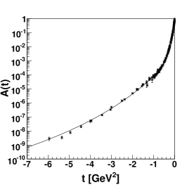
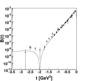
Figure 5.3: Behavior of the deuteron elastic structure functions $A(t)$ and $B(t)$ obtained by a simultaneous comparison of our $U\&A$ model of the deuteron EM structure to existing experimental data on $A(t)$, $B(t)$ and polarization observable $t_{20}$

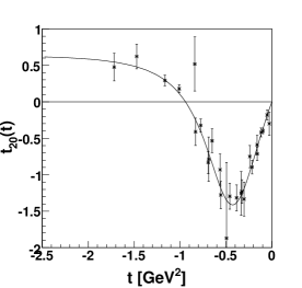
Figure 5.4: Behavior of the deuteron tensor polarization observable ${t}_{20}(t)$ obtained by a simultaneous comparison of our $U\&A$ model of the deuteron EM structure to existing experimental data on $A(t)$, $B(t)$ and $t_{20}$

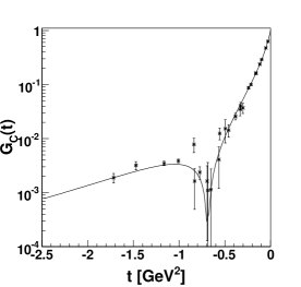
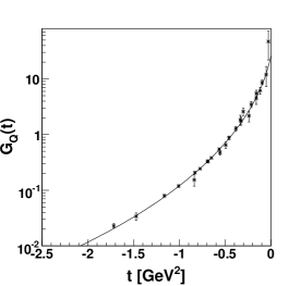
Figure 5.5: The predicted behavior of the space-like deuteron charge form factor $G_{C}(t)$ and quadrupole form factor $G_{Q}(t)$ by our U&A model of the deuteron electromagnetic structure and their comparison to existing experimental data.

on the effective thresholds $t_{inC},t_{inM},t_{inQ}$ and on unknown ratios $a_{C:x}$ and $a_{Q:x}$.

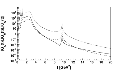
Figure 5.6: The predicted time-like behavior of the absolute values of the deuteron complex EM form factors $G_{C}(t),G_{M}(t),G_{Q}(t)$ by our U&A model of the deuteron electromagnetic structure. Full line corresponds to the charge FF $|G_{C}(t)|$, dashed line corresponds to the magnetic FF $|G_{M}(t)|$ and dotted line corresponds to the quadrupole FF $|G_{Q}(t)|$.

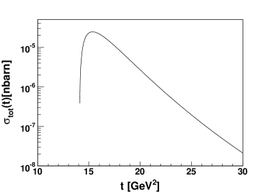
Figure 5.7: The total cross section behavior of the $e^{-}e^{+}\rightarrow d\bar{d}$ annihilation process to be estimated by our U&A model of the deuteron EM structure.

Naturally, we can fix masses $m_{v}$ and widths $\Gamma_{v}$ of all known vector mesons ($\omega,\phi,\omega^{\prime},\omega^{\prime\prime},\phi^{\prime},$ $J/\Psi$), what means, that there will remain seven free parameters, which are numerically evaluated in the optimal description of all available experimental data on the deuteron elastic structure functions $A(t)$, $B(t)$ and the polarization observable ${t}_{20}(t)$. The results were obtained by using CERN program ROOT [144] and corresponding behaviors are shown on Figs. 5.3, 5.4 and 5.5, together with data. The values of free parameters are given in Table 5.1.

Table 5.1: Fitted parameters of the U&A model of the deuteron EM structure.

${m_{x}}{\mathrm{MeV}}$$1^{1^{1}}$	${\Gamma_{x}}{\mathrm{MeV}}$	${t_{inC}}{\mathrm{GeV}^{2}}$	${t_{inM}}{\mathrm{GeV}^{2}}$	${t_{inQ}}{\mathrm{GeV}^{2}}$	$a_{C:x}$	$a_{Q:x}$
$504.9\pm 0.1$	$677.6\pm 0.2$	$18.2\pm 0.1$	$20.2\pm 0.2$	$7.8\pm 0.1$	$3.43\pm 0.01$	$28.14\pm 0.03$

As one can see, we have obtained a quite reasonable description of the deuteron structure functions $A(t)$, $B(t)$ and polarization observable ${t}_{20}(t)$, however with $\chi^{2}/n.d.f.=4.61$ indicating an inconsistency among independent sets of data.

Moreover, the constructed model with the same values of free parameters can be used for the description of experimental data on the additional deuteron EM FFs $G_{Cd}(t)$ and $G_{Qd}(t)$, as well as for estimation of all three deuteron EM FFs time-like region behavior ( see Fig. 5.6). They allow us to estimate the total cross section of the electron-positron annihilation into deuteron-antideuteron (5.2), which is planned to be measured on BES3 in Peking for the first time.

Its predicted behavior is given in Fig. 5.7.

5.3 Study of two-photon contribution relevance into deuteron electromagnetic structure by impulse approximation

As a result of a consideration of one-photon exchange approximation in elastic scattering of electrons on any hadron with nonzero spin, one obtains the same expression in the form for the differential cross-section in the laboratory system to be expressed through the elastic structure functions $A(t)$ and $B(t)$. For comparison see (2.17) and (2.21).

If also two-photon contributions are considered, no more simple form of the differential cross-section of elastic scattering of electrons on hadrons with nonzero spin is obtained.

In the previous chapter we have analysed the new JLab proton polarization data [101, 102, 103] in the framework of the ten-resonance $U\&A$ model [97] of nucleon EM structure. The parameters, in comparison with those in [97] have been found to be changed very little. But a reasonable description of the new JLab data was achieved, whereby almost nothing has been changed in the description of $G_{Mp}(t)$, $G_{En}(t)$, $G_{Mn}(t)$ in both the space-like and time-like regions and $|G_{Ep}(t)|$ in the time-like region. However, the existence of the zero (see the full line in Fig. 4.3), i.e. a diffraction minimum in the space-like region of $|G_{Ep}(t)|$ at $t=-Q^{2}\approx-13\leavevmode\nobreak\ GeV^{2}$ is predicted by such ten-resonance unitary and analytic model and so, $|G_{Ep}(t)|$ has no more dipole behavior in the space-like region.

Recently it was suggested [145]-[147] that the two-photon corrections could be responsible for the found non-dipole behavior of $|G_{Ep}(t)|$ in the space-like region. Then there is a natural question arisen, if two-photon corrections play so important role in the elastic electron-proton scattering, what about a size of two-photon corrections in elastic electron-deuteron scattering.

In this paragraph [148] the non-relativistic impulse approximation (NIA), which requires a knowledge only of the deuteron wave functions and the nucleon EM FFs, is used to study the previous question.

As deuteron can be found in S- ($\approx 96\%$) and D-state ($\approx 4\%$), then NN non-relativistic full wave function of the deuteron can be written in terms of two scalar wave functions

$$\Psi_{abm} = \sum_{l}\sum_{m_{s}}\frac{z_{l}(r)}{r}Y_{l,m-m_{s}}(\widehat{\mathbf{r}})\chi_{ab}^{1m_{s}}$$

$$\left\langle l,1,m-m_{s},m_{s}|1,m\right\rangle$$

$$= \frac{u(r)}{r}Y_{0,0}(\widehat{\mathbf{r}})\chi_{ab}^{1m}+$$

$$+ \frac{w(r)}{r}\sum_{m_{s}}Y_{2,m-m_{s}}(\widehat{\mathbf{r}})\chi_{ab}^{1m_{s}}\left\langle 2,1,m-m_{s},m_{s}|1,m\right\rangle,$$

where $\left\langle l,1,m-m_{s},m_{s}|1,m\right\rangle$ are Clebsh-Gordan coefficients, $Y_{l,m_{l}}$ are spherical harmonics normalized to unity on the unit sphere, $\chi_{ab}^{1m_{s}}$ is the spin part of the wave function and $z_{0}=u$, $z_{2}=w$ are reduced $S-$ and $D$-state wave functions, respectively.

The normalization condition

$$\int d^{3}r\Psi_{abm^{\prime}}^{{\dagger}}\Psi_{abm}=\delta_{m^{\prime}m}$$

implies normalization

$$\int_{0}^{\infty}dr\left[u^{2}(r)+w^{2}(r)\right]=1,$$ (5.15)

which could be understood as the probability of finding deuteron in $S-$ or $D$-state. The $D$-state probability

$$P_{D}=\int_{0}^{\infty}drw^{2}(r)$$

is an interesting measurement of the strength of the tensor component of the $NN$ force.

The non-relativistic wave functions are calculated from the Schrödinger equation using potentials adjusted to fit NN scattering data for laboratory energies from 0 to 350 MeV. In this paper we will use one of the most common potentials called Paris potential [149], which depends on the minimal number of free parameters and it was among the first potentials to be determined from such realistic fit. The $S-$ and $D-$state wave functions determined from this model are presented in Fig. 5.8.

The deuteron is a pure iso-scalar target, therefore within NIA its FFs depend only on the iso-scalar nucleon form factors $G_{EN}^{s}$ and $G_{MN}^{s}$

$$G_{EN}^{s} = G_{Ep}+G_{En}$$

$$G_{MN}^{s} = G_{Mp}+G_{Mn}$$ (5.16)

in the following way

$$G_{Cd} = G_{EN}^{s}D_{C}$$

$$G_{Md} = \frac{m_{d}}{2m_{p}}\left[G_{MN}^{s}D_{M}+G_{EN}^{s}D_{E}\right]$$ (5.17)

$$G_{Qd} = G_{EN}^{s}D_{Q},$$

Figure 5.8: The $S$ and $D$ state deuteron wave functions ($u$,$w$) behaviors for Paris potential [149].

where the body form factors $D_{C}$, $D_{M}$, $D_{E}$ and $D_{Q}$ are functions of the momentum transfer squared $t$. The non-relativistic formulas for the body form factors $D$ involve overlaps of the wave functions $u(r),w(r)$, weighted by spherical Bessel functions

$$D_{C}(q^{2}) = \int_{0}^{\infty}dr\left[u^{2}(r)+w^{2}(r)\right]j_{0}(\kappa)$$

$$D_{M}(q^{2}) = \int_{0}^{\infty}dr\left[2u^{2}(r)-w^{2}(r)\right]j_{0}(\kappa)+$$

$$+ \left[\sqrt{2}u(r)w(r)+w^{2}(r)\right]j_{2}(\kappa)$$

$$D_{E}(q^{2}) = \frac{3}{2}\int_{0}^{\infty}drw^{2}(r)\left[j_{0}(\kappa)+j_{2}(\kappa)\right]$$

$$D_{Q}(q^{2}) = \frac{3}{\sqrt{2}\eta}\int_{0}^{\infty}drw(r)\left[u(r)-\frac{w(r)}{\sqrt{8}}\right]j_{2}(\kappa),$$

where $\kappa=qr/2$. At $q^{2}=0,$ the body form factors become

$$D_{C}(0) = \int_{0}^{\infty}dr\left[u^{2}(r)+w^{2}(r)\right]=1$$

$$D_{M}(0) = \int_{0}^{\infty}dr\left[2u^{2}(r)-w^{2}(r)\right]=2-3P_{D}$$

$$D_{E}(0) = \frac{3}{2}\int_{0}^{\infty}drw^{2}(r)=\frac{3}{2}P_{D}$$ (5.19)

$$D_{Q}(0) = \frac{m_{d}^{2}}{\sqrt{50}}\int_{0}^{\infty}drw(r)\left[u(r)-\frac{w(r)}{\sqrt{8}}\right]$$

giving the non-relativistic predictions

$$Q_{d} = D_{Q}(0)$$ (5.20)

$$\mu_{d} = \mu_{N}^{s}D_{M}(0)+D_{E}(0)=\mu_{N}^{s}(2-3P_{D})+1.5P_{D},$$

where $Q_{d}$ is the quadrupole moment of the deuteron, $\mu_{d}$ is the magnetic moment of the deuteron and $\mu_{N}^{s}=\frac{1}{2}(\mu_{p}+\mu_{n}-1)$ is the isoscalar nucleon magnetic moment. The experimental value of the deuteron magnetic moment $\mu_{d}=1.7139$, leads to the probability of $D$-state $P_{D}=4.0\%.$ But this is only approximate value, because the magnetic moment is very sensitive to relativistic corrections.

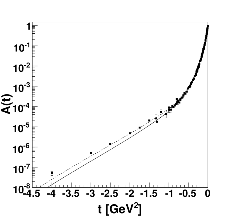
Figure 5.9: Deuteron structure function $A(t)$ data and their comparison with NIA predictions using non-dipole (full line) and dipole (dashed line) $G_{Ep}(t)$ behavior.

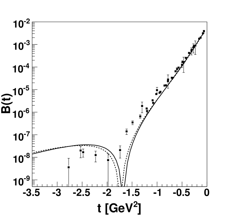
Figure 5.10: Deuteron structure function $B(t)$ data and their comparison with NIA predictions using non-dipole (full line) and dipole (dashed line) $G_{Ep}(t)$ behavior.

Experimentally the EM structure of the deuteron is measured in the elastic scattering of electrons on deuterons, described by the differential cross-section (2.21) to be calculated in the one-photon-exchange approximation with the deuteron elastic structure functions. In order to see predicted behaviors of the deuteron elastic structure functions $A(t)$ and $B(t)$ to be caused by the non-dipole behavior of the proton electric FF with the zero around $t=-Q^{2}=-13GeV^{2}$, we use the $G_{Ep}(t)$ (see full line in Fig. 4.3) together with all other nucleon FF behaviors in the calculation of the nucleon EM FF isoscalar parts by means of the relation (5.16). Then through the relations (2.22) and (5.17) one comes to the behavior of $A(t)$ and $B(t)$ as presented in Fig. 5.9 and Fig. 5.10, respectively, by full lines.

For comparison the deuteron elastic structure functions $A(t),B(t)$ are predicted also by means of the nucleon EM FFs [97] obtained in the elastic scattering of unpolarized electrons on unpolarized protons by Rosenbluth technique, i.e. by using the proton electric FF in $t<0$ region having more or less dipole behavior (see dashed line in Fig. 4.3). The results are presented in Fig. 5.9 and Fig. 5.10 by dashed lines. As one can see from figures the examined difference is negligible, indicating that the two-photon-exchange contribution is unimportant for the unpolarized electron-deuteron elastic scattering in comparison with the unpolarized electron-proton elastic scattering.

6 Sea-strange quark contributions to electromagnetic structure of hadrons

Hadrons are classified according to the $SU(3)$ symmetries into multiplets, the most of them are known nonet of pseudoscalar mesons and $1/2^{+}$ octet of baryons to be already treated in this review. The mesons in the quark model are $q\bar{q}$ bound states and members of octuplet are 3-quark $qqq$ configurations plus any number of quark-antiquark pairs of light quarks u, d and s.

At the nonet of pseudoscalar mesons the $\pi$ and $\eta$ are compound from only up and down quarks, whereas $K$-mesons and $\eta^{\prime}$ to some extent are compound also from strange quark.

At the octet of baryons only proton and nucleon are compound from up and down quarks. The hyperons contain one or two strange quarks.

This section we start with experimental indications on sea $s\bar{s}$ pairs contributions to the nucleon structure.

They are as follows

• Pion-nucleon sigma term $\sigma_{\pi N}$

  The $\sigma$-term of $\pi N$ scattering is defined by the relation

  $$\sigma_{\pi N}(t=0)=\langle p|(\bar{u}u+\bar{d}d)|p\rangle$$ (6.1)

  and it can be determined from extrapolation of scattering data on the isospin even $\pi N$ on shell amplitude $\Sigma=f_{\pi}^{2}\bar{D}(\nu,t)$ to the unphysical Cheng-Dashen point $\nu=0$, $t=2\mu^{2}$ in the chiral limit $m_{\pi}=m_{u}=m_{d}=0$.

  The results obtained from the analysis of $\pi N$ data are now

  $$\Sigma(2\mu^{2})=\sigma_{\pi N}(2\mu^{2})=60MeV$$ (6.2)

  and consequently $\sigma_{\pi N}(0)=45MeV$.

  On the other hand, the SU(3) mass splittings are due to the quark mass term $H_{m}$ (the isospin symmetry is assumed) in the QCD Hamiltonian

  $$H_{m}=\hat{m}(\bar{u}u+\bar{d}d)+m_{s}\bar{s}s$$ (6.3)

  in which $m_{s}$ is the strange quark mass. The latter can be written in terms of singlet and octet contributions:

  $$H_{m}=1/3(m_{s}+2\hat{m})(\bar{u}u+\bar{d}d+\bar{s}s)-1/3(m_{s}-\hat{m})((\bar{u}u+\bar{d}d-2\bar{s}s).$$ (6.4)

  The octet matrix element

  $$\delta=\langle N|(\bar{u}u+\bar{d}d-2\bar{s}s)|N\rangle=\langle N|(\bar{u}u+\bar{d}d)|N\rangle-2\langle N|\bar{s}s|N\rangle$$ (6.5)

  is determined from the octet masses by current algebra and SU(3) symmetry. As a result one finds

  $$\delta\simeq 26MeV$$ (6.6)

  Since $\sigma_{\pi N}\neq\delta$, the scalar strange quark density $\langle N|\bar{s}s|N\rangle$ is non-vanishing, leading to the following fraction of strange quarks in the proton

  $$Y=\frac{\langle N|\bar{s}s|N\rangle}{\langle N|\bar{u}u+\bar{d}d|N\rangle}=0.21$$ (6.7)

• Proton spin crisis

  Deep inelastic scattering of polarized charged leptons ($e^{-}$ or $\mu^{-}$) by polarized protons has been investigated at CERN and SLAC and it was found so-called EMC effect, i.e. quarks appeared to contribute very little to the proton spin.

  If $\triangle\Sigma$ is the fraction of proton spin contributed by light quarks, then

  $$\triangle\Sigma=\triangle u+\triangle d+\triangle s,$$ (6.8)

  where $\triangle q^{\prime}s$ are integrals

  $$\triangle q\equiv\int_{0}^{1}dx\{[q^{\uparrow}(x)-\bar{q}^{\uparrow}(x)]-[q^{\downarrow}(x)-\bar{q}^{\downarrow}(x)]\}$$ (6.9)

  of the difference of differences between parallel and antiparallel probability quark distributions, $q^{\uparrow\downarrow}(x)$ and $\bar{q}^{\uparrow\downarrow}(x)$ (q=u,d,s), for quarks and antiquarks with spin parallel and antiparallel to the proton spin and $x$ is the Bjorken scaling variable.

  In the non-relativistic constituent quark model

  $$\triangle u=4/3,\quad\quad\quad\triangle d=-1/3,\quad\quad\quad\triangle s=0$$ (6.10)

  and

  $$\triangle\Sigma=1.$$ (6.11)

  However, the $\triangle u$, $\triangle d$ and $\triangle s$ can be determined from DIS spin-dependent proton structure function $g_{1}^{p}(x)$ and baryon $\beta$-decays.

  Really

  1. The integral of $g_{1}^{p}(x)$ is a sum over $\triangle q^{\prime}s$, each weighted by the square of that flavor quark’s electric charge

     $$\Gamma_{1}^{p}\equiv\int g_{1}^{p}(x)dx=1/2\{4/9\triangle u+1/9\triangle d+1/9\triangle s\};$$ (6.12)

  2. The matrix elements $F$ and $D$ measured in hyperon decays are related to $\triangle u$ - $\triangle d$ and $\triangle u$ + $\triangle d$ - 2$\triangle s$ as follows

     $$g_{A}\equiv F+D =\triangle u-\triangle d$$ (6.13)

     $$3F-D =\triangle u+\triangle d-2\triangle s.$$ (6.14)

     A recent analysis of $\Gamma_{1}^{p}$, $F$ and $D$ finds

     $$\triangle u=0.83\pm 0.03;\quad\quad\quad\triangle d=-0.43\pm 0.03;\quad\quad\quad\triangle s=-0.10\pm 0.03$$ (6.15)

     and

     $$\triangle\Sigma=0.30\pm 0.05$$ (6.16)

     indicating that very little of the proton spin is carried by the light quarks and that the strange sea is polarized antiparallel to the proton spin.

• OZI rule violation. The OZI rule states that quark diagrams with disconnected quark lines are strongly suppressed. As a result the process $\bar{p}p\to\phi X$ has to be remarkably suppressed in comparison with the process $\bar{p}p\to\omega X$.

  Recent experiments at LEAR at CERN have found violations of the OZI rule of up to two orders of the magnitude in $\bar{p}N\to\phi X$ annihilations.

  Such data could be explained if there are $\bar{s}s$ pairs present in the nucleon (and antinucleon).

• Neutrino experiments

  Elastic $\nu$ and $\bar{\nu}$ scattering on protons is sensitive to strange axial-vector form factor, indicating on the presence of $\bar{s}s$ pairs in the proton.

  On the other hand, in deep inelastic scattering of $\nu$ and $\bar{\nu}$ on protons the charmed particles can be produced in $d\to c$ and $s\to c$ transitions. The probability

  $$d\to c \sim \sin^{2}{\theta_{c}}$$

  $$s\to c \sim \cos^{2}{\theta_{c}}$$

  where $\theta_{c}$=0.23 is the Cabibbo angle.

  Due to the smallness of $\theta_{c}$ the $s\to c$ transition is dominant and gives the probability of studying the strange sea in $N$.

All these evidences for strangeness in $N$ mean that various elements of

• scalar $\bar{s}s$

• pseudoscalar $\bar{s}\gamma_{5}s$

• vector $\bar{s}\gamma_{\mu}s$

• axial-vector $\bar{s}\gamma_{\mu}\gamma_{5}s$

• tensor $\bar{s}\sigma_{\mu\nu}s$

currents, appearing in various processes with nucleons $N$, are non vanishing and it has sense to investigate them theoretically.

Further we concentrate [150] only to the nucleon matrix element of the strange-quark vector current $J^{s}_{\mu}=\bar{s}\gamma_{\mu}s$, which is experimentally accessible in parity-violating elastic and quasi-elastic electron scattering from the proton and light atomic nuclei, where the strange electric and the strange magnetic nucleon form factors (FFs) (or their combinations) are measured.

6.1 Prediction of strange nucleon form factors behaviors

The momentum dependence of the nucleon matrix element of the strange-quark vector current $J^{s}_{\mu}$=$\bar{s}\gamma_{\mu}s$ is contained in the strange Dirac $F^{s}_{1}(t)$ and Pauli $F^{s}_{2}(t)$ nucleon FFs

$$\langle N|\bar{s}\gamma_{\mu}s|N\rangle=\bar{u}(p^{{}^{\prime}})\left[\gamma_{\mu}F^{s}_{1}(t)+i{{\sigma_{\mu\nu}q^{\nu}}\over{2m_{N}}}F^{s}_{2}(t)\right]u(p),$$ (6.17)

by means of which the strange electric and strange magnetic nucleon FFs are defined

$$G_{E}^{s}(t)=F_{1}^{s}(t)+\frac{t}{4m_{N}^{2}}F_{2}^{s}(t),\quad G_{M}^{s}(t)=F_{1}^{s}(t)+F_{2}^{s}(t).$$ (6.18)

The latter can be measured in parity-violating elastic and quasi-elastic scattering of electrons on protons and light atomic nuclei.

Since the strange-quark vector current $J_{\mu}^{s}=\bar{s}\gamma_{\mu}s$ carries the quantum numbers of the isoscalar part of the EM current $J_{\mu}^{I=0}$ and thus both currents couple to the nucleon through the same intermediate states, it is natural to expect [151] that one can extract the behavior of strange Dirac and Pauli nucleon FFs just from the isoscalar parts of Dirac and Pauli nucleon EM FFs.

The main idea of a prediction of strange nucleon FFs behaviors from the known isoscalar parts of the Dirac and Pauli nucleon EM FFs is based on two assumptions

• the $\omega-\phi$ mixing is valid also for coupling constants between EM current (the strong strange quark current as well) and vector-meson

  $$\frac{1}{f_{\omega}}=\frac{1}{f_{\omega_{0}}}\cos{\epsilon}-\frac{1}{f_{\phi_{0}}}\sin{\epsilon};\quad\frac{1}{f_{\phi}}=\frac{1}{f_{\omega_{0}}}\sin{\epsilon}+\frac{1}{f_{\phi_{0}}}\cos{\epsilon},$$ (6.19)

  where $\epsilon=3.7^{\circ}$ is a deviation from the ideally mixing angle $\theta_{0}=35.3^{\circ}$;

• the quark current of some flavor couples with universal strength $\kappa$ exclusively to the vector-meson wave function component of the same flavor

  $$\langle 0|\bar{q}_{r}\gamma q_{r}|(\bar{q}_{t}q_{t})_{V}\rangle=\kappa m^{2}_{V}\delta_{rt}\varepsilon_{\mu},$$ (6.20)

where $m_{V}$ and $\varepsilon_{\mu}$ are the mass and the polarization vector of the considered vector-meson.

Starting from a definition of the virtual-photon vector-meson transition coupling constants $1/f^{e}_{V}$ by the relation

$$<0|J^{e}_{\mu}|V>=\frac{m_{V}^{2}}{f^{e}_{V}}\epsilon_{\mu}$$ (6.21)

and the second assumption for the isoscalar EM current $J^{I=0}_{\mu}$ to be expressed by quark fields, one comes to the equations

$$<0|J^{I=0}_{\mu}|\omega_{0}> = <0|\frac{1}{6}(\bar{u}\gamma_{\mu}u+\bar{d}\gamma_{\mu}d)-\frac{1}{3}\bar{s}\gamma_{\mu}s|\frac{1}{\sqrt{2}}(|\bar{u}u>+|\bar{d}d>)=$$ (6.22)

$$= \frac{1}{6}(\frac{1}{\sqrt{2}}+\frac{1}{\sqrt{2}})\kappa m^{2}_{\omega_{0}}\varepsilon_{\mu}\equiv\frac{m^{2}_{\omega_{0}}}{f^{e}_{\omega_{0}}}\varepsilon_{\mu}$$

$$<0|J^{I=0}_{\mu}|\phi_{0}> = <0|\frac{1}{6}(\bar{u}\gamma_{\mu}u+\bar{d}\gamma_{\mu}d)-\frac{1}{3}\bar{s}\gamma_{\mu}s|\bar{s}s>)=$$ (6.23)

$$= -\frac{1}{3}\kappa m^{2}_{\phi_{0}}\varepsilon_{\mu}\equiv\frac{m^{2}_{\phi_{0}}}{f^{e}_{\phi_{0}}}\varepsilon_{\mu}$$

from where expressions for EM coupling constants follow

$$\frac{1}{f^{e}_{\omega_{0}}}=\frac{1}{6}(\frac{1}{\sqrt{2}}+\frac{1}{\sqrt{2}})\kappa=\frac{1}{\sqrt{6}}\frac{1}{\sqrt{3}}\kappa;\quad\frac{1}{f^{e}_{\phi_{0}}}=-\frac{1}{3}\kappa=-\frac{1}{\sqrt{6}}\sqrt{\frac{2}{3}}\kappa.$$ (6.24)

Substituting the latter into the first assumption, together with identities $\frac{1}{\sqrt{3}}=\sin{\theta_{0}}$ and $\sqrt{\frac{2}{3}}=\cos{\theta_{0}}$, one obtains coupling constants of real $\omega$ and $\phi$

$$\frac{1}{f^{e}_{\omega}}=\frac{\kappa}{\sqrt{6}}\sin(\varepsilon+\theta_{0};\quad\frac{1}{f^{e}_{\phi}}=-\frac{\kappa}{\sqrt{6}}\cos(\varepsilon+\theta_{0}).$$ (6.25)

These relations, together with $\frac{1}{f^{e}_{\rho}}=\frac{1}{\sqrt{2}}\kappa$ following from

$$<0|J^{I=1}_{\mu}|\rho> = <0|\frac{1}{2}(\bar{u}\gamma_{\mu}u-\bar{d}\gamma_{\mu}d)|\frac{1}{\sqrt{2}}(|\bar{u}u>-|\bar{d}d>)=$$ (6.26)

$$= \frac{1}{2}(\frac{1}{\sqrt{2}}+\frac{1}{\sqrt{2}})\kappa m^{2}_{\rho}\varepsilon_{\mu}\equiv\frac{m^{2}_{\rho}}{f^{e}_{\rho}}\varepsilon_{\mu},$$

give for the ratios of the universal vector-meson coupling constants the values

$\frac{1}{f^{e}_{\rho}}:\frac{1}{f^{e}_{\omega}}:\frac{1}{f^{e}_{\phi}}=0.71:0.25:(-0.32)$

in a very good agreement with experimental values

$\frac{1}{f^{e}_{\rho}}:\frac{1}{f^{e}_{\omega}}:\frac{1}{f^{e}_{\phi}}=0.79:0.23:(-0.31)$

obtained from leptonic widths $\Gamma(V\to e^{+}e^{-})$ of considered vector-mesons. Just this agreement demonstrates the previous two assumptions to be compatible with physical reality and one can extend their validity also for strong strange-quark current vector-meson transition coupling constants $1/f^{s}_{V}$.

Then analogically one can write for the strong strange-quark current the equations

$$<0|J^{s}_{\mu}|\omega_{0}>=<0|(\bar{s}\gamma_{\mu}s|\frac{1}{\sqrt{2}}(|\bar{u}u>+|\bar{d}d>)=0\equiv\frac{m^{2}_{\omega_{0}}}{f^{s}_{\omega_{0}}}\varepsilon_{\mu}$$ (6.27)

$$<0|J^{s}_{\mu}|\phi_{0}>=<0|(\bar{s}\gamma_{\mu}s||\bar{s}s>=1.\kappa m^{2}_{\phi_{0}}\varepsilon_{\mu}\equiv\frac{m^{2}_{\phi_{0}}}{f^{s}_{\phi_{0}}}\varepsilon_{\mu},$$ (6.28)

from where one gets $\frac{1}{f^{s}_{\omega_{0}}}=0$ and $\frac{1}{f^{s}_{\phi_{0}}}=1.\kappa$. Substituting them into $\omega-\phi$ mixing relations one comes to the strange coupling constants of the real $\omega$ and $\phi$

$$\frac{1}{f^{s}_{\omega}}=-\kappa\sin{\varepsilon};\quad\frac{1}{f^{s}_{\phi}}=+\kappa\cos{\varepsilon}$$ (6.29)

Bringing these expressions for $\omega$ and $\phi$ vector mesons into ratios with EM coupling constants (6.25), respectively, one gets rid of the unknown parameter $\kappa$ and comes to the relations

$$({f^{(i)}_{\omega NN}}/{f^{s}_{\omega}}) = -\sqrt{6}\frac{\sin{\epsilon}}{\sin(\epsilon+\theta_{0})}({f^{(i)}_{\omega NN}}/{f^{e}_{\omega}})$$

$$({f^{(i)}_{\phi NN}}/{f^{s}_{\phi}}) = -\sqrt{6}\frac{\cos{\epsilon}}{\cos(\epsilon+\theta_{0})}({f^{(i)}_{\phi NN}}/{f^{e}_{\phi}})\quad(i=1,2)$$ (6.30)

giving a possibility to calculate the unknown strange coupling constant ratios (parameters of strange nucleon FFs) from the known EM coupling constant ratios (parameters of EM nucleon FFs) to be determined in a description of all existing nucleon EM FF data by a suitable model of the EM structure of nucleons.

The derived relations (6.30) are valid also for any pairs of excited states $\omega^{\prime}$,$\phi^{\prime}$, $\omega^{\prime\prime}$, $\phi^{\prime\prime}$, etc. of the ground state of $\omega$ and $\phi$ isoscalar vector-mesons.

Then for a prediction of strange nucleon form factors the $U\&A$ model of the nucleon EM structure [97] will be used, which comprises all known nucleon FF properties to be contained in the following models of isoscalar parts of Dirac and Pauli nucleon EM FFs

$$F^{I=0}_{1}[V(t)] = \left(\frac{1-V^{2}}{1-V^{2}_{N}}\right)^{4}\bigg{\{}\frac{1}{2}L(V_{\omega^{\prime\prime}})L(V_{\omega^{\prime}})+[L(V_{\omega^{\prime\prime}})L(V_{\omega})\frac{(C_{\omega^{\prime\prime}}-C_{\omega})}{(C_{\omega^{\prime\prime}}-C_{\omega^{\prime}})}-$$ (6.31)

$$- L(V_{\omega^{\prime}})L(V_{\omega})\frac{(C_{\omega^{\prime}}-C_{\omega})}{(C_{\omega^{\prime\prime}}-C_{\omega^{\prime}})}-L(V_{\omega^{\prime\prime}})L(V_{\omega^{\prime}})](f^{(1)}_{\omega NN}/f^{e}_{\omega})+$$

$$+ [L(V_{\omega^{\prime\prime}})L(V_{\phi})\frac{(C_{\omega^{\prime\prime}}-C_{\phi})}{(C_{\omega^{\prime\prime}}-C_{\omega^{\prime}})}-L(V_{\omega^{\prime}})L(V_{\phi})\frac{(C_{\omega^{\prime}}-C_{\phi})}{(C_{\omega^{\prime\prime}}-C_{\omega^{\prime}})}-$$

$$- L(V_{\omega^{\prime\prime}})L(V_{\omega^{\prime}})](f^{(1)}_{\phi NN}/f^{e}_{\phi})\bigg{\}}$$

$$F^{I=0}_{2}[V(t)] = \left(\frac{1-V^{2}}{1-V^{2}_{N}}\right)^{6}\bigg{\{}L(V_{\omega^{\prime\prime}})L(V_{\omega^{\prime}})L(V_{\omega})\left[1-{\frac{C_{\omega}}{(C_{\omega^{\prime\prime}}-C_{\omega^{\prime}})}}\right.\times$$ (6.32)

$$\times \left.\left(\frac{(C_{\omega^{\prime\prime}}-C_{\omega})}{C_{\omega^{\prime}}}-\frac{(C_{\omega^{\prime}}-C_{\omega})}{C_{\omega^{\prime\prime}}}\right)\right](f^{(2)}_{\omega NN}/f^{e}_{\omega})+$$

$$+ L(V_{\omega^{\prime\prime}})L(V_{\omega^{\prime}})L(V_{\phi})\left[1-{\frac{C_{\phi}}{(C_{\omega^{\prime\prime}}-C_{\omega^{\prime}})}}\left(\frac{(C_{\omega^{\prime\prime}}-C_{\phi})}{C_{\omega^{\prime}}}\right.\right.-$$

$$- \left.\left.\left.\frac{(C_{\omega^{\prime}}-C_{\phi})}{C_{\omega^{\prime\prime}}}\right)\right](f^{(2)}_{\phi NN}/f^{e}_{\phi})\right\}$$

and of the Dirac and Pauli strange nucleon FFs

$$F^{s}_{1}[V(t)] = \left(\frac{1-V^{2}}{1-V^{2}_{N}}\right)^{4}\bigg{\{}\left[L(V_{\omega^{\prime\prime}})L(V_{\omega})\frac{(C_{\omega^{\prime\prime}}-C_{\omega})}{(C_{\omega^{\prime\prime}}-C_{\omega^{\prime}})}\right.-$$ (6.33)

$$- \left.L(V_{\omega^{\prime}})L(V_{\omega})\frac{(C_{\omega^{\prime}}-C_{\omega})}{(C_{\omega^{\prime\prime}}-C_{\omega^{\prime}})}-L(V_{\omega^{\prime\prime}})L(V_{\omega^{\prime}})\right](f^{(1)}_{\omega NN}/f^{s}_{\omega})+$$

$$+ \bigg{[}L(V_{\omega^{\prime\prime}})L(V_{\phi})\frac{(C_{\omega^{\prime\prime}}-C_{\phi})}{(C_{\omega^{\prime\prime}}-C_{\omega^{\prime}})}-L(V_{\omega^{\prime}})L(V_{\phi})\frac{(C_{\omega^{\prime}}-C_{\phi})}{(C_{\omega^{\prime\prime}}-C_{\omega^{\prime}})}-$$

$$- L(V_{\omega^{\prime\prime}})L(V_{\omega^{\prime}})\bigg{]}(f^{(1)}_{\phi NN}/f^{s}_{\phi})\bigg{\}}$$

$$F^{s}_{2}[V(t)] = \left(\frac{1-V^{2}}{1-V^{2}_{N}}\right)^{6}\bigg{\{}L(V_{\omega^{\prime\prime}})L(V_{\omega^{\prime}})L(V_{\omega})\bigg{[}1-{\frac{C_{\omega}}{(C_{\omega^{\prime\prime}}-C_{\omega^{\prime}})}}\times$$

$$\times \left(\frac{(C_{\omega^{\prime\prime}}-C_{\omega})}{C_{\omega^{\prime}}}-\frac{(C_{\omega^{\prime}}-C_{\omega})}{C_{\omega^{\prime\prime}}}\right)\bigg{]}(f^{(2)}_{\omega NN}/f^{s}_{\omega})+L(V_{\omega^{\prime\prime}})L(V_{\omega^{\prime}})L(V_{\phi})\times$$

$$\times \left[1-\frac{C_{\phi}}{(C_{\omega^{\prime\prime}}-C_{\omega^{\prime}})}\left(\frac{(C_{\omega^{\prime\prime}}-C_{\phi})}{C_{\omega^{\prime}}}-\frac{(C_{\omega^{\prime}}-C_{\phi})}{C_{\omega^{\prime\prime}}}\right)\right](f^{(2)}_{\phi NN}/f^{s}_{\phi})\bigg{\}},$$

where

$$L(V_{r})=\frac{(V_{N}-V_{r})(V_{N}-V^{\ast}_{r})(V_{N}-1/V_{r})(V_{N}-1/V^{\ast}_{r})}{(V-V_{r})(V-V^{\ast}_{r})(V-1/V_{r})(V-1/V^{\ast}_{r})},$$

$$C_{r}=\frac{(V_{N}-V_{r})(V_{N}-V^{\ast}_{r})(V_{N}-1/V_{r})(V_{N}-1/V^{\ast}_{r})}{-(V_{r}-1/V_{r})(V^{\ast}_{r}-1/V^{\ast}_{r})},$$

$$V_{N}=V(t)_{|t=0};V_{r}=V(t)_{|t=(m_{r}-i\Gamma_{r}/2)^{2}};(r=\omega,\phi,\omega^{\prime},\omega^{\prime\prime}),$$

$$V(t)=i\frac{\sqrt{[\frac{t_{N\bar{N}}-t^{I=0}_{0}}{t^{I=0}_{0}}]^{1/2}+[\frac{t-t^{I=0}_{0}}{t^{I=0}_{0}}]^{1/2}}-\sqrt{[\frac{t_{N\bar{N}}-t^{I=0}_{0}}{t^{I=0}_{0}}]^{1/2}-[\frac{t-t^{I=0}_{0}}{t^{I=0}_{0}}]^{1/2}}}{\sqrt{[\frac{t_{N\bar{N}}-t^{I=0}_{0}}{t^{I=0}_{0}}]^{1/2}+[\frac{t-t^{I=0}_{0}}{t^{I=0}_{0}}]^{1/2}}+\sqrt{[\frac{t_{N\bar{N}}-t^{I=0}_{0}}{t^{I=0}_{0}}]^{1/2}-[\frac{t-t^{I=0}_{0}}{t^{I=0}_{0}}]^{1/2}}}$$ (6.35)

and $t_{N\bar{N}}=4m_{N}^{2}$ is a square-root branch point corresponding to $N\bar{N}$ threshold.

Figure 6.1: Predicted strange electric and magnetic nucleon FFs behaviors

Figure 6.2: Predicted behaviors of the strange nucleon FFs in the time-like region

The expressions (6.31) and (6.32) for $F_{1}^{I=0},F_{2}^{I=0}$, respectively, together with similar expressions for $F_{1}^{I=1},F_{2}^{I=1}$ [97] were used for a description of all solid nucleon EM FF data and a reasonable description of them has been achieved. The found numerical values of $(f^{(i)}_{\omega NN}/f^{e}_{\omega})$, $(f^{(i)}_{\phi NN}/f^{e}_{\phi})\quad i=1,2$ in the relations (6.31), (6.32) are used to calculate the unknown strange coupling constant ratios $(f^{(i)}_{\omega NN}/f^{s}_{\omega}),(f^{(i)}_{\phi NN}/f^{s}_{\phi})\quad i=1,2$ in (6.33), (6.1) by means of the relations (6.30). As a result the behaviors of the strange nucleon FFs are predicted (see Fig. 6.1) without the use of any experimental point obtained in parity-violating elastic and quasi-elastic scattering of electrons on protons and light atomic nuclei.

Due to the fact, that the expressions (6.33) and (6.1) for the strange nucleon FFs are parametrized also by the $U\&A$ model and so, both FFs are analytic functions for $-\infty<t<+\infty$, naturally we are predicting the time-like behavior of strange nucleon FFs (see Fig. 6.2), though there is no method to be known for their experimental determination until now.

Moreover, as the $U\&A$ model represents compatible unification of the pole and continuum (given by cuts on the positive real axis of the analytic strange nucleon FFs) contributions, one can predict even the imaginary parts behaviors of the strange nucleon FFs to be given by unitarity conditions of FFs under consideration.

Since the first results reported by the SAMPLE Collaboration in 1997 [152], approximatelly ten independent measurements of the parity-violating contribution to the elastic EM FFs of the nucleons have now been completed. But only four of them [153]-[156] declare clearly nonzero experimental values of the strangeness within the proton and our theoretical predictions are compatible with them.

The A4 Collaboration [153] result at $Q^{2}=0.230GeV^{2}$ is $G^{s}_{E}+0.225G^{s}_{M}=0.039\pm 0.034$ to be in accordance with our prediction $0.055$; the SAMPLE Collaboration [154] result at $Q^{2}=0.1GeV^{2}$ is $G^{s}_{M}=0.37\pm 0.34$ to be also in accordance with our result $0.18$; another A4 Collaboration [156] result at $Q^{2}=0.108GeV^{2}$ is $G^{s}_{E}+0.225G^{s}_{M}=0.039\pm 0.034$ to be again in accordance with our theoretical prediction $0.030$.

Figure 6.3: Compatibility of our theoretically predicted curve with G0 Collab. data.

May be the most impressive is a compatibility of our theoretically predicted curve (see Fig. 6.3) with the recent data [155] obtained by G0 Collab. on the combination $G^{s}_{E}(Q^{2})+\eta(Q^{2})G^{s}_{M}(Q^{2})$ for the interval $0.12GeV^{2}<Q^{2}<1.0GeV^{2}$ of momentum transfer squared values, which strengthen our belief in the strangeness in the nucleon.

6.2 Strange vector form factor of $K$-mesons

We have extended the method elaborated for prediction of the strange nucleon form factors behaviors to $K$-mesons.

Taking into account the splitting of FFs for charge kaon (3.78) and for neutral kaon (3.79) into isoscalar and isovector FFs and having the $U\&A$ models of the kaon EM structure

$$F^{I=0}_{K}[V(t)] = \left(\frac{1-V^{2}}{1-V^{2}_{N}}\right)^{2}\left\{\frac{1}{2}H(V_{\omega^{\prime}})+\left[L(V_{\omega})-H(V_{\omega^{\prime}})\right](f_{\omega KK}/f^{e}_{\omega})+\right.$$ (6.36)

$$+ \biggl{.}[L(V_{\phi})-H(V_{\omega^{\prime}})](f_{\phi KK}/f^{e}_{\phi})\biggr{\}}$$

$$F^{I=1}_{K}[W(t)] = \left(\frac{1-W^{2}}{1-W^{2}_{N}}\right)^{2}\left\{\frac{1}{2}H(W_{\rho^{\prime\prime\prime}})+[L(W_{\rho})-H(W_{\rho^{\prime\prime\prime}})](f_{\rho KK}/f^{e}_{\rho})+\right.$$ (6.37)

$$+ \biggl{.}[L(W_{\rho^{\prime}})-H(W_{\rho^{\prime\prime\prime}})](f_{\rho^{\prime}KK}/f^{e}_{\rho^{\prime}})\biggr{\}}$$

and also for the strange FF of kaon with the inner structure of $F^{I=0}_{K}[V(t)]$

$$F^{S}_{K}[V(t)] = \left(\frac{1-V^{2}}{1-V^{2}_{N}}\right)^{6}\left\{-H(V_{\omega^{\prime}})+[L(V_{\omega})-H(V_{\omega^{\prime}})](f_{\omega KK}/f^{s}_{\omega})+\right.$$ (6.38)

$$+ \biggl{.}[L(V_{\phi})-H(V_{\omega^{\prime}})](f_{\phi KK}/f^{s}_{\phi})\biggr{\}}$$

set up, one predicts [157] the behavior (see Fig. 6.4) of the strange FF of $K$-mesons (6.38) by means of an evaluation of $(f_{\omega KK}/f^{s}_{\omega})$, $(f_{\phi KK}/f^{s}_{\phi})$ from $(f_{\omega KK}/f^{e}_{\omega})$, $(f_{\phi KK}/f^{e}_{\phi})$ determined in a comparison of (3.78) and (3.79) with data on charge and neutral kaon EM FFs.

Figure 6.4: Predicted behaviors of the strange kaon FFs in the space-like and the time-like region

The obtained result is interesting from the point of view that in the case of the $K$-meson, which is naturally compound from one non-strange (up ore down) and one strange valence quark, the nonzero behavior of the strange vector FF of kaons presented in Fig. 6.4 means that besides explicit contribution of the strange valence quark into the kaon structure there are nonzero contributions to the $K$-meson structure also from sea strange quark $s\bar{s}$ pairs. However, we have no idea how to measure it experimentally.

7 Polarization phenomena in electromagnetic interactions of hadrons

The polarization phenomena appear if beam particles or target particles, or both are considered to be polarized. If colliding particles are unpolarized, nevertheless final particles can be found in polarized states.

An investigation of the polarization phenomena is very important in particle physics phenomenology as they provide more wealthy information on the EM interactions of hadrons. Sometimes they reveal new unexpected results. Just typical example is JLab proton polarization data puzzle, discussed at 4.3

Prior to the year 2000 all data on proton EM FFs $G_{Ep}(t)$ and $G_{Mp}(t)$ in the space-like ($t<0$) region were obtained by measuring the differential cross-section of elastic scattering of unpolarized electrons on unpolarized protons in the laboratory system, utilizing the Rosenbluth technique. Both FFs manifested more or less dipole behaviors and their ratio in error bars is approximately equal one.

Though polarization techniques have been suggested long time ago [158], only at the beginning of 21st century they were used [101, 102, 103] in obtaining of the ratio (see Fig. 4.5)

$$\frac{G_{Ep}}{G_{Mp}}=-\frac{P_{t}}{P_{l}}\frac{(E+E^{{}^{\prime}})}{2m_{p}}\tan({\theta/2}).$$ (7.1)

which revealed a non-dipole behavior of the proton electric FF $G_{Ep}(t)$ leading to the JLab proton polarization data puzzle.

Further we present some other useful exploiting of polarization effects in particle physics phenomenology.

7.1 Prediction of polarization observables in $e^{+}e^{-}\to p\bar{p}$ process

This paragraph is devoted to the analysis of polarization effects [159] in the process $e^{+}e^{-}\to p\bar{p}$ calculated in the framework of the one-photon exchange approximation.

The above-mentioned process is interesting as it has noticeable polarization effects even if there are no polarized particles in the initial state. The appearance of such polarization effects is due to $G_{Ep}(t)$ and $G_{Mp}(t)$ being complex with non-zero relative phase. On that account there are also nontrivial polarization effects in the scattering of longitudinally polarized electrons on unpolarized target.

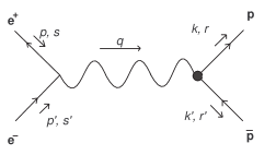
Figure 7.1: The one photon exchange diagram of the $e^{+}e^{-}\to p\bar{p}$ process.

The matrix element of the process $e^{+}e^{-}\to p\bar{p}$ in the framework of the one-photon exchange approximation to be presented in Fig. 7.1 is defined by the formulae

$$M = \frac{e^{2}}{k^{2}}j_{\mu}J_{\mu},$$

$$j_{\mu} = \bar{u}(-p)\gamma_{\mu}u(p^{\prime}),$$ (7.2)

$$J_{\mu} = \bar{u}(k)\bigl{[}F_{1p}(t)\gamma_{\mu}-F_{2p}(t)\frac{\sigma_{\mu\nu}k_{\nu}}{2m_{p}}\bigr{]}u(-k^{\prime}),$$

where $t=q^{2}\geq 4m_{p}^{2}$. We note, that the c.m. system of the reaction $e^{+}e^{-}\to p\bar{p}$ is the most suitable for the analysis of polarization effects.

The EM currents $j_{\mu}$ and $J_{\mu}$ are conserved $q\cdot j=q\cdot J=0$ and the matrix element $M$ is completely determined by the product of spatial components of the currents $\vec{j}$ and $\vec{J}$.

The electromagnetic current $\vec{J}$ can be expressed through two-component spinors $\varphi_{1}$ and $\varphi_{2}$

$$\vec{J}=\sqrt{t}\varphi^{+}_{1}\left[G_{Mp}(t)(\vec{\sigma}-\vec{n}\vec{\sigma}\cdot\vec{n})+\frac{2m_{p}}{\sqrt{t}}G_{Ep}(t)\vec{n}\vec{\sigma}\cdot\vec{n}\right]\varphi_{2},$$ (7.3)

where we denote

$$\vec{F}=\sqrt{t}\,[\,G_{Mp}(t)(\vec{\sigma}-\vec{n}\,\vec{\sigma}.\vec{n})+\frac{2m_{p}}{\sqrt{t}}\,G_{Ep}(t)\vec{n}\,\vec{\sigma}.\vec{n}\,],$$ (7.4)

$\vec{\sigma}$ are Pauli matrices, $\vec{n}=(0,0,1)$ is the unit vector along the three momentum $\vec{q}$ of the proton, $\vec{m}=(-\sin\vartheta,0,\cos\vartheta)$ is the unit vector of incoming electron (see Fig. 7.2) and $G_{Ep}(t)$ and $G_{Mp}(t)$ are defined by the relations (4.1).

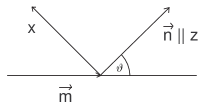
Figure 7.2: Definition of the scattering plane of the $e^{+}e^{-}\to p\bar{p}$ process

In order to find the corresponding cross-section, one has to calculate $|M|^{2}$. The differential cross section of the reaction $e^{+}e^{-}\to p\bar{p}$ in terms of EM FFs, for the case of unpolarized particles, has the form

$$\frac{d\sigma}{d\Omega}=\frac{\alpha^{2}}{4s}\left(\frac{1}{\tau}|G_{Ep}|^{2}\sin^{2}{\vartheta}+|G_{Mp}|^{2}[1+\cos^{2}{\vartheta}]\right),\;\quad\alpha=\frac{e^{2}}{4\pi};\quad\tau=\frac{t}{4m_{p}^{2}}.$$ (7.5)

Further single and double spin polarization observables are calculated explicitly.

First the single spin polarization observables (either for proton or for antiproton) in the case of

• unpolarized incoming leptons

• incoming electron to be longitudinally polarized.

are calculated.

In the case of unpolarized initial leptons the corresponding lepton tensor takes the form

$$j_{ij}=2t(\delta_{ij}-m_{i}m_{j})$$ (7.6)

and the vector polarization is

$$\vec{P}=\frac{j_{ij}Tr[F_{i}F_{j}^{\dagger}\vec{\sigma}]}{j_{ij}Tr[F_{i}F_{j}^{\dagger}]}.$$ (7.7)

Calculating the corresponding trace in the numerator, and similarly in the denominator, one obtains only $P_{y}$ component of the vector polarization to be nonzero

$$P_{x} = 0$$

$$P_{y} = \frac{\sin 2\vartheta\cdot Im[G^{*}_{Mp}(t)G_{Ep}(t)]}{\sqrt{\tau}[1/\tau|G_{Ep}|^{2}\sin^{2}\vartheta+|G_{Mp}|^{2}(1+\cos^{2}{\vartheta})]}$$ (7.8)

$$P_{z} = 0.$$

The y-axis is orthogonal to the scattering plane (see Fig. 7.2) defined by the unit vectors $\vec{m}$ and $\vec{n}$, along the three-momentum of the electron and along the three-momentum of the created proton, respectively.

The contributions of $P_{x}$ and $P_{z}$ in proton polarization are different from zero only if the electron (or positron) is longitudinally polarized, i.e. the lepton tensor takes the following form

$$j_{ij}=2t(\,\delta_{ij}-m_{i}m_{j}+\lambda i\varepsilon_{ijl}m_{l}\,).$$ (7.9)

Then the components of the vector polarization $\vec{P}$ of the created proton (or antiproton) in the reaction $e^{+}e^{-}\to p\bar{p}$ are

$$P_{x} = -\frac{2\sin\vartheta\cdot Re[G_{Ep}(t)G_{Mp}^{*}(t)]}{\sqrt{\tau}[1/\tau|G_{Ep}(t)|^{2}\sin^{2}\theta+|G_{Mp}(t)|^{2}(1+\cos^{2}\theta)]}$$ (7.10)

$$P_{y} = \frac{\sin{2\vartheta}\cdot Im[G^{*}_{Mp}(t)G_{Ep}(t)]}{\sqrt{\tau}[1/\tau|G_{Ep}(t)|^{2}\sin^{2}\vartheta+|G_{Mp}(t)|^{2}(1+\cos^{2}\vartheta)]}$$

$$P_{z} = \frac{2\cos\vartheta|G_{Mp}(t)|^{2}}{[1/\tau|G_{Ep}(t)|^{2}\sin^{2}\theta+|G_{Mp}(t)|^{2}(1+\cos^{2}\theta)]},$$

assuming $100\%$ longitudinal polarization of one of the leptons.

In a similar procedure one can find explicit forms of double spin polarization observables in the $e^{+}e^{-}\to p\bar{p}$ process, where we are interested for polarizations of created proton and antiproton simultaneously. The corresponding polarization tensor is

$$P_{kl}=\frac{j_{ij}Tr[F_{i}\sigma_{k}F_{j}^{\dagger}\sigma_{l}]}{j_{ij}Tr[F_{i}F_{j}^{\dagger}]},$$ (7.11)

where $k,l=x,y,z$. Calculating the trace in the numerator and similarly the trace in the denominator, considering unpolarized incoming leptons, one finds

$$P_{xx} = \sin^{2}\vartheta\cdot\frac{\tau|G_{Mp}(t)|^{2}+|G_{Ep}(t)|^{2}}{{\tau}[1/\tau|G_{Ep}(t)|^{2}\sin^{2}\vartheta+|G_{Mp}(t)|^{2}(1+\cos^{2}\vartheta)]};$$

$$P_{yy} = \sin^{2}\vartheta\cdot\frac{|G_{Ep}(t)|^{2}-{\tau}|G_{Mp}(t)|^{2}}{\tau[1/\tau|G_{Ep}(t)|^{2}\sin^{2}\vartheta+|G_{Mp}(t)|^{2}(1+\cos^{2}\vartheta)]};$$ (7.12)

$$P_{zz} = \frac{\tau(1+\cos^{2}{\vartheta})|G_{Mp}(t)|^{2}-sin^{2}{\vartheta}|G_{Ep}(t)|^{2}}{{\tau}[1/\tau|G_{Ep}(t)|^{2}\sin^{2}\vartheta+|G_{Mp}(t)|^{2}(1+\cos^{2}\vartheta)]};$$

$$P_{xy} = P_{yx}=0;$$

$$P_{xz} = P_{zx}=-\frac{\sin 2{\vartheta}Re[G^{*}_{Mp}(t)G_{Ep}(t)]}{\sqrt{\tau}[1/\tau|G_{Ep}(t)|^{2}\sin^{2}\vartheta+|G_{Mp}(t)|^{2}(1+\cos^{2}\vartheta)]};$$

$$P_{yz} = P_{zy}=0.$$

Now, if the expression (7.9) for the lepton tensor is used with the longitudinally polarized electron or positron, for components $P_{xx}$, $P_{yy}$, $P_{zz}$, $P_{xy}$, $P_{yx}$, $P_{xz}$, $P_{zx}$ one obtains identical expressions with (7.12), but the last two components are now nonzero as well

$$P_{yz}=P_{zy}=\frac{\sin\vartheta Im[G^{*}_{Mp}(t)G_{Ep}(t)]}{\sqrt{\tau}[1/\tau|G_{Ep}(t)|^{2}\sin^{2}\vartheta+|G_{Mp}(t)|^{2}(1+\cos^{2}\vartheta)]}.$$ (7.13)

Every of components $P_{kl}$ characterize a polarization of the proton $p$ in the direction $k$, if antiproton $\bar{p}$ is polarized at the direction $l$ and they all are calculated for $100\%$ polarization of one of the initial leptons.

As one can see from explicit formulae the vector polarization component $P_{y}$ and the tensor polarization components $P_{xz}$=$P_{zx}$ depend on the imaginary parts of electric and magnetic proton FFs. So, only our $U\&A$ models of the nucleon EM structure can give a sophisticate prediction of behaviors of $P_{y}$ and $P_{xz}$=$P_{zx}$. The eight and ten resonance U&A models represent compatible unification of pole and continua (in the language of the analyticity given by cuts on positive real axis) contributions, which give just imaginary parts of FFs different from zero starting always from the lowest branch point representing the lowest opened physical threshold.

Now, exploiting behaviors of proton electric and magnetic FFs in the time-like region as predicted by our eight and ten-resonance $U\&A$ models one finds [160] behaviors of single and double spin polarization observables of the $e^{+}e^{-}\to p\bar{p}$ process as they are presented in figures Fig. 7.3, 7.4.

Figure 7.3: Prediction of the single polarizations observables by ten-resonance (left-hand) and eight-resonance (right-hand) U&A model

Figure 7.4: Prediction of the double polarizations observables by ten-resonance (left-hand) and eight-resonance (right-hand) U&A model

7.2 Polarization effects in $e^{+}e^{-}\rightarrow d\bar{d}$ and experimental determination of time like deuteron form factors

In the present paragraph the polarization observables in the reaction

$$e^{-}(k_{1})+e^{+}(k_{2})\rightarrow d(p_{1})+\bar{d}(p_{2}),$$ (7.14)

where the momenta of the particles are indicated in brackets, are calculated [161] explicitly.

With this aim one considers the case of unpolarized and longitudinally-polarized electron beam with production of vector- and tensor-polarized deuterons. The expressions of polarization observables are given in terms of the deuteron EM FFs in time-like region, where they are complex functions of the momentum transfer squared.

In the one-photon approximation, the differential cross section of the reaction (7.14) in terms of the leptonic $L_{\mu\nu}$ and hadronic $W_{\mu\nu}$ tensors contraction (in the Born approximation one can neglect the electron mass) is written as

$$\frac{d\sigma}{d\Omega}=\frac{\alpha^{2}\beta}{4q^{2}}\frac{L_{\mu\nu}W_{\mu\nu}}{q^{4}},$$ (7.15)

where $\alpha=1/137$ is the electromagnetic constant, $\beta=\sqrt{1-4m_{d}^{2}/q^{2}}$ is the deuteron velocity in the reaction center of mass system (CMS), $m_{d}$ is the deuteron mass and $q$ is the four momentum of the virtual photon, $q=k_{1}+k_{2}=p_{1}+p_{2}$ (note that the cross section is not averaged over the spins of the initial beams).

The leptonic tensor (for the case of longitudinally polarized electron beam) is

$$L_{\mu\nu}=-q^{2}g_{\mu\nu}+2(k_{1\mu}k_{2\nu}+k_{2\mu}k_{1\nu})+2i\lambda\varepsilon_{\mu\nu\sigma\rho}k_{1\sigma}k_{2\rho}\ ,$$ (7.16)

where $\lambda$ is the degree of the beam polarization (further we assume that the electron beam is completely polarized and consequently $\lambda=1$).

The hadronic tensor can be expressed via the deuteron electromagnetic current $J_{\mu}$, describing the transition $\gamma^{*}\rightarrow\bar{d}d$, as

$$W_{\mu\nu}=J_{\mu}J^{*}_{\nu}\ .$$ (7.17)

As the deuteron is a spin-one nucleus, its electromagnetic current is completely described by three FFs. Assuming the P and C invariance of the hadron EM interaction this current can be decomposed (2.19) into three deuteron EM FFs $F_{1}$, $F_{2}$ and $F_{3}$, by means of which analogically to the nucleon Sachs EM FFs $G_{Cd}$, $G_{Md}$ and $G_{Qd}$ (2.20) are defined .

When calculating the expression for the hadron tensor $W_{\mu\nu}$ in terms of the deuteron electromagnetic FFs, the spin-density matrices of the deuteron and antideuteron to be defined by means of deuteron polarization vectors $\xi$ and $\xi*$ are

$$\xi_{1\mu}\xi^{*}_{1\nu} = -\left(g_{\mu\nu}-\frac{p_{1\mu}p_{1\nu}}{m_{d}^{2}}\right)+\frac{3i}{2m_{d}}\varepsilon_{\mu\nu\rho\sigma}s_{\rho}p_{1\sigma}+3Q_{\mu\nu}$$ (7.18)

$$\xi_{2\mu}\xi^{*}_{2\nu} = -\left(g_{\mu\nu}-\frac{p_{2\mu}p_{2\nu}}{m_{d}^{2}}\right)$$

if the deuteron polarization is measured and the antideuteron polarization is not measured. Here $s_{\mu}$ and $Q_{\mu\nu}$ are the deuteron polarization four vector and quadrupole tensor, respectively. The four vector of the deuteron vector polarization $s_{\mu}$ and the deuteron quadrupole-polarization tensor $Q_{\mu\nu}$ satisfy the following conditions

$$s^{2}=-1,\;sp_{1}=0,\;Q_{\mu\nu}=Q_{\nu\mu},\quad Q_{\mu\mu}=0,\;p_{1\mu}Q_{\mu\nu}=0.$$

Taking into account Eqs. (7.17) and (7.18), the hadronic tensor in the general case can be written as the sum of three terms

$$W_{\mu\nu}=W_{\mu\nu}(0)+W_{\mu\nu}(V)+W_{\mu\nu}(T),$$ (7.19)

where $W_{\mu\nu}(0)$ corresponds to the case of unpolarized deuteron and $W_{\mu\nu}(V)$ $(W_{\mu\nu}(T))$ corresponds to the case of the vector (tensor) polarized deuteron. The explicit form of these terms is

- the unpolarized term $W_{\mu\nu}(0)$:

$$W_{\mu\nu}(0) = W_{1}(q^{2})\tilde{g}_{\mu\nu}+\frac{W_{2}(q^{2})}{m_{d}^{2}}\tilde{p}_{1\mu}\tilde{p}_{1\nu}$$

$$\tilde{g}_{\mu\nu} = g_{\mu\nu}-\frac{q_{\mu}q_{\nu}}{q^{2}}\quad\tilde{p}_{1\mu}=p_{1\mu}-\frac{p_{1}q}{q^{2}}q_{\mu}$$

$$W_{1}(q^{2}) = 8m_{d}^{2}\tau(1-\tau)|G_{Md}|^{2},$$

$$W_{2}(q^{2}) = 12m_{d}^{2}(|G_{Cd}|^{2}-\frac{2}{3}\tau|G_{Md}|^{2}+\frac{8}{9}\tau^{2}|G_{Qd}|^{2})$$ (7.20)

and $\tau=-q^{2}/{4m_{d}^{2}}$.

- the term for vector polarization $W_{\mu\nu}(V)$:

$$W_{\mu\nu}(V) = \frac{i}{m_{d}}S_{1}(q^{2})\varepsilon_{\mu\nu\sigma\rho}s_{\sigma}q_{\rho}+\frac{i}{m_{d}^{3}}S_{2}(q^{2})[\tilde{p}_{1\mu}\varepsilon_{\nu\alpha\sigma\rho}s_{\alpha}q_{\sigma}p_{1\rho}-\tilde{p}_{1\nu}\varepsilon_{\mu\alpha\sigma\rho}s_{\alpha}q_{\sigma}p_{1\rho}]+$$ (7.21)

$$+ \frac{1}{m_{d}^{3}}S_{3}(q^{2})[\tilde{p}_{1\mu}\varepsilon_{\nu\alpha\sigma\rho}s_{\alpha}q_{\sigma}p_{1\rho}+\tilde{p}_{1\nu}\varepsilon_{\mu\alpha\sigma\rho}s_{\alpha}q_{\sigma}p_{1\rho}],$$

$$S_{1}(q^{2}) = -3m_{d}^{2}(\tau-1)|G_{Md}|^{2},$$

$$S_{2}(q^{2}) = 3m_{d}^{2}[|G_{Md}|^{2}-2Re(G_{Cd}-\frac{\tau}{3}G_{Qd})G_{Md}^{*}],$$

$$S_{3}(q^{2}) = 6m_{d}^{2}Im(G_{Cd}-\frac{\tau}{3}G_{Qd})G_{Md}^{*}.$$

- the term for tensor polarization $W_{\mu\nu}(T)$:

$$W_{\mu\nu}(T) = V_{1}(q^{2})\bar{Q}\tilde{g}_{\mu\nu}+V_{2}(q^{2})\frac{\bar{Q}}{m_{d}^{2}}\tilde{p}_{1\mu}\tilde{p}_{1\nu}+$$

$$+ V_{3}(q^{2})(\tilde{p}_{1\mu}\widetilde{Q}_{\nu}+\tilde{p}_{1\nu}\widetilde{Q}_{\mu})+V_{4}(q^{2})\widetilde{Q}_{\mu\nu}\ +iV_{5}(q^{2})(\tilde{p}_{1\mu}\widetilde{Q}_{\nu}-\tilde{p}_{1\nu}\widetilde{Q}_{\mu}),$$

where

$$\widetilde{Q}_{\mu} = Q_{\mu\nu}q_{\nu}-\frac{q_{\mu}}{q^{2}}\bar{Q}\,\widetilde{Q}_{\mu}q_{\mu}=0$$

$$\widetilde{Q}_{\mu\nu} = Q_{\mu\nu}+\frac{q_{\mu}q_{\nu}}{q^{4}}\bar{Q}-\frac{q_{\nu}q_{\alpha}}{q^{2}}Q_{\mu\alpha}-\frac{q_{\mu}q_{\alpha}}{q^{2}}Q_{\nu\alpha}\,\widetilde{Q}_{\mu\nu}q_{\nu}=0,$$

$$\bar{Q} = Q_{\alpha\beta}q_{\alpha}q_{\beta}.$$ (7.23)

The tensor structure functions $V_{i}(q^{2})$ are combinations of deuteron FFs as follows

$$V_{1}(q^{2}) = -3|G_{Md}|^{2},$$

$$V_{2}(q^{2}) = 3\left[|G_{Md}|^{2}+\frac{4}{1-\tau}Re(G_{Cd}-\frac{\tau}{3}G_{Qd}-\tau G_{Md})G_{Qd}^{*}\right],$$

$$V_{3}(q^{2}) = -6\tau\left[|G_{Md}|^{2}+2ReG_{Qd}G_{Md}^{*}\right],$$ (7.24)

$$V_{4}(q^{2}) = -12m_{d}^{2}\tau(1-\tau)|G_{Md}|^{2},\quad V_{5}(q^{2})=-12\tau Im(G_{Qd}G_{Md}^{*}).$$

Using the definitions of the cross–section (7.15), leptonic (7.16) and hadronic (7.19) tensors, one can easily derive the expression for the unpolarized differential cross section in terms of the structure functions $W_{1,2}$ (after averaging over the spins of the initial particles)

$$\frac{d\sigma^{un}}{d\Omega}=\frac{\alpha^{2}\beta}{4q^{4}}\left\{-W_{1}(q^{2})+\frac{1}{2}W_{2}(q^{2})\left[\tau-1-\frac{(u-t)^{2}}{4m_{d}^{2}q^{2}}\right]\right\}\ ,$$ (7.25)

where $t=(k_{1}-p_{1})^{2}$, $u=(k_{1}-p_{2})^{2}.$

In the reaction CMS this expression can be written as

$$\frac{d\sigma^{un}}{d\Omega}=\frac{\alpha^{2}\beta^{3}}{4q^{2}}D,\ D=\tau(1+\cos^{2}\theta)|G_{Md}|^{2}+\frac{3}{2}\sin^{2}\theta\left(|G_{Cd}|^{2}+\frac{8}{9}\tau^{2}|G_{Qd}|^{2}\right),$$ (7.26)

where $\theta$ is the angle between the momenta of the deuteron (${\vec{p}}$) and the electron beam (${\vec{k}}$). Integrating the expression (7.26) with respect to the deuteron angular variables one obtains the following formula for the total cross section of the reaction (7.14)

$$\sigma_{tot}(e^{+}e^{-}\to\bar{d}d)=\frac{\pi\alpha^{2}\beta^{3}}{3q^{2}}\biggl{[}3|G_{Cd}|^{2}+4\tau(|G_{Md}|^{2}+\frac{2}{3}\tau|G_{Qd}|^{2})\biggr{]}.$$ (7.27)

One can define also an angular asymmetry, $R$, with respect to the differential cross section measured at $\theta=\pi/2,\sigma_{0}$

$$\frac{d\sigma^{un}}{d\Omega}=\sigma_{0}(1+Rcos^{2}\theta),$$ (7.28)

where $R$ can be expressed as a function of the deuteron FFs

$$R=\frac{2\tau(|G_{M}|^{2}-\frac{4}{3}\tau|G_{Q}|^{2})-3|G_{C}|^{2}}{2\tau(|G_{M}|^{2}+\frac{4}{3}\tau|G_{Q}|^{2})+3|G_{C}|^{2}}.$$ (7.29)

This observable should be sensitive to the different underlying assumptions on deuteron FFs; therefore, a precise measurement of this quantity, which does not require polarized particles, would be very interesting.

One can see from (7.26) that, as in the space-like region, the measurement of the angular distribution of the outgoing deuteron determines the modulus of the magnetic FF. The separation of the charge and quadrupole FFs requires the measurement of polarization observables to be more convenient derived in CMS. When considering the polarization of the final particle, we choose a reference system with the $z$ axis along the momentum of this particle (in our case it is ${\vec{p}}$). The $y$ axis is normal to the reaction plane in the direction of ${\vec{k}}\times{\vec{p}}$, $x$, $y$ and $z$ form a right-handed coordinate system.

The cross section can be written, in the general case, as the sum of unpolarized and polarized terms, corresponding to the different polarization states and polarization directions of the incident and scattered particles

$$\frac{d\sigma}{d\Omega}=\displaystyle\frac{d\sigma^{un}}{d\Omega}\left[1+P_{y}+\lambda P_{x}+\lambda P_{z}+P_{zz}R_{zz}+P_{xz}R_{xz}+P_{xx}(R_{xx}-R_{yy})+\lambda P_{yz}R_{yz}\right],$$ (7.30)

where $P_{i}$ ($P_{ij}$), $i,j=x,y,z$ are the components of the polarization vector (tensor) of the outgoing deuteron, $R_{ij}$, $i,j=x,y,z$ the components of the quadrupole polarization tensor of the outgoing deuteron $Q_{\mu\nu}$, in its rest system and $\displaystyle\frac{d\sigma^{un}}{d\Omega}$ is the differential cross-section for the unpolarized case.

The degree of longitudinal polarization of the electron beam, $\lambda$, is explicitly indicated, in order to stress the origin of the specific polarization observables.

Now, let us consider the different polarization observables and give their expression in terms of the deuteron EM FFs.

• The vector polarization of the outgoing deuteron, $P_{y}$, which does not require polarization in the initial state is

  $$P_{y}=-\frac{3}{2}\sqrt{\tau}\sin(2\theta)Im\left[\left(G_{Cd}-\frac{\tau}{3}G_{Qd}\right)G_{Md}^{*}\right]$$ (7.31)

• The part of the differential cross section that depends on the tensor polarization can be written as follows

  $$\displaystyle\frac{d\sigma_{T}}{d\Omega} =\frac{d\sigma_{zz}}{d\Omega}R_{zz}+\frac{d\sigma_{xz}}{d\Omega}R_{xz}+\frac{d\sigma_{xx}}{d\Omega}(R_{xx}-R_{yy}),$$ (7.32)

  $$\displaystyle\frac{d\sigma_{zz}}{d\Omega} =\frac{\alpha^{2}\beta^{3}}{4q^{2}}\frac{3\tau}{4}\left[(1+\cos^{2}\theta)|G_{Md}|^{2}+8\sin^{2}\theta\left(\frac{\tau}{3}|G_{Qd}|^{2}-Re(G_{Cd}.G_{Qd}^{*})\right)\right],$$

  $$\displaystyle\frac{d\sigma_{xz}}{d\Omega} =-\frac{\alpha^{2}\beta^{3}}{4q^{2}}3\tau^{3/2}\sin(2\theta)Re(G_{Qd}.G_{Md}^{*}),$$

  $$\displaystyle\frac{d\sigma_{xx}}{d\Omega} =-\frac{\alpha^{2}\beta^{3}}{4q^{2}}\frac{3\tau}{4}\sin^{2}\theta|G_{Md}|^{2},$$

• Let us consider now the case of a longitudinally polarized electron beam. The other two components of the deuteron vector polarization ($P_{x}$, $P_{z}$) require the initial particle polarization and are

  $$P_{x}=-3\frac{\sqrt{\tau}}{D}\sin\theta Re\left(G_{Cd}-\frac{\tau}{3}G_{Qd}\right)G_{Md}^{*},\ P_{z}=\frac{3\tau}{2D}\cos\theta|G_{Md}|^{2}.$$ (7.33)

From angular momentum and helicity conservations it follows that the sign of the deuteron polarization component $P_{z}$ in the forward direction ($\theta=\leavevmode\nobreak\ 0$) must coincide with the sign of the electron beam polarization. This requirement is satisfied by Eq. (7.33).

A possible nonzero phase difference between the deuteron FFs leads to another T-odd polarization observable proportional to the $R_{yz}$ component of the tensor polarization of the deuteron. The part of the differential cross section that depends on the correlation between the longitudinal polarization of the electron beam and the deuteron tensor polarization can be written as follows

$$\frac{d\sigma_{\lambda T}}{d\Omega}=\frac{\alpha^{2}\beta^{3}}{4q^{2}}6\tau^{3/2}\sin\theta Im(G_{Md}.G_{Qd}^{*})R_{yz}.$$ (7.34)

The deuteron FFs in the time-like region are complex functions. In the case of unpolarized initial and final particles, the differential cross section depends only on the squared modulus $|G_{Md}|^{2}$ and on the combination $G=|G_{Cd}|^{2}+\frac{8}{9}\tau^{2}|G_{Qd}|^{2}.$ So, the measurement of the angular distribution allows one to determine $|G_{Md}|$ and the quantity $G$, as in the elastic electron-deuteron scattering.

Let us discuss, which information can be obtained by measuring the polarization observables derived above. Three relative phases exist for three deuteron EM FFs, which we note as follows: $\alpha_{1}=\alpha_{M}-\alpha_{Q},$ $\alpha_{2}=\alpha_{M}-\alpha_{C},$ and $\alpha_{3}=\alpha_{Q}-\alpha_{C},$ where $\alpha_{M}=ArgG_{Md},$ $\alpha_{C}=ArgG_{Cd},$ and $\alpha_{Q}=ArgG_{Qd}.$ These phases are important characteristics of FFs in the time-like region since they result from the strong interaction between final particles.

Let us consider the ratio of the polarizations $P_{yz}$ (we would like to note that it requires a longitudinally polarized electron beam) and $P_{xz}$ (when the electron beam is unpolarized). One finds

$$R_{1}=\frac{P_{xz}}{P_{yz}}=-\cos\theta\cot\alpha_{1}.$$ (7.35)

So, the measurement of this ratio gives us information about the relative phase $\alpha_{1}$. The measurement of another ratio of polarizations, $R_{2}=P_{xz}/P_{xx}$ gives us information about the quantity $|G_{Qd}|$

$$R_{2}=\frac{P_{xz}}{P_{xx}}=8\sqrt{\tau}\cot\theta\cos\alpha_{1}\frac{|G_{Qd}|}{|G_{Md}|}.$$ (7.36)

This allows one to obtain the modulus of the charge FF, $|G_{Cd}|$, from the quantity $G$, known from the measurement of the differential cross section. The measurement of a third ratio

$$R_{3}=\frac{P_{y}}{P_{x}}=-\cos\theta\frac{\sin\alpha_{2}-r\sin\alpha_{1}}{\cos\alpha_{2}-r\cos\alpha_{1}},\ \ r=\frac{\tau}{3}\frac{|G_{Qd}|}{|G_{Cd}|}$$ (7.37)

allows to determine the phase difference $\alpha_{2}$. And at last, if we measure the ratio of the polarizations $P_{zz}$ and $P_{xx}$

$$R_{4}=\frac{P_{zz}}{P_{xx}}=-\frac{1}{\sin^{2}\theta}\left[1+\cos^{2}\theta+8\sin^{2}\theta\frac{|G_{Cd}||G_{Qd}|}{|G_{Md}|^{2}}(r-\cos\alpha_{3})\right]$$ (7.38)

we can obtain information about the third phase difference $\alpha_{3}$. Moreover, one can verify the relation:

$$\alpha_{3}=\alpha_{2}-\alpha_{1}.$$

Thus, the measurement of the polarization observables in the process (7.14) allows to determine the deuteron EM FFs in the time-like region for the firs time.

7.3 Alternative method of experimental determination of deuteron electromagnetic form factors

In 4.3 we have demonstrated that alternative method of a measurement of the same physical quantity, in this case the proton electric FF $G_{Ep}(t)$, can lead to very surprising results. To be motivated by means of this example, here we propose [162] to experimentalists a new method of experimental measurement of all three deuteron EM FFs in the space-like region for the first time.

Knowing experimentally the FFs (2.19) $F_{1}(t)$, $F_{2}(t)$ and $F_{3}(t)$, one can specify experimental behaviors of $G_{C}(t)$, $G_{M}(t)$ and $G_{Q}(t)$ by (2.20).

The FF $F_{2}(t)$ can be found by a measurement of the unpolarized differential cross-section in the laboratory system

$$\frac{d\sigma_{unp}^{Lab}}{d\Omega}=\frac{1}{64\pi^{2}m_{d}^{2}}\bigg{[}\frac{1}{1+(2E_{e}/m_{d})\sin^{2}(\theta/2)}\bigg{]}^{2}|\mathcal{M}|_{\text{unp}}^{2}$$ (7.39)

with

$$|\mathcal{M}|_{\text{unp}}^{2}=\frac{e^{4}m_{d}^{2}}{E^{2}_{e}}\frac{\cos^{2}(\theta/2)}{\sin^{4}(\theta/2)}\bigg{(}1+(2E_{e}/m_{d})\sin^{2}(\theta/2)\bigg{)}\bigg{[}A(t)+B(t)\tan^{2}(\theta/2)\bigg{]},$$ (7.40)

and deuteron elastic structure functions (2.22).

In order to find $F_{1}(t)$, we suggest to measure elastic electron-deuteron scattering with only vector polarized deuterons, where the incoming (target) deuteron is polarized in the direction $\vec{n}$ of the three momenta of outgoing deuteron and the vector polarization of the outgoing deuteron has the same direction. Then in the laboratory system (the rest frame of the incoming deuteron) the four vectors of electron and deuteron momenta ($k_{1}$, $p_{1}$, $p_{2}$) and the deuteron vector polarizations $\xi_{1}$, $\xi_{2}$ can be expressed in components as

$$k_{1}=(E_{e},0,0,E_{e});\quad\quad p_{1} = (m_{d},0,0,0);\quad\quad p_{2}=(E_{2},|\vec{p}_{2}|\vec{n});$$

$$\xi_{1} = (0,\vec{n});\quad\quad\xi_{2}=\frac{1}{m_{d}}(|\vec{p}_{2}|,E_{2}\vec{n});$$

$$|\vec{p}_{2}| = 2m_{d}\sqrt{\eta(1+\eta)};\quad\quad E_{2}=m_{d}(1+2\eta),$$ (7.41)

where the outgoing deuteron vector polarization was obtained by Lorentz boost to be the kinematic frame of the recoil deuteron. As a result one obtains the following relations

$$(\xi_{1}\cdot\xi_{2}) = -1-2\eta;\quad\quad(\xi_{1}\cdot p_{2})=-|\vec{p}_{2}|;\quad\quad(\xi_{2}\cdot p_{1})=|\vec{p}_{2}|;$$

$$(\xi_{1}\cdot k_{1})(\xi_{2}\cdot p_{1}) = -2m_{d}(E_{e}+m_{d})\eta;$$

$$(\xi_{1}\cdot k_{1})(\xi_{2}\cdot k_{1}) = \frac{\eta}{1+\eta}(E_{e}+m_{d})[m_{d}(1+2\eta)-E_{e}];$$

$$(p_{1}\cdot k_{1}) = \quad E_{e}m_{d};\quad\quad(p_{1}\cdot p_{2})=m_{d}^{2}(1+2\eta)$$ (7.42)

to be useful in further calculations.

The absolute value squared for the amplitude of the polarized elastic electron-deuteron scattering is

$$|\mathcal{M}|_{\uparrow\uparrow}^{2} = \frac{e^{4}}{q^{4}}(2k_{1\mu}k_{2\nu}+2k_{1\nu}k_{2\mu}+g_{\mu\nu}q^{2})\sum_{spins}\bigg{\{}\Big{[}-F_{1}(\xi_{2}^{*}\cdot\xi_{1})+$$ (7.43)

$$+ F_{3}\frac{(\xi_{2}^{*}\cdot q)(\xi_{1}\cdot q)}{2m_{d}^{2}}\Big{]}(p_{1}^{\mu}+p_{2}^{\mu})-F_{2}\Big{[}\xi_{1}^{\mu}(\xi_{2}^{*}\cdot q)-\xi_{2}^{*\mu}(\xi_{1}\cdot q)\Big{]}\bigg{\}}\times$$

$$\times \bigg{\{}\Big{[}-F_{1}(\xi_{2}\cdot\xi_{1}^{*})+F_{3}\frac{(\xi_{2}\cdot q)(\xi_{1}^{*}\cdot q)}{2m_{d}^{2}}\Big{]}(p_{1}^{\nu}+p_{2}^{\nu})-$$

$$- G_{2}\Big{[}\xi_{1}^{*\nu}(\xi_{2}\cdot q)-\xi_{2}^{\mu}(\xi_{1}^{*}\cdot q)\Big{]}\bigg{\}},$$

then by using properties of the deuteron polarization vectors $\xi_{1}$ , $\xi_{2}$, (7.41) and (7.42), it can be arranged by the computer program FORM and simplified by Maxima to the form

$$|\mathcal{M}|_{\uparrow\uparrow}^{2}=\frac{1}{3}\frac{e^{4}m^{2}_{d}}{E_{e}^{2}}\frac{\cos^{2}(\theta/2)}{\sin^{4}(\theta/2)}\bigg{(}1+(2E_{e}/m_{d})\sin^{2}(\theta/2)\bigg{)}\bigg{[}A(t)+B(t)\tan^{2}(\theta/2)+\frac{3}{2}F^{2}_{1}(t)\bigg{]}.$$ (7.44)

In the latter equation one can identify the absolute value squared of the unpolarized matrix element (7.40) and as a result one obtains

$$|\mathcal{M}|_{\uparrow\uparrow}^{2}=\frac{1}{3}|\mathcal{M}|_{\text{unp}}^{2}+\frac{e^{4}m_{d}^{2}}{2E^{2}_{e}}\frac{\cos^{2}(\theta/2)}{\sin^{4}(\theta/2)}\bigg{(}1+(2E_{e}/{m_{d}})\sin^{2}(\theta/2)\bigg{)}F_{1}^{2}(t).$$ (7.45)

Multiplying the relation (7.45) by

$$\frac{1}{64\pi^{2}m_{d}^{2}}\bigg{(}\frac{1}{1+(2{E_{e}}/{m_{d}})\sin^{2}(\theta/2)}\bigg{)}^{2}$$

one comes to the equation

$$\frac{d\sigma_{\uparrow\uparrow}^{Lab}}{d\Omega}-\frac{1}{3}\frac{d\sigma^{Lab}_{unp}}{d\Omega}=\frac{\alpha^{2}}{8E^{2}_{e}}\frac{\cos^{2}(\theta/2)}{\sin^{4}(\theta/2)}\frac{1}{1+(2{E_{e}}/{m_{d}})\sin^{2}(\theta/2)}F_{1}^{2}(t).$$ (7.46)

from which the EM FF $F_{1}(t)$ can be extracted.

The third FF $F_{3}(t)$ is given by a solution of the quadratic equation

$$\bigg{[}\frac{12}{9}\eta^{2}(1+\eta^{2}\bigg{]}F_{3}^{2}(t)+$$

$$+ \bigg{[}\frac{4}{3}\eta(1+\eta)F_{1}(t)+\frac{16}{9}\eta^{2}(1+\eta)(F_{1}(t)-F_{2}(t))\bigg{]}\cdot F_{3}(t)+$$

$$+ \bigg{\{}\Big{[}F_{1}(t)+\frac{2}{3}\eta(F_{1}(t)-F_{2}(t))\Big{]}^{2}+\frac{2}{3}\eta F_{2}^{2}(t)+\frac{8}{9}\eta^{2}(F_{1}(t)-F_{2}(t))^{2}-A(t)\bigg{\}}=0$$

(with $\eta=t/{4m_{d}^{2}}$) to be obtained by a substitution of (2.20) into the first relation of (2.22).

Ones the data on $F_{1}(t)$, $F_{2}(t)$ and $F_{3}(t)$ are known, by using (2.20) one can obtain the experimental behavior of $G_{C}(t)$, $G_{M}(t)$ and $G_{Q}(t)$.

8 Muon anomalous magnetic moment

The muon is described by the Dirac equation and its magnetic moment is related to the spin by means of the expression

$$\vec{\mu}=g\left({e\over 2m_{\mu}}\right)\vec{s}$$ (8.1)

where the value of gyromagnetic ratio $g$ is predicted (in the absence of the Pauli term) to be exactly 2.

However, interactions existing in nature modify $g$ to be exceeding the value 2 because of the emission and absorption of

• virtual photons (electromagnetic effects),

• intermediate vector and Higgs bosons (weak interaction effects)

• vacuum polarization into virtual hadronic states (strong interaction effects).

In order to describe this modification of $g$ theoretically, the magnetic anomaly was introduced by the relation

$$a_{\mu}\equiv\frac{g-2}{2} = a_{\mu}^{(1)}\left({\alpha\over\pi}\right)+\left(a_{\mu}^{(2)QED}+a_{\mu}^{(2)had}\right)\left({\alpha\over\pi}\right)^{2}+$$ (8.2)

$$+ a_{\mu}^{(2)weak}+O\left({\alpha\over\pi}\right)^{3}$$

where to every order some Feynman diagrams (see Figs. 8.1-8.3) correspond and

$$\alpha=1/137.03599976(50)$$

is the fine structure constant.

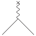
Figure 8.1: The simplest Feynman diagram of an interaction of the muon with an external magnetic field.

Figure 8.2: The lowest-order hadronic vacuum-polarization contribution to the anomalous magnetic moment of the muon.

Figure 8.3: The third-order hadronic vacuum-polarization contributions to the anomalous magnetic moment of the muon.

The muon anomalous magnetic moment $a_{\mu}$ is very interesting object for theoretical investigations due to the following reasons

1. it is one of the best measured quantities (BNL E-821 experiment) in physics [163]

   $$a_{\mu}^{exp}=(116592040\pm 86)\times 10^{-11}$$ (8.3)

2. its accurate theoretical evaluation provides an extremely clean test of ”Electroweak theory” and may give hints on possible deviations from Standard Model (SM)

3. moreover, in near future the measurement in BNL is expected to be performed yet with an improved accuracy

   $$\Delta a_{\mu}^{exp}=\pm 40\times 10^{-11}$$ (8.4)

   i.e. it is aimed at obtaining a factor 2 in a precision above that of the last E-821 measurements.

At the aimed level of the precision (8.4) a sensibility will already exist to contributions

$$a_{\mu}^{(2,3)weak}=(152\pm 4)\times 10^{-11},$$ (8.5)

arising from single- and two-loop weak interaction diagrams. And so, if we compare theoretical evaluations of QED contributions up to 8th order

$a_{\mu}^{QED}=(116584705.7\pm 2.9)\times 10^{-11}$[164]

the single- and two-loop weak contributions

$a_{\mu}^{(2,3)weak}=(151\pm 4)\times 10^{-11}$[165]

$a_{\mu}^{(2,3)weak}=(153\pm 3)\times 10^{-11}$[166]

$a_{\mu}^{(2,3)weak}=(152\pm 1)\times 10^{-11}$[167]

strong interaction contributions

$a_{\mu}^{had}=(7068\pm 172)\times 10^{-11}$[168]

$a_{\mu}^{had}=(7100\pm 116)\times 10^{-11}$[169]

$a_{\mu}^{had}=(7052\pm 76)\times 10^{-11}$[170]

$a_{\mu}^{had}=(7024\pm 152)\times 10^{-11}$[171]

$a_{\mu}^{had}=(7021\pm 76)\times 10^{-11}$[172]

it is straightforward to see that the largest uncertainty is in $a_{\mu}^{had}$.

Error is comparable, or in the best case two times smaller than the weak interaction contributions.

So, in order to test the SM predictions for $a_{\mu}$ and to look for new physics in comparison with BNL E-821 experiment, one has still to improve an evaluation of $a_{\mu}^{had}$ and its error.

The most critical from all hadronic contributions are the light-by-light (LBL) contributions (see Fig. 8.4) to be approximated by a sum of meson pole terms (see Fig. 8.5).

Figure 8.4: Third order hadronic light-by-light scattering contribution to $a_{\mu}^{had}$ ($\mathcal{A}$) and class of pseudoscalar meson square loop diagrams ($\mathcal{B}$) and quark square loop diagrams ($\mathcal{C}$) contributing to ($\mathcal{A}$).

Figure 8.5: Meson pole terms contribution to LBL diagram

Therefore, we have recalculated [173] the third-order hadronic LBL contributions to the anomalous magnetic moment of the muon $a_{\mu}^{had}$ from the pole terms of the scalar $\sigma$, $a_{0}$ and pseudoscalar $\pi^{0}$, $\eta$, $\eta^{\prime}$ mesons $(M)$ in the framework of the linearized extended Nambu-Jona-Lasinio model

$\mathcal{L}_{q\bar{q}M}=g_{M}\bar{q}(x)\left[\sigma(x)+i\pi(x)\gamma_{5}\right]q(x).$

The reason for the latter are predictions of series of recent papers

$a_{\mu}^{LBL}=(+52\pm 18)\times 10^{-11}$[174]

$a_{\mu}^{LBL}=(+92\pm 32)\times 10^{-11}$[175]

$a_{\mu}^{LBL}=(+83\pm 12)\times 10^{-11}$[176]

$a_{\mu}^{LBL}(\pi_{0})=(+58\pm 10)\times 10^{-11}$[177]

which differ in the magnitude.

Moreover, in these papers only the pseudoscalar meson pole contributions were considered. We include the scalar meson $(\sigma,a_{0})$ pole contributions as well.

Current methods in a description of the $\gamma^{*}\rightarrow M\gamma^{*}$ transition form factors are ChPT and the vector-meson-dominance (VMD) model.

Here the corresponding transition form factors by the constituent quark triangle loops (see Fig. 8.5) with colorless and flavorless quarks with charge equal to the electron one are represented.

An application of a similar modified constituent quark triangle loop model for a prediction of the pion electromagnetic form factor behavior was carried out in [178] where also a comparison with the naive VMD model prediction was demonstrated.

The mass of the quark in the triangle loop is taken to be

$m_{u}=m_{d}=m_{q}=(280\pm 20)$ MeV

determined [179] in the framework of the chiral quark model of the Nambu-Jona-Lasinio type by exploiting the experimental values of the pion decay constant, the $\rho$-meson decay into two-pions constant, the masses of pion and kaon and the mass difference of $\eta$ and $\eta^{\prime}$ mesons.

The unknown strong coupling constants of $\pi^{0},\eta,\eta^{\prime}$ and $a_{0}$ mesons with quarks are evaluated in a comparison of the corresponding theoretical two-photon widths with experimental ones.

The $\sigma$-meson coupling constant is taken to be equal to $\pi^{0}$-meson coupling constant as it follows from the corresponding Lagrangian.

The $\sigma$-meson mass is taken to be $m_{\sigma}$=$(496\pm 47)$ MeV as an average of the values recently obtained experimentally from the decay $D^{+}\rightarrow\pi^{-}\pi^{+}\pi^{+}$ [180] and excited $\Upsilon$ decay [181] processes.

As a result we present explicit formulas for $a_{\mu}^{LBL}(M)$ $(M=\pi^{0},\eta,\eta^{\prime},\sigma,a_{0})$ in terms of Feynman parametric integrals of 10-dimensional order, which subsequently are calculated by MIKOR method.

Finally, one finds

$$a_{\mu}^{LBL}(\pi^{0}) = (81.83\pm 16.50)\times 10^{-11}$$ (8.6)

$$a_{\mu}^{LBL}(\eta) = (5.62\pm 1.25)\times 10^{-11}$$

$$a_{\mu}^{LBL}(\eta^{\prime}) = (8.00\pm 1.74)\times 10^{-11}$$

$$a_{\mu}^{LBL}(\sigma) = (11.67\pm 2.38)\times 10^{-11}$$

$$a_{\mu}^{LBL}(a_{0}) = (0.62\pm 0.24)\times 10^{-11}.$$

So, the total contribution of meson poles in LBL is

$$a_{\mu}^{LBL}(M)=(107.74\pm 16.81)\times 10^{-11},$$ (8.7)

where the resultant error is the addition in quadrature of all partial errors of (8.6).

Together with the contributions of the pseudoscalar meson $(\pi^{\pm},K^{\pm})$ square loops and constituent quark square loops (Fig. 8.4) it gives

$$a_{\mu}^{LBL}(total)=(111.20\pm 16.81)\times 10^{-11}.$$ (8.8)

The others 3-loop hadronic contributions derived from the hadronic vacuum polarizations $(VP)$ were most recently evaluated by Krause[182]

$$a_{\mu}^{(3)VP}=(-101\pm 6)\times 10^{-11}.$$

Then the total 3-loop hadronic correction is

$$a_{\mu}^{(3)had}=a_{\mu}^{LBL}(total)+a_{\mu}^{(3)VP}=(10.20\pm 17.28)\times 10^{-11}$$ (8.9)

where the errors have been again added in quadratures.

If we take into account the most recent evaluation [172] of the lowest-order hadronic vacuum-polarization contribution to the anomalous magnetic moment of the muon

$$a_{\mu}^{(2)had}=(7021\pm 76)\times 10^{-11}$$

together with the pure QED contribution up to 8th order and the single- and two-loop weak interaction contribution, finally one gets the SM theoretical prediction of the muon anomalous magnetic moment value to be

$$a_{\mu}^{th}=(116591888.9\pm 78.1)\times 10^{-11}.$$ (8.10)

Comparing this theoretical result with experimental, one finds

$$a_{\mu}^{exp}-a_{\mu}^{th}=(151\pm 116)\times 10^{-11}$$ (8.11)

which implies a reasonable consistency of the SM prediction for the anomalous magnetic moment of the muon with experiment.

However, one expects in near future a two times lowering of the error in BNL E-821 experiment and then there can appear still a room for a new physics beyond the SM.

Therefore, one has to think on further improvement of the central value of the muon anomalous magnetic moment and especially of the lowering of its total theoretical error.

8.1 Remarkable suppression of the $e^{+}e^{-}\rightarrow\pi^{+}\pi^{-}$ contribution error into muon $g-2$

The first improvements we see still in the lowest-order hadronic vacuum-polarization diagram contributions (Fig. 8.2) to be dominant among all other hadronic contributions, which can be expressed by the integral

$$a_{\mu}^{(2)had}=\frac{1}{4\pi^{3}}\int_{4m_{\pi}^{2}}^{\infty}\sigma^{h}(s)K_{\mu}(s)ds;$$ (8.12)

where $\sigma^{h}(s)$ stands for the total cross section $\sigma(e^{+}e^{-}\to had)$ and

$$K_{\mu}(s)=\int_{0}^{1}\frac{x^{2}(1-x)}{x^{2}+(1-x)s/m_{\mu}^{2}}dx.$$

Moreover, the two-pion channel $a_{\mu}^{had,LO}(e^{+}e^{-}\rightarrow\pi^{+}\pi^{-})$, is dominant among all the lowest hadronic vacuum-polarization contributions. The data are used to evaluate the integral up to few GeV, above a perturbative calculation is possible.

The expression (8.12) was always evaluated [183, 184] only by the direct integration of the $\sigma_{LO}$ $\left(\pi^{+}\pi^{-}\right)$ data (with small exceptions, see [185]).

In this paragraph we demonstrate [186] on $a_{\mu}^{had,LO}(e^{+}e^{-}\rightarrow\pi^{+}\pi^{-})$, that by using the $U\&A$ model of the pion EM structure (see 3.3) one can achieve remarkable suppression of the contribution error in comparison with a direct integration over existing experimental data. In order to compare our results with results of other authors obtained by integrating over the existing experimental data, we chose three different limits for the upper integration limit ($3.24\>\mathrm{GeV^{2}}$, $2.0449\>\mathrm{GeV^{2}}$ and $0.8\>\mathrm{GeV^{2}}$).

Two approaches were used for the error evaluation.

The first one was a Monte Carlo method based on a random number generator with the assumption of the Gaussian distribution for the uncertainties of the published data points. For each point a new one was randomly generated using the Gaussian probability density function with the mean identical to the original point and $\sigma$ equal to the published error. Doing this for each point, new random data set was obtained. This data set was then fitted and the values of the parameters of the model $p_{i}$ as well as the value of $a_{\mu}^{had,LO}\left(\pi^{+}\pi^{-}\right)$ were extracted. Repeating the whole procedure 4000 times, we reached statistics high enough to allow us for a reliable error calculation. The mean $\overline{a_{\mu}^{had,LO}}\left(\pi^{+}\pi^{-}\right)$ and the $\sigma$ were calculated from the 4000 values and since the mean is not, in general, identical with the optimal-fit value $a_{\mu,OPT}^{had,LO}\left(\pi^{+}\pi^{-}\right)$ we present asymmetric uncertainties

$$a_{\mu}^{had,LO}\left(\pi^{+}\pi^{-}\right)=a_{\mu,OPT}^{had,LO}\left(\pi^{+}\pi^{-}\right)_{+B}^{-A},$$

where

$$A=\sigma+a_{\mu,OPT}^{had,LO}\left(\pi^{+}\pi^{-}\right)-\overline{a_{\mu}^{had,LO}}\left(\pi^{+}\pi^{-}\right)$$

and

$$B=\sigma+\overline{a_{\mu}^{had,LO}}\left(\pi^{+}\pi^{-}\right)-a_{\mu,OPT}^{had,LO}\left(\pi^{+}\pi^{-}\right).$$

In the second approach the program MINUIT was used to establish the uncertainties of the model parameters. Then, taking the numerical derivatives for $\frac{\partial}{\partial p_{i}}a_{\mu}^{had,LO}\left(\pi^{+}\pi^{-}\right)$, the uncertainty was propagated to $a_{\mu}^{had,LO}\left(\pi^{+}\pi^{-}\right)$ using the covariance matrix. In this method the errors are symmetric.

In addition to the integration of the model, we also performed a direct integration of the data points based on the trapezoidal rule, so as to cross-check our compatibility with other authors. Our results and some results from other authors [183, 184, 185] are summarized in Table 8.1.

Table 8.1: Our results and results of other authors [183, 184, 185].

	$a_{\mu}^{had,LO}(e^{+}e^{-}\rightarrow\pi^{+}\pi^{-})\times 10^{11}$
Interval $\left[GeV^{2}\right]$	$4m_{\pi}^{2}<t<3.24$	$4m_{\pi}^{2}<t<2.0449$	$4m_{\pi}^{2}<t<0.8$
$U\&A$ Model, Meth.1	$5132.36_{+0.83}^{-0.83}$	$5128.22_{+0.73}^{-0.67}$	$4870.24_{+0.20}^{-0.20}$
$U\&A$ Model, Meth.2	$5132.37\pm 3.00$	$5128.25\pm 2.86$	$4870.44\pm 2.64$
Integration over Data	$5035.33_{+28.32}^{-17.22}$	$5031.22_{+28.94}^{-16.43}$	$4756.77_{+27.55}^{-18.14}$
Davier	$5040.00\pm 31.05$
Hagiwara et al.		$5008.2\pm 28.70$
Ynduráin et al.			$4715\pm 33.53$

The use of the U&A model dramatically reduces the error on $a_{\mu}^{had,LO}\left(\pi^{+}\pi^{-}\right)$. This is not an arbitrary feature of the model but originates from model-independent information which is additional to the data in the integration region and which can be taken into account when the model is used.

The most important sources contributing to error reduction are

• Expected smoothness of the $F_{\pi}(t)$ at small scale $\Delta t$: The model provides a function behaving smoothly at small $\Delta t$.

• Experimental data outside the integration region: The fit is done not only to the data inside, but also to the data outside the integration region.

• Theoretical knowledge on $F_{\pi}(t)$: The model respects all known properties of the pion EM FF.

Especially the first point plays an important role. The new precise data tend to lie above older, less precise data and, in some regions, the vertical spread of the data is very important, at the limit of inconsistency. If the calculation of the integral is based directly on data, then less precise data shift the mean value of the integral and enlarge the uncertainty.

When the $U\&A$ model is used, the predicted behavior of $F_{\pi}(t)$ as given by the result of the fit is mostly determined by precisely measured points and is only little influenced by data with important uncertainties. This leads to more appropriate mean value and smaller errors.

As a result, one arrives to the mean value of $a_{\mu}^{had,LO}\left(\pi^{+}\pi^{-}\right)$ which is higher than what is obtained by the direct data integration and to much reduced uncertainty. The shift in the mean value goes in the right direction and brings the theoretical value closer to the experimental one.

The error estimates from the two used methods are not fully compatible, the first method gives smaller errors. This might be related to statistical fluctuations (1st method) and to approximations as numerical derivatives and linearization (2nd method).

Here we have presented the calculation of $a_{\mu}^{had,LO}\left(\pi^{+}\pi^{-}\right)$ based on the $U\&A$ model of the pion EM structure. This approach allows for important error reduction. It can be extended also to an evaluation of the contributions of other channels to $a_{\mu}^{had,LO}$ with two-particles in final states. As the important multi-particle states can be mostly reduced to two-resonance final states, the method exploiting the $U\&A$ models can be also applied to them.

9 Sum rules for hadron photo-production on hadrons and photon

Under the sum rules commonly one understands the expressions bringing into relation some physical quantities with other physical quantities. There exist various approaches for a derivation of a complex of sum rules as it is fully demonstrated e.g. in [187]. In this paper we are concerned of the sum rules for hadron photo-production on hadrons and photon.

Historically there was only one attempt, by Kurt Gottfried [188], to derive sum rule for hadron photo-production, specially on proton target, relating the proton mean squared charge radius $<r^{2}_{Ep}>$ and the proton magnetic moment $\mu_{p}=1+\kappa_{p}$ to the integral over the total hadron photo-production cross-section on proton, considering very high-energy electron-proton scattering and the non-relativistic quark model of hadrons. However, the corresponding integral is divergent and the Gottfried sum rule practically cannot be satisfied.

Here we are interested in a derivation of hadron photo-production sum rules, bringing into relation static properties of pseudoscalar meson nonet, $1/2^{+}$ ground state octet baryons and quarks with the convergent integral over the total cross-sections of hadron photo-production on pseudoscalar mesons, on octet baryons and over $\gamma\gamma\to 2jets$ cross-section, respectively, either by exploiting analytic properties of ”the retarded forward Compton scattering amplitude on hadron” [189] $\tilde{A}(s_{1},\bf{q})$ in $s_{1}$-plane (such amplitude represents only a class of diagrams in which the initial state photon is first absorbed by a hadron line and then emitted by the scattered hadron) for meson [190] and baryon [191] targets, or by its explicit calculation in quark loops approximation for the case of photon [192] target. The variable $s_{1}$ is the c.m. energy squared of the virtual Compton scattering process and $\bf q$ is the third component of the transversal part $q_{\bot}=(0,0,\bf q)$ of the virtual photon four-momentum $q$.

This new approach gives sum rules with convergent integrals and specially the proton-neutron sum rule [105] was tested by using existing data and it is fulfilled with high precision. The latter fact gives us confidence also to all other derived sum rules by a similar approach.

9.1 $q^{2}$-dependent meson sum rules

Figure 9.1: Sum rule interpretation in $s_{1}$ plane.

The $q^{2}$-dependent meson sum rules are derived by investigating the analytic properties of the retarded Compton scattering amplitude $\tilde{A}^{h}(s_{1},{\bf{q}})$ in $s_{1}$- plane as presented in Fig. 9.1a, then defining the integral $I$ over the path $C$ (for more detail see [193]) in the $s_{1}$-plane

$$I=\int\limits_{C}ds_{1}\frac{p_{1}^{\mu}p_{1}^{\nu}}{s^{2}}\left(\tilde{A}^{h}_{\mu\nu}(s_{1},{\bf{q}})-\tilde{A}^{h^{\prime}}_{\mu\nu}(s_{1},{\bf{q}})\right)$$ (9.1)

from the gauge invariant light-cone projection $p_{1}^{\mu}p_{1}^{\nu}\tilde{A}_{\mu\nu}^{h}(s_{1},{\bf{q}})$ of the amplitude $\tilde{A}^{h}(s_{1},{\bf{q}})$ and once closing the contour $C$ to upper half-plane, another one to lower half-plane (see Fig. 9.1b).

As a result the following sum rule appears

$$\pi(Res^{h^{\prime}}-Res^{h})={\bf{q}}^{2}\int\limits_{r.h.}^{\infty}\frac{ds_{1}}{s_{1}^{2}}[Im\tilde{A}^{h}(s_{1},{\bf{q}})-Im\tilde{A}^{h^{\prime}}(s_{1},{\bf{q}})].$$ (9.2)

The left-hand cut contributions expressed by an integral over the difference $[Im\tilde{A}^{h}(s_{1},{\bf{q}})-Im\tilde{A}^{h^{\prime}}(s_{1},{\bf{q}})]$ are assumed to be mutually annulated.

Now, one has to take into account the corresponding residuum of the intermediate state pole (see Fig. 9.1).

As the electromagnetic structure of mesons is described by one charge form factor, the residuum takes the form

$$Res^{(M)}=2\pi\alpha F^{2}_{M}(\bf{-q^{2}}),$$ (9.3)

where an averaging over the initial photon spin is performed.

Then, substituting (9.3) into (9.2) and taking into account [190]

$$\Big{(}\frac{d\sigma^{e^{-}h\to e^{-}X}(s,{\bf q})}{d^{2}{\bf{q}}}-\frac{d\sigma^{e^{-}h^{\prime}\to e^{-}X^{\prime}}(s,{\bf q})}{d^{2}{\bf{q}}}\Big{)}=$$ (9.4)

$$= \frac{\alpha}{4\pi^{2}{\bf{q}^{2}}}\int\limits_{s_{1}^{thr}}^{\infty}\frac{ds_{1}}{s_{1}^{2}}[Im\tilde{A^{h}}(s_{1},{\bf{q}})-Im\tilde{A^{h^{\prime}}}(s_{1},{\bf{q}})].$$

with $d^{2}{\bf q}=\pi d{\bf q^{2}}$, one comes to the $q^{2}$- dependent meson sum rule

$$[F^{2}_{P^{\prime}}({\bf{-q^{2}}})-F^{2}_{P^{\prime}}(0)]-[F^{2}_{P}({\bf{-q^{2}}})-F^{2}_{P}(0)]=$$ (9.5)

$$= \frac{2}{\pi\alpha^{2}}({\bf{q^{2}}})^{2}\Big{(}\frac{d\sigma^{e^{-}P\to e^{-}X}}{d{\bf{q}}^{2}}-\frac{d\sigma^{e^{-}P^{\prime}\to e^{-}X^{\prime}}}{d{\bf{q}}^{2}}\Big{)},$$

where the left-hand side was re-normalized in order to separate the pure strong interactions from electromagnetic ones.

9.2 Universal static sum rules for total hadron photo-production cross-sections on mesons

Now, employing the Weicsäcker-Williams like relation [190]

$${\bf{q}}^{2}\Big{(}\frac{d\sigma^{e^{-}P\to e^{-}X}}{d{\bf{q}}^{2}}-\frac{d\sigma^{e^{-}P^{\prime}\to e^{-}X^{\prime}}}{d{\bf{q}}^{2}}\Big{)}_{|_{{\bf{q}}^{2}\to 0}}=$$

$$= \frac{\alpha}{\pi}\int\limits_{s_{1}^{th}}^{\infty}\frac{ds_{1}}{s_{1}}[\sigma_{tot}^{\gamma P\to X}(s_{1})-\sigma_{tot}^{\gamma P^{\prime}\to X^{\prime}}(s_{1})]$$

for mesons, taking a derivative according to ${\bf q^{2}}$ of both sides in $q^{2}$-dependent meson sum rule for ${\bf q^{2}}\to 0$ and using the laboratory reference frame by $s_{1}=2m_{B}\omega$, one comes to the new universal meson sum rule relating meson mean square charge radii to the integral over a difference of the corresponding total photo-production cross-sections on mesons

$$\frac{1}{3}(\langle r_{P^{\prime}}^{2}\rangle-\langle r_{P}^{2}\rangle)=$$

$$= \frac{2}{\pi^{2}\alpha}\int\limits_{\omega_{P}}^{\infty}\frac{d\omega}{\omega}\big{[}\sigma_{tot}^{\gamma P\to X}(\omega)-\sigma_{tot}^{\gamma P^{\prime}\to X}(\omega)\big{]},$$

in which just a mutual cancelation of the rise of the latter cross sections for $\omega\to\infty$ is achieved.

According to the SU(3) classification of existing hadrons the following ground state pseudoscalar meson nonet $\pi^{-}$, $\pi^{0}$, $\pi^{+}$, $K^{-}$, $\bar{K}^{0}$, $K^{0}$, $K^{+}$, $\eta$, $\eta^{\prime}$ exists. However, in consequence of CPT invariance the meson electromagnetic form factors $F_{P}(-{\bf q^{2}})$ hold the following relation

$$F_{P}({\bf-q^{2}})=-F_{\bar{P}}({\bf-q^{2}}),$$ (9.8)

where $\bar{P}$ means antiparticle.

Since $\pi_{0}$, $\eta$ and $\eta^{\prime}$ are true neutral particles, their electromagnetic form factors are owing to the (9.8) zero in the whole region of a definition and therefore we exclude them from further considerations.

If one considers couples of particle-antiparticle like $\pi^{\pm}$, $K^{\pm}$ and $K^{0}$, $\bar{K}^{0}$, the left hand side of (9.5) is owing to the relation (9.8) equal zero and we exclude couples $\pi^{\pm}$, $K^{\pm}$ and $K^{0}$, $\bar{K}^{0}$ from further considerations as well.

Considering a couple of the iso-doublet of kaons $K^{+},K^{0}$ and $K^{-},\bar{K}^{0}$, the following Cabibbo-Radicati like sum rules [194] for kaons can be written

$$\frac{1}{6}{\pi^{2}\alpha}\langle r_{K^{+}}^{2}\rangle=$$

$$= \int_{\omega_{th}}^{\infty}\frac{d\omega}{\omega}\left[\sigma_{tot}^{\gamma K^{+}\to X}(\omega)-\sigma_{tot}^{\gamma K^{0}\to X}(\omega)\right]$$

$$\frac{1}{6}{\pi^{2}\alpha}(-1)\langle r_{K^{-}}^{2}\rangle=$$

$$= \int_{\omega_{th}}^{\infty}\frac{d\omega}{\omega}\left[\sigma_{tot}^{\gamma K^{-}\to X}(\omega)-\sigma_{tot}^{\gamma\bar{K}^{0}\to X}(\omega)\right],$$

in which the relation $\langle r_{K^{+}}^{2}\rangle=-\langle r_{K^{-}}^{2}\rangle$ for kaon mean squared charge radii, following directly from (9.8), holds and divergence of the integrals, due to an increase of the total cross-sections $\sigma_{tot}^{\gamma K^{\pm}\to X}(\omega)$ for large values of $\omega$, is taken off by the increase of total cross-sections $\sigma_{tot}^{\gamma K^{0}\to X}(\omega)$ and $\sigma_{tot}^{\gamma\bar{K}^{0}\to X}(\omega)$, respectively. If besides the latter, also the relations

$$\sigma_{tot}^{\gamma K^{0}\to X}(\omega)\equiv\sigma_{tot}^{\gamma\bar{K}^{0}\to X}(\omega)$$

$$\sigma_{tot}^{\gamma K^{+}\to X}(\omega)\equiv\sigma_{tot}^{\gamma K^{-}\to X}(\omega),$$

following from $C$ invariance of the electromagnetic interactions, are taken into account, one can see the sum rule (9.2), as well as all other possible sum rules obtained by combinations $K^{+}\bar{K}^{0},K^{-}K^{0},$ to be contained already in (9.2).

The last possibility is a consideration of a couple of mesons taken from the isomultiplet of pions and the isomultiplet of kaons leading to the following sum rules

$$\frac{1}{6}{\pi^{2}\alpha}[(\pm 1)\langle r_{\pi^{\pm}}^{2}\rangle-(\pm 1)\langle r_{K^{\pm}}^{2}\rangle]=$$

$$= \int_{\omega_{th}}^{\infty}\frac{d\omega}{\omega}\left[\sigma_{tot}^{\gamma\pi^{\pm}\to X}(\omega)-\sigma_{tot}^{\gamma K^{\pm}\to X}(\omega)\right]$$

$$\frac{1}{6}{\pi^{2}\alpha}(\pm 1)\langle r_{\pi^{\pm}}^{2}\rangle=$$

$$= \int_{\omega_{th}}^{\infty}\frac{d\omega}{\omega}\left[\sigma_{tot}^{\gamma\pi^{\pm}\to X}(\omega)-\sigma_{tot}^{\gamma K^{0}\to X}(\omega)\right].$$

Now taking the experimental values [12]

$$(\pm 1)\langle r_{\pi^{\pm}}^{2}\rangle=+0.4516\pm 0.0108\quad[fm^{2}]$$

$$(\pm 1)\langle r_{K^{\pm}}^{2}\rangle=+0.3136\pm 0.0347\quad[fm^{2}]$$

one comes to the conclusion that in average

$$[\bar{\sigma}_{tot}^{\gamma\pi^{\pm}\to X}(\omega)-\bar{\sigma}_{tot}^{\gamma K^{\pm}\to X}(\omega)]>0$$

$$[\bar{\sigma}_{tot}^{\gamma K^{-}\to X}(\omega)-\bar{\sigma}_{tot}^{\gamma\bar{K}^{0}\to X}(\omega)]>0,$$ (9.13)

from where the following chain of inequalities for finite values of $\omega$ in average follow

$$\bar{\sigma}_{tot}^{\gamma\pi^{\pm}\to X}(\omega)>\bar{\sigma}_{tot}^{\gamma K^{\pm}\to X}(\omega)>\bar{\sigma}_{tot}^{\gamma\bar{K}^{0}\to X}(\omega)>0.$$ (9.14)

Subtracting up (9.2) or (9.2) from the relation (9.2), the sum rule (9.2) is obtained, what demonstrates a mutual consistency of all considered sum rules.

9.3 $q^{2}$-dependent octet baryon sum rules

Similarly to the meson case, as the electromagnetic structure of octet baryons is described by Dirac and Pauli form factors, the residuum takes the form

$$Res^{B}=2\pi\alpha(F^{2}_{1B}+\frac{{\bf{q}^{2}}}{4m_{B}^{2}}F_{2B}^{2}),$$ (9.15)

where an averaging over the initial baryon and photon spins is performed. Finally one obtains the $q^{2}$-dependent baryon sum rule in the form [191]

$$[F^{2}_{1B^{\prime}}({-\bf{q^{2}}})-F^{2}_{1B^{\prime}}(0)]-[F^{2}_{1B}({\bf{-q^{2}}})-F^{2}_{1B}(0)]+$$ (9.16)

$$+ {\bf{q^{2}}}\big{[}\frac{F^{2}_{2B^{\prime}}({\bf-{q^{2}}})}{4m_{B^{\prime}}^{2}}-\frac{F^{2}_{2B}({\bf-{q^{2}}})}{4m_{B}^{2}}\big{]}=$$

$$= \frac{2}{\pi\alpha^{2}}({\bf{q^{2}}})^{2}\Big{(}\frac{d\sigma^{e^{-}B\to e^{-}X}}{d{\bf{q}}^{2}}-\frac{d\sigma^{e^{-}B^{\prime}\to e^{-}X}}{d{\bf{q}}^{2}}\Big{)},$$

where the left-hand side was again re-normalized in order to separate the pure strong interactions from electromagnetic ones.

9.4 Universal static sum rules for total hadron photo-production cross-sections on baryons

Employing in (9.16) the Weicsäcker-Williams relation for baryons, taking a derivative according to ${\bf{q}}^{2}$ of both sides in $q^{2}$-dependent baryon sum rule for ${\bf{q}^{2}}\to 0$ and using the laboratory reference frame by $s_{1}=2m_{B}\omega$ , one comes to the new universal static baryon sum rule

$$\frac{1}{3}\big{[}F_{1B}(0)\langle r_{1B}^{2}\rangle-F_{1B^{\prime}}(0)\langle r_{1B^{\prime}}^{2}\rangle\big{]}-\big{[}\frac{\kappa_{B}^{2}}{4m_{B}^{2}}-\frac{\kappa_{B^{\prime}}^{2}}{4m^{2}_{B^{\prime}}}\big{]}=$$ (9.17)

$$= \frac{2}{\pi^{2}\alpha}\int\limits_{{\omega_{B}}}^{\infty}\frac{d\omega}{\omega}\big{[}\sigma_{tot}^{\gamma B\to X}(\omega)-\sigma_{tot}^{\gamma B^{\prime}\to X}(\omega)\big{]}$$

relating Dirac baryon mean square radii $\langle r_{1B}^{2}\rangle$ and baryon anomalous magnetic moments $\kappa_{B}$ to the convergent integral, in which a mutual cancelation of the rise of the corresponding total cross-sections for $\omega\to\infty$ is achieved.

According to the SU(3) classification of existing hadrons, there are known the following members of the ground state $1/2^{+}$ baryon octet ($p$, $n$, $\Lambda^{0}$, $\Sigma^{+}$, $\Sigma^{0}$, $\Sigma^{-}$, $\Xi^{0}$, $\Xi^{-}$). As a result, by using the universal expression (9.17) one can write down $28$ different sum rules for total cross-sections of hadron photo-production on ground state $1/2^{+}$ octet baryons.

In order to evaluate their left hand sides and to draw out some phenomenological consequences, one needs the reliable values of Dirac baryon mean square radii $\langle r_{1B}^{2}\rangle$ and baryon anomalous magnetic moments $\kappa_{B}$.

The latter are known (besides $\Sigma^{0}$, which is found from the well known relation $\kappa_{\Sigma^{+}}+\kappa_{\Sigma^{-}}$=$2\kappa_{\Sigma^{0}}$) experimentally [12]. However, to calculate $\langle r_{1B}^{2}\rangle$ by means of the difference of the baryon electric mean square radius $\langle r_{EB}^{2}\rangle$ and Foldy term, well known for all ground state octet baryons from the experimental information on the magnetic moments given by Review of Particle Physics

$$\langle r_{1B}^{2}\rangle=\langle r_{EB}^{2}\rangle-\frac{3\kappa_{B}}{2m_{B}^{2}},$$ (9.18)

we are in need of the reliable values of $\langle r_{EB}^{2}\rangle$.

They are known experimentally only for the proton, neutron and $\Sigma^{-}$-hyperon.

Fortunately there are recent results [195] to fourth order in relativistic baryon chiral perturbation theory (giving predictions for the $\Sigma^{-}$ charge radius and the $\Lambda$-$\Sigma^{0}$ transition moment in excellent agreement with the available experimental information), which solve our problem completely.

Calculating the left-hand sides of all sum rules one finds

$$\frac{2}{\pi^{2}\alpha}\int\limits_{\omega_{p}}^{\infty}\frac{d\omega}{\omega}\big{[}\sigma_{tot}^{\gamma p\to X}(\omega)-\sigma_{tot}^{\gamma n\to X}(\omega)\big{]}=2.0415{\textrm{m}b},\quad\Rightarrow\quad\bar{\sigma}_{tot}^{\gamma p\to X}(\omega)>\bar{\sigma}_{tot}^{\gamma n\to X}(\omega)$$ (9.19)

$$\frac{2}{\pi^{2}\alpha}\int\limits_{\omega_{\Sigma^{+}}}^{\infty}\frac{d\omega}{\omega}\big{[}\sigma_{tot}^{\gamma\Sigma^{+}\to X}(\omega)-\sigma_{tot}^{\gamma\Sigma^{0}\to X}(\omega)\big{]}=2.0825{\textrm{m}b},\quad\Rightarrow\quad\bar{\sigma}_{tot}^{\gamma\Sigma^{+}\to X}(\omega)>\bar{\sigma}_{tot}^{\gamma\Sigma^{0}\to X}(\omega)$$ (9.20)

$$\frac{2}{\pi^{2}\alpha}\int\limits_{\omega_{\Sigma^{+}}}^{\infty}\frac{d\omega}{\omega}\big{[}\sigma_{tot}^{\gamma\Sigma^{+}\to X}(\omega)-\sigma_{tot}^{\gamma\Sigma^{-}\to X}(\omega)\big{]}=4.2654{\textrm{m}b},\quad\Rightarrow\quad\bar{\sigma}_{tot}^{\gamma\Sigma^{+}\to X}(\omega)>\bar{\sigma}_{tot}^{\gamma\Sigma^{-}\to X}(\omega)$$ (9.21)

$$\frac{2}{\pi^{2}\alpha}\int\limits_{\omega_{\Sigma^{0}}}^{\infty}\frac{d\omega}{\omega}\big{[}\sigma_{tot}^{\gamma\Sigma^{0}\to X}(\omega)-\sigma_{tot}^{\gamma\Sigma^{-}\to X}(\omega)\big{]}=2.1829{\textrm{m}b},\quad\Rightarrow\quad\bar{\sigma}_{tot}^{\gamma\Sigma^{0}\to X}(\omega)>\bar{\sigma}_{tot}^{\gamma\Sigma^{-}\to X}(\omega)$$ (9.22)

$$\frac{2}{\pi^{2}\alpha}\int\limits_{\omega_{\Xi^{0}}}^{\infty}\frac{d\omega}{\omega}\big{[}\sigma_{tot}^{\gamma\Xi^{0}\to X}(\omega)-\sigma_{tot}^{\gamma\Xi^{-}\to X}(\omega)\big{]}=1.5921{\textrm{m}b},\quad\Rightarrow\quad\bar{\sigma}_{tot}^{\gamma\Xi^{0}\to X}(\omega)>\bar{\sigma}_{tot}^{\gamma\Xi^{-}\to X}(\omega)$$ (9.23)

$$\frac{2}{\pi^{2}\alpha}\int\limits_{\omega_{p}}^{\infty}\frac{d\omega}{\omega}\big{[}\sigma_{tot}^{\gamma p\to X}(\omega)-\sigma_{tot}^{\gamma\Lambda^{0}\to X}(\omega)\big{]}=1.6673{\textrm{m}b},\quad\Rightarrow\quad\bar{\sigma}_{tot}^{\gamma p\to X}(\omega)>\bar{\sigma}_{tot}^{\gamma\Lambda^{0}\to X}(\omega)$$ (9.24)

$$\frac{2}{\pi^{2}\alpha}\int\limits_{\omega_{p}}^{\infty}\frac{d\omega}{\omega}\big{[}\sigma_{tot}^{\gamma p\to X}(\omega)-\sigma_{tot}^{\gamma\Sigma^{+}\to X}(\omega)\big{]}=-0.4158{\textrm{m}b},\quad\Rightarrow\quad\bar{\sigma}_{tot}^{\gamma p\to X}(\omega)<\bar{\sigma}_{tot}^{\gamma\Sigma^{+}\to X}(\omega)$$ (9.25)

$$\frac{2}{\pi^{2}\alpha}\int\limits_{\omega_{p}}^{\infty}\frac{d\omega}{\omega}\big{[}\sigma_{tot}^{\gamma p\to X}(\omega)-\sigma_{tot}^{\gamma\Sigma^{0}\to X}(\omega)\big{]}=1.6667{\textrm{m}b},\quad\Rightarrow\quad\bar{\sigma}_{tot}^{\gamma p\to X}(\omega)>\bar{\sigma}_{tot}^{\gamma\Sigma^{0}\to X}(\omega)$$ (9.26)

$$\frac{2}{\pi^{2}\alpha}\int\limits_{\omega_{p}}^{\infty}\frac{d\omega}{\omega}\big{[}\sigma_{tot}^{\gamma p\to X}(\omega)-\sigma_{tot}^{\gamma\Sigma^{-}\to X}(\omega)\big{]}=3.8496{\textrm{m}b},\quad\Rightarrow\quad\bar{\sigma}_{tot}^{\gamma p\to X}(\omega)>\bar{\sigma}_{tot}^{\gamma\Sigma^{-}\to X}(\omega)$$ (9.27)

$$\frac{2}{\pi^{2}\alpha}\int\limits_{\omega_{p}}^{\infty}\frac{d\omega}{\omega}\big{[}\sigma_{tot}^{\gamma p\to X}(\omega)-\Rightarrow\bar{\sigma}_{tot}^{\gamma\Xi^{0}\to X}(\omega)\big{]}=1.7259{\textrm{m}b},\quad\quad\bar{\sigma}_{tot}^{\gamma p\to X}(\omega)>\sigma_{tot}^{\gamma\Xi^{0}\to X}(\omega)$$ (9.28)

$$\frac{2}{\pi^{2}\alpha}\int\limits_{\omega_{p}}^{\infty}\frac{d\omega}{\omega}\big{[}\sigma_{tot}^{\gamma p\to X}(\omega)-\sigma_{tot}^{\gamma\Xi^{-}\to X}(\omega)\big{]}=3.3180{\textrm{m}b},\quad\Rightarrow\quad\bar{\sigma}_{tot}^{\gamma p\to X}(\omega)>\bar{\sigma}_{tot}^{\gamma\Xi^{-}\to X}(\omega)$$ (9.29)

$$\frac{2}{\pi^{2}\alpha}\int\limits_{\omega_{n}}^{\infty}\frac{d\omega}{\omega}\big{[}\sigma_{tot}^{\gamma n\to X}(\omega)-\sigma_{tot}^{\gamma\Lambda^{0}\to X}(\omega)\big{]}=-0.3260{\textrm{m}b},\quad\Rightarrow\quad\bar{\sigma}_{tot}^{\gamma n\to X}(\omega)<\bar{\sigma}_{tot}^{\gamma\Lambda^{0}\to X}(\omega)$$ (9.30)

$$\frac{2}{\pi^{2}\alpha}\int\limits_{\omega_{n}}^{\infty}\frac{d\omega}{\omega}\big{[}\sigma_{tot}^{\gamma n\to X}(\omega)-\sigma_{tot}^{\gamma\Sigma^{+}\to X}(\omega)\big{]}=-2.4573{\textrm{m}b},\quad\Rightarrow\quad\bar{\sigma}_{tot}^{\gamma n\to X}(\omega)<\bar{\sigma}_{tot}^{\gamma\Sigma^{+}\to X}(\omega)$$ (9.31)

$$\frac{2}{\pi^{2}\alpha}\int\limits_{\omega_{n}}^{\infty}\frac{d\omega}{\omega}\big{[}\sigma_{tot}^{\gamma n\to X}(\omega)-\sigma_{tot}^{\gamma\Sigma^{0}\to X}(\omega)\big{]}=-0.3747{\textrm{m}b},\quad\Rightarrow\quad\bar{\sigma}_{tot}^{\gamma n\to X}(\omega)<\bar{\sigma}_{tot}^{\gamma\Sigma^{0}\to X}(\omega)$$ (9.32)

$$\frac{2}{\pi^{2}\alpha}\int\limits_{\omega_{n}}^{\infty}\frac{d\omega}{\omega}\big{[}\sigma_{tot}^{\gamma n\to X}(\omega)-\sigma_{tot}^{\gamma\Sigma^{-}\to X}(\omega)\big{]}=1.8082{\textrm{m}b},\quad\Rightarrow\quad\bar{\sigma}_{tot}^{\gamma n\to X}(\omega)>\bar{\sigma}_{tot}^{\gamma\Sigma^{-}\to X}(\omega)$$ (9.33)

$$\frac{2}{\pi^{2}\alpha}\int\limits_{\omega_{n}}^{\infty}\frac{d\omega}{\omega}\big{[}\sigma_{tot}^{\gamma n\to X}(\omega)-\sigma_{tot}^{\gamma\Xi^{0}\to X}(\omega)\big{]}=-0.3156{\textrm{m}b},\quad\Rightarrow\quad\bar{\sigma}_{tot}^{\gamma n\to X}(\omega)<\bar{\sigma}_{tot}^{\gamma\Xi^{0}\to X}(\omega)$$ (9.34)

$$\frac{2}{\pi^{2}\alpha}\int\limits_{\omega_{n}}^{\infty}\frac{d\omega}{\omega}\big{[}\sigma_{tot}^{\gamma n\to X}(\omega)-\sigma_{tot}^{\gamma\Xi^{-}\to X}(\omega)\big{]}=1.2766{\textrm{m}b},\quad\Rightarrow\quad\bar{\sigma}_{tot}^{\gamma n\to X}(\omega)>\bar{\sigma}_{tot}^{\gamma\Xi^{-}\to X}(\omega)$$ (9.35)

$$\frac{2}{\pi^{2}\alpha}\int\limits_{\omega_{\Lambda^{0}}}^{\infty}\frac{d\omega}{\omega}\big{[}\sigma_{tot}^{\gamma\Lambda^{0}\to X}(\omega)-\sigma_{tot}^{\gamma\Sigma^{+}\to X}(\omega)\big{]}=-2.0831{\textrm{m}b},\quad\Rightarrow\quad\bar{\sigma}_{tot}^{\gamma\Lambda^{0}\to X}(\omega)<\bar{\sigma}_{tot}^{\gamma\Sigma^{+}\to X}(\omega)$$ (9.36)

$$\frac{2}{\pi^{2}\alpha}\int\limits_{\omega_{\Lambda^{0}}}^{\infty}\frac{d\omega}{\omega}\big{[}\sigma_{tot}^{\gamma\Lambda^{0}\to X}(\omega)-\sigma_{tot}^{\gamma\Sigma^{0}\to X}(\omega)\big{]}=-0.0006{\textrm{m}b},\quad\Rightarrow\quad\bar{\sigma}_{tot}^{\gamma\Lambda^{0}\to X}(\omega)\approx\bar{\sigma}_{tot}^{\gamma\Sigma^{0}\to X}(\omega)$$ (9.37)

$$\frac{2}{\pi^{2}\alpha}\int\limits_{\omega_{\Lambda^{0}}}^{\infty}\frac{d\omega}{\omega}\big{[}\sigma_{tot}^{\gamma\Lambda^{0}\to X}(\omega)-\sigma_{tot}^{\gamma\Sigma^{-}\to X}(\omega)\big{]}=2.1823{\textrm{mb}},\quad\Rightarrow\quad\bar{\sigma}_{tot}^{\gamma\Lambda^{0}\to X}(\omega)>\bar{\sigma}_{tot}^{\gamma\Sigma^{-}\to X}(\omega)$$ (9.38)

$$\frac{2}{\pi^{2}\alpha}\int\limits_{\omega_{\Lambda^{0}}}^{\infty}\frac{d\omega}{\omega}\big{[}\sigma_{tot}^{\gamma\Lambda^{0}\to X}(\omega)-\sigma_{tot}^{\gamma\Xi^{0}\to X}(\omega)\big{]}=0.0586{\textrm{mb}},\quad\Rightarrow\quad\bar{\sigma}_{tot}^{\gamma\Lambda^{0}\to X}(\omega)>\bar{\sigma}_{tot}^{\gamma\Xi^{0}\to X}(\omega)$$ (9.39)

$$\frac{2}{\pi^{2}\alpha}\int\limits_{\omega_{\Lambda^{0}}}^{\infty}\frac{d\omega}{\omega}\big{[}\sigma_{tot}^{\gamma\Lambda^{0}\to X}(\omega)-\sigma_{tot}^{\gamma\Xi^{-}\to X}(\omega)\big{]}=2.1823{\textrm{mb}},\quad\Rightarrow\quad\bar{\sigma}_{tot}^{\gamma\Lambda^{0}\to X}(\omega)>\bar{\sigma}_{tot}^{\gamma\Xi^{-}\to X}(\omega)$$ (9.40)

$$\frac{2}{\pi^{2}\alpha}\int\limits_{\omega_{\Sigma^{+}}}^{\infty}\frac{d\omega}{\omega}\big{[}\sigma_{tot}^{\gamma\Sigma^{+}\to X}(\omega)-\sigma_{tot}^{\gamma\Xi^{0}\to X}(\omega)\big{]}=2.1417\textrm{mb},\quad\Rightarrow\quad\bar{\sigma}_{tot}^{\gamma\Sigma^{+}\to X}(\omega)>\bar{\sigma}_{tot}^{\gamma\Xi^{0}\to X}(\omega)$$ (9.41)

$$\frac{2}{\pi^{2}\alpha}\int\limits_{\omega_{\Sigma^{+}}}^{\infty}\frac{d\omega}{\omega}\big{[}\sigma_{tot}^{\gamma\Sigma^{+}\to X}(\omega)-\sigma_{tot}^{\gamma\Xi^{-}\to X}(\omega)\big{]}=3.7338\textrm{mb},\quad\Rightarrow\quad\bar{\sigma}_{tot}^{\gamma\Sigma^{+}\to X}(\omega)>\bar{\sigma}_{tot}^{\gamma\Xi^{-}\to X}(\omega)$$ (9.42)

$$\frac{2}{\pi^{2}\alpha}\int\limits_{\omega_{\Sigma^{0}}}^{\infty}\frac{d\omega}{\omega}\big{[}\sigma_{tot}^{\gamma\Sigma^{0}\to X}(\omega)-\sigma_{tot}^{\gamma\Xi^{0}\to X}(\omega)\big{]}=0.1168\textrm{mb},\quad\Rightarrow\quad\bar{\sigma}_{tot}^{\gamma\Sigma^{0}\to X}(\omega)>\bar{\sigma}_{tot}^{\gamma\Xi^{0}\to X}(\omega)$$ (9.43)

$$\frac{2}{\pi^{2}\alpha}\int\limits_{\omega_{\Sigma^{0}}}^{\infty}\frac{d\omega}{\omega}\big{[}\sigma_{tot}^{\gamma\Sigma^{0}\to X}(\omega)-\sigma_{tot}^{\gamma\Xi^{-}\to X}(\omega)\big{]}=1.5732\textrm{mb},\quad\Rightarrow\quad\bar{\sigma}_{tot}^{\gamma\Sigma^{0}\to X}(\omega)>\bar{\sigma}_{tot}^{\gamma\Xi^{\to}X}(\omega)$$ (9.44)

$$\frac{2}{\pi^{2}\alpha}\int\limits_{\omega_{\Sigma^{-}}}^{\infty}\frac{d\omega}{\omega}\big{[}\sigma_{tot}^{\gamma\Sigma^{-}\to X}(\omega)-\sigma_{tot}^{\gamma\Xi^{0}\to X}(\omega)\big{]}=-2.1238\textrm{mb},\quad\Rightarrow\quad\bar{\sigma}_{tot}^{\gamma\Sigma^{-}\to X}(\omega)<\bar{\sigma}_{tot}^{\gamma\Xi^{0}\to X}(\omega)$$ (9.45)

$$\frac{2}{\pi^{2}\alpha}\int\limits_{\omega_{\Sigma^{-}}}^{\infty}\frac{d\omega}{\omega}\big{[}\sigma_{tot}^{\gamma\Sigma^{-}\to X}(\omega)-\sigma_{tot}^{\gamma\Xi^{-}\to X}(\omega)\big{]}=-0.5316\textrm{mb},\quad\Rightarrow\quad\bar{\sigma}_{tot}^{\gamma\Sigma^{-}\to X}(\omega)<\bar{\sigma}_{tot}^{\gamma\Xi^{-}\to X}(\omega),$$ (9.46)

from where one gets the following chain of inequalities

$$\bar{\sigma}_{tot}^{\gamma\Sigma^{+}\to X}(\omega)>\bar{\sigma}_{tot}^{\gamma p\to X}(\omega)>\bar{\sigma}_{tot}^{\gamma\Lambda^{0}\to X}(\omega)\approx\bar{\sigma}_{tot}^{\gamma\Sigma^{0}\to X}(\omega)>$$

$$> \bar{\sigma}_{tot}^{\gamma\Xi^{0}\to X}(\omega)>\bar{\sigma}_{tot}^{\gamma n\to X}(\omega)>\bar{\sigma}_{tot}^{\gamma\Xi^{-}\to X}(\omega)>\bar{\sigma}_{tot}^{\gamma\Sigma^{-}\to X}(\omega)$$

for total cross-sections of hadron photo-production on ground state $1/2^{+}$ octet baryons to be valid in average for finite values of $\omega$.

9.5 Sum rule for photon target

Let us consider the two photon exchange electron-photon zero angle scattering amplitude in the process

$$e(p,\lambda)+\gamma(k,\varepsilon)\to e(p,\lambda)+\gamma(k,\varepsilon),$$ (9.47)

in two-loop ($\alpha^{3}$) approximation as presented in Fig. 9.2, with $p^{2}=m_{e}^{2}$, $k^{2}=0$ and assuming that $s=2p.k\gg m_{e}^{2}$.

  

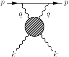
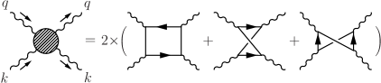
Figure 9.2: Feynman diagram of $e\gamma\to e\gamma$ scattering with LBL mechanism to be realized by quark-loops

Averaging over the initial electron and photon spin states (initial and final spin states are supposed to coincide) one can write down the amplitude of the process (9.47) in the following form

$$A^{e\gamma\to e\gamma}(s,t=0)=s\frac{\alpha}{4\pi^{2}}\int\frac{d^{2}\bf{q}}{(q^{2})^{2}}ds_{1}\sum_{\varepsilon}A^{\gamma\gamma\to\gamma\gamma}_{\mu\nu\alpha\beta}\frac{p^{\mu}p^{\nu}\varepsilon^{\alpha}\varepsilon^{*\beta}}{s^{2}},$$ (9.48)

where the light-cone projection of the light-by-light (LBL) scattering tensor takes the form

$$A^{\gamma\gamma\to\gamma\gamma}(s_{1},{\bf{q}})=A^{\gamma\gamma\to\gamma\gamma}_{\mu\nu\alpha\beta}\frac{p^{\mu}p^{\nu}\varepsilon^{\alpha}\varepsilon^{*\beta}}{s^{2}}=-\frac{8\alpha^{2}}{\pi^{2}}N_{c}Q^{4}_{q}\int d^{4}q_{-}\Big{[}\frac{S_{1}}{D_{1}}+\frac{S_{2}}{D_{2}}+\frac{S_{3}}{D_{3}}\Big{]}$$ (9.49)

with

$$\frac{S_{1}}{D_{1}}=\frac{(1/4)Tr\hat{p}(\hat{q}_{-}+m_{q})\hat{p}(\hat{q}_{-}-\hat{q}+m_{q})\hat{\varepsilon}^{*}(\hat{q}_{-}-\hat{q}+\hat{k}+m_{q})\hat{\varepsilon}(\hat{q}_{-}-\hat{q}+m_{q})}{(q_{-}^{2}-m^{2}_{q})((q_{-}-q)^{2}-m^{2}_{q})^{2}((q_{-}-q+k)^{2}-m^{2}_{q})},$$ (9.50)

$$\frac{S_{2}}{D_{2}}=\frac{(1/4)Tr\hat{p}(\hat{q}_{-}+m_{q})\hat{p}(\hat{q}_{-}-\hat{q}+m_{q})\hat{\varepsilon}^{(}\hat{q}_{-}-\hat{q}-\hat{k}+m_{q})\hat{\varepsilon}^{*}(\hat{q}_{-}-\hat{q}+m_{q})}{(q_{-}^{2}-m^{2}_{q})((q_{-}-q)^{2}-m^{2}_{q})^{2}((q_{-}-q-k)^{2}-m_{q}^{2})},$$ (9.51)

$$\frac{S_{3}}{D_{3}}=\frac{(1/4)Tr\hat{p}(\hat{q}_{-}+m_{q})\hat{\varepsilon}(\hat{q}_{-}-\hat{k}+m_{q})\hat{p}(\hat{q}_{-}+\hat{q}-\hat{k}+m_{q})\hat{\varepsilon}^{*}(\hat{q}_{-}+\hat{q}+m_{q})}{(q_{-}^{2}-m^{2}_{q})((q_{-}+q)^{2}-m^{2}_{q})((q_{-}+q+k)^{2}-m^{2}_{q})((q_{-}-k)^{2}-m^{2}_{q})}.$$ (9.52)

where $q_{-}$ means the quark four-momentum in the quark loop of the process $\gamma\gamma\to\gamma\gamma$, $N_{c}$ is the number of colors in QCD and $Q_{q}$ is the charge of the quark $q$ in electron charge units.

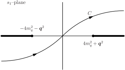
Figure 9.3: The path $C$ of an integration in (9.53)

Now, taking a derivative of the relation (9.48) according to $d^{2}{\bf{q}}$ and investigating the analytic properties of the obtained expression in the $s_{1}$-plane one gets the configuration as presented in Fig. 9.3, where also the path $C$ of the integral expression

$$I=\int_{C}ds_{1}\frac{dA^{e\gamma\to e\gamma}(s_{1},{\bf{q}})}{d^{2}{\bf{q}}}$$ (9.53)

is drawn. When the integration contour is closed to the right (on s-channel cut) and to the left (on the $u$-channel cut) one comes to the relation

$$\int^{-\infty}_{-4m^{2}_{q}-{\bf{q}^{2}}}ds_{1}\Delta_{u}\frac{dA^{e\gamma\to e\gamma}(s_{1},{\bf{q}})}{d^{2}{\bf{q}}}{|_{left}}=\int^{\infty}_{4m^{2}_{q}+{\bf{q}}^{2}}ds_{1}\Delta_{s}\frac{dA^{e\gamma\to e\gamma}(s_{1},{\bf{q}})}{d^{2}{\bf{q}}}{|_{right}},$$ (9.54)

where the right s-cannel discontinuity by means of Eq.(9.48) is related, due to optical theorem in a differential form

$$\Delta_{s}\frac{dA^{e\gamma\to e\gamma}(s,0)}{d^{2}{\bf{q}}}=2s\frac{d\sigma^{e\gamma\to eq\bar{q}}}{d^{2}{\bf{q}}},$$ (9.55)

to the $Q^{2}$=${\bf{q}}^{2}$=$-q^{2}$ dependent differential cross-section of $q\bar{q}$ pair creation by electron on photon, to be well known in the framework of QED [196] for $l^{+}l^{-}$ pair creation

$$\frac{4\alpha^{3}}{3(q^{2})^{2}}f(\frac{{\bf{q}}^{2}}{m^{2}_{q}})N_{c}Q^{4}_{q}=\frac{d\sigma^{e\gamma\to eq\bar{q}}}{d{\bf{q}}^{2}},$$ (9.56)

$$f(\frac{{\bf{q}}^{2}}{m^{2}_{q}})=({\bf{q}}^{2}-m^{2}_{q})J+1,$$

$$J=\frac{4}{\sqrt{{\bf{q}}^{2}({\bf{q}}^{2}+4m^{2}_{q})}}\ln[\sqrt{{\bf{q}}^{2}/(4m^{2}_{q})}+\sqrt{1+{\bf{q}}^{2}/(4m^{2}_{q})}].$$

But the right hand cut concerns of two real quark production for $s_{1}>4m_{q}^{2}$, which is associated wit 2 jets production.

The left-hand cut contribution has the same form as in QED case with constituent quark masses and as a result one obtains

$$\frac{4\alpha^{3}}{3({\bf{q}}^{2})^{2}}N_{c}\sum_{q}Q_{q}^{4}f(\frac{{\bf{q}}^{2}}{m_{q}^{2}})=\frac{d\sigma^{e\gamma\to e2jets}}{d{\bf{q}}^{2}}.$$ (9.57)

Finally, for the case of small ${\bf{q}}^{2}$ and applying the Weizsäcker-Williams relation, one comes to the sum rule for photon target [192] as follows

$$\frac{14}{3}\sum_{q}\frac{Q_{q}^{4}}{m_{q}^{2}}=\frac{1}{\pi\alpha^{2}}\int\limits_{4m^{2}_{q}}^{\infty}\frac{ds_{1}}{s_{1}}\sigma_{tot}^{\gamma\gamma\to 2{jet}}(s_{1}).$$ (9.58)

The quantity $\sigma_{tot}^{\gamma\gamma\to 2jets}(s_{1})$ is assumed to degrease for large values of $s_{1}$. It corresponds to the events in $\gamma\gamma$ collisions with creation of two jets, which are not separated by rapidity gaps and for which until the present days there is no experimental information. The latter complicates a verification of the obtained sum rule for photon target.

10 Conclusions

In this review we have formulated the main principles of a construction of the universal Unitary and Analytic model of the hadron electro-weak structure. Before the problem of inconsistency of the asymptotic behavior of VMD model with the asymptotic behavior of form factors of baryons and nuclei is solved, leading to a formulation of the asymptotic conditions and their general solutions giving explicitly all three possible forms of VMD form factor representations to be automatically normalized and possessing the right asymptotic behavior as required by the quark model of strongly interacting particles. Also a general approach for determination of the lowest normal and anomalous singularities of form factors from the corresponding Feynman diagrams is formulated. Finally, a number of concrete results to be obtained by making use of the analytic properties of the dynamical physical quantities, like electro-weak form factors of hadrons or amplitudes of various electromagnetic processes of hadrons is presented. Some of them are already successfully verified in practice, others are expecting for experimental confirmation. All this together demonstrates the analyticity to be an unavoidable powerful tool of the present particle physics phenomenology.

References

- [1] R. Hofstadter, F. Bumiller, M. R. Yearian, Rev. Mod. Phys. 30 (1958) 483.
- [2] J. J. Sakurai, Currents and Mesons, Univ. of Chicago Press, 1967.
- [3] V.A. Matveev, R.M. Muradyan and A.N. Tavkhelidze, Lett.Nuovo Cim. 7 (1973) 719.
- [4] S.J. Brodsky and G.R. Farrar, Phys.Rev.Lett. 31 (1973) 1153.
- [5] G.P. Lepage and S.J Brodsky, Phys.Lett. 87B (1979) 351.
- [6] G.R. Farrar and D.R. Jackson, Phys.Rev.Lett. 43 (1979) 246.
- [7] A.V. Efremov and A.V. Radyushkin, Phys.Lett. 94B (1980) 245.
- [8] M.A. Shifman, A.I. Vainshtein and V.I. Zakharov, Nucl.Phys. B147 (1979) 385.
- [9] V.A. Nesterenko and A.V. Radyushkin, Phys.Lett. 115B (1982) 410.
- [10] B.L. Ioffe and A.V. Smilga, Phys.Lett. 114B (1982) 353.
- [11] J. Gasser and H. Leutwyler, Nucl.Phys. B250 (1985) 517.
- [12] C. Amsler et al, Phys. Lett. B667 (2008) 1.
- [13] C. Adamuscin, A.Z. Dubnickova, S. Dubnicka, R. Pekarik, P. Weisenpacher, Eur. Phys. J. C28 (2003) 115.
- [14] S. Dubnicka, A.Z. Dubnickova, P. Weisenpacher, Eur. Phys. J. C32 (2004) 381.
- [15] S.S. Schweber: An introduction to relativistic quantum firld theory, Row - Peterson and Co, Evanston (Ill.), Elmsford, N.Y. 1961.
- [16] L.D. Landau, Nucl. Phys. 13 (1959) 181.
- [17] R. Eden, P. Landshoff, D. Olive, J. Polkinghorn: The analytic S-matrix, Cambridge Univ. Press, Cambridge (UK) 1966.
- [18] S. Dubnicka, O. Dumbrajs, Phys. Reports 19C (1975) 141.
- [19] R.E. Cutkosky, J. Math. Phys. 1 (1960) 429.
- [20] R. Oehme, Newsletter 7 (1992) 1.
- [21] B.R. Martin, D. Morgan and G. Shaw: Pion-Pion Interactions in Particle Physics; Academic Press, London-New York-San Francisco, 1976.
- [22] P. Estabrooks and A.D. Martin, Nucl. Phys. B79 (1974) 301.
- [23] B. Hyams et al, Nucl. Phys. B64 (1973) 134.
- [24] S.D. Protopopescu et al, Phys. Rev. D7 (1973) 1279.
- [25] S.J. Brodsky, Springer Tracts Mod. Phys. 100 (1982) 81.
- [26] M.K. Chose, Nucl. Phys. B174 (1980) 109.
- [27] V.L. Auslender et al, Sov. J. Nucl. Phys. 9 (1969) 69.
- [28] D. Benaksas et al, Phys. Lett. 39B (1972) 289.
- [29] E.B. Dally et al, Phys. Rev. Lett. 48 (1982) 375.
- [30] S.R. Amendolia et al, Nucl. Phys. B277 (1986) 168.
- [31] C.J. Bebek et al, Phys. Rev. D17 (1978) 1693.
- [32] J. Volmer et al, Phys. Rev. Lett. 86 (2001) 1713.
- [33] T. Horn et al, Phys. Rev. Lett. 97 (2006) 192001.
- [34] S.F. Berezhnev et al, Sov. J. Nucl. Phys. 18 (1973) 53.
- [35] S.F. Berezhnev et al, Sov. J. Nucl. Phys. 26 (1977) 290.
- [36] V.V. Alidze et al, Sov. J. Nucl. Phys. 33 (1981) 189.
- [37] A.Z. Dubnickova, S. Dubnicka, M.P. Rekalo, Z. Phys. C70 (1996) 473.
- [38] A. Quenzer et al, Phys. Lett. 76B (1978) 512.
- [39] G. Cosme et al, Preprint LAL-1287, ORSAY (1976).
- [40] D. Bisello et al, Phys. Lett. 220B (1989) 321.
- [41] D. Bollini et al, Lett. Nuovo Cim. 14 (1975) 418.
- [42] B. Esposito et al, Lett. Nuovo Cim. 28 (1980) 337.
- [43] A. Aloisio et al, Phys. Lett. B606 (2005) 12.
- [44] L.M. Barkov et al, Nucl. Phys. B256 (1985) 365.
- [45] R.R. Akhmetshin et al, Phys. Lett. B648 (2007) 28.
- [46] M.N. Achasov et al, JETP Vol.103 No.3 (2006) 380.
- [47] S.R. Amendolia et al, Phys. Lett. 138B (1984) 454.
- [48] R.M. Baltrusaitis et al, Phys. Rev. D32 (1985) 566.
- [49] S. Dubnicka, L. Martinovic, Czech. J. Phys. B29 (1979) 1384.
- [50] S. Dubnicka, V.A. Meshcheryakov and J. Milko, J. Phys. G7 (1981) 605.
- [51] S. Dubnicka, L. Martinovic, Lett. Nuovo Cim. 44 No.7 (1985) 462.
- [52] S. Dubnicka, L. Martinovic: Proc. XXI. Recontre de Moriond : Strong Interactions and Gauge Theories, March 16-22, 1986, Ed.: J. Tran Thanh Van, Frontiéres, Gif sur Yvette (1986) p. 297.
- [53] M.E. Biagini, S. Dubnicka, E. Etim, P. Kolar, Nuovo Cim. A104 (1991) 363.
- [54] E.B. Dally et al, Phys. Rev. Lett. 45 (1980) 232.
- [55] S.R.Amendolia et al, Phys. Lett. 178B (1986) 435.
- [56] S. Dubnicka, Preprint JINR, E2-88-840, Dubna (1988).
- [57] S.S. Gerstein, Ya.B. Zeldovich, ZhETP 29 (1955) 698.
- [58] R.P. Feynman, M. Gell-Mann, Phys. Rev. 109 (1958) 193.
- [59] Y. Nambu, Phys. Rev. 106 (1957) 1366.
- [60] A.Z. Dubnickova, S. Dubnicka, M.P. Rekalo, Czech. J. Phys. 43 (1993) 1057.
- [61] A.Z. Dubnickova, S. Dubnicka, M.P. Rekalo, Acta Phys. Univ. Com. XL (1999) 17.
- [62] D. Buskulic et al, Z. Phys. C70 (1996) 579.
- [63] M. Fujikawa et al., Phys. Rev. D78 (2008) 072006.
- [64] E. Bartos, S. Dubnicka, A.Z. Dubnickova, M. Fujikawa, H. Hayashii, Nucl. Phys. B (Proc. Suppl.) 198 (2010) 186.
- [65] S. Schael et al., Phys. Rept. 421 (2005) 191.
- [66] S. Anderson et al., Phys. Rev. D61 (2000) 112002.
- [67] D. Bisello et al, Z. Phys. C48 (1990) 23.
- [68] S. Dubnicka, Nuovo Cim. A100 (1988) 1.
- [69] R. C. Walker et al., Phys. Rev D49 (1994) 5671.
- [70] L. Andivahis et al., Phys. Rev. D50 (1994) 5491.
- [71] A. F. Sill et al., Phys. Rev. D48 (1993) 29.
- [72] A. Lung et al., Phys. Rev. Lett. 70 (1993) 718.
- [73] S. Rock et al., Phys. Rev. D46 (1992) 24.
- [74] P. Markowitz et al., Phys. Rev. C48 (1993) 5.
- [75] E. E. Bruins et al., Phys. Rev. Lett. 75 (1995) 21.
- [76] M. Mayerhoff et al., Phys. Lett. 327B (1994) 201.
- [77] S. Platchkov et al., Nucl. Phys. A510 (1990) 740.
- [78] T. Eden et al., Phys. Rev. C50 (1994) R1749.
- [79] M. Ostrick et al., Phys. Rev. Lett. 83 (1999) 276.
- [80] C. Herberg et al., Eur. Phys. J. A5 (1999) 131.
- [81] J. Becker et al., Eur. Phys. J. A6 (1999) 329.
- [82] D. Rohe et al., Phys. Rev. Lett. 83 (1999) 4257.
- [83] I. Passchier et al., Phys. Rev. Lett. 82 (1999) 4988.
- [84] G. Bassompierre et al, Nuovo Cimento A73 (1983) 347.
- [85] B. Delcourt et al, Phys. Lett. 86B (1979) 395.
- [86] D. Bisello et al, Nucl. Phys. B224 (1893) 379.
- [87] T.A. Armstrong et al, Phys. Rev. Lett. 70 (1993) 1212.
- [88] M. Ambrogioni et al, FNAL PUB-99/027-E, Batavia (1999).
- [89] D. Bisello et al, J. Phys. C48 (1990) 23.
- [90] G. Bardin et al, Nucl. Phys. B411 (1994) 3.
- [91] A. Antonelli et al, Phys. Lett. 334B (1994) 431.
- [92] C. Voci, Nucl. Phys. A623 (1997) 333c.
- [93] P. Mergell, U.-G. Meissner and D. Drechsel, Nucl. Phys. A596 (1996) 367.
- [94] S. Furuichi and D. Watanabe, Nuovo Cimento A110 (1997) 577.
- [95] H.-W. Hammer, Ulf-G. Meissner and D. Drechsel, Phys. Lett. 385B (1996) 343.
- [96] G. Höhler et al, Nucl. Phys. B114 (1976) 505.
- [97] S.Dubnicka, A.Z.Dubnickova and P.Weisenpacher, J. Phys. G 29 (2003) 405.
- [98] G. Höhler and E. Pietarinen, Phys. Lett. 53B (1975) 471.
- [99] S. J. Brodsky and P. G. Lepage, Phys. Rev. D22 (1980) 2157.
- [100] T.Frederico, H.-Ch.Pauli and Shan-Sui Zhan, Phys. Rev. D66 (2002) 116011.
- [101] M. K. Jones et al, Phys. Rev. Lett. 84 (2000) 1398.
- [102] O. Gayon et al, Phys. Rev. Lett. 88 (2002) 092301.
- [103] V. Punjabi et al, Phys. Rev. C71 (2005) 055202.
- [104] C. Adamuscin, S. Dubnicka, A.Z. Dubnickova, P. Weisenpacher, Prog. Part. Nucl. Phys. 55 (2005) 228.
- [105] E. Bartoš, S. Dubnička, E. A. Kuraev, Phys. Rev. D70 (2004) 117901.
- [106] R. A. Gilman and F. Gross, J. Phys. G28 (2002) R37.
- [107] V.M. Muzafarov et al, Sov. J. Part. Nucl. 14 (1983) 467.
- [108] R. Dymarz, F.C. Khanna, Phys. Rev. C41 (1990) 2438.
- [109] L.L. Frankfurt and M.I. Strikman, Phys. Rep. 76C (1981) 215.
- [110] T.S. Cheng and L.S. Kisslinger, Phys. Rev. C35 (1987) 1432.
- [111] E. Braaten and L. Carlson, Phys. Rev. D39 (1989) 838.
- [112] C. Adamuscin, S. Dubnicka, A.Z. Dubnickova, to be published
- [113] S.J. Brodsky and J.R. Hiller, Phys. Rev. D46 (1992) 2141.
- [114] S.J. Brodsky, C.-R. Ji and G.P. Lepage, Phys. Rev. Lett. 51 (1983) 83.
- [115] C.E. Carlson and F. Gross, Phys. Rev. D36 (1987) 2060.
- [116] A.Z. Dubnickova and S. Dubnicka, ICTP Trieste Report No.IC/91/149, 1991.
- [117] M. Garcon and J.W. Van Orden, Adv. Nucl. Phys. 26 (2001) 293.
- [118] B. Grossetete, B .Drickey and P. Lehman, Phys. Rev. 141 (1966) 1425.
- [119] J.E. Elias et al, Phys.Rev. 177 (1969) 2075.
- [120] S. Galster et al. Nucl.Phys. B32 (1971) 221.
- [121] R.W. Berard at al., Phys. Lett. B47 (1973) 355.
- [122] G.G. Simon et al., Nucl.Phys. A364 (1981) 295.
- [123] R. Cramer et al., Z. Phys. C29 (1985) 513.
- [124] L.C. Alexa et al., Phys.Rev. Lett. 82 (1999) 1374.
- [125] D. Abbott et al., Phys. Rev.Lett. 82 (1999) 1379.
- [126] C.D. Buckanan and R. Yerian, Phys. Rev. Lett. 15 (1965) 303.
- [127] R.E. Rand et al, Phys. Rev. lett. 18 (1967) 469.
- [128] D. Ganichot et al., Nucl.Phys. A178 (1972) 542.
- [129] G.G. Simon et al, Nucl.Phys. A364 (1981) 285.
- [130] R. Cramer et al., Z. Phys. C29 (1985) 513.
- [131] S. Aufret et al, Phys.Rev. Lett. 54 (1985) 649.
- [132] R.G. Arndd et al, Phys.Rev. Lett. 58 (1987) 1723.
- [133] P.E. Bosted et al, Phys. Rev. C42 (1990) 38.
- [134] M.E. Schulze et al, Phys. Rev. Lett. 52 (1984) 597.
- [135] V.F. Dmitrev et al, Phys. Lett. B157 (1985) 143.
- [136] B.B. Wojtsehkowski et al, JETP Lett. 43 (1986) 733.
- [137] R. Gilman et al., Phys. Rev. Lett. 65 (1990) 1723.
- [138] I. The et al, Phys. Rev. Lett. 67 (1991) 173.
- [139] M. Garcon et al, Phys. Rev. C49 (1994) 251.
- [140] M. Fero-Luzzi et al, Phys. Rev. Lett. 77 (1996) 2630.
- [141] M. Bouwhuis et al., Phys. Rev. Lett. 82 (1999) 3755.
- [142] D. Abbott et al., Phys. Rev. Lett. 84 (2000) 5053.
- [143] D.M. Nikolenko et al., Nucl.Phys. A684 (2001) 525c.
- [144] http://root.cern.ch
- [145] P.A.M. Guichon and M. Vanderhaeghen, Phys. Rev. Lett. 91 (2003) 142303.
- [146] P.G. Blunden, W. Melnitchouk and J.A. Tjon, Phys. Rev. C72 (2005) 034612.
- [147] A. V. Afanasiev, S. J. Brodsky, C. E. Carlson, Y. C. Chen and M. Vanderhaeghen, Phys. Rev. D72 (2005) 013008.
- [148] C. Adamuscin, L. Bimbot, S. Dubnicka, A.Z. Dubnickova, Phys. Rev. C78 (2008) 025202-1
- [149] M. Lacombe, B. Loiseau, J. M. Richard, R. Vinh Mau, J. Cote, P. Pires and R. De Tourreil, Phys. Rev. C21 (1980) 861.
- [150] S. Dubnicka, A.Z. Dubnickova, Prog. Part. Nucl. Phys. 61 (2008) 198.
- [151] R.L. Jaffe, Phys. Lett. B229 (1989) 275.
- [152] B.Mueller et al.[SAMPLE Collab.], Phys. Rev. Lett. 78 (1997) 3824.
- [153] F.E. Maas et al.[A4 Collab.], Phys. Rev. Lett. 93 (2004) 022002.
- [154] D.T. Spayde et al.[SAMPLE Collab.], Phys. Lett. B583 (2004) 79.
- [155] D.S. Armstrong et al.[G0 Collab.], Phys. Rev. Lett. 95 (2005) 092001.
- [156] F. E.Maas et al.[A4 Collab.], Phys. Rev. Lett. 94 (2005) 152001.
- [157] S. Dubnicka, A.Z. Dubnickova, J. Phys. G28 (2002) 2137.
- [158] A.I. Akhiezer and M.P. Rekalo, Sov. Phys. Dokl. 13 (1968) 572.
- [159] A.Z. Dubničková, S. Dubnička, M.P. Rekalo, Nuovo Cim. A109 (1996) 241.
- [160] A.Z. Dubnickova, S. Dubnicka, M. Erdelyi, Prog. Part. Nucl. Phys. 61 (2008) 162.
- [161] G.I. Gakh, E. Tomasi-Gustafsson, C. Adamuscin, S. Dubnicka, A.Z. Dubnickova, Phys. Rev. C74 (2006) 025202-1.
- [162] C. Adamuscin, S. Dubnicka, A.Z. Dubnickova, Phys. Rev. C80 (2009) 018202-1.
- [163] G.W. Bennett et al., Phys. Rev. Lett. 89 (2002) 101804-1.
- [164] V. W. Hughes and T. Kinoshita, Rev. Mod. Phys. 71 (2) (1999) S133.
- [165] A. Czarnecki, W. Marciano, Nucl. Phys. B(Proc. Suppl.) 76 (1999) 245.
- [166] G. Degrassi and G. F. Giudice, Phys. Rev. D58 (1998) 53007.
- [167] M. Knecht, S. Peris, M. Perrottet, E. de Rafael, hep-ph/0205102.
- [168] T. Kinoshita et al., Phys. Rev. D31 (1985) 2108.
- [169] J.A. Casas et al., Phys. Rev. D32 (1985) 736.
- [170] L. Martinovic and S. Dubnicka, Phys. Rev. D 42 (1990) 884.
- [171] S. Eidelman, F. Jegerlehner, Z. Phys. C67 (1995) 585.
- [172] S. Narison, Phys. Lett. 513 B (2001) 53.
- [173] E. Bartos, A.Z. Dubnicková, S. Dubnicka, E.A. Kuraev, E. Zemlyanaya, Nucl. Phys. B632 (2002) 330.
- [174] M. Hyakawa, T. Kinoshita, hep-ph/0112102.
- [175] J. Bijnens et al., hep-ph/0112255.
- [176] M. Knecht and A. Nyffeler, hep-ph/0111058.
- [177] I. Blokland, A. Czarnecki and K. Melnikov, hep-ph/0112117.
- [178] S. Dubnicka, G. Georgios, V.A. Meshcheryakov, Can. J. Phys. 63 (1985) 1357.
- [179] M. Nagy, M. K. Volkov and V. L. Yudichev, Proc. of Int. Conf. ”Hadron Structure 2000”, Stara Lesna, Slovak Republic, 2.-7.10. 2000, Eds: A.-Z. Dubnickova, S. Dubnicka and P. Strizenec, Comenius Univ., Bratislava (2001) p. 188.
- [180] E.M. Aitala et al., Phys. Rev. Lett. 86 (2001) 70.
- [181] T. Komada, M. Ishida and S. Ishida, Phys. Lett. 508 B (2001) 31.
- [182] B. Krause, Phys. Lett. 390 B (1997) 392.
- [183] M. Davier, Nucl. Phys. B (Proc. Suppl.) 169 (2007) 288.
- [184] K. Hagiwara, A. D. Martin, D. Nomura and T. Teubner, Phys. Lett. B649 (2007) 173.
- [185] J. F. de Troconiz and F. J. Yndurain, Phys. Rev. D71 (2005) 073008.
- [186] E. Bartos, S. Dubnicka, A.Z. Dubnickova, A. Liptaj, Nucl. Phys. B. (Proc. Suppl.) 198 (2010) 194.
- [187] V.De Alfaro, S.Fubini, G.Furlan and C.Rosetti: Currents in hadron physics, American Elsevier Publ. Company, Inc., New York (1973).
- [188] K.Gottfried, Phys. Rev. Lett. 18 (1967) 1174.
- [189] E.Kuraev, M.Secansky and E.Tomasi-Gustafsson, Phys. Rev. D73 (2006) 125016-1.
- [190] S.Dubnicka, A.Z.Dubnickova and E.A.Kuraev, Phys. Rev. D75 (2007) 057901-1.
- [191] S.Dubnicka, A.Z.Dubnickova and E.A.Kuraev, Phys. Rev. D74 (2006) 034023-1.
- [192] E.Bartos, S.Dubnicka, A.Z.Dubnickova and E.A.Kuraev, Phys. Rev. D76 (2007) 057901-1.
- [193] V.N.Baier, V.S.Fadin, V.A.Khose and E.A.Kuraev, Phys. Rep. 78 (1981) 293.
- [194] N.Cabibbo and L.A.Radicati, Phys. Lett. 19 (1966) 697.
- [195] B.Kubis and U.-G.Meissner, Eur. Phys. J. C18 (2001) 747.
- [196] S.R.Kel’ner, Yad. Fiz. 5 (1967) 1092.