Inanotech/LMS/09/04
Electronic Properties and Hidden Symmetries of Graphene

Abstract

Using the relation between the structural and the electronic properties of honeycomb, we study the hidden $SU\left(3\right)$ symmetry of the graphene monolayer and exhibit the link with its electronic properties. We show that the conservation law of incoming and outgoing electronic momenta at each site of graphene is solved in terms of SU$\left(3\right)$ representations; and the Fourier waves $\tilde{\phi}\left(k_{x},k_{y}\right)$ of the hopping electron may be classified by SU$\left(3\right)$ highest weight multiplets $\phi_{p,q}\left(\xi\right)$. It is also shown that the phases $\arctan\frac{k_{y}}{k_{x}}$ of the waves are quantized as $\frac{\left(p+q\right)}{\left(p-q\right)}\sqrt{3}$ with $p,$ $q$ positive integers. Other features are also discussed.

1 Introduction

Graphene is a system of carbon atoms in the sp² hybridization forming a 2D honeycomb lattice. This is a planar system made of two triangular sublattices A and B and constitute the building block of graphite. Since its experimental realization in 2004, the study of the electronic properties of graphene with and without external fields has been a big subject of interest [1]-[4]; some of its main physical aspects were recently reviewed in [5] and refs therein. This big interest into graphene and its derivatives is because they offer a real alternative for silicon based technology and bring together issues from condensed matter and high energy physics [6]-[12] allowing a better understanding of the electronic band structure as well as their special properties.
In this paper, we focus on an unexplored issue of 2D graphene by studying the link between specific electronic properties and a class of hidden symmetries of the honeycomb. These symmetries allow to get more insight in the transport property of the electronic wave modes and may be used to approach the defects and boundaries [13]. The existence of these hidden symmetries; in particular of the remarkable hidden $SU\left(3\right)$ invariance considered in this study, may be motivated from several views. For instance from the structure of the first nearest carbon neighbors like for the typical $\left\langle A_{0}\text{-}B_{1}\right\rangle$, $\left\langle A_{0}\text{-}B_{2}\right\rangle,$ $\left\langle A_{0}\text{-}B_{3}\right\rangle$ see fig(1) for illustration and more details.

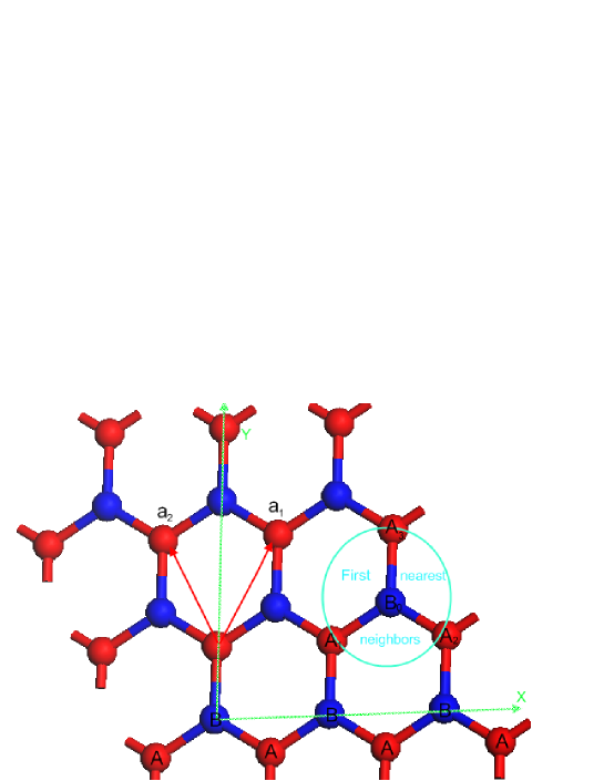
Figure 1: Sublattices $\mathcal{A}$ and $\mathcal{B}$ of the honeycomb. A-type carbons are given by red balls and B-type atoms by blue ones. Each carbon has 3 first nearest neighbors and 6 second nearest ones.

These are basic patterns generating three $SU\left(2\right)$ symmetries contained in the hidden SU$\left(3\right)$ invariance of honeycomb. The $\left\langle A\text{-}B\right\rangle$ patterns transform in the isospin $\frac{1}{2}$ representations and describe the electronic wave doublets $\phi_{{\scriptsize\pm}\frac{{\scriptsize 1}}{{\scriptsize 2}}}=\left[a\left(\mathbf{r}\right),b\left(\mathbf{r}\right)\right]$ interpreted as quasi-relativistic 2D spinors in the nearby of the Dirac points [5]. The $SU\left(3\right)$ hidden symmetry of honeycomb is also encoded in the second nearest neighbors $\left\langle\left\langle A_{0}\text{-}A_{i}\right\rangle\right\rangle$ and $\left\langle\left\langle B_{0}\text{-}B_{i}\right\rangle\right\rangle$, $i=1,...,6$, which capture information on its adjoint representation where the six $\left\langle\left\langle A_{0}\text{-}A_{i}\right\rangle\right\rangle$ (and similarly for $\left\langle\left\langle B_{0}\text{-}B_{i}\right\rangle\right\rangle$) are associated with the six roots of $SU\left(3\right)$. In addition to above mentioned properties, hidden symmetries of graphene are also present in the framework of the tight binding model with hamiltonian,

$$H=$$

,

where the fermionic creation and annihilation operators $a,$ $a^{\dagger},$ $b,$ $b^{\dagger}$ are respectively associated to the pi-electrons of each atom of the sublattices A and B and where the three relative vectors $\mathbf{\delta}_{1}$, $\mathbf{\delta}_{2}$, $\mathbf{\delta}_{3}$ define the first nearest neighbors as depicted in fig(1). These 2D vectors are globally defined on the honeycomb and obey the remarkable constraint equation $\mathbf{\delta}_{1}+\mathbf{\delta}_{2}+\mathbf{\delta}_{3}=\mathbf{0}$ which, a priori, encodes also information on the electronic properties of graphene. Throughout this study, we show amongst others, that the three above mentioned $SU\left(2\right)$’s are intimately related with these $\mathbf{\delta}_{n}$’s which, as we will see, are nothing but roots of $SU\left(3\right)$. We also show that the mapping of the condition $\sum_{n=1}^{3}\mathbf{\delta}_{n}=\mathbf{0}$ to the momentum space can be interpreted as a condition on the conservation of total momenta at each site of honeycomb whose solutions are classified by highest weight state representations of the $SU\left(3\right)$ symmetry. We show moreover that the hamiltonian $H$ of the tight binding model for first nearest neighbors has an interpretation in terms of the $F^{\pm\beta}$ step operators of these $SU\left(2\right)$’s opening a window for more insight into the study of the electronic correlations in graphene and cousin systems.
The organization of this paper is as follows: In section 2, we exhibit the $SU\left(3\right)$ symmetry of graphene. In section 3, we give a field theoretic interpretation of the geometric constraint equation $\mathbf{\delta}_{1}+\mathbf{\delta}_{2}+\mathbf{\delta}_{3}=\mathbf{0}$ both in real and reciprocal honeycomb. We also use the roots and weights of hidden $SU\left(3\right)$ symmetry to study aspects of the electronic properties of graphene. In section 4, we develop the relation between the energy dispersion and the hidden symmetries. In section 5, we give the conclusion and a perspective.

2 Hidden symmetries of graphene

In dealing with ideal 2D graphene, one notices the existence of a hidden $SU\left(3\right)$ group symmetry underlying the crystallographic structure of the honeycomb lattice and governing the hopping of the pi-electrons between the closed neighboring carbons. To exhibit this hidden $SU\left(3\right)$ symmetry, let us start by examining some remarkable features on the graphene lattice and show how they are closely related to SU$\left(3\right)$.
Refereing to the two sublattices of the graphene monolayer by the usual letters A and B generated by the vectors $\mathbf{a}_{1,2}=\frac{a}{2}(\pm\sqrt{3},3)$ and the relative ones $\mathbf{\delta}_{1,2}=\frac{a}{2}\left(\pm\sqrt{3},1\right)$, and denoting by $\phi_{A}\left(\mathbf{r}_{i}\right)$ and $\phi_{B}\left(\mathbf{r}_{j}\right)$ the wave functions of the corresponding pi-electrons, one notes that the interactions between the first nearest atoms involve two kinds of trivalent vertices capturing data on $SU\left(3\right)$ symmetry, see fig(2) for illustration.

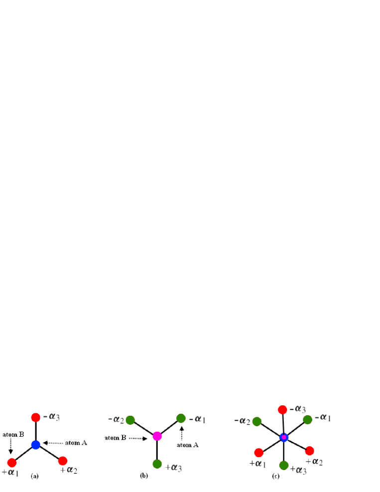
Figure 2:  (a) Nearest neighbors of a A- type atom. (b) Nearest neighbors of a B-type atom. (c) The fusion of the two vertices gives the adjoint representation of SU$\left({\small 3}\right)$.

This hidden $SU\left(3\right)$ invariance can be made more explicit by remarking that the relative vectors $\mathbf{\delta}_{1},$ $\mathbf{\delta}_{2}$ and $\mathbf{\delta}_{3}=-\mathbf{\delta}_{1}-\mathbf{\delta}_{2}$ describing the three first closed neighbors to a A- type carbon at site $\mathbf{r}_{i}$ of the honeycomb together with their opposites $-\mathbf{\delta}_{n}$ for B-type carbons are precisely the roots of the $SU\left(3\right)$ algebra. Indeed, if forgetting about the scale dimension and thinking about the carbon-carbon distance $a\simeq 1.42$ $A^{{{}^{\circ}}}$ as the irrational number $a=\sqrt{2}$, one gets the remarkable identification

$$\mathbf{\delta}_{1}=\mathbf{\alpha}_{1}$$ , , ,

(2.1)

with $\mathbf{\alpha}_{1}$ and $\mathbf{\alpha}_{2}$ being the two simple roots of $SU\left(3\right)$. This symmetry can be also exhibited by computing the intersection matrix $\mathbf{\delta}_{i}\cdot\mathbf{\delta}_{j}$ of the two generators $\mathbf{\delta}_{1}$ and $\mathbf{\delta}_{2}$,

$$\mathbf{\delta}_{i}\cdot\mathbf{\delta}_{j}=\frac{a^{2}}{2}\left(\begin{array}[]{cc}2&-1\\ -1&2\end{array}\right),$$ (2.2)

which turns out to be proportional to the Cartan matrix of the $SU\left(3\right)$ algebra, $A_{ij}=\mathbf{\alpha}_{i}\cdot\mathbf{\alpha}_{j}$. Recall that the Lie algebra of SU$\left(3\right)$ has rank two, eight generators $\left\{F^{a}\right\}$ and commutation relations that read in the Gell-Mann basis like

$$\left[F^{a},F^{b}\right]=if^{abc}F^{c},$$ (2.3)

with antisymmetric structure constants as $f_{123}=1$, $f^{147}=f^{516}=f^{246}=f^{257}=f^{345}=f^{637}=\frac{1}{2}$ and $f^{458}=f^{678}=1$. In the Cartan-Weyl basis, useful for physical interpretations, we take $h^{1}=\sqrt{2}F^{8}$ and $h^{2}=\sqrt{2}F^{3}$ as the two Cartan terms and the six step operators like $\sqrt{2}U_{3}^{\pm}=F^{1}\pm iF^{2}$, $\sqrt{2}U_{2}^{\pm}=F^{4}\pm iF^{5}$, $\sqrt{2}U_{1}^{\pm}=F^{6}\pm iF^{7}$. The new commutation relations following from (2.3) read as follows,

$$\left[h^{i},U_{n}^{\pm}\right]=\pm\delta_{n}^{i}$$ ,

(2.4)

with $i=1,2$ and where the $\mathbf{\delta}_{n}$’s are the same vectors as in the graphene. Notice in passing that the hidden SU$\left(3\right)$ described above seems to be just a sub-symmetry of a larger one since the $\mathbf{\delta}_{n}$’s obey the constraint relation

$$\sum_{n=1}^{3}\mathbf{\delta}_{n}=\mathbf{0.}$$ (2.5)

which might hide an affine $S\hat{U}\left(3\right)$ Kac-Moody symmetry [14, 15] since the intersection matrix of the three relative $\mathbf{\delta}_{i}$- vectors reads as $\mathbf{\delta}_{i}\cdot\mathbf{\delta}_{j}=\frac{a^{2}}{2}\hat{A}_{ij}$ with

$$\hat{A}_{ij}=\left(\begin{array}[]{ccc}2&-1&-1\\ -1&2&-1\\ -1&-1&2\end{array}\right)$$ ,

(2.6)

describing exactly the generalized Cartan matrix of affine $S\hat{U}\left(3\right)$. Below, we shall restrict our study to the hidden ordinary $SU\left(3\right)$ symmetry of the graphene and think about (2.5) as a physical constraint equation governing the electronic properties of the graphene.

3 Electronic properties and $SU\left(3\right)$ symmetry

Quantum mechanically, there are two approaches to deal with the geometrical constraint relation (2.5). The first one is to work in real space and think about it as the conservation law of total space-time probability current densities at each site $\mathbf{r}_{i}$ of the honeycomb. The second approach relies on moving to the dual space where this constraint relation and the induced electronic properties get a remarkable interpretation in terms of $SU\left(3\right)$ representations.

3.1 Conservation of total current density

In the real space, the way we interpret eq(2.5) is in terms of the relation between the time variation of the probability density $\rho\left(t,\mathbf{r}_{i}\right)=\left|\phi\left(t,\mathbf{r}_{i}\right)\right|^{2}$ of the electron at site $\mathbf{r}_{i}$ and the sum

$$\sum_{n=1}^{3}\mathbf{J}_{{\scriptsize\delta}_{n}}\left(t,\mathbf{r}_{i}\right)=\mathbf{J}\left(t,\mathbf{r}_{i}\right)\text{ \ \ \ ,}$$ (3.1)

of incoming and outgoing probability current densities along the $\delta_{n}$- directions. On one hand, because of the equiprobability in hopping from the carbon at $\mathbf{r}_{i}$ to each one of the three nearest carbons at $\mathbf{r}_{i}+\mathbf{\delta}_{n}$, the norm of the $\mathbf{J}_{{\scriptsize\delta}_{n}}$- vector current densities should be equal and so they should have the form

$$\mathbf{J}_{{\scriptsize\delta}_{n}}\left(t,\mathbf{r}_{i}\right)=j\left(t,\mathbf{r}_{i}\right)\mathbf{e}_{n}$$ , .

(3.2)

These probability current densities together with the unit vectors $\mathbf{e}_{n}=\frac{\mathbf{\delta}_{n}}{a}$ point in the different $\mathbf{\delta}_{n}$- direction; but have the same non zero norm: $\left\|\mathbf{J}_{{\scriptsize\delta}_{1}}\right\|=\left\|\mathbf{J}_{{\scriptsize\delta}_{2}}\right\|=\left\|\mathbf{J}_{{\scriptsize\delta}_{3}}\right\|=\left|j\right|$. Substituting in the above relation, the total probability current density $\mathbf{J}\left(t,\mathbf{r}_{i}\right)$ at the site $\mathbf{r}$ and time $t$ takes then the factorized form

$$\mathbf{J}\left(t,\mathbf{r}\right)=\frac{j\left(t,r\right)}{a}\left(\sum_{n}\mathbf{\delta}_{n}\right).$$ (3.3)

On the other hand, by using the Schrodinger equation $i\hbar\frac{\partial\phi}{\partial t}=\left(-\frac{\hbar^{2}}{2m}\nabla^{2}+V\right)\phi$ describing the interacting dynamics of the electronic wave at $\mathbf{r}$, we have the usual conservation equation,

$$\frac{\partial\rho\left(t,\mathbf{r}\right)}{\partial t}+\mathop{\mathrm{d}iv}\mathbf{J}\left(t,\mathbf{r}\right)=0\text{ \ \ },$$ (3.4)

with probability density $\rho\left(t,\mathbf{r}\right)$ as before and $J=\frac{i\hbar}{2m}\left(\phi\nabla\phi^{\ast}-\phi^{\ast}\nabla\phi\right)$ with m the mass of the electron and $\phi=\phi\left(t,\mathbf{r}\right)$ its wave. Moreover, assuming $\frac{\partial\rho}{\partial t}=0$ corresponding to stationary electronic waves $\phi\left(t,\mathbf{r}\right)=e^{i\omega t}\phi\left(\mathbf{r}\right)$, it follows that the space divergence of the total current density vanishes identically; $\mathop{\mathrm{d}iv}\mathbf{J}=0$. This constraint equation shows that generally $\mathbf{J}$ should be a curl vector; but physical consideration indicates that we must have

$$\mathbf{J}\left(t,\mathbf{r}\right)=0\text{ \ \ ,}$$ (3.5)

in agreement with Gauss-Stokes theorem $\int_{\mathcal{V}}\mathop{\mathrm{d}iv}\mathbf{J}$ $d\mathcal{V}$ $\mathbf{=}$ $\int_{\partial\mathcal{V}}\mathbf{J.}d\mathbf{\sigma}$ leading to the same conclusion. Combining the property $\mathbf{J}\left(t,\mathbf{r}\right)=0$ with its factorized expression $\frac{j}{a}\left(\sum_{n}\mathbf{\delta}_{n}\right)$ given by eq(3.3) together with $j\neq 0$, we end with the constraint relation $\sum_{n}\mathbf{\delta}_{n}=0$.

3.2 Conservation of total phase

In the dual space of the electronic wave of graphene, the constraint relation (2.5) may be interpreted in two different, but equivalent, ways; first in terms of the conservation of the total relative phase $\Delta\varphi_{{\scriptsize tot}}=\sum\mathbf{k.}\Delta\mathbf{r}$ of the electronic waves induced by the hopping to the nearest neighbors. The second way is in terms of the conservation of the total momenta at each site of the honeycomb.
Decomposing the wave function $\phi\left(\mathbf{r}\right)$, associated with a A-type carbon at site $\mathbf{r}$, in Fourier modes as $\sum_{k}e^{i2\pi\mathbf{k}\cdot\mathbf{r}}$ $\tilde{\phi}\left(\mathbf{k}\right)$; and similarly for the B-type neighboring ones $\phi\left(\mathbf{r}+\mathbf{\delta}_{n}\right)=\sum_{k}e^{i2\pi\mathbf{k}\cdot\mathbf{r}}$ $\tilde{\phi}_{n}\left(\mathbf{k}\right)$ with $\mathbf{k=}\left(k_{x},k_{y}\right)$, we see that $\tilde{\phi}\left(k\right)$ and the three $\tilde{\phi}_{n}\left(k\right)$ are related as

$$\tilde{\phi}_{n}\left(k\right)=e^{i2\pi\theta_{n}}\tilde{\phi}\left(k\right)$$ ,  ,

(3.6)

with relative phases $\theta_{n}=\mathbf{k}\cdot\mathbf{\delta}_{n}$. These electronic waves have the same module, $\left|\tilde{\phi}_{n}\left(k\right)\right|^{2}=\left|\tilde{\phi}\left(k\right)\right|^{2}$; but in general non zero phases; $\theta_{1}\neq\theta_{2}\neq\theta_{3}$. This means that in the hop of an electron with momentum $\mathbf{p}=\hbar\mathbf{k}$ from a site $\mathbf{r}_{i}$ to the nearest at $\mathbf{r}_{i}+\mathbf{\delta}_{n}$, the electronic wave acquires an extra phase of an amount $\theta_{n}$; but the probability density at each site is invariant. Demanding the total relative phase to obey the natural condition,

$$\theta_{1}+\theta_{2}+\theta_{3}=0\text{ \ },\text{ \ \ }\mathop{\mathrm{m}od}\left(2\pi\right),$$ (3.7)

one ends with the constraint eq(2.5). Let us study two remarkable consequences of this special conservation law on the $\theta_{n}$ phases by help of the hidden $SU\left(3\right)$ symmetry of graphene.
(1) Using eq(2.1), which identifies the relatives $\mathbf{\delta}_{n}$ vectors with the roots $\mathbf{\alpha}_{n}$ of $SU\left(3\right)$ symmetry, as well as the Lie algebra duality relation

$$\mathbf{\alpha}_{i}\cdot\mathbf{\lambda}_{j}=\delta_{ij}$$ , ,

(3.8)

mapping the two simple roots $\mathbf{\alpha}_{1}$, $\mathbf{\alpha}_{2}$ into the $SU\left(3\right)$ fundamental weights $\mathbf{\lambda}_{1}$, $\mathbf{\lambda}_{2}$, we can invert the three equations $\theta_{n}=\mathbf{k}\cdot\mathbf{\delta}_{n}$ to get the $\mathbf{p}_{n}\mathbf{=}\hbar\mathbf{k}_{n}$ momenta of the electronic waves along the $\mathbf{\delta}_{n}$-directions.

Figure 3: Root/weight duality linking roots and weights $\mathbf{\alpha}_{i}\cdot\mathbf{\delta}_{j}=\delta_{ij}$.

For the two first $\theta_{n}$’s, that is $n=1,2$, the inverted relations are nicely obtained by decomposing the 2D wave vector $\mathbf{k}$ along the $\mathbf{\lambda}_{1}$ and $\mathbf{\lambda}_{2}$ directions of the dual lattice to end with the following particular solution,

$$\mathbf{k}_{1}=\theta_{1}\text{ }\mathbf{\lambda}_{1}$$ , .

(3.9)

More general solutions of type $\mathbf{k}_{1}=\theta_{1}$ $\mathbf{\lambda}_{1}+\varkappa_{2}$ $\mathbf{\lambda}_{2}$ and $\mathbf{k}_{2}=\varkappa_{1}$ $\mathbf{\lambda}_{1}+\theta_{2}$ $\mathbf{\lambda}_{2}$ will be considered in next subsection. Notice by the way that the 2D vectors $\mathbf{\lambda}_{1}$ and $\mathbf{\lambda}_{2}$, interpreted in the framework of SU$\left(3\right)$ group theory as the fundamental weights, are nothing but

$$\mathbf{\lambda}_{1}=\frac{1}{3}\mathbf{a}_{1}$$ , ,

(3.10)

where $\mathbf{a}_{1,2}=\frac{a}{2}(\pm\sqrt{3},3)$ stand for the generators of the A- type atoms introduced in the beginning of section 2; see also fig(1). The above relations (3.10) give an other evidence for the role of the SU$\left(3\right)$ symmetry in the study of the electronic properties of graphene.
(2) To get the wave vector from the relation $\theta_{3}=\mathbf{k}\cdot\mathbf{\delta}_{3}$, we decompose the 2D vector like $\mathbf{k}=q_{1}$ $\mathbf{\lambda}_{1}+q_{2}$ $\mathbf{\lambda}_{2}$; then substitute $\mathbf{\delta}_{3}=-\mathbf{\alpha}_{1}-\mathbf{\alpha}_{2}$ and use eq(3.8) to end with $\theta_{3}=-q_{1}-q_{2}$. Comparing with eq(3.7), we find that the wave vector $\mathbf{k}_{3}$ of the electronic wave along the $\mathbf{\delta}_{3}$- direction reads as follows,

$$\mathbf{k}_{3}=\theta_{1}\mathbf{\lambda}_{1}+\theta_{2}\mathbf{\lambda}_{2}\text{.}$$ (3.11)

Now, combining (3.9) and (3.11), we find that the property $\sum_{n}\theta_{n}=0$ describing the conservation law (3.7) of the total phase of the electron hops to nearest neighbors can be mapped to a constraint relation on the conservation of total outgoing and incoming momenta $\hbar\mathbf{k}_{n}$ at each site $\mathbf{r}_{i}$ of the honeycomb, i.e:

$$\mathbf{k}_{1}+\mathbf{k}_{2}-\mathbf{k}_{3}=\mathbf{0}$$ .

(3.12)

This result is not strange; it may be directly obtained by mapping (2.5) to the reciprocal lattice. Below, we study the solutions of this constraint relation in connection with the hidden $SU\left(3\right)$ symmetry of the honeycomb.

3.3 More on the constraint eq(3.12)

Seen that the relative vectors $\mathbf{\delta}_{n}$ defining the first nearest neighbors are roots of $SU\left(3\right)$ as shown by eq(2.1), a way to deal with the constraint relation (3.12) is to think about it as a $SU\left(3\right)$ group representation relation. This means that the wave vector in eq(3.11) may be thought of as given by $\mathbf{k}_{1}=\xi_{1}\mathbf{\Lambda}_{1}$, $\mathbf{k}_{2}=\xi_{2}\mathbf{\Lambda}_{2}$, $\mathbf{k}_{3}=\xi_{3}\mathbf{\Lambda}_{3}$ where the $\xi_{n}$’s are real numbers and $\mathbf{\Lambda}_{1}$, $\mathbf{\Lambda}_{2}$, $\mathbf{\Lambda}_{3}$ are three generic weight vectors of $SU\left(3\right)$. An interesting situation corresponds to the case where $\xi_{1}=\xi_{2}=\xi_{3}=\xi$ allowing to turn the constraint eq(3.12) into a constraint relation on $SU\left(3\right)$ weights,

$$\xi\left(\mathbf{\Lambda}_{1}+\mathbf{\Lambda}_{2}-\mathbf{\Lambda}_{3}\right)=\mathbf{0}$$ .

(3.13)

This is a remarkable relation which may be motivated by thinking about $SU\left(3\right)$ as a basic symmetry that governs the electronic properties in graphene. After all, eq(3.13) is the dual of (2.5) and moreover $\sum_{n=1}^{3}\mathbf{\delta}_{n}=\mathbf{0}$ is itself a $SU\left(3\right)$ condition; see also footnote 1. Under this hypothesis, and thinking about the $\mathbf{\Lambda}_{n}$’s as highest weight vectors that can be decomposed as,

$$\mathbf{\Lambda}_{n}=p_{n1}\mathbf{\lambda}_{1}+p_{n2}\mathbf{\lambda}_{2}$$ ,

(3.14)

we get, after substituting in (3.13), the following conditions on the $p_{ij}$ positive Dynkin integers,

$$\xi\left(p_{11}+p_{21}-p_{31}\right)=0$$ ,

.

(3.15)

The simplest solution of these relations corresponds to taking the weight vectors as

$$\mathbf{\Lambda}_{1}=\mathbf{\lambda}_{1}$$ , , ,

(3.16)

in agreement with eqs(3.9-3.11). Particular solutions type $\mathbf{\Lambda}=p\mathbf{\lambda}_{1}$ and $\mathbf{\Lambda}^{\prime}=p\mathbf{\lambda}_{2}$ with positive integer $p$ are in the same class as $\mathbf{\lambda}_{1}$ and $\mathbf{\lambda}_{2}$. From this analysis we learn that within the $SU\left(3\right)$ set up, the solutions of (3.12) have the following features:
(i) the norm of the wave vector of the $\tilde{\phi}\left(k_{n}\right)$ wave is $\mathbf{k}_{n}^{2}=\frac{2}{3}\left(p_{n1}^{2}+p_{n2}^{2}+p_{n1}p_{n2}\right)\xi^{2}$,
(ii) the phases of the waves $\tilde{\phi}_{n}\left(k_{x},k_{y}\right)$, defined by $\varphi_{n}=\arctan\left(\frac{k_{ny}}{k_{nx}}\right)$, are quantized as

$$\frac{k_{ny}}{k_{nx}}=\frac{\left(p_{n1}+p_{n2}\right)}{p_{n1}-p_{n2}}\sqrt{3}$$ .

(3.17)

(iii) the Fourier waves $\tilde{\phi}\left(k_{x},k_{y}\right)$ may be interpreted as 1D field multiplets transforming into $SU\left(3\right)$ highest weight representations as,

$$\tilde{\phi}\left(k_{x},k_{y}\right)=\tilde{\phi}_{\Lambda}\left(\xi\right)=\tilde{\phi}_{\left(p,q\right)}\left(\xi\right)$$ ,

(3.18)

with dimension

$$\frac{1}{2}\left(1+p\right)\left(1+q\right)\left(2+p+q\right)$$ .

(3.19)

In this $SU\left(3\right)$ picture, the physics describing the electron hops between the nearest carbons is completely captured by $SU\left(3\right)$ highest state representations. For instance, taking $\Lambda_{1}\equiv$ 3̱ and $\mathbf{\Lambda}_{2}\equiv\bar{3}$ as in fig(4), and using the tensor product decomposition

$$\text{\@text@baccent{3}}\otimes\bar{3}=9=\text{\@text@baccent{8}}\oplus\text{\@text@baccent{1}}$$ ,

(3.20)

the Fourier waves propagating between the nearest sites are $\tilde{\phi}_{\left(1,0\right)}$, $\tilde{\phi}_{\left(0,1\right)}$, $\tilde{\phi}_{\left(1,1\right)}$ and $\tilde{\phi}_{\left(0,0\right)}$. The zero mode $\tilde{\phi}_{\left(0,0\right)}$ describes the state where the electron doesn’t hop.

Figure 4: Real and dual lattices represented simultaneously. Total probability current density and total momenta of the electronic waves are conserved at each site of the honeycomb.

Notice that each of these $\phi_{\Lambda}\left(\xi\right)$ fields hide sub-modes $\left(\phi_{\mathbf{\lambda}}\right)^{\mu}$ associated with the various states of the representations. For the example of fig(4), we have:

$$\phi_{\mathbf{\lambda}}$$ , , ,

, , ,

, , ,

(3.21)

with $\mathbf{\lambda}^{{\scriptsize adj}}=\psi$. This degeneracy can be lifted by breaking down the hidden $SU\left(3\right)$ symmetry of the graphene. This may be achieved by implementing defects in the honeycomb that violate eq(3.15).

4 Energy dispersion and the hidden symmetries

The energy $h_{i}$ describing the hopping of a pi-electron from the site $\mathbf{r}_{i}$ to its three nearest neighbors at $\mathbf{r}_{i}+\mathbf{\delta}_{n}$ is nicely represented by the tight binding hamiltonian [16] whose total form reads as $H=-t\sum_{i}h_{i}$,

$$h_{i}=\sum_{n=0}^{2}a\left(\mathbf{r}_{i}\right)b^{\dagger}\left(\mathbf{r}_{i}+\mathbf{\alpha}_{n}\right)+hc,$$ (4.1)

where $a_{i},$ $b_{j}$, $a_{i}^{\dagger}$, $b_{j}^{\dagger}$ are fermionic annihilation and creation oscillators and $t\simeq 2.8eV$ the hopping energy. With this hamiltonian H, one learns much about the electronic band structure of graphene. However to get more insight about the hidden symmetries of the honeycomb, it is interesting to express H in terms of the $F_{i}^{\pm\alpha_{n}}$ steps operators generating SU$\left(2\right)$ sub-symmetries inside SU$\left(3\right)$. To do so, we start from the wave functions $\phi_{A}\left(\mathbf{r}_{i}\right)\equiv<\mathbf{r}|\phi_{i}>$ and $\phi_{B}\left(\mathbf{r}_{i}+\mathbf{\alpha}_{n}\right)\equiv<\mathbf{r}|\phi_{i}^{\mathbf{\alpha}_{n}}>$ associated with a fixed A-type atom and its nearest B- type neighbors. Then use the structure of the honeycomb (fig(1)) to write down the action of the $F_{i}^{\pm\alpha_{n}}$’s generating the electron hopping. At each $\mathbf{r}_{i}$ of the sublattice A, we have

$$F_{i}^{+\mathbf{\alpha}_{n}}\left|\phi_{i}\right\rangle$$ , ,

, ,

(4.2)

from which we read the following relations,

$$\left[F_{i}^{+\mathbf{\alpha}_{n}},F_{i}^{-\mathbf{\alpha}_{n}}\right]$$ , ,

, .

(4.3)

with $J_{i}^{\mathbf{\alpha}_{n}}$ a commuting central element $\left[F_{i}^{\pm\mathbf{\alpha}_{n}},J_{i}^{\mathbf{\alpha}_{n}}\right]=0$. The commutation relations tell us that locally each set $\left(h_{i}^{\mathbf{\alpha}_{n}},F_{i}^{\pm\mathbf{\alpha}_{n}}\right)$ generate an $SU\left(2\right)$ group along the $\mathbf{\alpha}_{n}$-direction in the hidden SU$\left(3\right)$ symmetry. The anti-commutation relations, which read also like $\left(F_{i}^{\pm\mathbf{\alpha}_{n}}\right)^{2}=0$, requires $F_{i}^{\pm\alpha_{n}}$ to be in the isospin $\frac{1}{2}$ representation; that is $2\times 2$ matrices linking the two sublattices A and B of the honeycomb. The fermionic realization (4.1) is a representation of eqs(4.3) where the $F_{i}^{\pm\mathbf{\alpha}_{n}}$’s are solved as

$$F_{i}^{+}=a_{i}b_{i}^{\dagger}$$ , ,

, .

(4.4)

In terms of the globally defined operators $F^{\pm\mathbf{\alpha}_{n}}=\sum_{i}F_{i}^{\pm\mathbf{\alpha}_{n}}$, the hamiltonian $H$ takes the simple form,

$$H=-t\sum_{n=0}^{2}\left(F^{+\mathbf{\alpha}_{n}}+F^{-\mathbf{\alpha}_{n}}\right),$$ (4.5)

where we have used $\mathbf{\alpha}_{0}=-\mathbf{\alpha}_{3}$. Besides hermiticity, $H$ has two special features that we want comment: (i) H is not invariant under the $SU\left(2\right)$ symmetries since along with (4.5) we also have the cousin operators

$$L=-i\vartheta\sum\limits_{n=0}^{2}\left(F^{+\mathbf{\alpha}_{n}}-F^{-\mathbf{\alpha}_{n}}\right)$$, ,

(4.6)

obeying the commutation relations

$$\left[\frac{H}{t},\frac{L}{i\vartheta}\right]=M$$, , .

(4.7)

The real number $\vartheta$ in (4.6) may be interpreted in terms of coupling to a constant external magnetic field. (ii) H is not a positive definite operator in the sense that its energy spectrum has two signs; a region with positive energy describing the conduction band and a region with negative energy associated with holes.
Performing the Fourier transform of the step operators $F^{+\mathbf{\alpha}_{n}}=\sum e^{i2\pi\mathbf{k}\cdot\mathbf{\alpha}_{n}}G_{k}$ and putting back into the hamiltonian, we can put $H$ in various forms; in particular like

$$H=-t\sum\left(\psi_{k}G_{k}+\bar{\psi}_{k}\bar{G}_{k}\right),$$ (4.8)

with $\psi_{k}=e^{i2\pi\mathbf{k}\cdot\mathbf{\alpha}_{1}}+e^{i2\pi\mathbf{k}\cdot\mathbf{\alpha}_{2}}+e^{-i2\pi\mathbf{k}\cdot\mathbf{\alpha}_{3}}$. Setting $Q=e^{i2\pi\xi}$ and $\mathbf{k}=\xi\Lambda$ with $\Lambda=p_{1}\lambda_{1}+p_{2}\lambda_{2}$, we can bring this hamiltonian to $-t\sum_{\xi,\Lambda}H_{\Lambda}\left(\xi\right)$ with

$$H_{\Lambda}=\psi_{\Lambda}^{su\left({\small 3}\right)}G_{\Lambda}+\bar{\psi}_{\Lambda}^{su\left({\small 3}\right)}\bar{G}_{\Lambda},$$ (4.9)

and $\psi_{\Lambda}^{su\left({\small 3}\right)}=\left[Q^{\mathbf{\Lambda}.\mathbf{\alpha}_{1}}+Q^{\mathbf{\Lambda}.\mathbf{\alpha}_{2}}+Q^{-\mathbf{\Lambda}.\mathbf{\alpha}_{1}-\mathbf{\Lambda}.\mathbf{\alpha}_{2}}\right].$ To get the wave vectors $\mathbf{K}_{F}=\xi_{F}\Lambda_{F}$ at the Fermi level, one has to solve the zero energy condition $\psi_{\Lambda}^{su\left({\small 3}\right)}\left(\xi\right)=0$ whose solutions are given by the cubic root of unity $\left(1+Q+Q^{2}\right)=0$. They are generated by $\xi_{F}=\frac{1}{3}$ times the fundamental weights of the dual lattice; i.e $\mathbf{K}_{F}=\frac{1}{3}\mathbf{\lambda}_{1}$ and $\mathbf{K}_{F}^{\prime}=\frac{1}{3}\mathbf{\lambda}_{2}$ modulo translations. Moreover setting

$$G_{k}=e^{iT_{G}}\mathcal{P}_{k}$$ , ,

(4.10)

where $\mathcal{P}_{k}$ is positive definite and $T_{G}$ hermitian; then substituting in (4.5), we get

$$H=\sum_{k}\varepsilon_{k}\mathcal{N}_{k}-\sum_{k}\varepsilon_{k}\mathcal{M}_{k}\text{ },$$ (4.11)

with $\varepsilon_{k}=\left|t\psi_{k}\right|$ and

$$\mathcal{M}_{k}=2\cos^{2}\left(\frac{\vartheta_{\psi}+T_{G}}{2}\right)\mathcal{P}_{k}$$ ,

.

(4.12)

We end this section by first noting that using the fermionic realization, eq(4.12) gets a simple interpretation in terms of electron and hole number operators $e_{k}^{\dagger}e_{k}$ and $h_{k}^{\dagger}h_{k}$. Second, the group theoretical approach developed in this study may be used to deal with graphene multilayers. In the case of graphene bilayer, one expects symmetries of type $SU\left(3\right)\times SU\left(2\right)\times SU\left(3\right)$ with each $SU\left(3\right)$ factor as before and where the $SU\left(2\right)$ term refers to transitions between the two layers.

5 Conclusion

In this paper, we have shown that 2D graphene has a remarkable hidden $SU\left(3\right)$ symmetry that allow to classify the propagating Fourier waves $\tilde{\phi}\left(k_{x},k_{y}\right)$ in terms of 1D highest weight field multiplets $\tilde{\phi}_{\Lambda}\left(\xi\right)$. Conservation of total incoming and outgoing momenta at each lattice site translates into triplets of $SU\left(3\right)$ HWRs constrained by eq(3.15) and whose basic one is $\left(3,\bar{3},8\right)$ satisfying $3\otimes\bar{3}=8\oplus 1$. We have also shown that, from $SU\left(3\right)$ view, $\tan\varphi=\frac{k_{y}}{k_{x}}$ is quantized as $\frac{\left(p+q\right)}{\left(p-q\right)}\sqrt{3}$ and moreover the hamiltonian of the tight binding model is the sum of the step operators of the three $SU\left(2\right)$ sub-symmetries of the hidden $SU\left(3\right)$ invariance. This connection with Lie algebra teaches us that graphene may be thought of as the second element of class of theoretical systems involving higher rank symmetries [15, 16]. The first element has a hidden $SU\left(2\right)$ and energy spectrum $\varepsilon_{\Lambda}^{2}\left(\xi\right)=t^{2}\psi_{\Lambda}^{su\left({\small 2}\right)}\bar{\psi}_{\Lambda}^{su\left({\small 2}\right)}$; this should correspond to the linear poly-acetylene chain with hamiltonian $H^{su\left(2\right)}=-t\sum_{i}h_{i}^{su\left(2\right)}$ and,

$$h_{i}^{su\left(2\right)}=a\left(\mathbf{r}_{i}\right)b^{\dagger}\left(\mathbf{r}_{i}+\mathbf{\alpha}\right)+a\left(\mathbf{r}_{i}\right)b^{\dagger}\left(\mathbf{r}_{i}-\mathbf{\alpha}\right)+hc,$$ (5.1)

where $\alpha$ stands for the $SU\left(2\right)$ root. It is also interesting to note the connection between $\sum_{n=1}^{3}\mathbf{\delta}_{n}=\mathbf{0}$ and the imaginary root of affine $S\hat{U}\left(3\right)$ suggesting that ideal graphene could have a richer hidden symmetry containing $SU\left(3\right)$ as the zero mode. If this is the case, graphene would also exhibit a hidden 2D conformal structure underlying the honeycomb lattice and capturing information on eventual critical behaviors of electronic correlations along the line of [17, 15]. This issue is understudy; it will be developed elsewhere.