Characterization of the slow wind in the outer corona

Abstract

The study concerns the streamer belt observed at high spectral resolution during the minimum of solar cycle 23 with the Ultraviolet Coronagraph Spectrometer (UVCS) onboard SOHO. On the basis of a spectroscopic analysis of the O VI doublet, the solar wind plasma parameters are inferred in the extended corona. The analysis accounts for the coronal magnetic topology, extrapolated through a 3D magneto-hydrodynamic model, in order to define the streamer boundary and to analyse the edges of coronal holes. The results of the analysis allow an accurate identification of the source regions of the slow coronal wind that are confirmed to be along the streamer boundary in the open magnetic field region.

1 Introduction

The origin of the slow solar wind is still among the open problems in solar physics. According to the Ulysses observations, during solar minimum the slow solar wind tends to be confined in the heliospheric region corresponding to the extension of the equatorial streamer belt, whereas the fast wind fills most of the heliosphere. Several authors have studied in the recent minimum solar cycle the physical properties of the streamer belt in corona in 1996-1997 using the remote sensing observations from SOHO (Solar and Heliospheric Observatory), the in-situ observations with Ulysses and ground-based instruments (e.g. Abbo et al. 2002, 2003a, 2003b; Abbo & Antonucci 2002; Antonucci et al. 1997, 2005, 2006; Dobrzycha et al. 1999; Frazin et al. 2003; Habbal et al. 1997; Marocchi et al. 2001; Noci et al. 1997; Noci & Gavryuseva 2007; Parenti et al. 2000; Poletto et al. 2002; Raymond et al. 1997; Sheeley et al. 1997; Spadaro et al. 2005; Strachan et al. 2000, 2002; Uzzo et al. 2003; Wang et al. 1998; Zangrilli et al. 1999).
Observations from the Ultraviolet Coronagraph Spectrometer (UVCS; Kohl et al. 1995) onboard SOHO, during solar minimum, have revealed that the oxygen emission shows a strong depletion in the streamer core combined with a much reduced depletion in the bright regions surrounding the dim core. This fact has been related in different ways to the origin of the slow wind: if a multiple magnetic structure is present in the inner part of the large equatorial streamers, the low-speed wind could flow between these sub-streamers and a smaller ion drag due to the low speed in this region might explain the core abundance depletion (Noci et al. 1997; Marocchi et al. 2001; Noci & Gavryuseva 2007); according to an alternative interpretation, slow wind might arise from the streamer bright regions identified with streamer legs. In the latter case, the OVI core dimming in quiescient streamer has been explained in terms of gravitational settling (Raymond et al. 1997). Ofman (2000) explains the brightening of the streamer-edges as due to an enhanced abundance of OVI ions caused by the Coulomb friction with the outflowing protons forming the slow wind.
Theoretical models propose different scenarios for the physical processes of the slow wind. The magneto-hydrodynamic model developed by Wiegelmann et al. (2000) indicates that small eruptions at the helmet streamer cusp may incessantly accelerate small amounts of plasma without significant changes of the equilibrium configuration of multiple sub-streamers. According to the hypothesis put forward by Fisk et al. (1999), the interplay of the differential rotation of the photosphere and the super-radial expansion of the magnetic field causes a deposition of the magnetic flux at low latitudes that could give origin to reconnection with closed magnetic loops, thereby releasing material to form the slow wind. Sheeley et al. (1997) have observed, using data by LASCO onboard SOHO, several small coronal mass ejections in form of slow ’streamer blowouts’, which have a similar behaviour to the discrete inhomogeneities carried by the slow solar wind within the streamer belt.
The main issue then is whether the slow wind is coming from open field line regions surrounding the streamer or there is a substantial contribution from the streamer itself: either the brightest regions of the streamer or the core dimming as observed in OVI. In order to investigate this problem in depth we need to establish with accuracy the relationship between the intensity of coronal emission and the magnetic topology, which allows us to distinguish between closed and open field line regions. An earlier publication by Antonucci et al. (2005) derived the electron density and the outflow velocity in the coronal regions external to and running along the streamer boundary from a spectroscopic analysis of the O VI 1032 and 1038 Å lines observed with UVCS, by assuming the magnetic geometry of the flow tube connecting the coronal region to the heliosphere as derived by Wang & Sheeley (1990). The present study extends the previous analysis by using a magnetic topology directly inferred from the photospheric magnetic field for the dates of the UVCS observations through the three-dimensional magneto-hydrodynamic (MHD) model of the global corona developed by Mikić et al. (1999). Moreover, in this work the streamer adjacent regions are studied in more details up to the edge of the coronal hole, pointing out the latitudinal variation of the coronal physical parameters from slow to fast wind. We derive the HI and OVI kinetic temperature from the data analysis of the spectral lines and the coronal electron density as a function of the outflow velocity through a diagnostic technique described in the next section.

2 Diagnostic techniques for the coronal plasma

Outflow velocity and electron density of the coronal wind plasma can be deduced from the emission of intense ultraviolet spectral lines, such as the O VI 1032 and 1038 lines. These lines are formed in the extended corona via collisional and radiative excitation processes. The two components have a different dependence on the electron density: the collisional process depends on $n_{e}^{2}$, while the radiative process depends linearly on electron density $n_{e}$. The collisional and radiative components of the O VI 1032 and 1038 lines in an expanding plasma can be separated by using the method introduced by Antonucci et al. (2004). Since the two lines are emitted by the same ion, the ratios of the radiative and collisional components become independent of the abundance of the element and of the ionization factor. The electron density, averaged along the line-of-sight (l.o.s.), $<n_{e}>$, is proportional to the ratio of the collisional component, $I_{c}$, to the radiative component, $I_{r}$, and is a function of the outflow velocity of the wind, w:

$$<n_{e}>\,\sim\,\frac{I_{c}}{I_{r}}\,<\Phi(\delta\lambda)>,$$ (1)

where $<\Phi(\delta\lambda)>=\int_{0}^{\infty}\Psi(\lambda-\lambda_{0})\,I_{ex}(\lambda-\delta\lambda,\bf{n})\,d\lambda$ is the Doppler dimming function averaged along the l.o.s.. This quantity depends on the normalized coronal absorption profile, $\Psi(\lambda-\lambda_{0})$, and on the intensity of the exciting spectrum, $I_{ex}(\lambda-\delta\lambda,\bf{n})$, along the direction of the incident radiation, $\bf n$. The quantity $\delta\lambda=\frac{\lambda_{0}}{c}\,{\bf w}\cdot{\bf n}$ is the shift of the disk spectrum introduced by the expansion velocity, w, of the coronal absorbing ions/atoms along the direction $\bf n$ and $\lambda_{0}$ is the reference wavelength of the transition. As the wavelength shift increases, the resonantly scattered emission decreases, giving origin to the Doppler dimming effect (Beckers & Chipman 1974; Kohl & Withbroe 1982; Withbroe et al. 1982; Noci et al. 1987). By analysing the O VI doublet lines at 1031.93 and 1037.62 Å, it is possible to determine electron density and oxygen ion outflow velocities (averaged along the l.o.s. on the plane of sky) up to approximately 500 km s^-1 including the effect of pumping of the CII lines at 1037.02 and 1036.34 Å on the O VI $\lambda$ 1037.61 line (Noci et al. 1987; Dodero et al. 1998; Li et al. 1998; Cranmer et al. 1999a; Telloni et al. 2007). The values for the observed disk intensity of the O VI and C II lines are given by Curdt et al. (2001).
There are infinite pairs of values ($n_{e},w$) satisfying equation (1) given the observed line intensities. Therefore when the plasma is dynamic, in order to measure the coronal electron density and the outflow velocity at the same time, we need a further physical constraint: the mass flux conservation along the flow tube connecting the corona to the heliosphere. That is, we apply the continuity equation: $n_{e}\times w\times A\,=\,const$, where $A\,=\,f(r)\,r^{2}$ is the cross section of the flux tube and the quantity $f(r)$, the expansion factor, takes into account the deviation from radial expansion. According to this technique, the outflow velocity of oxygen ions is approximated to be that of electron and protons. The quantity $n_{e}\times w$ measured in the heliosphere by $in-situ$ instruments, can be extrapolated to the corona given a flux tube geometry. The coronal value of ($n_{e},w$) intersects the curves ($n_{e}\times w,w$) derived from equation (1), giving physically acceptable solutions for the electron density $n_{e}$ and for the outflow velocity $w$. Hence, the spectroscopic method described above yields physical results only if the magnetic topology of the flux tubes in the corona and heliosphere is inferred in an accurate way. Antonucci et al. (2005) adopted by approximation the magnetic topology derived by Wang and Sheeley (1990) for the regions adjacent to the streamer, in the case of the dipolar magnetic field model including an equatorial current sheet. In the present analysis, we have used global MHD models of the solar corona (Mikić et al. 1999) to infer the magnetic topology and expansion factors of flux tubes for the specific dates of the UVCS observations (see Section 3). Although it is difficult to quantify the accuracy of these solutions, comparisons between simulated and observed white light images over several solar cycles (e.g. www.predsci.com/corona) suggest that the model reproduces the essential features of the large-scale structure of the solar corona.

3 Three dimensional MHD model of the global corona

In order to distinguish between closed and open field regions in the outer corona and derive the magnetic field expansion factors to get a detailed description of the flow tube geometry, necessary for applying the spectroscopic diagnostics described in the previous section, the coronal magnetic fields have been extrapolated from photospheric longitudinal fields on the basis of the three-dimensional MHD model of Mikić et al. (1999). The code integrates the time-dependent MHD equations in spherical coordinates ($r,\theta,\phi$). The photospheric magnetic field data (obtained from synoptic magnetic field observations at Kitt Peak National Solar Observatory on the days of observation considered in the analysis) are used to specify the boundary condition on the radial component of the magnetic field, $B_{r}$. The boundary conditions on the velocity are determined from the characteristic equations along $B$. The plasma temperature and density are specified with constraint values at the solar surface. The upper radial boundary is placed beyond the magnetosonic critical point, typically at $r=30$ R_⊙  (Linker et al. 1999). The MHD equations are integrated in time until the plasma and magnetic fields settle into equilibrium. Time histories of selected global and local parameters are visually inspected to ensure that a steady-state solution has been achieved. Although our most recent model includes a full treatment of the most important energy transport processes in the solar corona (Lionello et al. 2009), in this study, we have employed a simpler polytropic model, in which an adiabatic energy equation with a reduced polytropic index, $\gamma$, is used. The motivation for using a reduced $\gamma$ is the fact that the temperature in the corona does not vary substantially (the limit $\gamma\rightarrow$1 corresponds to an isothermal plasma). A typical choice, used for the polytropic model, is $\gamma$=1.05. We have found that the polytropic solutions closely match the full thermodynamic solutions in terms of the structure and morphology of the coronal magnetic field. Moreover, comparisons of simulated white light images with coronagraph observations taken during total eclipses suggest that the model has reproduced the essential large-scale features of the corona (Mikic et al., 1999).

4 Observations

In this study, we have selected three days of UVCS observations at mid and low latitudes, performed at high spectral resolution during solar minimum: 26, 30, 31 August and 1 September 1996. All these observations were included in the first Whole Sun Month Campaign and they are characterized by a well-defined streamer boundary in the UVCS field of view (FOV), that is, the UVCS scans cover the streamer or part of the streamer and the transition between the streamer and the coronal hole.

Table 1: Observation date, polar angle (in degrees, counterclockwise from the North Pole), altitude range (in solar radii, R_⊙) and time interval (U.T.) of observation of the solar minimum coronal streamers observed with UVCS/SOHO.

Date	Polar angle	Altitude range	Time interval
	($\theta^{o}$)	(R⊙)	(U.T.)
26 Aug 1996	315	1.5 – 3.8	18:30:38 – 03:31:05
30 Aug 1996	225	1.5 – 3.8	16:27:47 – 02:37:36
31 Aug 1996	255	1.5 – 3.8	16:59:29 – 02:00:00
01 Sep 1996	285	1.5 – 3.8	16:50:04 – 01:50:23

For each observation, UVCS scanned the coronal region between 1.5 R_⊙ to 3.8 R_⊙, defined by the polar angle (in degrees, counterclockwise from the North Pole) of the center of the UVCS FOV and by the time interval of observation given in Table 1. The observations were obtained at the following heights: 1.5, 1.6, 1.7, 1.8, 1.9, 2, 2.1, 2.3, 2.5, 2.7, 2.9, 3.3 and 3.8 R_⊙. Each day the observation was performed in approximately 9-10 hours. We analyse the O VI doublet lines at 1031.93 and 1037.62 Å  detected on the UVCS OVI channel (984–1080 Å), and the HI Lyman $\alpha$ line at 1216 Å  detected on the Ly $\alpha$ channel (1100–1361 Å). The slit (the spatial direction of the detector) is oriented perpendicular to the radial direction defined by the polar angle. The spectrometer slit was 37 arcmin long, with spatial pixels of 7 arcsec binned in groups of 8 for the O VI channel and in groups of 4 for the Ly $\alpha$ channel. The slit width of the spectrometer, which determines the spectral resolution of the observation, was selected to be 50 $\mu$m (corresponding to 14 arcsec and 0.18 Å) up to 3.3 R_⊙ and it was 300 $\mu$m (corresponding to 84 arcsec and 1.08 Å) at 3.3 and 3.8 R_⊙ for the O VI channel and it was 50 $\mu$m for the Ly $\alpha$ channel. In order to increase the statistics in the analysis, we have grouped together a number of contiguous exposures at different distances and the resulting average heliodistances are: 1.6, 1.85, 2.15, 2.6 and 3.33 R_⊙ for streamer and 1.6, 1.85 and 2.15 R_⊙ for coronal hole (as shown in Fig. 1).

5 Data analysis

As a first step in the analysis, the variation of the coronal plasma physical parameters in open and closed magnetic field line regions is studied. It is thus necessary to define the streamer boundary that, in this case, takes into account the coronal magnetic field derived on the basis of the MHD model. The magnetic topology and the expansion factors as functions of coronal latitudes and heights have been inferred relative to the plane of sky for the dates of the UVCS observations reported in Table 1. The magnetic field line map is shown in Figure 1 (top panel). Black lines indicate the heliocentric distances of the instantaneous field of view (IFOV) of UVCS (bottom-right panel) that covers both the southern and the northern boundary of the streamer structure, on the 30th of August and 1st of September, respectively. We consider only the projection on the plane of the sky because it provides the most important contribution to the UV line intensities when integrating the emission along the line-of-sight.
The photospheric boundary of the coronal hole (open–field region), inferred from the photospheric magnetic measurements, is indicated as black regions on the disk surface, in the field lines map.

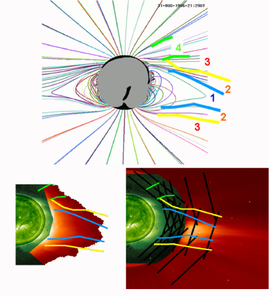
Figure 1: Top: Magnetic field lines map calculated by the 3D-MHD model with labeled regions and streamer boundaries defined in the text. The field lines shown are only those close to the plane of sky ($\pm$ 10 degrees). The coronal hole boundary (black regions) calculated from the photospheric magnetic maps is shown on the disk surface. Bottom: Composite images of the Sun: the disk is imaged with EIT in the FeXII 195 Å  line (green, disk); the limb images are obtained with the LASCO C1 coronagraph (green, off-limb) and the coronal images are obtained with UVCS OVI 1032 line (interpolated red image) with superposed the streamer boundaries (left panel) and LASCO C2 visible light (red outer image) with superposed the slit of UVCS (black lines) and the streamer boundaries (right panel).

In the case of the observation on August 31, the field of view of UVCS was well centered relative to the magnetic core of the streamer, derived from the MHD extrapolations. This is then selected for the analysis of the internal part of the streamer. The other dates of the UVCS observations, August 30 and September 1, 1996, are considered for the analysis of the open field regions just outside streamers. The observations on August 26 are used for the analysis of the regions at the edge of coronal hole.
The streamer boundary is defined as coincident with the interface between closed and open field lines obtained from the extrapolations of the photospheric magnetic field for the dates of observation of the streamers. The magnetic streamer boundaries are shown in Figure 1 as blue lines. The precision of the determination of the boundary depends on the resolution used in the magnetic model to extrapolate coronal field lines and in this way it depends on the accuracy of the model itself. The boundaries are then compared with those defined on the basis of the intensity of UV lines in the outer corona (Abbo and Antonucci 2002 and Antonucci et al. 2005). The streamer boundaries defined as the 1/e 1032 O VI peak intensity level, shown in Figure 1 as yellow lines, result to be external to those defined on the basis of the magnetic field model extrapolated from the photospheric data by $\sim$5-10^o. The 1/e intensity boundary has been considered in several previous work (e.g. Abbo et al. 2002, 2003a; Marocchi et al. 2001; Uzzo et al. 2003; Antonucci et al. 2005). This is a reasonable definition of the streamer boundary in absence of a direct inference of the magnetic topology of the coronal regions, as discussed in more details by Antonucci et al. 2005. The bottom panels of Figure 1 show both the solar disk imaged with EIT (Fe XII 195 Å) and the limb with LASCO C1 but, on the left, the coronal image is obtained with UVCS and, on the right, by LASCO C2. In order to derive the plasma conditions within the streamer, and in the external regions, the intensities of the O VI 1032 and 1038 lines are integrated in four regions shown in Figure 1 on the top panel: within the streamer magnetic boundaries (region 1), in the intermediate region between the magnetic and the OVI intensity boundaries (region 2, as defined before), in the region external to the OVI intensity boundary (region 3, defined between $\sim$288^o and $\sim$305^o) and in coronal hole (region 4, defined between $\sim$305^o and $\sim$320^o).
Stray light correction is applied and counts are transformed to intensity, $I(\lambda)$, by applying the standard radiometric calibration (Gardner et al. 1996). The integrated emissions are then fitted with a gaussian function, representing the coronal profile, convolved with a Lorentzian curve which accounts for the instrumental broadening and a rectangular function accounting for the width of the spectrometer slit. The function resulting from the convolution is added to a background linearly dependent on wavelength. The best fit is obtained by applying the least square method with the following quantities as adjustable parameters: standard deviation, $\sigma$, and mean wavelength, $\lambda_{0}$, of the solar profile, and slope and intercept of the background. Finally, the observed line intensity is derived as the integral over the gaussian line profile.
The electron density and the outflow velocity are derived from the ratio of the collisional to radiative component of the oxygen O VI 1032 line, with the constraint of mass flux conservation, according to the method discussed in section 2. The cross-section geometry of the flux tubes connecting the corona with the heliosphere, described by the expansion factor, is derived from the extrapolations of the coronal magnetic fields of the MHD model. Figure 2 shows the expansion factors relative to the flux tubes of the streamer boundaries derived for the observations (dashed and dash-dotted lines show the North-West and the South-West 1/e boundary, respectively, and dash-dot-dotted and dotted lines show the North-West and the South-West mhd boundary, respectively), compared with the expansion factors derived from the model of Wang & Sheeley (1990)(solid line), assumed in the analysis of Antonucci et al. (2005). We note that the increase around 2.5 R_⊙ is less marked in the expansion factors derived by Mikić et al. (1999). It has been suggested that there is a strong empirical anticorrelation between wind speed and expansion factors of magnetic flux tubes near the Sun (e.g. Levine et al. 1977; Wang and Sheeley 1990). Cranmer (2005) proposed a possible explanation of this effect by studying the critical points of the momentum function along flux tubes that range from the pole to the edge of the streamer belt. For what concerns the present work, the analyis of the latitudinal variation of the expansion factors will be investigated in details in a future work.

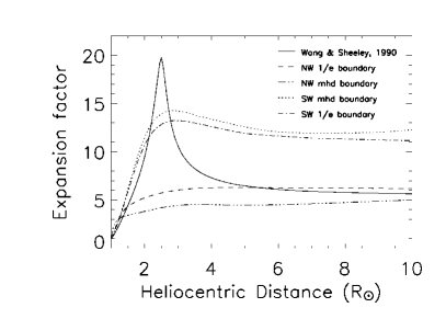
Figure 2: Expansion factors relative to the flux tubes of the streamer boundaries as a function of heliocentric distance: the solid curve refers to the model of Wang & Sheeley (1990), the other curves refer to model of Mikić et al. (1999) (dashed and dash-dotted lines show the North-West and the South-West 1/e boundary, respectively, and dash-dot-dotted and dotted lines show the North-West and the South-West mhd boundary, respectively), assumed in the present analysis.

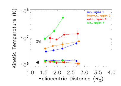
Figure 3: Kinetic temperature of O⁵⁺ ions and H⁰ atoms as a function of heliocentric distance for streamer (region 1, blue points) for region intermediate between the two boundaries (region 2, orange points), for the external region (region 3, red points) and for the base of coronal hole (region 4, green points).

The spectroscopic diagnostic technique can be applied when the distribution of the oxygen ion velocity in three dimensions is determined, since, in a given volume, the absorption of the photons of the exciting spectrum is controlled by the coronal absorption profile along the incident direction in a solid angle subtending the disk of the Sun. The solar wind is assumed to be radial and the velocity distribution along the two directions perpendicular to the radial is considered to be the same. The kinetic temperature of oxygen ions, $T_{k}$, expressed in terms of the spectral line width observed by UVCS, is a measure of the velocity distribution width along the l.o.s., while for the perpendicular directions to the l.o.s. has to be assumed (only for the fast wind in the core of coronal holes this quantity is partially constrained). Moreover, the derived kinetic temperature do not include the correction for removing the l.o.s. component of the outflow velocity. Figure 3 shows the kinetic temperature of O⁵⁺ ions and H⁰ atoms as a function of heliocentric distance for the four different regions as defined in Fig.1 (blue points for region 1, orange for region 2, red for region 3 and green for region 4). The data at 3.33 R_⊙ are not included because, in this case, it is difficult to determine the true widths of the line profiles using 300 $\mu$m for the UVCS slit width. It is reasonable to assume an isotropic maxwellian velocity distribution inside the streamer, with the width defined by the observed $T_{k}$. Within the streamer, the electron and ion densities are higher and due to the approximately static conditions of the plasma, the isotropy of the ion velocity distribution is established via ion-ion collision. Outside the streamer, in the regions 2, 3 and 4, where there is an open field line topology, a bi-maxwellian velocity distribution of the ions is assumed, as for the analysis of coronal holes. In this case, the ion kinetic temperature corresponds to the observed line width in the plane perpendicular to the radial direction, and the ion kinetic temperature along the radial direction is equal to the electron temperature (maximum anisotropy). This assumption is dictated by the fact that line broadening in the external regions (region 3) is about twice as larger than inside the streamer itself, thus representing an intermediate condition between closed field regions and the core region of coronal holes, where the ion velocity distributions are found to be highly anisotropic (e.g. Kohl et al., 1998, Cranmer et al., 1999b, Antonucci et al., 2000a and b). Also in the regions between the boundaries (region 2) we assume an anisotropic velocity distribution.
The coronal electron temperature, $T_{e}$, assumed in the analysis of streamers, is that derived by Gibson, et al. (1999) for the minimum of solar activity and varies between 1.5$\times 10^{6}$ K and 7$\times 10^{5}$ K in the range of distance 1.5–3.5 R_⊙. We note that the $T_{e}$ values do not influence significantly the results of the analysis of electron density and outflow velocity (see also Antonucci et al., 2000b). Therefore, in the absence of a direct measurement of $T_{e}$, we assume in the open field line regions the same electron temperature of coronal holes, as inferred from the coronal hole measurements by David et al. (1998) and extrapolated to the values by Ko et al. (1997) further out in the corona obtained from $in-situ$ charge-state measurements performed with the SWICS experiment. That is, we assume that the regions outside streamers are cooler than the internal regions, with temperatures which never exceed 1$\times 10^{6}$ K.

6 Results

We derive the electron density for the three regions inside and outside the streamer and for the region at the edge of the coronal hole as defined in Figure 1. The results are shown in Figure 4 and Table 2.

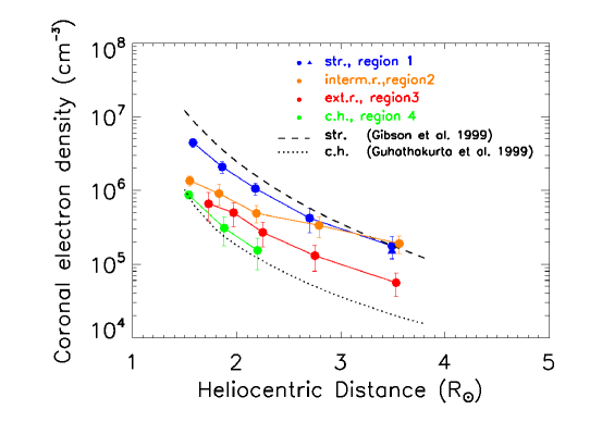
Figure 4: Electron density (cm^-3) as a function of heliocentric distance (in solar radii), calculated considering the region within the streamer boundaries (blue dots, region 1), the region between the boundaries (orange dots, region 2), the region external to the boundary defined as 1/e OVI intensity (red dots, region 3) and at the edge of coronal hole (green dots, region 4). The dashed line shows the values derived by Gibson et al. (1999) from visible light observations for streamers and the dotted line shows results obtained by Guhathakurta et al. (1999) for coronal holes. Static conditions are assumed in the streamer due to the presence of closed magnetic field; at 3.5 R_⊙, the blue triangle shows the result by assuming an expanding coronal plasma. The error bars have been estimated based on the propagation of the statistical uncertainties of the observed OVI 1032 and 1037 line intensities.

The electron density values relative to the inner part of the streamers (region 1, blue dots) are calculated assuming a static plasma. The values are compatible with those derived in streamers from the visible light coronal observations by Gibson et al. (1999) (dashed line). At 3.5 R_⊙, we obtain also a value (blue triangle) by assuming an expanding coronal plasma and an anisoptropic velocity distribution. For what concerns the regions external to the streamer boundaries (region 3), we have computed the electron density taking into account the magnetic topology of the flux tubes as derived by the MHD model and the results are shown as red dots in Fig. 4, compared with those derived for streamers by Gibson et al. (1999) (dashed line) and for coronal holes by Guhathakurta et al. (1999) (dotted line). The electron density values relative to the region between boundaries (region 2) and at the base of the coronal hole (region 4) are shown, respectively, as orange and green dots. The error bars do not include uncertainties in the MHD model, but are based on the propagation of the statistical uncertainties of the observed OVI 1032 and 1037 line intensities. The density and outflow velocity results however also depend on other factors, as discussed in Antonucci et al. 2004. The values in the regions 1 and 2 are comparable beyond 2.5 R_⊙. This fact (see also the T_k,OVI results in the previous section) suggests that the plasma of these regions could be the same, when the streamer converges to form the current sheet. The density results outside the streamer have intermediate values between those of a coronal hole and of the streamer and they are compatible with those obtained in the analysis of Antonucci et al. (2005). The region 4 is characterized by T_k,OVI and n_e values of the coronal hole core. Moreover, at 1.5 R_⊙ the electron density values in regions 2 and 3 are more similar to the coronal hole values than those in the streamer. These results are interesting for the analysis of the latitudinal variation of the physical parameters from slow to fast wind.
Figure 5 and Table 3 show the values of the outflow velocities as a function of heliocentric distance for regions 2, 3 and 4 and the velocity at one height (3.5 R_⊙) for streamer region 1. In Figure 5, they are extended to higher altitudes by including the white-light observations by LASCO (Sheeley et al., 1997) in the range from 4 to 10 R_⊙ (gray band). The values are much lower than those of the fast wind, which reaches 200 km/s at 2 R_⊙ and 400 km/s at 3 R_⊙. The solid curve represents the values obtained from the UVCS analysis in the center of coronal holes up to 3 R_⊙ and the dashed curves show the results by Telloni et al. (2007) on the fast wind velocity with two different hypotheses for the degree of anisotropy in the velocity distribution. The outflow velocity values vary between 90 and 120 km/s approximately and there is no significant difference between the outflow velocity values in region 2 and in region 3, but there is a considerable change of O VI kinetic temperature and electron density values from one region to the other one. For what concerns region 1, within the streamer, we found at 3.5 R_⊙  an outflow velocity value equal to 106$\pm$5 km/s. On the basis of the coronal field lines, at this height the current sheet is already formed. Hence, we find slow wind flowing along the axis of the streamer above the cusp. Finally, region 4 shows typical outflow velocity values of the coronal hole core. This fact indicates that, at the edge of coronal holes, the plasma has already reached the characteristics of the fast wind regime.

Table 2: Electron density averaged along the line-of-sight, $<n_{e}>$, derived for the three regions as a function of the height: the inner part of the streamer (region 1), the intermediate region between the two boundaries (region 2) and the region external to the 1/e intensity boundary (region 3).

Region 1 Region 2 r (R⊙) $<n_{e}>$ (cm-3) r (R⊙) $<n_{e}>$ (cm-3) 1.58 4.5$\pm$0.6 $\times$106 1.55 1.3$\pm$0.2 $\times$106 1.86 2.1$\pm$0.4 $\times$106 1.83 9.1$\pm$2.9 $\times$105 2.18 1.1$\pm$0.2 $\times$106 2.19 4.9$\pm$1.3 $\times$105 2.70 4.2$\pm$1.5 $\times$105 2.79 3.3$\pm$1.0 $\times$105 3.49 1.8$\pm$0.6 $\times$105 3.56 1.90$\pm$0.5 $\times$105 3.491 1.5$\pm$0.3 $\times$105 Region 3 Region 4 r (R⊙) $<n_{e}>$ (cm-3) r (R⊙) $<n_{e}>$ (cm-3) 1.73 6.6$\pm$2.8 $\times$105 1.54 8.7$\pm$1.1 $\times$105 1.97 5.0$\pm$1.8 $\times$105 1.88 3.1$\pm$1.3 $\times$105 2.25 2.7$\pm$1.1 $\times$105 2.2 1.5$\pm$0.7 $\times$105 2.75 1.3$\pm$0.5 $\times$105 3.53 5.6$\pm$2.0 $\times$104

¹ with the assumption of an expanding coronal plasma.

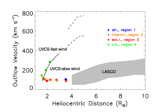
Figure 5: Outflow velocity (km/s) of the slow wind for the considered four regions as a function of the heliocentric distance (in solar radii). The grey band from 4 to 10 R_⊙ shows the range of outflow velocities for the slow wind obtained with LASCO (Sheeley et al., 1997). The solid curve up to 3 R_⊙ represents the values of the fast wind obtained from the UVCS data (Antonucci et al., 2000b) and the dashed curves show the results by Telloni et al. (2007) of the fast wind velocity. The error bars (small in many cases) have been estimated based on the propagation of the statistical uncertainties of the observed OVI 1032 and 1037 line intensities.

Table 3: Outflow velocity (km/s) of the slow wind as a function of heliocentric distance (in solar radii) for the intermediate and the external regions (see text for details).

Region 2		Region 3		Region 4
r (R⊙)	vout (km/s)	r (R⊙)	vout (km/s)	r (R⊙)	vout (km/s)
1.65	117.5$\pm$10	1.73	110$\pm$5	1.54	145$\pm$20
1.83	103$\pm$10	1.97	90$\pm$10	1.88	199$\pm$30
2.19	100$\pm$5	2.25	101$\pm$5	2.2	283$\pm$30
2.79	93$\pm$5	2.75	100$\pm$5
3.56	100$\pm$5	3.53	90$\pm$10

7 Conclusions

The results of kinetic temperature, electron density and ion outflow velocity in the streamer belt of the minimum corona (1996) lead to a more accurate identification of the sources of the slow coronal wind than in previous analyses. The slow wind is found, mainly, to flow adjacent to the streamer boundary in the open magnetic field line region. Moreover, the presence of outflowing plasma has been detected where the heliospheric current sheet is forming, approximately beyond 3.5 R_⊙. These results while confirming, to a large degree, those of Antonucci et al. (2005), show that the region where the slow wind is observed is more extended toward the streamer, since the mhd boundary is closer to the streamer axis than the 1/e instensity boundary. In the previous paper, the authors suggested that the open field lines running along the streamer boundary originate in the same unipolar magnetic region lying at the base of a polar coronal hole, because the regions just outside the streamer boundary are characterized by the same density as the hole edge below 2 R_⊙. The present analysis confirms this hypothesis: the density values of regions 2,3 and 4 are comparable around 1.5 R_⊙, while further out in the corona, the density varies significantly from the coronal hole edge toward the streamer.
The outflow velocity values are comparable with those derived by Sheeley et al. (1997), from the white-light observations of LASCO between 2 R_⊙ and 5 R_⊙. The values of electron density and outflow velocity in the streamer adjacent regions are consistent with those found by Antonucci et al. (2005) up to 2.75 R_⊙. At 3.5 R_⊙ the values of $<n_{e}>$ are lower in the present analysis with consequently higher outflow velocity values. We note that in this range of heights (2.5–3.5 R_⊙), the coronal expansion factors assumed in the two studies have a different behaviour (see Fig. 2). The outflow velocity results of the present analysis are consistent with those found by Strachan et al. (2002): they analysed the visible and ultraviolet coronal emission of an equatorial streamer, using the Doppler dimming technique, along the streamer axis from 2.3 R_⊙ to 5.1 R_⊙, and across the streamer, but only at 2.33 R_⊙. They obtained outflows as a function of height along the streamer axis with values ranging from about 50 to 100 km/s from 4.1 to 5.1 solar radii. There were no detectable outflows along the streamer axis below 3.5 R_⊙. Outflow velocities from 50-110 km/s were detected only outside $\sim$15 degrees from the streamer axis at 2.33 R_⊙. In our analysis of the regions along the streamer axis, the outflow velocities are higher, in the range within (100-110 km/s), and are observed at lower heights, at 3.5 R_⊙. The difference between the results of the two studies can be traced to the fact that the values of the inferred electron densities are different. In this study n_e and w are derived using the same observations. The density used by Strachan et al. (2002) is inferred from visible light data which usually yields higher values.
The results of our analysis suggest that the slow wind flows externally to the bright parts of the streamer called ’legs’, proposed as coronal sources of the slow wind by i.e. Raymond et al. (1997) and Uzzo et al. (2003) and there is no detectable wind contribution coming from these structures, thus it can be deduced that they are characterized by a closed magnetic topology. The scenario resulting from the identification of the slow wind sources with the regions surrounding the streamer boundaries and possibly with the region close to the current sheet, is compatible with the model proposed by Wang et al. (2000), of a two–component slow wind: one component flowing along the rapidly diverging open magnetic field lines adjacent to the streamer boundary, and the second one confined to the region of the denser equatorial plasma sheet. The latter case has the same observational characteristics as the model of Noci et al. (1997).

8 Acknowledgments

UVCS is a joint project of the National Aeronautics and Space Administration (NASA), the Agenzia Spaziale Italiana (ASI) and Swiss Founding Agencies. The research of LA has been funded through the contract I/023/09/0 between the National Institute for Astrophysics (INAF) and the Italian Space Agency (ASI) and also through the contract ASI/I/035/05/0, by Agenzia Spaziale Italiana and Ministero dell’Istruzione, dell’Università e della Ricerca. The work at Predictive Science, Inc. was partially supported by NASA’s Heliophysics Theory and SR & T programs, and NSF’s CISM program.

References

- Abbo (2002) Abbo, L., & Antonucci, E. 2002, in Second Solar Cycle and Space Weather Euroconference, ed. H. Sawaya-Lacoste (ESA SP-477; Noordwijk: ESA), 323
- Abbo (2002) Abbo, L. 2002, Ph.D. Thesis, University of Torino
- Abbo et al. (2003a) Abbo, L., Antonucci, E., Dodero, M.A. & Benna, C. 2003a, in Solar Wind 10, AIP Conf. Proc., 679, 238
- Abbo et al. (2003b) Abbo, L., Antonucci, E., Mikic̀ , Z., Riley, P, Dodero, M.A. & Giordano, S.2003b, Memorie della Società Astronomica Italiana, 74, 733
- Antonucci et al. (1997) Antonucci, E., Noci, G., Kohl, J.L., et al. 1997, ASP Conference Series, 118, 273
- Antonucci et al. (2000a) Antonucci, E., Giordano, S., & Dodero, M. A. 2000a, Advances in Space Research, 25, 1923
- Antonucci et al. (2000b) Antonucci, E., Dodero, M.A. & Giordano, S. 2000b, Sol. Phys., 197, 115
- Antonucci et al. (2004) Antonucci, E., Dodero, M.A., Giordano, S., et al. 2004, A&A, 416, 749
- Antonucci et al. (2005) Antonucci, E., Abbo, L. & Dodero, M.A. 2005, A&A, 435, 699
- Antonucci et al. (2006) Antonucci, E., Abbo, L. & Telloni, D. 2006, ApJ, 643, 1239
- Beckers (1974) Beckers, J.M. & Chipman, E. 1974, Sol. Phys., 34, 151
- Curdt (2001) Curdt, W., Brekke, P., Feldman, U. ,et al. 2001, A&A, 375, 591
- Cranmer (1999a) Cranmer, S.R., Kohl, J.L., Noci, G., et al. 1999a, ApJ, 511, 481
- Cranmer (1999b) Cranmer, S.R., Field, G.B. & Kohl, J.L. 1999b, ApJ, 518, 937
- Cranmer (2005) Cranmer, S.R. 2005, Proceedings of the Solar Wind 11 / SOHO 16, ”Connecting Sun and Heliosphere” Conference (ESA SP-592), 159
- David et al. (1998) David, C., Gabriel, A. H., Bely-Dubau, F., et al. 1998, A&A, 336, L90
- Dobrzycha et al. (1999) Dobrzycka, D., Cranmer, S.R, Panasyuk, A.V., et al., 1999, JGR, 104, 9791
- Dodero et al. (1998) Dodero, M.A., Antonucci, E., Giordano, S., et al. 1998, Sol. Phys, 183, 77
- Fisk et al. (1999) Fisk, L.A., Zurbuchen, T.H. & Schwadron, N.A. 1999, ApJ, 521, 868
- Frazin, Cranmer, & Kohl (2003) Frazin, R. A., Cranmer, S. R., & Kohl, J. L. 2003, ApJ, 597, 1145
- Gardner et al. (1996) Gardner, L.D., Kohl, J.L, Daigneau, P.S., et al. 1996, Proc. SPIE, 2831, 2
- Gibson et al. (1999) Gibson, S. E., Fludra, A., Bagenal, F., et al. 1999, JGR, 104, 9691
- Guhathakurta et al. (1999) Guhathakurta, M., Fludra, A., Gibson, S.E., et al. 1999, JGR, 104, 9801
- Habbal et al. (1997) Habbal, S.R., Woo, R., Fineschi, S., et al. 1997, ApJ, 489, L103
- Kohl et al. (1982) Kohl, J.L. & Withbroe, G.L. 1982, ApJ, 256, 263
- Kohl et al. (1995) Kohl, J. L., Esser, R., Gardner, L. D., et al. 1995, Sol. Phys., 162, 313.
- Kohl et al. (1998) Kohl, J.L., Noci, G., Antonucci, E., et al. 1998, ApJ, 501, L127
- Lionello et al. (2009) Lionello, R., Linker, J.A., Mikic̀ , Z. 2009, ApJ, 690, 902
- Li et al. (1998) Li, X., Habbal, S.R., Kohl, J., et al. 1998, ApJ, 501, L133
- Linker et al. (1999) Linker, J.A., Mikic̀ , Z., Biesecker, D.A., et al. 1999, JGR, 104, 9809
- Marocchi et al. (2001) Marocchi, D., Antonucci, E. & Giordano, S. 2001, Ann.Geophys., 19, 135
- Mikic et al. (1999) Mikic̀ , Z., Linker, J.A., Schnack, D.D, et al. 1999, Phys.of Plasmas, 6, 5
- Noci et al. (1987) Noci, G., Kohl, J.L. & Withbroe, G.L. 1987, ApJ, 315, 706
- Noci et al. (1997) Noci, G., Kohl, J.L., Antonucci, E., et al. 1997, in Fifth SOHO Workshop, The Corona and Solar Wind near Minimum Activity, ed. A. Wilson (ESA SP-404; Noordwijk: ESA), 75
- Noci (2007) Noci, G. & Gavryuseva, E. 2007, ApJ, 658, L63
- Ofman (2000) Ofman, L. 2000, Geophys. Res. Let., 27, 18, 2885
- Parenti (2000) Parenti, S., Bromage, B.J.I., Poletto, G., et al. 2000, A&A, 363, 800
- Poletto (2002) Poletto, G., Suess,S. T., Biesecker, et al. 2002, JGR, 107, 9
- Raymond et al. (1997) Raymond, J.C., Kohl, J.L., Noci, G., et al. 1997, Sol. Phys., 175, 645
- Sheeley et al. (1997) Sheeley, N.R., Jr., Wang, Y.-M., Hawley, S.H., et al. 1997, ApJ, 484, 472
- Spadaro et al. (2005) Spadaro, D., Ventura, R., Cimino, G., & Romoli, M. 2005, A&A, 429, 353
- Strachan et al. (2000) Strachan, L., Panasyuk, A.V., Dobrzycka, D., et al. 2000, JGR, 105, 2345
- Strachan et al. (2002) Strachan, L., Suleiman, R., Panasyuk, A.V., et al. 2002, ApJ, 571, 1008
- Telloni et al. (2007) Telloni, D., Antonucci, E., & Dodero, M.A. 2007, A&A, 472, 299
- Uzzo et al. (2003) Uzzo, M., Ko, Y.-K., Raymond, J.C., et al. 2003, ApJ, 585, 1062
- Wang et al. (1990) Wang, Y.H. & Sheeley, N.R., Jr. 1990, ApJ, 355, 726
- Wang et al. (1998) Wang, Y.-M., Sheeley, N. R., Jr., Walters, J. H., et al. 1998, ApJ, 498, L165
- Wang et al. (2000) Wang, Y.-M., Sheeley, N.R., Jr., Socker, D.G., et al. 2000, JGR, 105, 25133
- Wiegelmann et al. (2000) Wiegelmann, T., Schindler, K. & Neukirch, T. 2000, Sol. Phys., 191(2), 391
- Withbroe et al. (1982) Withbroe, G.L., Kohl, J.L.,, Weiser, H., et al. 1982, Space Science Rev, 33, 17
- Zangrilli et al. (1999) Zangrilli, L., Nicolosi, P., Poletto, G., et al. 1999, A&A, 342, 592