Analysis of the scalar and axial-vector heavy diquark states with QCD sum rules

Zhi-Gang Wang 111E-mail:wangzgyiti@yahoo.com.cn.

Department of Physics, North China Electric Power University, Baoding 071003, P. R. China

Abstract

In this article, we study the mass spectrum of the scalar and axial-vector heavy diquark states with the QCD sum rules in a systematic way. Once the reasonable values are obtained, we can take them as basic parameters and study the new charmonium-like states as the tetraquark states.

PACS numbers: 12.38.Lg; 13.25.Jx; 14.40.Cs

Key Words: Diquark states, QCD sum rules

1 Introduction

The scattering amplitude for one-gluon exchange in an $SU(N_{c})$ gauge theory is proportional to

$\displaystyle T^{a}_{ki}T^{a}_{lj}$ $\displaystyle=$ $\displaystyle-\frac{N_{c}+1}{4N_{c}}(\delta_{jk}\delta_{il}-\delta_{ik}\delta_{jl})+\frac{N_{c}-1}{4N_{c}}(\delta_{jk}\delta_{il}+\delta_{ik}\delta_{jl})\,,$ (1)

where the $T^{a}$ is the generator of the gauge group, and the $i,j$ and $k,l$ are the color indexes of the two quarks in the incoming and outgoing channels respectively. For $N_{c}=3$, the negative sign in front of the antisymmetric antitriplet indicates the interaction is attractive, while the positive sign in front of the symmetric sextet indicates the interaction is repulsive [1]. The attractive interaction favors the formation of the diquark states in the color antitriplet, and the most stable diquark states maybe exist in the color antitriplet $\overline{\bf{3}}_{c}$, flavor antitriplet $\overline{\bf{3}}_{f}$ and spin singlet ${\bf{1}}_{s}$ channels due to Fermi-Dirac statistics [2]. On the other hand, the study based on the random instanton liquid model indicates that the instanton induced quark-quark interactions are weakly repulsive in the vector and axial-vector channels, strongly repulsive in the pseudoscalar channel, and strongly attractive in the scalar and tensor channels [3].

The conception of diquarks has many phenomenological applications [4, 5, 6], for example, the quark-diquark bound states scenario of the ground state baryons [7], the $\Delta I=\frac{1}{2}$ rule in the non-leptonic weak decays [8], the $4:1$ ratio of the proton and neutron deep inelastic structure functions in the limit $x\to 1$ [9], the color superconductivity in the cold dense quark matters [10].

Taking the diquarks as basic constituents, we can obtain a new spectroscopy for the mesons and baryons [11, 12]. The numerous candidates with $J^{PC}=0^{++}$ below $2\,\rm{GeV}$ cannot be accommodated in one $q\bar{q}$ nonet, some are supposed to be glueballs, molecular states and tetraquark states [5, 13, 14]. The $a(980)$ and $f(980)$ are good candidates for the $K{\bar{K}}$ molecular states [15], however, their cousins $\sigma(600)$ and $\kappa(800)$ lie considerably higher than the corresponding thresholds, it is difficult to identify them as the $\pi\pi$ and $\pi K$ molecular states respectively. There maybe different dynamics dominating the $0^{++}$ mesons below and above $1\,\rm{GeV}$ which result in two scalar nonets below $1.7\,\rm{GeV}$. The strong attractions between the diquark states $(qq)_{\overline{3}}$ and $(\bar{q}\bar{q})_{3}$ in $S$-wave may result in a nonet tetraquark states manifested below $1\,\rm{GeV}$. The conventional ${}^{3}P_{0}$ $\bar{q}q$ nonet would have masses about $(1.2-1.6)\,\rm{GeV}$, and the well established ${}^{3}P_{1}$ and ${}^{3}P_{2}$ $\bar{q}q$ nonets with $J^{PC}=1^{++}$ and $2^{++}$ respectively lie in the same region. Furthermore, there are enough candidates for the ${}^{3}P_{0}$ $\bar{q}q$ nonet mesons, $a_{0}(1450)$, $f_{0}(1370)$, $K^{*}(1430)$, $f_{0}(1500)$ and $f_{0}(1710)$ [5, 13, 14].

In the tetraquark models, the structures of the nonet scalar mesons in the ideal mixing limit can be symbolically written as

$\displaystyle\sigma(600)=ud\bar{u}\bar{d},\;$ $\displaystyle f_{0}(980)={us\bar{u}\bar{s}+ds\bar{d}\bar{s}\over\sqrt{2}},$
$\displaystyle a_{0}^{-}(980)=ds\bar{u}\bar{s},\;$ $\displaystyle a_{0}^{0}(980)={us\bar{u}\bar{s}-ds\bar{d}\bar{s}\over\sqrt{2}},\;a_{0}^{+}(980)=us\bar{d}\bar{s},$
$\displaystyle\kappa^{+}(800)=ud\bar{d}\bar{s},\;$ $\displaystyle\kappa^{0}(800)=ud\bar{u}\bar{s},\;\;\;\;\;\;\bar{\kappa}^{0}(800)=us\bar{u}\bar{d},\;\;\;\;\;\;\kappa^{-}(800)=ds\bar{u}\bar{d}.$

The four light isospin-$\frac{1}{2}$ $K\pi$ resonances near $800\,\rm{MeV}$, known as the $\kappa(800)$ mesons, have not been firmly established yet, there are still controversy about their existence due to the large width and nearby $K\pi$ threshold [16]. The E791 collaboration observed a low-mass scalar $K\pi$ resonance with the Breit-Wigner mass $(797\pm 19\pm 43)\,\rm{MeV}$ and width $(410\pm 43\pm 87)\,\rm{MeV}$ in the decay $D^{+}\to K^{-}\pi^{+}\pi^{+}$ [17], and the BES collaboration observed a clear low mass enhancement in the invariant $K\pi$ mass distribution in the decay $J/\psi\to\bar{K}^{*}(892)K^{+}\pi^{-}$ with the Breit-Wigner mass $(878\pm 23^{+64}_{-55})\,\rm{MeV}$ and width $(499\pm 52^{+55}_{-87})\,\rm{MeV}$ [18]. Recently, the BES collaboration reported the charged $\kappa(800)$ in the decay $J/\psi\to K^{*}(892)^{\mp}K_{s}\pi^{\pm}$ with the Breit-Wigner mass $(826\pm 49_{-34}^{+49})\,\rm{MeV}$ and width $(449\pm 156_{-81}^{+144})\,\rm{MeV}$ [19].

In general, we may expect constructing the tetraquark currents and studying the nonet scalar mesons below $1\,\rm{GeV}$ as the tetraquark states with the QCD sum rules approach [20, 21], which is powerful tool in studying the ground state hadrons. For the conventional mesons and baryons, the ”single-pole + continuum states” model works well in representing the phenomenological spectral densities, the continuum states are usually approximated by the contributions from the asymptotic quarks and gluons, the Borel windows are rather large and reliable QCD sum rules can be obtained. However, for the light flavor tetraquark states (and pentaquark states, for example, the $\Theta(1540)$), we cannot obtain a Borel window to satisfy the two criteria (pole dominance and convergence of the operator product expansion) of the QCD sum rules [22]. For the heavy tetraquark states and molecular states, the two criteria can be satisfied, but the Borel windows are rather small [23, 24].

We can take the colored diquarks as point particles and describe them as the scalar, pseudoscalar, vector, axial-vector and tensor fields respectively to overcome the embarrassment [25]. In Ref.[26], we construct the color singlet tetraquark currents with the scalar diquark fields, take the diquark masses as the basic parameters, parameterize the nonperturbative effects with the new vacuum condensates besides the gluon condensate, and perform the standard procedure of the QCD sum rules to study the nonet scalar mesons below $1\,\rm{GeV}$, the numerical results are satisfactory.

In recent years, the Babar, Belle, CLEO, D0, CDF and FOCUS collaborations have discovered (or confirmed) a large number of charmonium-like states, and revitalized the interest in the spectroscopy of the charmonium states [27]. For example, Maiani et al identify the $X(3872)$ observed by the Belle collaboration [28] as a $1^{++}$ state with the diquark-antidiquark structure $[cq]_{S=1}[{\bar{c}}{\bar{q}}]_{S=0}+[cq]_{S=0}[{\bar{c}}{\bar{q}}]_{S=1}$ [29]. The $Z(4430)$ and $Z(4050)$, $Z(4250)$ observed in the decay modes $\psi^{\prime}\pi^{+}$ and $\chi_{c1}\pi^{+}$ respectively by the Belle collaboration are the most interesting subjects [30, 31, 32]. They can’t be pure $c\bar{c}$ states due to the positive charge, and may be $c\bar{c}u\bar{d}$ tetraquark states (irrespective of the molecule type and the diquark-antidiquark type).

In Refs.[33, 34], the mass spectrum of the scalar light diquark states are studied using the QCD sum rules. So it is interesting to study the scalar and axial-vector heavy diquark states with the QCD sum rules. Once reasonable values of the heavy diquark masses are obtained, we can take them as basic parameters and study the new charmonium-like states as the tetraquark states.

There have been several theoretical approaches to deal with the heavy diquark masses, such as the relativistic quark model based on a quasipotential approach in QCD [35], the Bethe-Salpeter equation [36], the constituent diquark model [29, 37, 38], etc.

The article is arranged as follows: we derive the QCD sum rules for the scalar and axial-vector heavy diquark states in Sect.2; in Sect.3, we present the numerical results and discussions; and Sect.4 is reserved for our conclusions.

2 The scalar and axial-vector heavy diquark states with QCD Sum Rules

In the following, we write down the interpolating currents for the scalar and axial-vector heavy diquark states,

$\displaystyle J^{i}(x)$ $\displaystyle=$ $\displaystyle\epsilon^{ijk}q_{j}^{T}(x)C\gamma_{5}Q_{k}(x)\,,$
$\displaystyle\eta^{i}(x)$ $\displaystyle=$ $\displaystyle\epsilon^{ijk}s_{j}^{T}(x)C\gamma_{5}Q_{k}(x)\,,$
$\displaystyle J^{i}_{\mu}(x)$ $\displaystyle=$ $\displaystyle\epsilon^{ijk}q_{j}^{T}(x)C\gamma_{\mu}Q_{k}(x)\,,$
$\displaystyle\eta^{i}_{\mu}(x)$ $\displaystyle=$ $\displaystyle\epsilon^{ijk}s_{j}^{T}(x)C\gamma_{\mu}Q_{k}(x)\,,$ (2)

the $i,~{}j,~{}k$ are color indexes, $Q=b,~{}c$, and the $C$ is the charge conjugation matrix.

The two-point correlation functions $\Pi(p)$ and Πμ​ν​(p)subscriptΞ πœ‡πœˆπ‘\Pi_{\mu\nu}(p) can be written as

$\displaystyle\Pi(p)$ $\displaystyle=$ $\displaystyle i\int d^{4}x~{}e^{ip.x}\langle 0|T[J(x)J^{\dagger}(0)]|0\rangle\,,$
Πμ​ν​(p)subscriptΞ πœ‡πœˆπ‘\displaystyle\Pi_{\mu\nu}(p) $\displaystyle=$ iβ€‹βˆ«d4​x​ei​p.xβ€‹βŸ¨0|T​[Jμ​(x)​Jν†​(0)]|0⟩,𝑖superscript𝑑4π‘₯superscript𝑒formulae-sequence𝑖𝑝π‘₯quantum-operator-product0𝑇delimited-[]subscriptπ½πœ‡π‘₯superscriptsubscriptπ½πœˆβ€ 00\displaystyle i\int d^{4}x~{}e^{ip.x}\langle 0|T[J_{\mu}(x)J_{\nu}^{\dagger}(0)]|0\rangle\,, (3)

where the currents $J(x)$ and $J_{\mu}(x)$ denote the $J^{i}(x)$, $\eta^{i}(x)$ and $J^{i}_{\mu}(x)$, $\eta^{i}_{\mu}(x)$ respectively.

The one-gluon exchange results in strong attractions in the color antitriplet channel $\bar{\bf{3}}_{c}$, the quark-quark system maybe form quasibound states (diquark states) which are characterized by the correlation length $\mathbb{L}$. At the distance $l>\mathbb{L}$, the $\bar{\bf{3}}_{c}$ diquark state combines with the one quark or one $\bf{3}_{c}$ antidiquark to form a baryon state or a tetraquark state, while at the distance $l<\mathbb{L}$, the $\bar{\bf{3}}_{c}$ diquark states dissociate into asymptotic quarks and gluons gradually. We carry out the operator product expansion at not so deep Euclidean space where the approximation of the correlation functions by the perturbative contributions and the vacuum condensates makes sense. If we take the diquark state as an effective colored hadron and the diquark mass as an effective quantity, $M_{\mathbb{D}}\sim\frac{1}{\mathbb{L}}$, the correlation function can be continued to the physical region, where the quark-quark correlations exist, although the diquarks are not asymptotic states, there are significant differences between the diquark states and conventional hadrons. The correlation functions are approximated by a pole term plus a perturbative continuum.

We can insert a complete set of intermediate ”hadronic” states (effective hadron states) with the same quantum numbers as the current operators into the correlation functions to obtain the ”hadronic” representation [20]. Isolating the ground state contributions from the pole terms of the scalar and axial-vector heavy diquarks, we get the results,

$\displaystyle\Pi(p)$ $\displaystyle=$ βˆ«Ξ”2βˆžπ‘‘s​ρS​(s)sβˆ’p2,superscriptsubscriptsuperscriptΞ”2differential-d𝑠subscriptπœŒπ‘†π‘ π‘ superscript𝑝2\displaystyle\int_{\Delta^{2}}^{\infty}ds\frac{\rho_{S}(s)}{s-p^{2}}\,,
Πμ​ν​(p)subscriptΞ πœ‡πœˆπ‘\displaystyle\Pi_{\mu\nu}(p) $\displaystyle=$ βˆ«Ξ”2βˆžπ‘‘s​ρA​(s)sβˆ’p2​(βˆ’gμ​ν+pμ​pΞ½p2)+β‹―,superscriptsubscriptsuperscriptΞ”2differential-d𝑠subscriptπœŒπ΄π‘ π‘ superscript𝑝2subscriptπ‘”πœ‡πœˆsubscriptπ‘πœ‡subscriptπ‘πœˆsuperscript𝑝2β‹―\displaystyle\int_{\Delta^{2}}^{\infty}ds\frac{\rho_{A}(s)}{s-p^{2}}\left(-g_{\mu\nu}+\frac{p_{\mu}p_{\nu}}{p^{2}}\right)+\cdots\,, (4)
ρS​(s)subscriptπœŒπ‘†π‘ \displaystyle\rho_{S}(s) $\displaystyle=$ Ξ»S2​δ​(sβˆ’MS2)+Im​Π​(s)Ο€|perβ€‹Ξ˜β€‹(sβˆ’s0),superscriptsubscriptπœ†π‘†2𝛿𝑠superscriptsubscript𝑀𝑆2evaluated-atImΞ π‘ πœ‹perΞ˜π‘ subscript𝑠0\displaystyle\lambda_{S}^{2}\delta(s-M_{S}^{2})+\frac{{\rm{Im}}\Pi(s)}{\pi}|_{\rm{per}}\Theta(s-s_{0})\,,
ρA​(s)subscriptπœŒπ΄π‘ \displaystyle\rho_{A}(s) $\displaystyle=$ Ξ»A2​δ​(sβˆ’MA2)+Im​Πμ​ν​(s)Ο€|perβ€‹Ξ˜β€‹(sβˆ’s0),superscriptsubscriptπœ†π΄2𝛿𝑠superscriptsubscript𝑀𝐴2evaluated-atImsubscriptΞ πœ‡πœˆπ‘ πœ‹perΞ˜π‘ subscript𝑠0\displaystyle\lambda_{A}^{2}\delta(s-M_{A}^{2})+\frac{{\rm{Im}}\Pi_{\mu\nu}(s)}{\pi}|_{\rm{per}}\Theta(s-s_{0})\,, (5)

where the pole residues $\lambda_{S}$ and $\lambda_{A}$ (to be more precise, the current-diquark coupling strengths) are defined as

$\displaystyle\langle 0|{J/\eta}^{i}(0)|S^{j}(p)\rangle$ $\displaystyle=$ $\displaystyle\lambda_{S}\delta_{ij}\,,$
$\displaystyle\langle 0|{J/\eta}^{i}_{\mu}(0)|A^{j}(p)\rangle$ $\displaystyle=$ $\displaystyle\lambda_{A}\epsilon_{\mu}\delta_{ij}\,,$ (6)

the $\epsilon_{\mu}$ is the polarization vector, the $\Delta^{2}$ is the threshold parameter, the $s_{0}$ is the continuum threshold parameter, and the $\rm{per}$ denotes the perturbative contributions in the operator product expansion.

In the following, we briefly outline the operator product expansion for the correlation functions in perturbative QCD. The calculations are performed at large space-like momentum region $p^{2}\ll 0$, which corresponds to small distance $x\approx 0$ required by validity of operator product expansion. We write down the ”full” propagators $S_{ij}(x)$ and $S_{Q}^{ij}(x)$ of a massive quark in the presence of the vacuum condensates firstly [21],

$\displaystyle S_{ij}(x)$ $\displaystyle=$ i​δi​j​​x2​π2​x4βˆ’Ξ΄i​j​ms4​π2​x2βˆ’Ξ΄i​j12β€‹βŸ¨s¯​s⟩+i​δi​j48​msβ€‹βŸ¨s¯​sβŸ©β€‹β€‹xβˆ’Ξ΄i​j​x2192β€‹βŸ¨s¯​gs​σ​G​sβŸ©π‘–subscript𝛿𝑖𝑗π‘₯2superscriptπœ‹2superscriptπ‘₯4subscript𝛿𝑖𝑗subscriptπ‘šπ‘ 4superscriptπœ‹2superscriptπ‘₯2subscript𝛿𝑖𝑗12delimited-βŸ¨βŸ©Β―π‘ π‘ π‘–subscript𝛿𝑖𝑗48subscriptπ‘šπ‘ delimited-βŸ¨βŸ©Β―π‘ π‘ π‘₯subscript𝛿𝑖𝑗superscriptπ‘₯2192delimited-βŸ¨βŸ©Β―π‘ subscriptπ‘”π‘ πœŽπΊπ‘ \displaystyle\frac{i\delta_{ij}\!\not\!{x}}{2\pi^{2}x^{4}}-\frac{\delta_{ij}m_{s}}{4\pi^{2}x^{2}}-\frac{\delta_{ij}}{12}\langle\bar{s}s\rangle+\frac{i\delta_{ij}}{48}m_{s}\langle\bar{s}s\rangle\!\not\!{x}-\frac{\delta_{ij}x^{2}}{192}\langle\bar{s}g_{s}\sigma Gs\rangle
+i​δi​j​x21152​msβ€‹βŸ¨s¯​gs​σ​G​sβŸ©β€‹β€‹xβˆ’i32​π2​x2​gs​Gμ​νi​j​(​x​σμ​ν+σμ​ν​​x)+β‹―,𝑖subscript𝛿𝑖𝑗superscriptπ‘₯21152subscriptπ‘šπ‘ delimited-βŸ¨βŸ©Β―π‘ subscriptπ‘”π‘ πœŽπΊπ‘ π‘₯𝑖32superscriptπœ‹2superscriptπ‘₯2subscript𝑔𝑠subscriptsuperscriptπΊπ‘–π‘—πœ‡πœˆπ‘₯superscriptπœŽπœ‡πœˆsuperscriptπœŽπœ‡πœˆπ‘₯β‹―\displaystyle+\frac{i\delta_{ij}x^{2}}{1152}m_{s}\langle\bar{s}g_{s}\sigma Gs\rangle\!\not\!{x}-\frac{i}{32\pi^{2}x^{2}}g_{s}G^{ij}_{\mu\nu}(\!\not\!{x}\sigma^{\mu\nu}+\sigma^{\mu\nu}\!\not\!{x})+\cdots\,,
$\displaystyle S_{Q}^{ij}(x)$ $\displaystyle=$ $\displaystyle\frac{i}{(2\pi)^{4}}\int d^{4}ke^{-ik\cdot x}\left\{\frac{\delta_{ij}}{\!\not\!{k}-m_{Q}}-\frac{g_{s}G^{\alpha\beta}_{ij}}{4}\frac{\sigma_{\alpha\beta}(\!\not\!{k}+m_{Q})+(\!\not\!{k}+m_{Q})\sigma_{\alpha\beta}}{(k^{2}-m_{Q}^{2})^{2}}\right.$ (7)
$\displaystyle\left.+\frac{\pi^{2}}{3}\langle\frac{\alpha_{s}GG}{\pi}\rangle\delta_{ij}m_{Q}\frac{k^{2}+m_{Q}\!\not\!{k}}{(k^{2}-m_{Q}^{2})^{4}}+\cdots\right\}\,,$

where ⟨s¯​gs​σ​G​s⟩=⟨s¯​gs​σα​β​Gα​β​s⟩delimited-βŸ¨βŸ©Β―π‘ subscriptπ‘”π‘ πœŽπΊπ‘ delimited-βŸ¨βŸ©Β―π‘ subscript𝑔𝑠subscriptπœŽπ›Όπ›½superscript𝐺𝛼𝛽𝑠\langle\bar{s}g_{s}\sigma Gs\rangle=\langle\bar{s}g_{s}\sigma_{\alpha\beta}G^{\alpha\beta}s\rangle and ⟨αs​G​GΟ€βŸ©=⟨αs​Gα​β​GΞ±β€‹Ξ²Ο€βŸ©delimited-⟨⟩subscriptπ›Όπ‘ πΊπΊπœ‹delimited-⟨⟩subscript𝛼𝑠subscript𝐺𝛼𝛽superscriptπΊπ›Όπ›½πœ‹\langle\frac{\alpha_{s}GG}{\pi}\rangle=\langle\frac{\alpha_{s}G_{\alpha\beta}G^{\alpha\beta}}{\pi}\rangle, then contract the quark fields in the correlation functions with Wick theorem, and obtain the result:

$\displaystyle\Pi(p)$ $\displaystyle=$ $\displaystyle-i\epsilon^{ijk}\epsilon^{ij^{\prime}k^{\prime}}\int d^{4}x\,e^{ip\cdot x}Tr\left\{\gamma_{5}S_{Q}^{jj^{\prime}}(x)\gamma_{5}CS^{T}_{kk^{\prime}}(x)C\right\}\,,$
Πμ​ν​(p)subscriptΞ πœ‡πœˆπ‘\displaystyle\Pi_{\mu\nu}(p) $\displaystyle=$ $\displaystyle i\epsilon^{ijk}\epsilon^{ij^{\prime}k^{\prime}}\int d^{4}x\,e^{ip\cdot x}Tr\left\{\gamma_{\mu}S_{Q}^{jj^{\prime}}(x)\gamma_{\nu}CS^{T}_{kk^{\prime}}(x)C\right\}\,.$ (8)

Substitute the full $s$, $c$ and $b$ quark propagators into above correlation functions and complete the integral in coordinate space, then integrate over the variable $k$, we can obtain the correlation functions at the level of quark-gluon degrees of freedom. Once the analytical expressions are obtained, then we can take the dualities below the thresholds $s_{0}$ (the continuum states above the thresholds $s_{0}$ are asymptotic quarks and the spectral densities on both sides coincide) and perform the Borel transform with respect to the variable $P^{2}=-p^{2}$, finally we obtain the following sum rules for the heavy diquark states contain one $s$ quark,

$\displaystyle\lambda_{k}^{2}e^{-\frac{M_{k}^{2}}{M^{2}}}$ $\displaystyle=$ βˆ«Ξ”k2s0k𝑑s​eβˆ’sM2​ρk​(s),superscriptsubscriptsuperscriptsubscriptΞ”π‘˜2subscriptsuperscriptπ‘ π‘˜0differential-d𝑠superscript𝑒𝑠superscript𝑀2subscriptπœŒπ‘˜π‘ \displaystyle\int_{\Delta_{k}^{2}}^{s^{k}_{0}}dse^{-\frac{s}{M^{2}}}\rho_{k}(s)\,, (9)

where the subscript (or superscript) $k$ denotes the scalar and axial-vector channels, i.e. $k=S$, $A$,

ρS​(s)subscriptπœŒπ‘†π‘ \displaystyle\rho_{S}(s) $\displaystyle=$ 32​π2β€‹βˆ«Ξ±1𝑑x​[x​(1βˆ’x)​(3​sβˆ’2​m~Q2)+ms​mQ]βˆ’2​mQβ€‹βŸ¨s¯​sβŸ©β€‹Ξ΄β€‹(sβˆ’mQ2)32superscriptπœ‹2superscriptsubscript𝛼1differential-dπ‘₯delimited-[]π‘₯1π‘₯3𝑠2superscriptsubscript~π‘šπ‘„2subscriptπ‘šπ‘ subscriptπ‘šπ‘„2subscriptπ‘šπ‘„delimited-βŸ¨βŸ©Β―π‘ π‘ π›Ώπ‘ superscriptsubscriptπ‘šπ‘„2\displaystyle\frac{3}{2\pi^{2}}\int_{\alpha}^{1}dx\left[x(1-x)(3s-2\widetilde{m}_{Q}^{2})+m_{s}m_{Q}\right]-2m_{Q}\langle\bar{s}s\rangle\delta(s-m_{Q}^{2}) (10)
+msβ€‹βŸ¨s¯​sβŸ©β€‹(1+mQ2M2)​δ​(sβˆ’mQ2)+mQ3β€‹βŸ¨s¯​gs​σ​G​s⟩2​M4​δ​(sβˆ’mQ2)subscriptπ‘šπ‘ delimited-βŸ¨βŸ©Β―π‘ π‘ 1superscriptsubscriptπ‘šπ‘„2superscript𝑀2𝛿𝑠superscriptsubscriptπ‘šπ‘„2superscriptsubscriptπ‘šπ‘„3delimited-βŸ¨βŸ©Β―π‘ subscriptπ‘”π‘ πœŽπΊπ‘ 2superscript𝑀4𝛿𝑠superscriptsubscriptπ‘šπ‘„2\displaystyle+m_{s}\langle\bar{s}s\rangle\left(1+\frac{m_{Q}^{2}}{M^{2}}\right)\delta(s-m_{Q}^{2})+\frac{m_{Q}^{3}\langle\bar{s}g_{s}\sigma Gs\rangle}{2M^{4}}\delta(s-m_{Q}^{2})
βˆ’ms​mQ4β€‹βŸ¨s¯​gs​σ​G​s⟩6​M6​δ​(sβˆ’mQ2)βˆ’mQ412​M4β€‹βŸ¨Ξ±s​G​GΟ€βŸ©β€‹βˆ«01𝑑x​1βˆ’xx3​δ​(sβˆ’m~Q2)subscriptπ‘šπ‘ superscriptsubscriptπ‘šπ‘„4delimited-βŸ¨βŸ©Β―π‘ subscriptπ‘”π‘ πœŽπΊπ‘ 6superscript𝑀6𝛿𝑠superscriptsubscriptπ‘šπ‘„2superscriptsubscriptπ‘šπ‘„412superscript𝑀4delimited-⟨⟩subscriptπ›Όπ‘ πΊπΊπœ‹superscriptsubscript01differential-dπ‘₯1π‘₯superscriptπ‘₯3𝛿𝑠superscriptsubscript~π‘šπ‘„2\displaystyle-\frac{m_{s}m_{Q}^{4}\langle\bar{s}g_{s}\sigma Gs\rangle}{6M^{6}}\delta(s-m_{Q}^{2})-\frac{m_{Q}^{4}}{12M^{4}}\langle\frac{\alpha_{s}GG}{\pi}\rangle\int_{0}^{1}dx\frac{1-x}{x^{3}}\delta(s-\widetilde{m}_{Q}^{2})
+ms​mQ6​M2β€‹βŸ¨Ξ±s​G​GΟ€βŸ©β€‹βˆ«01𝑑x​1x2​(1βˆ’mQ22​M2)​δ​(sβˆ’m~Q2)subscriptπ‘šπ‘ subscriptπ‘šπ‘„6superscript𝑀2delimited-⟨⟩subscriptπ›Όπ‘ πΊπΊπœ‹superscriptsubscript01differential-dπ‘₯1superscriptπ‘₯21superscriptsubscriptπ‘šπ‘„22superscript𝑀2𝛿𝑠superscriptsubscript~π‘šπ‘„2\displaystyle+\frac{m_{s}m_{Q}}{6M^{2}}\langle\frac{\alpha_{s}GG}{\pi}\rangle\int_{0}^{1}dx\frac{1}{x^{2}}\left(1-\frac{m_{Q}^{2}}{2M^{2}}\right)\delta(s-\widetilde{m}_{Q}^{2})
+18β€‹βŸ¨Ξ±s​G​GΟ€βŸ©β€‹βˆ«01𝑑x​(1+sM2)​δ​(sβˆ’m~Q2),18delimited-⟨⟩subscriptπ›Όπ‘ πΊπΊπœ‹superscriptsubscript01differential-dπ‘₯1𝑠superscript𝑀2𝛿𝑠superscriptsubscript~π‘šπ‘„2\displaystyle+\frac{1}{8}\langle\frac{\alpha_{s}GG}{\pi}\rangle\int_{0}^{1}dx\left(1+\frac{s}{M^{2}}\right)\delta(s-\widetilde{m}_{Q}^{2})\,,
ρA​(s)subscriptπœŒπ΄π‘ \displaystyle\rho_{A}(s) $\displaystyle=$ 32​π2β€‹βˆ«Ξ±1𝑑x​[x​(1βˆ’x)​(2​sβˆ’m~Q2)+ms​mQ]βˆ’2​mQβ€‹βŸ¨s¯​sβŸ©β€‹Ξ΄β€‹(sβˆ’mQ2)32superscriptπœ‹2superscriptsubscript𝛼1differential-dπ‘₯delimited-[]π‘₯1π‘₯2𝑠superscriptsubscript~π‘šπ‘„2subscriptπ‘šπ‘ subscriptπ‘šπ‘„2subscriptπ‘šπ‘„delimited-βŸ¨βŸ©Β―π‘ π‘ π›Ώπ‘ superscriptsubscriptπ‘šπ‘„2\displaystyle\frac{3}{2\pi^{2}}\int_{\alpha}^{1}dx\left[x(1-x)(2s-\widetilde{m}_{Q}^{2})+m_{s}m_{Q}\right]-2m_{Q}\langle\bar{s}s\rangle\delta(s-m_{Q}^{2}) (11)
+ms​mQ2β€‹βŸ¨s¯​s⟩M2​δ​(sβˆ’mQ2)+mQ3β€‹βŸ¨s¯​gs​σ​G​s⟩2​M4​δ​(sβˆ’mQ2)subscriptπ‘šπ‘ superscriptsubscriptπ‘šπ‘„2delimited-βŸ¨βŸ©Β―π‘ π‘ superscript𝑀2𝛿𝑠superscriptsubscriptπ‘šπ‘„2superscriptsubscriptπ‘šπ‘„3delimited-βŸ¨βŸ©Β―π‘ subscriptπ‘”π‘ πœŽπΊπ‘ 2superscript𝑀4𝛿𝑠superscriptsubscriptπ‘šπ‘„2\displaystyle+\frac{m_{s}m_{Q}^{2}\langle\bar{s}s\rangle}{M^{2}}\delta(s-m_{Q}^{2})+\frac{m_{Q}^{3}\langle\bar{s}g_{s}\sigma Gs\rangle}{2M^{4}}\delta(s-m_{Q}^{2})
+msβ€‹βŸ¨s¯​gs​σ​G​s⟩6​M2​(1+mQ2M2βˆ’mQ4M4)​δ​(sβˆ’mQ2)subscriptπ‘šπ‘ delimited-βŸ¨βŸ©Β―π‘ subscriptπ‘”π‘ πœŽπΊπ‘ 6superscript𝑀21superscriptsubscriptπ‘šπ‘„2superscript𝑀2superscriptsubscriptπ‘šπ‘„4superscript𝑀4𝛿𝑠superscriptsubscriptπ‘šπ‘„2\displaystyle+\frac{m_{s}\langle\bar{s}g_{s}\sigma Gs\rangle}{6M^{2}}\left(1+\frac{m_{Q}^{2}}{M^{2}}-\frac{m_{Q}^{4}}{M^{4}}\right)\delta(s-m_{Q}^{2})
+mQ212​M2β€‹βŸ¨Ξ±s​G​GΟ€βŸ©β€‹βˆ«01𝑑x​1βˆ’xx2​(1βˆ’sM2)​δ​(sβˆ’m~Q2)superscriptsubscriptπ‘šπ‘„212superscript𝑀2delimited-⟨⟩subscriptπ›Όπ‘ πΊπΊπœ‹superscriptsubscript01differential-dπ‘₯1π‘₯superscriptπ‘₯21𝑠superscript𝑀2𝛿𝑠superscriptsubscript~π‘šπ‘„2\displaystyle+\frac{m_{Q}^{2}}{12M^{2}}\langle\frac{\alpha_{s}GG}{\pi}\rangle\int_{0}^{1}dx\frac{1-x}{x^{2}}\left(1-\frac{s}{M^{2}}\right)\delta(s-\widetilde{m}_{Q}^{2})
+ms​mQ6​M2β€‹βŸ¨Ξ±s​G​GΟ€βŸ©β€‹βˆ«01𝑑x​1x2​(1βˆ’mQ22​M2)​δ​(sβˆ’m~Q2)subscriptπ‘šπ‘ subscriptπ‘šπ‘„6superscript𝑀2delimited-⟨⟩subscriptπ›Όπ‘ πΊπΊπœ‹superscriptsubscript01differential-dπ‘₯1superscriptπ‘₯21superscriptsubscriptπ‘šπ‘„22superscript𝑀2𝛿𝑠superscriptsubscript~π‘šπ‘„2\displaystyle+\frac{m_{s}m_{Q}}{6M^{2}}\langle\frac{\alpha_{s}GG}{\pi}\rangle\int_{0}^{1}dx\frac{1}{x^{2}}\left(1-\frac{m_{Q}^{2}}{2M^{2}}\right)\delta(s-\widetilde{m}_{Q}^{2})
βˆ’112β€‹βŸ¨Ξ±s​G​GΟ€βŸ©β€‹βˆ«01𝑑x​(1+s2​M2)​δ​(sβˆ’m~Q2),112delimited-⟨⟩subscriptπ›Όπ‘ πΊπΊπœ‹superscriptsubscript01differential-dπ‘₯1𝑠2superscript𝑀2𝛿𝑠superscriptsubscript~π‘šπ‘„2\displaystyle-\frac{1}{12}\langle\frac{\alpha_{s}GG}{\pi}\rangle\int_{0}^{1}dx\left(1+\frac{s}{2M^{2}}\right)\delta(s-\widetilde{m}_{Q}^{2})\,,

$\widetilde{m}_{Q}^{2}=\frac{m_{Q}^{2}}{x}$, $\alpha=\frac{m_{Q}^{2}}{s}$, Ξ”k2=(mQ+ms)2superscriptsubscriptΞ”π‘˜2superscriptsubscriptπ‘šπ‘„subscriptπ‘šπ‘ 2\Delta_{k}^{2}=(m_{Q}+m_{s})^{2}, and the $M^{2}$ is the Borel parameter. In Eqs.(9-11), we use the dispersion relation to write the spectral densities in a compact form, the integrals of the types βˆ«Ξ”k2s0k𝑑s​f​(s)​eβˆ’sM2​δ​(sβˆ’mQ2)superscriptsubscriptsuperscriptsubscriptΞ”π‘˜2subscriptsuperscriptπ‘ π‘˜0differential-d𝑠𝑓𝑠superscript𝑒𝑠superscript𝑀2𝛿𝑠superscriptsubscriptπ‘šπ‘„2\int_{\Delta_{k}^{2}}^{s^{k}_{0}}dsf(s)e^{-\frac{s}{M^{2}}}\delta(s-m_{Q}^{2}) and βˆ«Ξ”k2s0k𝑑s​f​(s)​eβˆ’sM2​δ​(sβˆ’m~Q2)superscriptsubscriptsuperscriptsubscriptΞ”π‘˜2subscriptsuperscriptπ‘ π‘˜0differential-d𝑠𝑓𝑠superscript𝑒𝑠superscript𝑀2𝛿𝑠superscriptsubscript~π‘šπ‘„2\int_{\Delta_{k}^{2}}^{s^{k}_{0}}dsf(s)e^{-\frac{s}{M^{2}}}\delta(s-\widetilde{m}_{Q}^{2}) should be carried out formally, i.e. βˆ«Ξ”k2s0k𝑑s​f​(s)​eβˆ’sM2​δ​(sβˆ’mQ2)=f​(mQ2)​eβˆ’mQ2M2superscriptsubscriptsuperscriptsubscriptΞ”π‘˜2subscriptsuperscriptπ‘ π‘˜0differential-d𝑠𝑓𝑠superscript𝑒𝑠superscript𝑀2𝛿𝑠superscriptsubscriptπ‘šπ‘„2𝑓superscriptsubscriptπ‘šπ‘„2superscript𝑒superscriptsubscriptπ‘šπ‘„2superscript𝑀2\int_{\Delta_{k}^{2}}^{s^{k}_{0}}dsf(s)e^{-\frac{s}{M^{2}}}\delta(s-m_{Q}^{2})=f(m_{Q}^{2})e^{-\frac{m_{Q}^{2}}{M^{2}}} and βˆ«Ξ”k2s0k𝑑s​f​(s)​eβˆ’sM2​δ​(sβˆ’m~Q2)=f​(m~Q2)​eβˆ’m~Q2M2superscriptsubscriptsuperscriptsubscriptΞ”π‘˜2subscriptsuperscriptπ‘ π‘˜0differential-d𝑠𝑓𝑠superscript𝑒𝑠superscript𝑀2𝛿𝑠superscriptsubscript~π‘šπ‘„2𝑓superscriptsubscript~π‘šπ‘„2superscript𝑒superscriptsubscript~π‘šπ‘„2superscript𝑀2\int_{\Delta_{k}^{2}}^{s^{k}_{0}}dsf(s)e^{-\frac{s}{M^{2}}}\delta(s-\widetilde{m}_{Q}^{2})=f(\widetilde{m}_{Q}^{2})e^{-\frac{\widetilde{m}_{Q}^{2}}{M^{2}}} despite the values $\Delta_{k}^{2}>m_{Q}^{2}$ and $\Delta_{k}^{2}\geq$ or $<\,\widetilde{m}_{Q}^{2}$, where the $f(s)$ denotes the spectral densities concerning the vacuum condensates. With a simple replacement msβ†’0β†’subscriptπ‘šπ‘ 0m_{s}\rightarrow 0, ⟨s¯​sβŸ©β†’βŸ¨q¯​qβŸ©β†’delimited-βŸ¨βŸ©Β―π‘ π‘ delimited-βŸ¨βŸ©Β―π‘žπ‘ž\langle\bar{s}s\rangle\rightarrow\langle\bar{q}q\rangle, ⟨s¯​gs​σ​G​sβŸ©β†’βŸ¨q¯​gs​σ​G​qβŸ©β†’delimited-βŸ¨βŸ©Β―π‘ subscriptπ‘”π‘ πœŽπΊπ‘ delimited-βŸ¨βŸ©Β―π‘žsubscriptπ‘”π‘ πœŽπΊπ‘ž\langle\bar{s}g_{s}\sigma Gs\rangle\rightarrow\langle\bar{q}g_{s}\sigma Gq\rangle, we can obtain the corresponding sum rules for the heavy diquark states contain one $q$ quark.

Differentiate Eq.(9) with respect to $\frac{1}{M^{2}}$, then eliminate the pole residues $\lambda_{k}$, we can obtain the sum rules for the diquark masses,

Mk2=βˆ«Ξ”k2s0k𝑑s​dd​(βˆ’1/M2)​ρk​(s)​eβˆ’sM2βˆ«Ξ”k2s0k𝑑s​ρk​(s)​eβˆ’sM2.superscriptsubscriptπ‘€π‘˜2superscriptsubscriptsuperscriptsubscriptΞ”π‘˜2superscriptsubscript𝑠0π‘˜differential-d𝑠𝑑𝑑1superscript𝑀2subscriptπœŒπ‘˜π‘ superscript𝑒𝑠superscript𝑀2superscriptsubscriptsuperscriptsubscriptΞ”π‘˜2superscriptsubscript𝑠0π‘˜differential-d𝑠subscriptπœŒπ‘˜π‘ superscript𝑒𝑠superscript𝑀2\displaystyle M_{k}^{2}=\frac{\int_{\Delta_{k}^{2}}^{s_{0}^{k}}ds\frac{d}{d(-1/M^{2})}\rho_{k}(s)e^{-\frac{s}{M^{2}}}}{\int_{\Delta_{k}^{2}}^{s_{0}^{k}}ds\rho_{k}(s)e^{-\frac{s}{M^{2}}}}\,. (12)

3 Numerical Results

The input parameters are taken to be the standard values $\langle\bar{q}q\rangle=-(0.24\pm 0.01\,\rm{GeV})^{3}$, ⟨s¯​s⟩=(0.8Β±0.2)β€‹βŸ¨q¯​q⟩delimited-βŸ¨βŸ©Β―π‘ π‘ plus-or-minus0.80.2delimited-βŸ¨βŸ©Β―π‘žπ‘ž\langle\bar{s}s\rangle=(0.8\pm 0.2)\langle\bar{q}q\rangle, ⟨q¯​gs​σ​G​q⟩=m02β€‹βŸ¨q¯​q⟩delimited-βŸ¨βŸ©Β―π‘žsubscriptπ‘”π‘ πœŽπΊπ‘žsuperscriptsubscriptπ‘š02delimited-βŸ¨βŸ©Β―π‘žπ‘ž\langle\bar{q}g_{s}\sigma Gq\rangle=m_{0}^{2}\langle\bar{q}q\rangle, ⟨s¯​gs​σ​G​s⟩=m02β€‹βŸ¨s¯​s⟩delimited-βŸ¨βŸ©Β―π‘ subscriptπ‘”π‘ πœŽπΊπ‘ superscriptsubscriptπ‘š02delimited-βŸ¨βŸ©Β―π‘ π‘ \langle\bar{s}g_{s}\sigma Gs\rangle=m_{0}^{2}\langle\bar{s}s\rangle, $m_{0}^{2}=(0.8\pm 0.2)\,\rm{GeV}^{2}$, ms=(0.14Β±0.01)​GeVsubscriptπ‘šπ‘ plus-or-minus0.140.01GeVm_{s}=(0.14\pm 0.01)\,\rm{GeV}, $m_{c}=(1.35\pm 0.10)\,\rm{GeV}$ and $m_{b}=(4.7\pm 0.1)\,\rm{GeV}$ at the energy scale $\mu=1\,\rm{GeV}$ [20, 21, 39].

The $Q$-quark masses appearing in the perturbative terms are usually taken to be the pole masses in the QCD sum rules, while the choice of the $m_{Q}$ in the leading-order coefficients of the higher-dimensional terms is arbitrary [40, 41]. The $\overline{MS}$ mass $m_{c}(m_{c}^{2})$ relates with the pole mass $\hat{m}_{c}$ through the relation $m_{c}(m_{c}^{2})=\hat{m}_{c}\left[1+\frac{C_{F}\alpha_{s}(m_{c}^{2})}{\pi}+\cdots\right]^{-1}$. In this article, we take the approximation $m_{c}(m_{c}^{2})\approx\hat{m}_{c}$ without the $\alpha_{s}$ corrections for consistency. The value listed in the Review of Particle Physics is $m_{c}(m_{c}^{2})=1.27^{+0.07}_{-0.11}\,\rm{GeV}$ [16], it is reasonable to take $\hat{m}_{c}=m_{c}(1\,\rm{GeV}^{2})=(1.35\pm 0.10)\,\rm{GeV}$. For the $b$ quark, the $\overline{MS}$ mass is $m_{b}(m_{b}^{2})=4.20^{+0.17}_{-0.07}\,\rm{GeV}$ [16], the gap between the energy scale $\mu=4.2\,\rm{GeV}$ and $1\,\rm{GeV}$ is rather large, the approximation $\hat{m}_{b}\approx m_{b}(m_{b}^{2})\approx m_{b}(1\,\rm{GeV}^{2})$ seems rather crude. It would be better to understand the quark masses $m_{c}$ and $m_{b}$ we take at the energy scale $\mu^{2}=1\,\rm{GeV}^{2}$ as the effective quark masses (or just the mass parameters). Our previous works on the mass spectrum of the heavy and doubly heavy baryon states indicate such parameters can lead to satisfactory results [42].

In the conventional QCD sum rules [20, 21], there are two criteria (pole dominance and convergence of the operator product expansion) for choosing the Borel parameter $M^{2}$ and threshold parameter $s_{0}$. In practice, we usually consult the experimental data in choosing those parameters.

Here we take a short digression to illustrate the two criteria of the QCD sum rules. The pole contributions (or the ratios of the pole contributions) $R_{k}$ are defined by

$\displaystyle R_{k}$ $\displaystyle=$ βˆ«Ξ”k2s0k𝑑s​eβˆ’sM2​ρk​(s)βˆ«Ξ”k2βˆžπ‘‘s​eβˆ’sM2​ρk​(s),superscriptsubscriptsuperscriptsubscriptΞ”π‘˜2subscriptsuperscriptπ‘ π‘˜0differential-d𝑠superscript𝑒𝑠superscript𝑀2subscriptπœŒπ‘˜π‘ superscriptsubscriptsuperscriptsubscriptΞ”π‘˜2differential-d𝑠superscript𝑒𝑠superscript𝑀2subscriptπœŒπ‘˜π‘ \displaystyle\frac{\int_{\Delta_{k}^{2}}^{s^{k}_{0}}dse^{-\frac{s}{M^{2}}}\rho_{k}(s)}{\int_{\Delta_{k}^{2}}^{\infty}dse^{-\frac{s}{M^{2}}}\rho_{k}(s)}\,, (13)

for a definite channel $k$ at the hadronic representation, and the pole dominance requires $R_{k}\geq 50\%$, i.e. the pole contributions dominate over the continuum contributions. At the level of quark-gluon degrees of freedom, the convergence of the operator product expansion requires the operators of increasing dimension of mass (for example, $1$, $3$, $4$, $5$, $\cdots$) should have smaller contributions.

If we multiply the Bethe-Salpeter amplitudes of the diquark states by a charge conjunction matrix $C$, the scalar and axial-vector diquark states have the same Bethe-Salpeter equation as the pseudoscalar and vector mesons respectively, except for the interacting kernels have an additional factor $\frac{1}{2}$ [43], the scalar and axial-vector diquark states maybe have slightly larger (or equal) masses than (or of) that of the corresponding pseudoscalar and vector mesons respectively. In the QCD sum rules for the conventional mesons and baryons, we usually take the energy gap between the ground states and the first radial excited states to be $0.5\,\rm{GeV}$. We take the approximation $M_{S}\approx M_{P}$ and $M_{A}\approx M_{V}$, and determine the central values of the threshold parameters tentatively, $s^{0}_{S}=(M_{P}+0.5)^{2}\,\rm{GeV}$ and $s^{0}_{A}=(M_{V}+0.5)^{2}\,\rm{GeV}$, where the $S$ and $A$ denote the scalar and axial-vector diquark states respectively, the $P$ and $V$ denote the corresponding pseudoscalar and vector mesons respectively.

In calculation, we take analogous pole contributions and uniform Borel windows, i.e. $M^{2}_{max}-M^{2}_{min}=1.0\,\rm{GeV}^{2}$ and $1.5\,\rm{GeV}^{2}$ in the charmed and bottom channels respectively, where the platforms are rather flat. The revelent parameters are shown explicitly in Table 1, from the Table, we can see that the pole contributions are in the range $(45-86)\%$, the contributions from the different terms in the operator product expansion have the hierarchy: perturbative-term β‰«βŸ¨q¯​q⟩+⟨q¯​gs​σ​G​qβŸ©β‰«βŸ¨Ξ±s​G​GΟ€βŸ©much-greater-thanabsentdelimited-βŸ¨βŸ©Β―π‘žπ‘ždelimited-βŸ¨βŸ©Β―π‘žsubscriptπ‘”π‘ πœŽπΊπ‘žmuch-greater-thandelimited-⟨⟩subscriptπ›Όπ‘ πΊπΊπœ‹\gg\langle\bar{q}q\rangle+\langle\bar{q}g_{s}\sigma Gq\rangle\gg\langle\frac{\alpha_{s}GG}{\pi}\rangle, the two criteria (pole dominance and convergence of the operator product expansion) are well satisfied. Taking into account all uncertainties of the relevant parameters, we can obtain the values of the masses and pole resides of the scalar and axial-vector heavy diquark states, which are shown in Tables 2-3. From Table 2, we can see that the scalar and axial-vector diquark states have almost degenerate masses with the corresponding pseudoscalar and vector mesons respectively. We should bear in mind that those values are not necessarily the lowest masses.

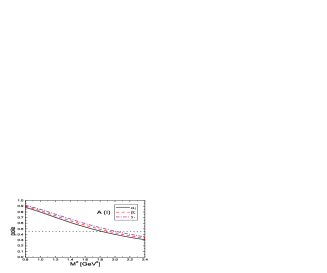
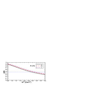
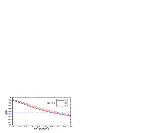
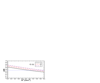
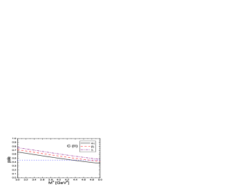
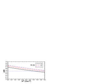
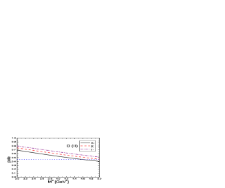
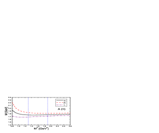
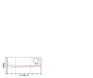
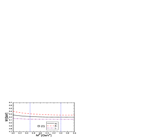
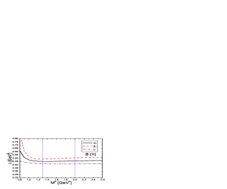
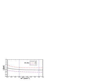
In this article, we intend to obtain the possible lowest masses, which correspond to the largest correlation lengths, and impose the two criteria of the QCD sum rules on the scalar and axial-vector heavy diquark states to choose the Borel parameter $M^{2}$ and threshold parameter $s_{0}$, i.e. we take smaller threshold parameters and Borel parameters (also Borel windows) than that presented in Table 1, and adjust them to warrant the uniform pole contributions (about $(46-71)\%$, the smallest pole contribution presented in Table 1). The preferred values are shown in Fig.1 and Table 4, where we can see explicitly that the pole contributions are about $(45-70)\%$, and the contributions from the different terms in the operator product expansion have the hierarchy: perturbative-term >⟨q¯​q⟩+⟨q¯​gs​σ​G​qβŸ©β‰«βŸ¨Ξ±s​G​GΟ€βŸ©absentdelimited-βŸ¨βŸ©Β―π‘žπ‘ždelimited-βŸ¨βŸ©Β―π‘žsubscriptπ‘”π‘ πœŽπΊπ‘žmuch-greater-thandelimited-⟨⟩subscriptπ›Όπ‘ πΊπΊπœ‹>\langle\bar{q}q\rangle+\langle\bar{q}g_{s}\sigma Gq\rangle\gg\langle\frac{\alpha_{s}GG}{\pi}\rangle, the two criteria of the QCD sum rules are well satisfied also. On the other hand, the values of the masses and pole residues are rather stable with variations of the Borel parameters in the Borel windows. In fact, we can take even smaller threshold parameters than that presented in Table 4, however, the Borel windows are too small to make reliable predictions.

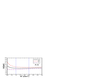
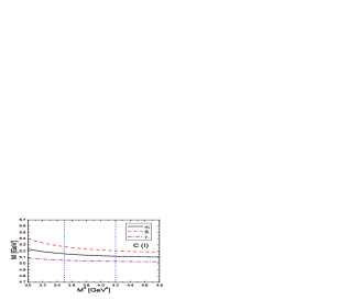
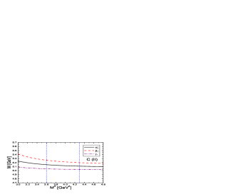
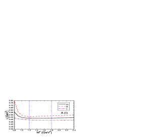
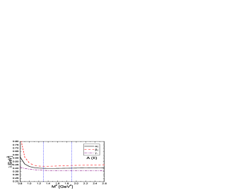
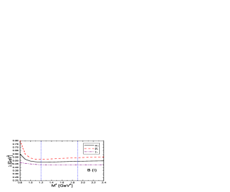
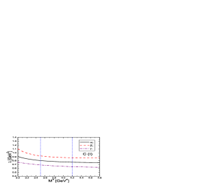
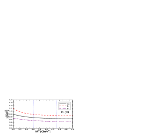
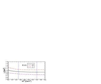
Taking into account all uncertainties of the relevant parameters, finally we obtain the (lowest) values of the masses and pole resides of the scalar and axial-vector heavy diquark states, which are shown in Figs.2-3 and Tables 2-3. In Table 2, we also present the masses from the relativistic quark model based on a quasipotential approach in QCD [35], the Bethe-Salpeter equation [36], and the constituent diquark model [29, 37, 38]. From the table, we can see that the values from different theoretical approaches differ from each other greatly, and one should be careful when using them. In Ref.[26], we introduce new QCD sum rules to study the nonet scalar mesons and take the values of the scalar diquark masses from the QCD sum rules for consistency [34].

The $SU(3)$ breaking effects for the masses of the scalar and axial-vector heavy diquark states are buried in the uncertainties. Naively, we expect the axial-vector heavy diquark states have larger masses than the corresponding scalar heavy diquark states. From Table 2, we can see that it is not the case, they have degenerate masses. Lattice QCD calculations for the light flavors indicate that the strong attraction in the scalar diquark channels favors the formation of good diquarks, the weaker attraction in the axial-vector diquark channels maybe form bad diquarks, the energy gap between the axial-vector and scalar diquarks is about $\frac{2}{3}$ of the $\Delta$-nucleon mass splitting, i.e. $\approx 0.2\,\rm{GeV}$ [44, 45], which is expected from the hypersplitting color-spin interaction $\frac{C}{m_{i}m_{j}}\vec{T}_{i}\cdot\vec{T}_{j}\vec{\sigma}_{i}\cdot\vec{\sigma}_{j}$, where the $C$ is a coefficient [2, 5]. The coupled rainbow Dyson-Schwinger equation and ladder Bethe-Salpeter equation also indicate such an energy hierarchy [46]. Comparing with the light diquark states, the contribution from the hypersplitting color-spin interaction $\frac{C}{m_{i}m_{j}}\vec{T}_{i}\cdot\vec{T}_{j}\vec{\sigma}_{i}\cdot\vec{\sigma}_{j}$ to the heavy diquark states is greatly suppressed due to the large constituent quark masses, and the scalar and axial-vector heavy diquark states have almost degenerate masses.

$M^{2}(\rm{GeV}^{2})$ $s_{0}(\rm{GeV}^{2})$ pole perturbative ⟨q¯​q⟩+⟨q¯​gs​σ​G​q⟩delimited-βŸ¨βŸ©Β―π‘žπ‘ždelimited-βŸ¨βŸ©Β―π‘žsubscriptπ‘”π‘ πœŽπΊπ‘ž\langle\bar{q}q\rangle+\langle\bar{q}g_{s}\sigma Gq\rangle ⟨αs​G​GΟ€βŸ©delimited-⟨⟩subscriptπ›Όπ‘ πΊπΊπœ‹\langle\frac{\alpha_{s}GG}{\pi}\rangle
$cq(0^{+})$ $1.2-2.2$ $5.6\pm 0.3$ $(45-86)\%$ $(59-73)\%$ $(26-40)\%$ $<1\%$
$cq(1^{+})$ $1.7-2.7$ $6.3\pm 0.3$ $(45-78)\%$ $(68-78)\%$ $(23-33)\%$ $<1\%$
$cs(0^{+})$ $1.4-2.4$ $6.1\pm 0.3$ $(46-83)\%$ $(76-85)\%$ $(15-23)\%$ $<1\%$
$cs(1^{+})$ $2.0-3.0$ $6.8\pm 0.3$ $(46-74)\%$ $(82-87)\%$ $(13-19)\%$ $<1\%$
$bq(0^{+})$ $3.8-5.3$ $33.0\pm 1.0$ $(46-76)\%$ $(64-71)\%$ $(29-36)\%$ $<1\%$
$bq(1^{+})$ $4.5-6.0$ $34.0\pm 1.0$ $(46-72)\%$ $(68-74)\%$ $(26-32)\%$ $<1\%$
$bs(0^{+})$ $4.5-6.0$ $34.5\pm 1.0$ $(46-72)\%$ $(80-84)\%$ $(16-20)\%$ $<1\%$
$bs(1^{+})$ $4.9-6.4$ $35.0\pm 1.0$ $(46-71)\%$ $(81-85)\%$ $(16-20)\%$ $<1\%$
Table 1: The Borel parameters $M^{2}$ and threshold parameters $s_{0}$ for the heavy diquark states. The ”pole” stands for the contribution from the pole term to the spectral density. The ”perturbative” stands for the contribution from the perturbative term in the operator product expansion, etc, where the central value of the threshold parameter $s_{0}$ is taken. The contributions from the $\langle\bar{q}q\rangle$ and ⟨q¯​gs​σ​G​q⟩delimited-βŸ¨βŸ©Β―π‘žsubscriptπ‘”π‘ πœŽπΊπ‘ž\langle\bar{q}g_{s}\sigma Gq\rangle are not shown independently for simplicity, and ⟨q¯​qβŸ©β‰«βŸ¨q¯​gs​σ​G​q⟩much-greater-thandelimited-βŸ¨βŸ©Β―π‘žπ‘ždelimited-βŸ¨βŸ©Β―π‘žsubscriptπ‘”π‘ πœŽπΊπ‘ž\langle\bar{q}q\rangle\gg\langle\bar{q}g_{s}\sigma Gq\rangle.
$\widehat{M}$ $M$ Ref.[35] Refs.[29, 37, 38] Ref.[36] Ref.[16]
$cq(0^{+})$ $1.86\pm 0.10$ $1.77\pm 0.08$ 1.793 1.933 2.088 1.867 $[D]$
$cq(1^{+})$ $1.96\pm 0.10$ $1.76\pm 0.08$ 2.036 2.067 2.009 $[D^{*}]$
$cs(0^{+})$ $1.98\pm 0.10$ $1.84\pm 0.08$ 2.091 1.955 2.192 1.969 $[D_{s}]$
$cs(1^{+})$ $2.08\pm 0.09$ $1.84\pm 0.08$ 2.158 2.168 2.112 $[D^{*}_{s}]$
$bq(0^{+})$ $5.23\pm 0.09$ $5.14\pm 0.12$ 5.359 5.267 5.556 5.279 $[B]$
$bq(1^{+})$ $5.28\pm 0.09$ $5.13\pm 0.11$ 5.381 5.539 5.325 $[B^{*}]$
$bs(0^{+})$ $5.35\pm 0.09$ $5.20\pm 0.07$ 5.462 5.648 5.366 $[B_{s}]$
$bs(1^{+})$ $5.38\pm 0.09$ $5.20\pm 0.08$ 5.482 5.636 5.415 $[B^{*}_{s}]$
Table 2: The masses $M$ of the scalar and axial-vector heavy diquark states, the values are in unit of $\rm{GeV}$, the wide-hat denotes the values from the parameters presented in Table 1.
$\widehat{\lambda}$ $\lambda$
$cq(0^{+})$ $0.53\pm 0.08$ $0.43\pm 0.05$
$cq(1^{+})$ $0.57\pm 0.08$ $0.40\pm 0.04$
$cs(0^{+})$ $0.64\pm 0.09$ $0.48\pm 0.05$
$cs(1^{+})$ $0.69\pm 0.08$ $0.45\pm 0.05$
$bq(0^{+})$ $1.02\pm 0.14$ $0.78\pm 0.14$
$bq(1^{+})$ $1.08\pm 0.14$ $0.76\pm 0.12$
$bs(0^{+})$ $1.27\pm 0.17$ $0.91\pm 0.14$
$bs(1^{+})$ $1.28\pm 0.17$ $0.88\pm 0.14$
Table 3: The pole residues $\lambda$ of the scalar and axial-vector heavy diquark states, the values are in unit of $\rm{GeV}^{2}$, the wide-hat denotes the values from the parameters presented in Table 1.
$M^{2}(\rm{GeV}^{2})$ $s_{0}(\rm{GeV}^{2})$ pole perturbative ⟨q¯​q⟩+⟨q¯​gs​σ​G​q⟩delimited-βŸ¨βŸ©Β―π‘žπ‘ždelimited-βŸ¨βŸ©Β―π‘žsubscriptπ‘”π‘ πœŽπΊπ‘ž\langle\bar{q}q\rangle+\langle\bar{q}g_{s}\sigma Gq\rangle ⟨αs​G​GΟ€βŸ©delimited-⟨⟩subscriptπ›Όπ‘ πΊπΊπœ‹\langle\frac{\alpha_{s}GG}{\pi}\rangle
$cq(0^{+})$ $1.2-1.8$ $4.8\pm 0.2$ $(46-76)\%$ $(54-62)\%$ $(37-45)\%$ $<1\%$
$cq(1^{+})$ $1.3-1.9$ $4.8\pm 0.2$ $(47-75)\%$ $(53-60)\%$ $(42-50)\%$ $<3\%$
$cs(0^{+})$ $1.2-1.9$ $5.0\pm 0.2$ $(45-77)\%$ $(69-76)\%$ $(23-30)\%$ $<1\%$
$cs(1^{+})$ $1.3-2.0$ $5.0\pm 0.2$ $(46-76)\%$ $(68-74)\%$ $(27-34)\%$ $<2\%$
$bq(0^{+})$ $3.5-4.2$ $30.0\pm 1.0$ $(45-67)\%$ $(53-55)\%$ $(45-47)\%$ $<1\%$
$bq(1^{+})$ $3.6-4.3$ $30.0\pm 1.0$ $(46-67)\%$ $(52-54)\%$ $(46-49)\%$ $<1\%$
$bs(0^{+})$ $3.5-4.4$ $31.0\pm 1.0$ $(46-71)\%$ $(71-73)\%$ $(27-29)\%$ $<1\%$
$bs(1^{+})$ $3.6-4.6$ $31.0\pm 1.0$ $(45-71)\%$ $(70-72)\%$ $(28-31)\%$ $<1\%$
Table 4: The preferred Borel parameters $M^{2}$ and threshold parameters $s_{0}$ for the heavy diquark states. The ”pole” stands for the contribution from the pole term to the spectral density. The ”perturbative” stands for the contribution from the perturbative term in the operator product expansion, etc, where the central value of the threshold parameter $s_{0}$ is taken. The contributions from the $\langle\bar{q}q\rangle$ and ⟨q¯​gs​σ​G​q⟩delimited-βŸ¨βŸ©Β―π‘žsubscriptπ‘”π‘ πœŽπΊπ‘ž\langle\bar{q}g_{s}\sigma Gq\rangle are not shown independently for simplicity, and ⟨q¯​qβŸ©β‰«βŸ¨q¯​gs​σ​G​q⟩much-greater-thandelimited-βŸ¨βŸ©Β―π‘žπ‘ždelimited-βŸ¨βŸ©Β―π‘žsubscriptπ‘”π‘ πœŽπΊπ‘ž\langle\bar{q}q\rangle\gg\langle\bar{q}g_{s}\sigma Gq\rangle.
Refer to caption
Refer to caption
Refer to caption
Refer to caption
Refer to caption
Refer to caption
Refer to caption
Refer to caption
Figure 1: The contributions of the pole terms to the spectral densities with variation of the Borel parameter $M^{2}$. The $A$, $B$, $C$ and $D$ denote the channels $cq$, $cs$, $bq$ and $bs$ respectively. The $\beta$ corresponds to the central values of the threshold parameters, the energy gaps among $\alpha$, $\beta$ and $\gamma$ are $0.2\,\rm{GeV}$ and $1.0\,\rm{GeV}$ for the charmed and bottom diquark states respectively. The (I) and (II) denote the scalar and axial-vector diquark states respectively.
Refer to caption
Refer to caption
Refer to caption
Refer to caption
Refer to caption
Refer to caption
Refer to caption
Refer to caption
Figure 2: The values of the diquark masses with variation of the Borel parameter $M^{2}$. The $A$, $B$, $C$ and $D$ denote the channels $cq$, $cs$, $bq$ and $bs$ respectively. The $\alpha$, $\beta$ and $\gamma$ denote the upper bound, the central value and the lower bound respectively. The (I) and (II) denote the scalar and axial-vector diquark states respectively.
Refer to caption
Refer to caption
Refer to caption
Refer to caption
Refer to caption
Refer to caption
Refer to caption
Refer to caption
Figure 3: The values of the pole residues with variation of the Borel parameter $M^{2}$. The $A$, $B$, $C$ and $D$ denote the channels $cq$, $cs$, $bq$ and $bs$ respectively. The $\alpha$, $\beta$ and $\gamma$ denote the upper bound, the central value and the lower bound respectively. The (I) and (II) denote the scalar and axial-vector diquark states respectively.

4 Conclusion

In this article, we study the mass spectrum of the scalar and axial-vector heavy diquark states with the QCD sum rules in a systematic way. The diquark masses are basic parameters in studying the tetraquark states, once reasonable values are obtained, we can study the new charmonium-like states as the tetraquark states with the new QCD sum rules developed in our previous work.

Acknowledgment

This work is supported by National Natural Science Foundation of China, Grant Numbers 10775051, 11075053, and Program for New Century Excellent Talents in University, Grant Number NCET-07-0282, and the Fundamental Research Funds for the Central Universities.

References

  • [1] M. Huang, Int. J. Mod. Phys. E14 (2005) 675.
  • [2] A. De Rujula, H. Georgi and S. L. Glashow, Phys. Rev. D12 (1975) 147; R. L. Jaffe, hep-ph/0001123.
  • [3] T. Schafer, E. V. Shuryak and J. J. M. Verbaarschot, Nucl. Phys. B412 (1994) 143.
  • [4] M. Anselmino, E. Predazzi, S. Ekelin, S. Fredriksson and D. B. Lichtenberg, Rev. Mod. Phys. 65 (1993) 1199.
  • [5] R. L. Jaffe, Phys. Rept. 409 (2005) 1.
  • [6] M. G. Alford, A. Schmitt, K. Rajagopal and T. Schafer, Rev. Mod. Phys. 80 (2008) 1455.
  • [7] D. B. Lichtenberg and L. J. Tassie, Phys. Rev. 155 (1967) 1601.
  • [8] M. Neubert and B. Stech, Phys. Lett. B231 (1989) 477; Phys. Rev. D44 (1991) 775.
  • [9] F. E. Close and A. W. Thomas, Phys. Lett. B212 (1988) 227.
  • [10] M. G. Alford, K. Rajagopal and F. Wilczek, Phys. Lett. B422 (1998) 247; R. Rapp, T. Schafer, E. V. Shuryak and M. Velkovsky, Phys. Rev. Lett. 81 (1998) 53.
  • [11] R. L. Jaffe, Phys. Rev. D15 (1977) 267; Phys. Rev. D15 (1977) 281.
  • [12] A. Selem and F. Wilczek, hep-ph/0602128; T. Friedmann, arXiv:0910.2229.
  • [13] F. E. Close and N. A. Tornqvist, J. Phys. G28 (2002) R249.
  • [14] C. Amsler and N. A. Tornqvist, Phys. Rept. 389 (2004) 61.
  • [15] J. Weinstein and N. Isgur, Phys. Rev. Lett. 48 (1982) 659; F. E. Close, N. Isgur and S. Kumana, Nucl. Phys. B389 (1993) 513; N. N. Achasov, V. V. Gubin and V. I. Shevchenko, Phys. Rev. D56 (1997) 203.
  • [16] C. Amsler et al, Phys. Lett. B667 (2008) 1.
  • [17] E. M. Aitala et al, Phys. Rev. Lett. 89 (2002) 121801.
  • [18] M. Ablikim et al, Phys. Lett. B633 (2006) 681.
  • [19] M. Ablikim et al, arXiv:1008.4489.
  • [20] M. A. Shifman, A. I. Vainshtein and V. I. Zakharov, Nucl. Phys. B147 (1979) 385, 448.
  • [21] L. J. Reinders, H. Rubinstein and S. Yazaki, Phys. Rept. 127 (1985) 1.
  • [22] R. D. Matheus and S. Narison, Nucl. Phys. Proc. Suppl. 152 (2006) 236; Z. G. Wang, S. L. Wan and W. M. Yang, Eur. Phys. J. C45 (2006) 201; Z. G. Wang, W. M. Yang and S. L. Wan, J. Phys. G31 (2005) 971; H. X. Chen, A. Hosaka and S. L. Zhu, Phys. Rev. D76 (2007) 094025; Z. G. Wang, Nucl. Phys. A791 (2007) 106.
  • [23] Z. G. Wang, Eur. Phys. J. C62 (2009) 375; Phys. Rev. D79 (2009) 094027; J. Phys. G36 (2009) 085002; Eur. Phys. J. C63 (2009) 115; Eur. Phys. J. C67 (2010) 411; Z. G. Wang and X. H. Zhang, Eur. Phys. J. C66 (2010) 419; Commun. Theor. Phys. 54 (2010) 323.
  • [24] R. D. Matheus, S. Narison, M. Nielsen and J. M. Richard, Phys. Rev. D75 (2007) 014005; S. H. Lee, A. Mihara, F. S. Navarra and M. Nielsen, Phys. Lett. B661 (2008) 28.
  • [25] Z. G. Wang, Eur. Phys. J. C70 (2010) 139.
  • [26] Z. G. Wang, arXiv:1008.0974.
  • [27] N. Drenska, R. Faccini, F. Piccinini, A. Polosa, F. Renga and C. Sabelli, arXiv:1006.2741; E. S. Swanson, Phys. Rept. 429 (2006) 243; E. Klempt and A. Zaitsev, Phys. Rept. 454 (2007) 1; M. B. Voloshin, Prog. Part. Nucl. Phys. 61 (2008) 455; S. Godfrey and S. L. Olsen, Ann. Rev. Nucl. Part. Sci. 58 (2008) 51.
  • [28] S. K. Choi et al, Phys. Rev. Lett. 91 (2003) 262001; V. M. Abazov et al, Phys. Rev. Lett. 93 (2004) 162002; D. E. Acosta et al, Phys. Rev. Lett. 93 (2004) 072001.
  • [29] L. Maiani, F. Piccinini, A. D. Polosa and V. Riquer, Phys. Rev. D71 (2005) 014028.
  • [30] S. K. Choi et al, Phys. Rev. Lett. 100 (2008) 142001.
  • [31] R. Mizuk et al, Phys. Rev. D80 (2009) 031104.
  • [32] R. Mizuk et al, Phys. Rev. D78 (2008) 072004.
  • [33] H. G. Dosch, M. Jamin and B. Stech, Z. Phys. C42 (1989) 167; M. Jamin and M. Neubert, Phys. Lett. B238 (1990) 387.
  • [34] A. Zhang, T. Huang and T. G. Steele, Phys. Rev. D76 (2007) 036004.
  • [35] D. Ebert, R. N. Faustov and V. O. Galkin, Phys. Lett. B634 (2006) 214; Mod. Phys. Lett. A24 (2009) 567.
  • [36] Y. M. Yu et al, Commun. Theor. Phys. 46 (2006) 1031.
  • [37] N. V. Drenska, R. Faccini and A. D. Polosa, Phys. Rev. D79 (2009) 077502.
  • [38] A. Ali, C. Hambrock, I. Ahmed and M. J. Aslam, Phys. Lett. B684 (2010) 28.
  • [39] B. L. Ioffe, Prog. Part. Nucl. Phys. 56 (2006) 232.
  • [40] S. Narison, Camb. Monogr. Part. Phys. Nucl. Phys. Cosmol. 17 (2002) 1.
  • [41] A. Khodjamirian and R. Ruckl, Adv. Ser. Direct. High Energy Phys. 15 (1998) 345.
  • [42] Z. G. Wang, Eur. Phys. J. A45 (2010) 267; Eur. Phys. J. C68 (2010) 459; Phys. Lett. B685 (2010) 59; Eur. Phys. J. C68 (2010) 479; arXiv:1003.2838.
  • [43] C. J. Burden, L. Qian, C. D. Roberts, P. C. Tandy and M. J. Thomson, Phys. Rev. C55 (1997) 2649; A. Bender, C. D. Roberts and L. v. Smekal, Phys. Lett. B380 (1996) 7.
  • [44] C. Alexandrou, P. de Forcrand and B. Lucini, Phys. Rev. Lett. 97 (2006) 222002.
  • [45] M. Hess, F. Karsch, E. Laermann and I. Wetzorke, Phys. Rev. D58 (1998) 111502.
  • [46] P. Maris, Few Body Syst. 32 (2002) 41.