Triaxial quadrupole deformation dynamics in $sd$-shell nuclei around ²⁶Mg

Abstract

Large-amplitude dynamics of axial and triaxial quadrupole deformation in ^24,26Mg, ²⁴Ne, and ²⁸Si is investigated on the basis of the quadrupole collective Hamiltonian constructed with use of the constrained Hartree-Fock-Bogoliubov plus the local quasiparticle random-phase approximation method. The calculation reproduces well properties of the ground rotational bands, and $\beta$ and $\gamma$ vibrations in ²⁴Mg and ²⁸Si. The $\gamma$-softness in the collective states of ²⁶Mg and ²⁴Ne are discussed. Contributions of the neutrons and protons to the transition properties are also analyzed in connection with the large-amplitude quadrupole dynamics.

I Introduction

It is known that collective deformation grows up in the middle of the $sd$-shell region. The appearance of the prolate ground state of ²⁴Mg and the oblate ground state of ²⁸Si Horikawa et al. (1971); Ball et al. (1980); Gupta and Harvey (1967); Ragnarsson and Nilsson (1970) is associated with the shell gaps $N=Z=12$ at the prolate region and $N=Z=14$ at the oblate region in Nilsson diagram Bohr and Mottelson (1998a), respectively. Because of the shell gaps in the deformed regions, various shapes are expected to appear in the mass number region around ²⁴Mg and ²⁸Si.

Moreover, triaxial deformation degree of freedom plays very important roles on the low-lying collective dynamics in this mass region Kurath (1972). In ²⁴Mg, possibility of the triaxial deformation in the ground states has been discussed for decades Koepf and Ring (1988); Bonche et al. (1987); Sheline et al. (1988). The low-lying $K=2$ band built on top of the $2_{2}^{+}$ state suggests that the triaxial degree of freedom is activated in the collective dynamics. In ²⁸Si, importance of triaxiality has been suggested in connection with the large-amplitude collective dynamics of the oblate-prolate shape coexistence Walet et al. (1991); Pelet and Letourneux (1977).

In contrast to the well-developed deformations in ²⁴Mg and ²⁸Si, the deformation property of ²⁶Mg is not yet fully clarified. Since it is a system with $N=14$ and $Z=12$, neutrons and protons favor different shapes separately. Indeed, so far many mean-field calculations with use of the realistic effective interactions have been performed for ²⁶Mg within an axial symmetry restriction, and they yielded a coexistence of oblate and prolate shapes with an oblate minimum Rodríguez-Guzmán et al. (2002); Péru and Goutte (2008); Terasaki et al. (1997). On the other hand, the symmetry-unrestricted mean-field calculations using a Skyrme density functional (SkM*) Inakura or relativistic model Yao et al. (2011) show extremely triaxially soft potential energy surfaces.

In the study of collective excitations in this mass region, the quasiparticle random-phase approximation (QRPA) calculations have been systematically performed by employing various effective interactions Péru and Goutte (2008); Yoshida and Giai (2008); Losa et al. (2010). The QRPA is a standard tool to analyze the collective modes of excitations. However, in order to discuss the low-lying collective dynamics of nuclei which are very soft against quadrupole deformation, one should use a microscopic theory of large-amplitude collective motion instead of the small-amplitude theory such as the QRPA. The generator coordinate method (GCM) with the restriction of axial symmetry Rodríguez-Guzmán et al. (2002), and the antisymmetrized molecular dynamics + multi-configuration mixing Taniguchi et al. (2009) have been performed using the energy density functionals for magnesium isotopes and ²⁸Si, respectively. However, ²⁶Mg is soft against $\beta$ and $\gamma$ directions as shown in the potential energy surface Rodríguez-Guzmán et al. (2002); Péru and Goutte (2008); Terasaki et al. (1997); Inakura , and therefore the triaxial degree of freedom in addition to the axial degree of freedom should be included for the description of the low-lying collective dynamics.

Quite recently, the GCM calculations including axial and triaxial generator coordinates have been performed Bender and Heenen (2008); Rodríguez and Egido (2010); Yao et al. (2010, 2011) for magnesium isotopes. The first applications are concentrated on the low-lying states of ²⁴Mg, in which the small-amplitude description in the prolate mean field is rather good. In Ref. Yao et al. (2011), the properties of the yrast states of the magnesium isotopes are discussed systematically.

The quadrupole collective Hamiltonian provides a powerful theoretical tool to investigate the large-amplitude collective motion while taking into account the $\beta$ and $\gamma$ degrees of freedom Bohr and Mottelson (1998a); Kumar and Baranger (1967); Belyaev (1965); Próchniak and Rohoziński (2009). Recently, on the basis of the adiabatic self-consistent collective coordinate method Matsuo et al. (2000); Hinohara et al. (2007), a new microscopic method to construct the collective Hamiltonian has been developed, called the constrained Hartree-Fock-Bogoliubov plus local QRPA (CHFB+LQRPA) Hinohara et al. (2010). In this method, the collective potential is calculated by the CHFB equation, while the inertial functions for large-amplitude quadrupole shape vibration and the three-dimensional rotation are determined from the normal modes on the CHFB state in $(\beta,\gamma)$ plane. A new point of this method is that the contributions from the time-odd mean field are taken into account in evaluating the vibrational and rotational inertial masses. So far this CHFB + LQRPA method in conjunction with the pairing-plus-quadrupole (P+Q) model Baranger and Kumar (1968); Bes and Sorensen (1969) including the quadrupole-pairing force has been successfully applied to the oblate-prolate shape coexistence in proton-rich Se and Kr isotopes Hinohara et al. (2010); Sato and Hinohara (2011).

In this paper, we analyze the role of triaxiality in connection with the large-amplitude collective motion in the low-lying states of ²⁴Mg, ²⁸Si, ²⁶Mg, and ²⁴Ne using the quadrupole collective Hamiltonian calculated by use of the CHFB + LQRPA method with the P+Q model. We also discuss the roles of neutrons and protons in $N\neq Z$ nuclei on the large-amplitude collective dynamics in relation to the electric transition properties. This article is organized as follows. In the next section, the formulation of the CHFB+LQRPA method is briefly recapitulated. The results of the numerical calculations are presented in Sec. III, and the role of the triaxial degree of freedom in these nuclei is discussed in Sec. IV. Summary is given in Sec. V.

II Formulation

II.1 CHFB+LQRPA method

The theoretical approach, the CHFB + LQRPA method is briefly summarized in this section. See Ref. Hinohara et al. (2010) for detailed description of the method.

The method enables us to derive the five-dimensional quadrupole collective Hamiltonian of the Bohr-Mottelson type Bohr and Mottelson (1998a); Kumar and Baranger (1967); Belyaev (1965); Próchniak and Rohoziński (2009)

$${\cal H}_{\rm coll}= T_{\rm vib}+T_{\rm rot}+V(\beta,\gamma),$$ (1)

$$T_{\rm vib}= \frac{1}{2}D_{\beta\beta}(\beta,\gamma)\dot{\beta}^{2}+D_{\beta\gamma}(\beta,\gamma)\dot{\beta}\dot{\gamma}+\frac{1}{2}D_{\gamma\gamma}(\beta,\gamma)\dot{\gamma}^{2},$$ (2)

$$T_{\rm rot}= \frac{1}{2}\sum_{k=1}^{3}{\cal J}_{k}(\beta,\gamma)\omega^{2}_{k},$$ (3)

where $V(\beta,\gamma)$ is the collective potential in the $(\beta,\gamma)$ plane. The quantities $T_{\rm vib}$ and $T_{\rm rot}$ are the vibrational and rotational kinetic energies. The inertial functions $D_{\beta\beta},D_{\gamma\gamma}$, and $D_{\beta\gamma}$ are the vibrational masses associated with the time-derivatives of the two quadrupole deformation variables, $\dot{\beta}$ and $\dot{\gamma}$, and ${\cal J}_{k}$ are the rotational moments of inertia associated with the three components of the rotational angular velocities $\omega_{k}$ defined with respect to the principal axes.

The collective potential and the inertial functions in the collective Hamiltonian (1) are determined microscopically in the CHFB + LQRPA method. The collective potential is determined by solving the CHFB equation

$$\left\langle\phi(\beta,\gamma)\right|\hat{H}_{\rm CHFB}(\beta,\gamma)\left|\phi(\beta,\gamma)\right\rangle=0,$$ (4)

where the CHFB Hamiltonian is given as

$$\hat{H}_{\rm CHFB}=\hat{H}-\sum_{\tau=n,p}\lambda^{(\tau)}(\beta,\gamma)\widetilde{N}^{(\tau)}-\sum_{m=0,2}\mu_{m}(\beta,\gamma)\hat{D}_{2m}^{(+)},$$ (5)

with the constraints on particle numbers and quadrupole deformations. Here $\hat{H}$ is the microscopic Hamiltonian, $\left|\phi(\beta,\gamma)\right\rangle$ is the CHFB state, $\lambda^{(\tau)}(\beta,\gamma)$ and $\mu_{m}(\beta,\gamma)$ are the Lagrange multipliers, $\widetilde{N}^{(\tau)}\equiv\hat{N}^{(\tau)}-N_{0}^{(\tau)}$ are the particle number operators measured from $N_{0}^{(\tau)}$ which are the neutron and proton particle numbers of the nucleus. The operators $\hat{D}^{(+)}_{2m}$ are the Hermitian part of the quadrupole operators given by $\hat{D}^{(+)}_{2m}\equiv(\hat{D}_{2m}+\hat{D}_{2-m})/2$. The collective potential is given by

$$V(\beta,\gamma)=\left\langle\phi(\beta,\gamma)\right|\hat{H}\left|\phi(\beta,\gamma)\right\rangle.$$ (6)

On top of the CHFB state, the local normal modes are calculated by solving the LQRPA equations

$$\delta\left\langle\phi(\beta,\gamma)\right|[\hat{H}_{\rm CHFB}(\beta,\gamma),\hat{Q}^{i}(\beta,\gamma)]\\ -\frac{1}{i}\hat{P}_{i}(\beta,\gamma)\left|\phi(\beta,\gamma)\right\rangle=0,$$ (7)

$$\delta\left\langle\phi(\beta,\gamma)\right|\left[\hat{H}_{\rm CHFB}(\beta,\gamma),\frac{1}{i}\hat{P}_{i}(\beta,\gamma)\right]\\ -C_{i}(\beta,\gamma)\hat{Q}^{i}(\beta,\gamma)\left|\phi(\beta,\gamma)\right\rangle=0.$$ (8)

Here $\hat{Q}^{i}(\beta,\gamma)$ and $\hat{P}_{i}(\beta,\gamma)$ are the infinitesimal generators locally defined as functions of $(\beta,\gamma)$. The quantity $C_{i}(\beta,\gamma)=\omega^{2}_{i}(\beta,\gamma)$ is the squared eigen frequency of the normal mode. We choose two collective modes from the LQRPA modes, following the minimal metric criterion in Ref. Hinohara et al. (2010). The vibrational masses $D_{\beta\beta},D_{\gamma\gamma}$, and $D_{\beta\gamma}$ are determined from the transformation of the collective coordinates spanned by the two LQRPA modes into $(\beta,\gamma)$.

The rotational moments of inertia are calculated by solving the LQRPA equations for rotation on top of the CHFB state.

$$\delta\left\langle\phi(\beta,\gamma)\right|[\hat{H}_{\rm CHFB},\hat{\Psi}_{k}(\beta,\gamma)]-\frac{1}{i}({\cal J}_{k})^{-1}\hat{I}_{k}\left|\phi(\beta,\gamma)\right\rangle=0,$$ (9)

$$\left\langle\phi(\beta,\gamma)\right|[\hat{\Psi}_{k}(\beta,\gamma),\hat{I}_{k^{\prime}}]\left|\phi(\beta,\gamma)\right\rangle=i\delta_{kk^{\prime}},$$ (10)

where $\hat{\Psi}_{k}(\beta,\gamma)$ and $\hat{I}_{k}$ represent the rotational angles and the angular momentum operators with respect to the three principal axes associated with the CHFB state $\left|\phi(\beta,\gamma)\right\rangle$, and ${\cal J}_{k}$ are the LQRPA moments of inertia.

Pauli’s prescription is used to quantize the classical collective Hamiltonian (1). From the solution of the collective Schrödinger equation

$$\left\{\hat{T}_{\rm vib}+\hat{T}_{\rm rot}+V(\beta,\gamma)\right\}\Psi_{\alpha IM}(\beta,\gamma,\Omega)=E_{\alpha I}\Psi_{\alpha IM}(\beta,\gamma,\Omega),$$ (11)

we obtain the collective wave function $\Psi_{\alpha IM}(\beta,\gamma,\Omega)$ as functions of quadrupole deformations $(\beta,\gamma)$ and three Euler angles $\Omega$. The collective wave function is specified by the angular momentum $I$, and its projection onto the $z$-axis of the laboratory frame, $M$, and $\alpha$ distinguishes the states which have the same $I$ and $M$.

The collective wave function is written in the following form

$$\Psi_{\alpha IM}(\beta,\gamma,\Omega)=\sum_{K\geq 0,{\rm even}}\Phi_{\alpha IK}(\beta,\gamma)\langle\Omega|IMK\rangle,$$ (12)

where $\Phi_{\alpha IK}(\beta,\gamma)$ is the vibrational part of the collective wave function, and the rotational part is written as

$$\langle\Omega|IMK\rangle=\sqrt{\frac{2I+1}{16\pi^{2}(1+\delta_{k0})}}[D^{I}_{MK}(\Omega)+(-)^{I}D^{I}_{M-K}(\Omega)].$$ (13)

Here $D^{I}_{MK}$ is the Wigner’s rotation matrix and $K$ is the projection of the angular momentum onto the $z$-axis in the body-fixed frame.

The vibrational wave functions are normalized as

$$\int d\beta d\gamma|\Phi_{\alpha I}(\beta,\gamma)|^{2}|G(\beta,\gamma)|^{\frac{1}{2}}=1,$$ (14)

where

$$|\Phi_{\alpha I}(\beta,\gamma)|^{2}\equiv\sum_{K\geq 0,{\rm even}}|\Phi_{\alpha IK}(\beta,\gamma)|^{2},$$ (15)

and the volume element $|G(\beta,\gamma)|^{\frac{1}{2}}d\beta d\gamma$ is given by

$$|G(\beta,\gamma)|^{\frac{1}{2}}d\beta d\gamma=2\beta^{4}\sqrt{W(\beta,\gamma)R(\beta,\gamma)}\sin 3\gamma d\beta d\gamma,$$ (16)

$$W(\beta,\gamma)= \{D_{\beta\beta}(\beta,\gamma)D_{\gamma\gamma}(\beta,\gamma)-[D_{\beta\gamma}(\beta,\gamma)]^{2}\}\beta^{-2},$$ (17)

$$R(\beta,\gamma)= D_{1}(\beta,\gamma)D_{2}(\beta,\gamma)D_{3}(\beta,\gamma),$$ (18)

where $D_{k}(\beta,\gamma)$ are related to the moments of inertia as ${\cal J}_{k}(\beta,\gamma)=4\beta^{2}D_{k}(\beta,\gamma)\sin^{2}(\gamma-2\pi k/3)$.

The requantization form, the symmetries, and boundary conditions of the collective Hamiltonian are described in Ref. Kumar and Baranger (1967).

The electric properties are calculated following the discussions in Refs. Kumar and Baranger (1967); Sato and Hinohara (2011). The value of $B(E2)$ and the spectroscopic quadrupole moment are given by

$$B(E2;\alpha I\rightarrow\alpha^{\prime}I^{\prime})=(2I+1)^{-1}|\langle\alpha I||\hat{D}^{{}^{\prime}(E2)}||\alpha^{\prime}I^{\prime}\rangle|^{2},$$ (19)

and

$$Q(\alpha I)=\sqrt{\frac{16\pi}{5}}\begin{pmatrix}I&2&I\\ -I&0&I\end{pmatrix}\langle\alpha I||\hat{D}^{{}^{\prime}(E2)}||\alpha I\rangle.$$ (20)

The reduced matrix element in Eqs. (19) and (20) is calculated as

$$\langle\alpha I||\hat{D}^{{}^{\prime}(E2)}||\alpha^{\prime}I^{\prime}\rangle=\int d\beta d\gamma|G(\beta,\gamma)|^{\frac{1}{2}}\rho^{(E2)}_{\alpha I\alpha^{\prime}I^{\prime}}(\beta,\gamma),$$ (21)

$$\rho^{(E2)}_{\alpha I\alpha^{\prime}I^{\prime}} (\beta,\gamma)=\sqrt{(2I+1)(2I^{\prime}+1)}(-)^{I}$$

$$\sum_{K\geq 0,{\rm even}}\left\{\begin{pmatrix}I&2&I^{\prime}\\ -K&0&K\end{pmatrix}\Phi_{\alpha,I,K}D^{(E2)}_{0+}\Phi_{\alpha^{\prime},I^{\prime},K^{\prime}}\right.$$

$$+\sqrt{1+\delta_{K0}} \left.\left[\left\{\begin{pmatrix}I&2&I^{\prime}\\ -K-2&2&K\end{pmatrix}\Phi_{\alpha,I,K+2}D^{(E2)}_{2+}\Phi_{\alpha^{\prime},I^{\prime},K}\right.\right.\right.$$

$$+(-)^{I+I^{\prime}} \left.\left.\begin{pmatrix}I&2&I^{\prime}\\ K&2&-K-2\end{pmatrix}\Phi_{\alpha,I,K}D^{(E2)}_{2+}\Phi_{\alpha^{\prime},I^{\prime},K+2}\right]\right\}$$ (22)

where $\rho^{(E2)}_{\alpha,I,\alpha^{\prime},I^{\prime}}(\beta,\gamma)$ is the $E2$ transition density. The quantities $D^{(E2)}_{m+}(\beta,\gamma)$ are the expectation values of the $E2$ operator in the intrinsic frame,

$$D^{(E2)}_{m+}(\beta,\gamma)=\left\langle\phi(\beta,\gamma)\right|\sum_{\tau=n,p}e_{\rm eff}^{(\tau)}\hat{D}_{m+}^{(\tau)}\left|\phi(\beta,\gamma)\right\rangle,$$ (23)

where $e_{\rm eff}^{(\tau)}$ are the neutron and proton effective charges, and $\hat{D}_{m+}^{(\tau)}\equiv(\hat{D}_{m}^{(\tau)}+\hat{D}_{-m}^{(\tau)})/2$ are the neutron and proton parts of the quadrupole operators.

II.2 Model Hamiltonian and parameters

The pairing-plus-quadrupole model Bes and Sorensen (1969); Baranger and Kumar (1968) including the quadrupole-pairing interaction is adopted as a microscopic Hamiltonian in the present work. The single-particle model space consists of harmonic oscillator two-major shells ($p$-shell and $sd$-shell) both for neutrons and protons. The modified oscillator values are used as the spherical single-particle energies Nilsson and Ragnarsson (1995). The values of the neutron and proton monopole pairing strengths and the quadrupole particle-hole interaction strengths are summarized in Table 1. The strength of the quadrupole-pairing interaction is evaluated at the spherical CHFB state with use of the prescription proposed by Sakamoto and Kishimoto Sakamoto and Kishimoto (1990). The interaction strengths of ²⁴Mg are adjusted to reproduce the quadrupole deformation of the prolate potential minimum and the pairing energy at spherical shape of ²⁴Mg calculated with Skyrme SkM* density functional and the mixed surface-volume type pairing functional in Ref. Losa et al. (2010). A simple mass number dependence of the interaction strengths is used to obtain those for ²⁶Mg, ²⁴Ne, and ²⁸Si. Only the quadrupole strength for ²⁸Si is increased in order to adjust the deformation of the oblate HFB minimum.

The Fock term is neglected following the conventional prescription of the P+Q model. Therefore we call the present framework Hartree-Bogoliubov (HB) instead of Hartree-Fock-Bogoliubov (HFB). Following Baranger and Kumar Baranger and Kumar (1968), the reduction factors are multiplied by the quadrupole matrix elements between the single-particle states in the upper shells, and the nuclear radial parameter $R=1.2A^{1/3}$ fm is used in the calculation of the harmonic oscillator length $b$. In the calculation of $E2$ transition strengths and quadrupole moments, the quadrupole operator without reduction factor is used Baranger and Kumar (1968), and the nuclear radial parameter with the higher order $A$-dependence $R=1.12A^{1/3}(1+3.84A^{-2/3})^{1/2}$ fm Bohr and Mottelson (1998b) is adopted to quantitatively evaluate $E2$ matrix elements.

The two-dimensional mesh in the $\beta$ and $\gamma$ directions is used to express the collective Hamiltonian in the ($\beta,\gamma$) plane. The 60 mesh points are taken both in the range $0<\beta<\beta_{\rm max}$ and $0^{\circ}<\gamma<60^{\circ}$. As for $\beta_{\rm max}$, 0.6 is used as common value, except $\beta_{\rm max}=0.5$ used for ²⁸Si, because we could not get converged solution which satisfies the CHB equation with four constraints at large deformation $\beta>0.5$ near the prolate region in ²⁸Si.

Table 1: Neutron and proton monopole pairing interaction strengths $G_{0}^{(\tau)}$ and quadrupole particle-hole interaction strength $\chi^{\prime}=\chi b^{4}.$

	$G_{0}^{(n)}$ (MeV)	$G_{0}^{(p)}$ (MeV)	$\chi^{\prime}$ (MeV)
24Mg	0.79	0.83	1.56
26Mg	0.73	0.77	1.37
24Ne	0.79	0.83	1.56
28Si	0.68	0.71	1.30

III Results

III.1 Collective potentials

The collective potentials calculated for $N=Z$ nuclei, ²⁴Mg and ²⁸Si, are shown in Figs. 1 and 2. The collective potential of ²⁴Mg shows a prolate minimum at $\beta\sim 0.41$, while that of ²⁸Si shows an oblate minimum at $\beta\sim 0.26$. As shown in Fig. 3, deformed shell gaps are found at prolately and oblately deformed regions in the present model. It corresponds to the appearance of the deformed minima in the collective potentials of ²⁴Mg and ²⁸Si. In ²⁴Mg, the triaxial potential valley from the prolate minimum to the oblate region exists in the small deformed region with $\beta\sim 0.2$. In ²⁸Si, the collective potential curve around the oblate minimum is steep against the triaxial deformation. A prolate local minimum suggested by other microscopic calculations for ²⁸Si Ragnarsson and Åberg (1982); Kanada-En’yo (2005); Taniguchi et al. (2009) does not appear in the present calculation. Note that a potential energy surface similar to the present work is reported in the Skyrme HF + BCS calculation Kaneko et al. (2009).

In contrast to the deep oblate and prolate minima in $N=Z$ nuclei, the collective potentials of ²⁶Mg and ²⁴Ne presented in Figs. 4 and 5 show $\beta$ and $\gamma$ soft situations. The potential minima in ²⁶Mg and ²⁴Ne show small oblate deformations with $\beta=0.16$ and 0.20, respectively. Around the potential minima, the collective potentials are soft against both axial and triaxial quadrupole deformations, suggesting the anharmonic situations in these nuclei.

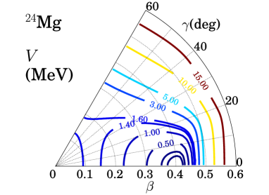
Figure 1: (Color online) Collective potential $V(\beta,\gamma)$ for ²⁴Mg.

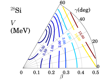
Figure 2: (Color online) Collective potential $V(\beta,\gamma)$ for ²⁸Si.

Figure 3: Neutron Nilsson diagrams calculated within $p$ and $sd$-shell model space as functions of $\beta$ (a) and $\gamma$ (b). Even and odd parity orbits are drawn with solid and dashed lines, respectively.

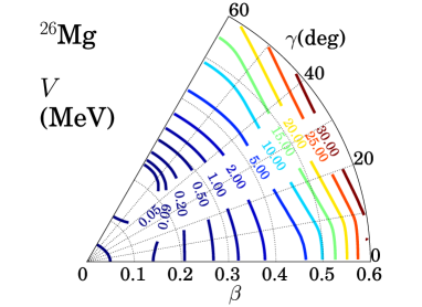
Figure 4: (Color online) Collective potential $V(\beta,\gamma)$ for ²⁶Mg.

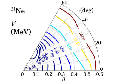
Figure 5: (Color online) Collective potential $V(\beta,\gamma)$ for ²⁴Ne.

In Fig. 6, proton and neutron monopole pairing gaps are plotted as functions of $(\beta,\gamma)$. Basic characters of the proton pairing gaps in ²⁶Mg and ²⁴Ne are same as that in ²⁴Mg, and those of neutron pairing gaps in ²⁶Mg and ²⁴Ne are same as that in ²⁸Si. The proton monopole pairing gaps in ²⁴Mg, ²⁶Mg, and ²⁴Ne show strong ($\beta,\gamma$) dependence; they have the maximum at the spherical point, and they become zero around $\beta\sim 0.4$ in the prolate region. The neutron pairing gaps in ²⁸Si, ²⁶Mg, and ²⁴Ne becomes zero in the oblate region. These zero-gap regions correspond to the prolate $Z=12$ and 10 shell gap and the oblate $N=14$ shell gap in Fig. 3, respectively. Comparing the proton pairing gap for ²⁶Mg with that for ²⁴Mg, and the neutron pairing gap for ²⁶Mg with that for ²⁸Si, an interesting feature is seen in ²⁶Mg; the zero-gap region extends widely in the ($\beta,\gamma$) plane in the case of ²⁶Mg.

In the lower panel of Fig. 3, the neutron Nilsson diagram is shown as functions of $\gamma$ at $\beta=0.3$. The energies of the Nilsson orbits change gradually depending on $\gamma$. Especially, the oblate shell gap at 14 and the prolate shell gap at 12 more smoothly vanish in the $\gamma$ direction than in the $\beta$ direction.

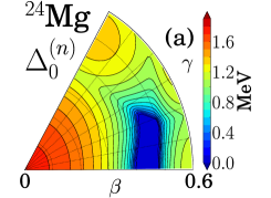
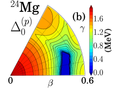
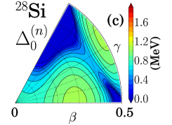
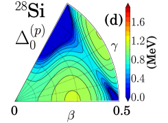
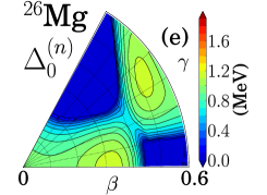
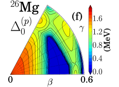
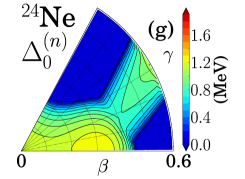
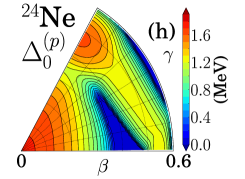
Figure 6: (Color online) Neutron and proton pairing gaps $\Delta_{0}^{(n)}$ and $\Delta_{0}^{(p)}$ for ²⁴Mg, ²⁸Si, ²⁶Mg, and ²⁴Ne.

III.2 Properties of the LQRPA modes

As discussed in the previous subsection, one of the pairing features of the $sd$-shell nuclei is the collapse of the pairing gaps around the deformed shell gaps (Fig. 6). In the former applications of the LQRPA equations to Se and Kr isotopes Hinohara et al. (2010); Sato and Hinohara (2011), where the systems are in the superconducting phase in all over the $(\beta,\gamma)$ region considered, the properties and choices of the LQRPA modes in the normal phase has not been analyzed though they are interesting theoretical issues to be clarified. In Fig. 7, the eigen frequencies squared of the LQRPA modes $\omega^{2}(\beta,\gamma)$, the vibrational part of the metric $W(\beta,\gamma)$, and the neutron and proton monopole pairing gaps $\Delta_{0}^{(n)}$ and $\Delta_{0}^{(p)}$ in ²⁴Mg are plotted as functions of $\gamma$ along the $\beta=0.425$ line.

Let us label the chosen two collective modes in Fig. 7 (a) as ‘mode A’ and ‘mode B’. Mode A denotes the collective mode lower in energy at $\gamma=0^{\circ}$, and this mode jumps around $\gamma=12^{\circ},32^{\circ},36^{\circ}$ and $41^{\circ}$. It becomes the second lowest mode at $\gamma=60^{\circ}$. Mode B denotes the collective mode higher in energy at $\gamma=0^{\circ}$, and this mode jumps around $\gamma=8^{\circ}$ and $25^{\circ}$. It becomes the lowest mode at $\gamma=60^{\circ}$.

As seen in Fig. 7 (c), in the region with $0^{\circ}<\gamma<8^{\circ}$, both the neutron and proton pairing gaps vanish. In this region, lowest four eigen modes are close in energy around 1-2 MeV, and they correspond to the neutron and proton pairing vibrational modes at a normal phase (pair addition and pair annihilation). The fifth mode is chosen as a collective mode (mode A). It has the $\gamma$-vibrational character at the axial limit, and this mode is chosen continuously in the small $\gamma$ where the neutron is normal. One important character in the normal system is that the collectivity of the $\beta$ vibration is weakened Bohr and Mottelson (1998a). In the present case, the $\beta$ vibrational mode is found at around 7 MeV. In this energy region, the $\beta$-vibrational collective mode is sometimes embedded in other non-collective modes. However, the figure shows that one can always find such modes using the minimal metric criterion to select the two collective modes.

Around $8^{\circ}<\gamma<12^{\circ}$, the proton becomes superconducting, and the character of the low-lying modes changes to the neutron pair addition and annihilation, proton pairing vibration, and proton pairing rotation (Nambu-Goldstone mode). Note that in Fig. 7 (a), the zero-energy pairing rotational mode is not shown.

In $12^{\circ}<\gamma<25^{\circ}$, neutrons also become superconducting. As the pairing gaps significantly change as functions of deformation in this region, the low-lying vibrational modes have the pairing vibrational characters, and thus they are not chosen to evaluate the quadrupole collective masses. In this region, the vibrational part of the metric increases.

This situation changes in $25^{\circ}<\gamma<41^{\circ}$. The pairing vibration and quadrupole vibration mix in the lowest LQRPA mode, and the pairing-vibrational character of the lowest mode decreases. Therefore, the lowest LQRPA mode is continuously chosen as a collective mode (mode B) to oblate limit. On the other hand, the other collective mode (mode A) changes in several LQRPA modes in this region, because large quadrupole collectivity appears in these LQRPA modes. The quadrupole collectivities of these modes are similar, and the vibrational part of the metric $W$ is continuous around the jump.

Near the oblate region with $41^{\circ}<\gamma<60^{\circ}$, the lowest two modes are chosen as the collective modes, and are decoupled with other LQRPA modes in energy. At the oblate axial limit, the lowest mode (mode B) becomes the $\gamma$ vibration, and the second lowest mode (mode A) corresponds to the $\beta$ vibration.

This analysis shows that the minimal metric criterion for selecting the two collective modes among low-lying LQRPA modes also works for the situation where the pairing gap vanishes.

Figure 7: (a) The LQRPA eigen frequencies $\omega^{2}$, (b) the vibrational part of the metric $W$, and (c) the neutron and proton monopole pairing gaps $\Delta_{0}^{(\tau)}$ in ²⁴Mg plotted as a function of $\gamma$ for a constant value $\beta=0.425$. In (a), the frequencies squared of low-lying LQRPA eigen modes are denoted with the cross symbols, while the two collective modes chosen at each deformation to calculate the vibrational collective masses are denoted by the filled circles. In (b), the vibrational metrics are denoted by the filled circles, while the vibrational metrics calculated with other possible combinations of the LQRPA modes are denoted by the cross symbols.

III.3 Collective levels

In this subsection, we present the excitation spectra, electric transition properties, and collective wave functions that are obtained by solving the collective Schrödinger equation (11) for $I\leq 6$ states.

III.3.1 ²⁴Mg

The excitation spectra for ²⁴Mg are shown in Fig. 8. The calculation yields an yrast rotational band composed of $0_{1}^{+},2_{1}^{+},4_{1}^{+}$, and $6_{1}^{+}$ states, and an excited side band composed of $2_{2}^{+},3_{1}^{+},4_{2}^{+},5_{1}^{+}$, and $6_{2}^{+}$ states. These two bands are in a very good agreement with the experimental energy levels. To analyze the structure of each state, the vibrational wave functions squared are displayed in Fig. 9, where the $\beta^{4}$ factor is multiplied, which carries the main $\beta$ dependence from the volume element $|G(\beta,\gamma)|^{1/2}d\beta d\gamma$ in Eq. (16). The members of the yrast band are localized around the prolate minimum, showing the prolate character of the yrast rotational band. The vibrational wave functions of the excited band are concentrated in the triaxial region around the prolate minimum with $\gamma\sim 20^{\circ}$. This can be interpreted as the $\gamma$ vibrational band of the prolate yrast state. We also analyze the $K$-component fraction for these states in Table 2. The table shows that the $K$-mixing in these states are very small, and the results support the $K=0$ ground band and $K=2$ excited band. These features are almost unchanged even with the increase of angular momentum.

In Tables 3 and 4, the electric properties of the low-lying states are summarized. In addition to the theoretical results calculated with the effective charges ($e_{\rm eff}^{(n)},e_{\rm eff}^{(p)}$)=(0.5,1.5), we also list the values for pure neutron and proton contributions obtained by using ($e_{\rm eff}^{(n)},e_{\rm eff}^{(p)}$)=(1,0) and (0,1). The calculated results reasonably reproduce the trend of the $E2$ transition strengths though they tend to underestimate the absolute values of experimental data. Using a different set of effective charges improves the systematical underestimation of the theoretical values. However, still there are some disagreement, for example, in $4_{1}^{+}\rightarrow 2_{1}^{+}$, $3_{1}^{+}\rightarrow 2_{2}^{+}$ and $5_{1}^{+}\rightarrow 3_{1}^{+}$ transitions. One can see that the neutron and proton matrix elements are almost equal for all the transitions listed in the table. The prolate feature is shown also in the spectroscopic quadrupole moments. The calculated values for the yrast and the side bands are well described with the estimated values from the rotational collective model of a prolate deformation with $K=0$ and $2$, respectively. This shows the rigid deformation feature in ²⁴Mg.

As mentioned in Introduction, several triaxial GCM calculations are performed for the study of low-lying states in ²⁴Mg employing modern density functionals Yao et al. (2010); Bender and Heenen (2008); Rodríguez and Egido (2010). In comparison with them, the present calculation gives a remarkable agreement with the experimental data for the ground $K=0$ band and the excited $K=2$ band despite the schematic effective interaction and restricted model space. Especially, the agreement in the excitation energies are better than the GCM calculations, while that in the $B(E2)$ values are worse. The small $K$-mixing properties in the ground and excited bands shown in Table 2 are consistent with them Yao et al. (2010); Rodríguez and Egido (2010).

Figure 8: Excitation spectra calculated for ²⁴Mg by means of the CHB+LQRPA method and experimental data ENS .

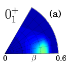
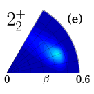
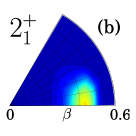
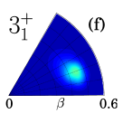
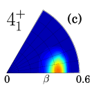
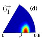
Figure 9: (Color online) Vibrational wave functions squared $\beta^{4}|\Phi_{\alpha I}(\beta,\gamma)|^{2}$ calculated for ²⁴Mg.

Table 2: Probability amplitude of quantum states of ²⁴Mg for each $K$-component.

$I^{\pi}_{\alpha}$	$K=0$	$K=2$	$K=4$	$K=6$
$0_{1}^{+}$	1.00	-	-	-
$2_{1}^{+}$	0.99	0.01	-	-
$4_{1}^{+}$	1.00	0.00	0.00	-
$6_{1}^{+}$	1.00	0.00	0.00	0.00
$2_{2}^{+}$	0.03	0.97	-	-
$3_{1}^{+}$	-	1.00	-	-
$4_{2}^{+}$	0.03	0.95	0.02	-
$5_{1}^{+}$	-	1.00	0.00	-
$6_{2}^{+}$	0.02	0.97	0.01	0.00

Table 3: The values of $B(E2)$ for ²⁴Mg listed in units of $e^{2}$fm⁴. The theoretical values are calculated with the effective charges ($e_{\rm eff}^{(n)},e_{\rm eff}^{(p)}$) = (0.5,1.5). The values calculated from pure neutron contribution ($e_{\rm eff}^{(n)},e_{\rm eff}^{(p)}$) = (1,0) and proton contribution ($e_{\rm eff}^{(n)},e_{\rm eff}^{(p)}$) = (0,1) are also listed. Experimental data are taken from Ref. ENS .

	EXP	CHB+LQRPA	neutron	proton
$2_{1}^{+}\rightarrow 0_{1}^{+}$	88	63.026	16.189	15.614
$4_{1}^{+}\rightarrow 2_{1}^{+}$	160	96.171	24.663	23.838
$6_{1}^{+}\rightarrow 4_{1}^{+}$	155	108.032	27.684	26.784
$3_{1}^{+}\rightarrow 2_{2}^{+}$	239	103.484	26.686	25.602
$4_{2}^{+}\rightarrow 3_{1}^{+}$	-	80.216	20.674	19.849
$5_{1}^{+}\rightarrow 4_{2}^{+}$	-	57.085	14.713	14.125
$6_{2}^{+}\rightarrow 5_{1}^{+}$	-	47.575	12.220	11.786
$4_{2}^{+}\rightarrow 2_{2}^{+}$	64	44.673	11.448	11.076
$5_{1}^{+}\rightarrow 3_{1}^{+}$	149	65.981	16.944	16.347
$6_{2}^{+}\rightarrow 4_{2}^{+}$	-	83.500	21.415	20.697
$4_{1}^{+}\rightarrow 2_{2}^{+}$	-	0.011	0.003	0.003
$2_{2}^{+}\rightarrow 2_{1}^{+}$	15	17.197	4.216	4.327
$2_{2}^{+}\rightarrow 0_{1}^{+}$	8	4.911	1.179	1.244
$3_{1}^{+}\rightarrow 4_{1}^{+}$	-	5.091	1.241	1.284
$3_{1}^{+}\rightarrow 2_{1}^{+}$	10	8.180	1.948	2.078
$4_{2}^{+}\rightarrow 4_{1}^{+}$	-	12.100	2.925	3.059
$6_{1}^{+}\rightarrow 4_{2}^{+}$	-	0.018	0.004	0.005
$4_{2}^{+}\rightarrow 2_{1}^{+}$	5	3.493	0.849	0.882
$5_{1}^{+}\rightarrow 6_{1}^{+}$	-	4.217	1.018	1.066
$5_{1}^{+}\rightarrow 4_{1}^{+}$	-	7.618	1.825	1.931
$6_{2}^{+}\rightarrow 6_{1}^{+}$	-	9.756	2.348	2.470
$6_{2}^{+}\rightarrow 4_{1}^{+}$	-	3.534	0.867	0.889

Table 4: Spectroscopic quadrupole moments for ²⁴Mg listed in units of $e$ fm². See also caption in Table 3. Experimental data are taken from Ref. ENS .

	EXP	CHB+LQPRA	neutron	proton
$Q(2_{1}^{+})$	$-$16.6	$-$15.7	$-$7.97	$-$7.81
$Q(4_{1}^{+})$	-	$-$20.8	$-$10.5	$-$10.4
$Q(6_{1}^{+})$	-	$-$23.7	$-$12.0	$-$11.8
$Q(2_{2}^{+})$	-	15.5	7.87	7.72
$Q(3_{1}^{+})$	-	0	0	0
$Q(4_{2}^{+})$	-	$-$5.85	$-$3.00	$-$2.90
$Q(5_{1}^{+})$	-	$-$13.0	$-$6.58	$-$6.45
$Q(6_{2}^{+})$	-	$-$14.4	$-$7.34	$-$7.16

III.3.2 ²⁸Si

In addition to the ground rotational band, we show two rotational bands built on the $2_{2}^{+}$ and $0_{2}^{+}$ states in Fig. 10. The values of $B(E2)$ and spectroscopic quadrupole moments are summarized in Tables 5 and 6, and the vibrational wave functions squared in $(\beta,\gamma)$ plane are shown in Fig. 11. The vibrational wave functions and the quadrupole moments indicate the oblate deformation of the yrast rotational band. In Table 7, the $K$ mixing in each state is listed. The yrast rotational band is consistent with $K=0$ oblate band. It is seen that the spectroscopic quadrupole moment significantly increases with the increase of the angular momentum. The values of $Q(4_{1}^{+})$ and $Q(6_{1}^{+})$ are larger than those estimated from the rotational collective model using the calculated $Q(2_{1}^{+})$ value. (In the case of the $6_{1}^{+}$ state, 16.8 $e$ fm² is the estimated value for $K=0$ rotational band.) This indicates that the $\beta$ deformation of the intrinsic state grows as the angular momentum increases in the yrast band as seen in Fig. 11.

We then compare the theoretical results for the ground band with the experimental data. The theoretical results overestimate both of the excitation energies and $B(E2)$ values for $4_{1}^{+}$ and $6_{1}^{+}$ states. The experimental values of $B(E2)$ do not follow the trend of the collective model. This indicates that the spin alignment of the single-particle states plays a role in the high angular momentum states, and this reduces the $B(E2)$ values. In the quadrupole collective Hamiltonian which we derive in the present calculation, the moments of inertia are evaluated at zero angular momentum, and the alignment of the single-particle states is not taken into account. To include such effect by using the cranked mean field approach is an interesting extension of the model, but is beyond the scope of this paper.

The vibrational wave functions of the theoretical $0_{2}^{+}$, $2_{3}^{+}$, and $4_{3}^{+}$ states have nodes in the $\beta$ direction, and this can be interpreted as the $\beta$-vibrational behavior on top of the oblate yrast states. The fact that in-band transitions in the $\beta$-vibrational band $B(E2;2_{3}^{+}\rightarrow 0_{2}^{+})$ is comparable with those of the ground rotational band $B(E2;2_{1}^{+}\rightarrow 0_{1}^{+})$, and the positive sign of the quadrupole moment in $2_{3}^{+}$ and $4_{3}^{+}$ supports this interpretation. However, they contain $K$ mixing and shape mixing with the prolate region in the vibrational wave functions.

The excited band composed of $2_{2}^{+}$, $3_{1}^{+}$, $4_{2}^{+}$, $5_{1}^{+}$, and $6_{2}^{+}$ states are also found in the calculation. The main component of the vibrational wave functions is $K=2$, and lies in the triaxially deformed region. However, there is no experimental information corresponding to this triaxial band. Since the prolate local minimum is not found in the collective potential, the prolate rotational band does not obtained in the energy spectrum.

Figure 10: Excitation spectra calculated for ²⁸Si by means of the CHB+LQRPA method and experimental data ENS .

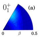
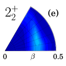
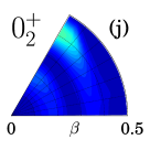
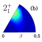
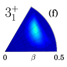
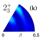
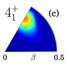
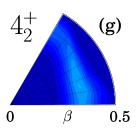
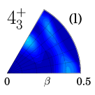
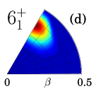
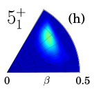
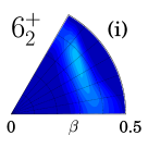
Figure 11: (Color online) Vibrational wave functions squared $\beta^{4}|\Phi_{\alpha I}(\beta,\gamma)|^{2}$ calculated for ²⁸Si.

Table 5: The values of $B(E2)$ for ²⁸Si listed in units of $e^{2}$fm⁴. See also caption in Table 3. Experimental data are taken from Ref. ENS .

	EXP	CHB+LQRPA	neutron	proton
$2_{1}^{+}\rightarrow 0_{1}^{+}$	66.7	41.558	10.497	10.354
$4_{1}^{+}\rightarrow 2_{1}^{+}$	69.7	77.816	19.635	19.394
$6_{1}^{+}\rightarrow 4_{1}^{+}$	50.0	98.715	24.893	24.608
$3_{1}^{+}\rightarrow 2_{2}^{+}$	-	65.783	16.517	16.422
$4_{2}^{+}\rightarrow 3_{1}^{+}$	-	41.612	10.515	10.366
$5_{1}^{+}\rightarrow 4_{2}^{+}$	-	27.185	6.840	6.782
$6_{2}^{+}\rightarrow 5_{1}^{+}$	-	30.972	7.815	7.719
$4_{2}^{+}\rightarrow 2_{2}^{+}$	-	59.403	14.918	14.828
$5_{1}^{+}\rightarrow 3_{1}^{+}$	-	62.666	15.768	15.633
$6_{2}^{+}\rightarrow 4_{2}^{+}$	-	98.322	24.709	24.538
$2_{3}^{+}\rightarrow 0_{2}^{+}$	27.8	44.347	11.187	11.053
$4_{3}^{+}\rightarrow 2_{3}^{+}$	-	55.761	14.108	13.884
$4_{1}^{+}\rightarrow 2_{2}^{+}$	-	0.450	0.118	0.111
$2_{2}^{+}\rightarrow 2_{1}^{+}$	-	30.834	7.592	7.748
$2_{2}^{+}\rightarrow 0_{1}^{+}$	-	2.618	0.617	0.667
$3_{1}^{+}\rightarrow 4_{1}^{+}$	-	8.124	1.970	2.051
$3_{1}^{+}\rightarrow 2_{1}^{+}$	-	5.910	1.387	1.508
$4_{2}^{+}\rightarrow 4_{1}^{+}$	-	19.928	4.864	5.022
$6_{1}^{+}\rightarrow 4_{2}^{+}$	-	0.432	0.115	0.106
$4_{2}^{+}\rightarrow 2_{1}^{+}$	-	2.135	0.508	0.542
$5_{1}^{+}\rightarrow 6_{1}^{+}$	-	5.897	1.408	1.497
$5_{1}^{+}\rightarrow 4_{1}^{+}$	-	6.951	1.638	1.772
$6_{2}^{+}\rightarrow 6_{1}^{+}$	-	15.752	3.813	3.980
$6_{2}^{+}\rightarrow 4_{1}^{+}$	-	2.836	0.683	0.718
$0_{2}^{+}\rightarrow 2_{1}^{+}$	-	56.831	14.217	14.205
$2_{3}^{+}\rightarrow 0_{1}^{+}$	-	0.078	0.021	0.019
$2_{3}^{+}\rightarrow 2_{1}^{+}$	-	2.571	0.623	0.649
$2_{3}^{+}\rightarrow 4_{1}^{+}$	-	16.159	4.033	4.042

Table 6: Spectroscopic quadrupole moments for ²⁸Si listed in units of $e$ fm². See also captions in Table 3. Experimental data are taken from Ref. ENS .

	EXP	CHB+LQRPA	neutron	proton
$Q(2_{1}^{+})$	16	12.0	6.05	5.98
$Q(4_{1}^{+})$	-	17.8	8.99	8.90
$Q(6_{1}^{+})$	-	22.2	11.2	11.1
$Q(2_{2}^{+})$	-	$-$12.6	$-$6.33	$-$6.29
$Q(3_{1}^{+})$	-	0	0	0
$Q(4_{2}^{+})$	-	$-$3.10	$-$1.55	$-$1.55
$Q(5_{1}^{+})$	-	10.3	5.16	5.12
$Q(6_{2}^{+})$	-	1.61	0.83	0.80
$Q(2_{3}^{+})$	-	9.69	4.89	4.83
$Q(4_{3}^{+})$	-	7.35	3.69	3.67

Table 7: Probability amplitude of quantum states of ²⁸Si for each $K_{2}$-component, where $K_{2}$ is the projection of the angular momentum onto the symmetric axis at $\gamma=60^{\circ}$.

$I^{\pi}_{\alpha}$	$K_{2}=0$	$K_{2}=2$	$K_{2}=4$	$K_{2}=6$
$0_{1}^{+}$	1.00	-	-	-
$2_{1}^{+}$	0.97	0.03	-	-
$4_{1}^{+}$	0.98	0.02	0.00	-
$6_{1}^{+}$	0.99	0.01	0.00	0.00
$2_{2}^{+}$	0.11	0.89	-	-
$3_{1}^{+}$	-	1.00	-	-
$4_{2}^{+}$	0.16	0.71	0.14	-
$5_{1}^{+}$	-	0.97	0.03	-
$6_{2}^{+}$	0.15	0.71	0.09	0.04
$0_{2}^{+}$	1.00	-	-	-
$2_{3}^{+}$	0.94	0.06	-	-
$4_{3}^{+}$	0.67	0.20	0.14	-

III.3.3 ²⁶Mg

By adding two neutrons to the prolately deformed ²⁴Mg, the character of collective dynamics in the low-lying levels drastically changes from that of ²⁴Mg. Figure 12 compares the theoretical and experimental low-lying energy levels in ²⁶Mg. In addition to the yrast band ($0_{1}^{+},2_{1}^{+},4_{1}^{+}$ and $6_{1}^{+}$), we show a side band composed of $2_{2}^{+},3_{1}^{+},4_{2}^{+},5_{1}^{+}$, and $6_{2}^{+}$ states, which are connected by relatively large $B(E2)$ values (see Table 8).

The vibrational wave functions squared are shown in Fig. 13. A significant difference from ²⁴Mg is seen in the deformation property of the vibrational wave functions of the ground $0_{1}^{+}$ state. In contrast to the well-developed prolate structure of the ²⁴Mg yrast band, the $0_{1}^{+}$ state of ²⁶Mg spreads over the triaxial region from oblate to prolate ones, although the shallow potential minimum is located at the oblate region. This indicates the very $\gamma$-soft character of the ground state. The members of the yrast band tend to localize around the prolate shape as the angular momentum increases. As for the excitation energies of the yrast band, the $E_{x}(4^{+}_{1})/E_{x}(2^{+}_{1})$ ratio is 2.64 in theoretical calculation, which explains the experimental value 2.71 very well. As seen in Table 9, the spectroscopic quadrupole moments of the yrast band are consistent with the prolate deformation, but the absolute values are relatively smaller than those of ²⁴Mg. Moreover, $Q(6_{1}^{+})$ is almost twice of $Q(2_{1}^{+})$, and this is much larger than the value of $K=0$ rotational collective model, indicating that the development of the prolate deformation with increase of the angular momentum. This feature is also seen in the ratio $B(E2;4_{1}^{+}\rightarrow 2_{1}^{+})/B(E2;2_{1}^{+}\rightarrow 0_{1}^{+})$. The theoretical value of the ratio is 1.7, which is larger than the collective model value 1.43. However, the experimental value of the ratio 1.05 again indicates the effect of the single-particle alignment.

The quantum states in the side band distribute widely in the $\gamma$ direction. This character is remarkably different from that of ²⁴Mg, where all the members of the $K=2$ side band are localized in the triaxial region close to the prolate local minimum (Fig. 9). In particular, an oblate character develops in even angular momentum states of the side band, and the $4_{2}^{+}$ and $6_{2}^{+}$ states form the two-peak structure in the oblate and prolate region. This two-peak structure indicates the $\gamma$-soft character of the collective potential as discussed in Ref. Sato et al. (2010).

Figure 12: Excitation spectra calculated for ²⁶Mg by means of the CHB+LQRPA method and experimental data ENS .

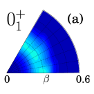
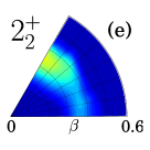
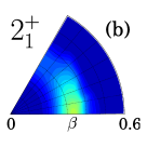
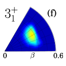
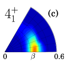
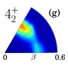
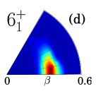
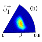
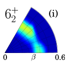
Figure 13: (Color online) Vibrational wave functions squared $\beta^{4}|\Phi_{\alpha I}(\beta,\gamma)|^{2}$ calculated for ²⁶Mg.

Table 8: The values of $B(E2)$ for ²⁶Mg listed in units of $e^{2}$fm⁴. See also caption in Table 3. Experimental values are taken from Refs. ENS ; Glatz et al. (1986), and the assignment of the levels are given in Ref. Glatz et al. (1986).

	EXP	CHB+LQRPA	neutron	proton
$2_{1}^{+}\rightarrow 0_{1}^{+}$	61.3	52.870	11.131	13.953
$4_{1}^{+}\rightarrow 2_{1}^{+}$	64.1	90.302	18.379	24.070
$6_{1}^{+}\rightarrow 4_{1}^{+}$	-	112.596	23.016	29.975
$3_{1}^{+}\rightarrow 2_{2}^{+}$	41.2	74.890	13.707	20.568
$4_{2}^{+}\rightarrow 3_{1}^{+}$	37.0	20.437	1.366	6.887
$5_{1}^{+}\rightarrow 4_{2}^{+}$	-	32.073	4.387	9.470
$6_{2}^{+}\rightarrow 5_{1}^{+}$	-	19.052	1.654	6.156
$4_{2}^{+}\rightarrow 2_{2}^{+}$	23.8a	58.789	16.303	14.180
$5_{1}^{+}\rightarrow 3_{1}^{+}$	-	70.150	14.724	18.530
$6_{2}^{+}\rightarrow 4_{2}^{+}$	-	88.693	23.078	21.876
$4_{1}^{+}\rightarrow 2_{2}^{+}$	16.0a	2.073	0.131	0.704
$2_{2}^{+}\rightarrow 2_{1}^{+}$	28.4	62.940	19.792	14.486
$2_{2}^{+}\rightarrow 0_{1}^{+}$	1.60	0.765	2.040	0.011
$3_{1}^{+}\rightarrow 4_{1}^{+}$	-	18.259	5.971	4.138
$3_{1}^{+}\rightarrow 2_{1}^{+}$	0.23a	0.456	3.234	0.022
$4_{2}^{+}\rightarrow 4_{1}^{+}$	-	28.948	12.298	5.847
$6_{1}^{+}\rightarrow 4_{2}^{+}$	-	0.635	0.022	0.232
$4_{2}^{+}\rightarrow 2_{1}^{+}$	-	1.536	1.755	0.148
$6_{1}^{+}\rightarrow 5_{1}^{+}$	-	13.227	4.769	2.879
$5_{1}^{+}\rightarrow 4_{1}^{+}$	-	0.773	2.999	0.000
$6_{2}^{+}\rightarrow 6_{1}^{+}$	-	18.167	9.774	3.238
$6_{2}^{+}\rightarrow 4_{1}^{+}$	-	1.113	1.006	0.136

Table 9: Spectroscopic quadrupole moment for ²⁶Mg listed in units of $e$ fm². See also caption in Table 3. Experimental data are taken from Ref. ENS .

	EXP	CHB+LQRPA	neutron	proton
$Q(2_{1}^{+})$	$-$13.5	$-$9.07	$-$2.33	$-$5.27
$Q(4_{1}^{+})$	-	$-$14.9	$-$4.44	$-$8.48
$Q(6_{1}^{+})$	-	$-$17.9	$-$5.61	$-$10.1
$Q(2_{2}^{+})$	-	7.17	2.51	3.95
$Q(3_{1}^{+})$	-	0	0	0
$Q(4_{2}^{+})$	-	2.74	2.84	0.88
$Q(5_{1}^{+})$	-	$-$7.96	$-$1.91	$-$4.67
$Q(6_{2}^{+})$	-	$-$3.25	1.60	$-$2.70

III.3.4 ²⁴Ne

Figures 14 and 15 display the energy spectra and vibrational wave functions squared for ²⁴Ne, and the $B(E2)$ and the spectroscopic quadrupole moments are listed in Tables 10 and 11. The theoretical yrast band $0_{1}^{+}$, $2_{1}^{+}$, $4_{1}^{+}$, and $6_{1}^{+}$ has the $\gamma$-soft character similar to that of ²⁶Mg; the vibrational wave function of the $0_{1}^{+}$ state has a peak at the oblate region, but spreads over the triaxial region. Moreover, the gradual shape change in the yrast states with the increase of angular momentum is also found in the calculation. The oblate peak of the vibrational wave function in the $0_{1}^{+}$ state shifts to the prolate region in the $4_{1}^{+}$ state.

The spectroscopic quadrupole moments of the yrast band are consistent with the prolate deformation, but the absolute values are smaller than ²⁶Mg.

The two-peak structure in the $2_{2}^{+},4_{2}^{+}$, and $6_{2}^{+}$ states in the side band is also seen in ²⁴Ne showing again the $\gamma$-soft character as well as ²⁶Mg.

The excitation energy of the $2_{1}^{+}$ state and $B(E2;2_{1}^{+}\rightarrow 0_{1}^{+})$ are reproduced by the theoretical calculation. However, the experimental energy spectrum is much more vibrational than the theoretical one.

Figure 14: Excitation spectra calculated for ²⁴Ne by means of the CHB+LQRPA method and experimental data  ENS .

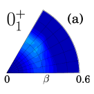
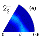
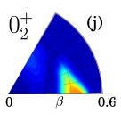
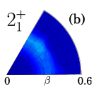
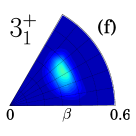
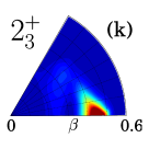
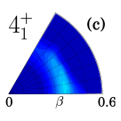
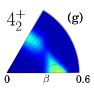
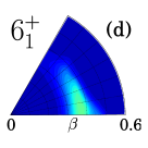
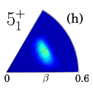
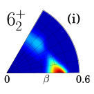
Figure 15: (Color online) Vibrational wave functions squared $\beta^{4}|\Phi_{\alpha I}(\beta,\gamma)|^{2}$ calculated for ²⁴Ne.

Table 10: The values of $B(E2)$ for ²⁴Ne listed in units of $e^{2}$fm⁴. See also caption in Table 3. Experimental data are taken from Ref. ENS

	EXP	CHB+LQRPA	neutron	proton
$2_{1}^{+}\rightarrow 0_{1}^{+}$	28.0	33.576	14.124	6.813
$4_{1}^{+}\rightarrow 2_{1}^{+}$	-	56.446	21.854	11.906
$6_{1}^{+}\rightarrow 4_{1}^{+}$	-	74.510	27.395	16.080
$3_{1}^{+}\rightarrow 2_{2}^{+}$	-	45.159	17.889	9.426
$4_{2}^{+}\rightarrow 3_{1}^{+}$	-	6.841	0.171	2.579
$5_{1}^{+}\rightarrow 4_{2}^{+}$	-	15.843	4.637	3.747
$6_{2}^{+}\rightarrow 5_{1}^{+}$	-	7.551	0.550	2.512
$4_{2}^{+}\rightarrow 2_{2}^{+}$	-	39.297	15.416	8.239
$5_{1}^{+}\rightarrow 3_{1}^{+}$	-	44.036	16.045	9.540
$6_{2}^{+}\rightarrow 4_{2}^{+}$	-	61.481	23.999	12.919
$2_{3}^{+}\rightarrow 0_{2}^{+}$	-	29.908	12.458	6.098
$4_{1}^{+}\rightarrow 2_{2}^{+}$	-	3.298	0.419	0.990
$2_{2}^{+}\rightarrow 2_{1}^{+}$	-	53.242	22.961	10.675
$2_{2}^{+}\rightarrow 0_{1}^{+}$	-	0.361	0.861	0.504
$3_{1}^{+}\rightarrow 4_{1}^{+}$	-	20.227	9.280	3.932
$4_{1}^{+}\rightarrow 3_{1}^{+}$	-	15.732	7.218	3.058
$3_{1}^{+}\rightarrow 2_{1}^{+}$	-	1.487	1.542	1.505
$4_{2}^{+}\rightarrow 4_{1}^{+}$	-	23.575	14.274	3.911
$6_{1}^{+}\rightarrow 4_{2}^{+}$	-	2.375	0.325	0.701
$4_{2}^{+}\rightarrow 2_{1}^{+}$	-	0.116	1.450	0.030
$5_{1}^{+}\rightarrow 6_{1}^{+}$	-	16.505	8.537	3.008
$5_{1}^{+}\rightarrow 4_{1}^{+}$	-	0.642	2.095	1.034
$6_{2}^{+}\rightarrow 6_{1}^{+}$	-	13.261	11.282	1.711
$6_{2}^{+}\rightarrow 4_{1}^{+}$	-	0.115	0.785	0.005
$2_{2}^{+}\rightarrow 0_{2}^{+}$	-	16.025	4.635	3.807
$0_{2}^{+}\rightarrow 2_{2}^{+}$	-	80.124	23.175	19.034
$0_{2}^{+}\rightarrow 2_{1}^{+}$	-	23.593	5.891	5.901
$2_{3}^{+}\rightarrow 0_{1}^{+}$	-	0.464	0.044	0.274
$2_{3}^{+}\rightarrow 2_{1}^{+}$	-	1.843	0.567	0.428
$2_{3}^{+}\rightarrow 4_{1}^{+}$	-	6.076	2.253	1.306

Table 11: Spectroscopic quadrupole moments for ²⁴Ne listed in units of $e$ fm². See also caption in Table 3.

	EXP	CHB+LQRPA	neutron	proton
$Q(2_{1}^{+})$	-	$-$2.71	1.28	$-$2.23
$Q(4_{1}^{+})$	-	$-$8.10	$-$0.22	$-$5.33
$Q(6_{1}^{+})$	-	$-$11.6	$-$1.44	$-$7.24
$Q(2_{2}^{+})$	-	$-$0.21	$-$1.68	0.42
$Q(3_{1}^{+})$	-	0	0	0
$Q(4_{2}^{+})$	-	$-$4.68	$-$1.75	$-$2.54
$Q(5_{1}^{+})$	-	$-$5.16	$-$0.47	$-$3.28
$Q(6_{2}^{+})$	-	$-$9.38	$-$2.80	$-$5.32
$Q(2_{3}^{+})$	-	$-$8.16	$-$4.94	$-$3.79

IV Discussion

IV.1 Rotational hindrance of shape mixing in ²⁶Mg and ²⁴Ne

Here, we discuss the character of the vibrational wave functions in more detail. What is commonly seen in the calculated results for ²⁶Mg and ²⁴Ne is the localization of the vibrational wave functions squared as the increase of the angular momentum. While the ground $0_{1}^{+}$ state spreads over the $\gamma$ direction, the yrast band tends to localize in the ($\beta,\gamma$) plane around the prolate region, even though the collective potential has the shallow oblate minimum.

This rotational hindrance of shape mixing is also seen in the cases of oblate-prolate shape coexistence Hinohara et al. (2009); Sato et al. (2010) and can be understood from the deformation dependence of the rotational moments of inertia. Figure 16 shows the rotational moments of inertia about the intermediate axis, ${\cal J}_{1}(\beta,\gamma)$, for ^24,26Mg, ²⁴Ne, and ²⁸Si. An oblate-prolate asymmetry is seen in the rotational moments of inertia; ${\cal J}_{1}(\beta,\gamma)$ for ²⁶Mg and ²⁴Ne becomes larger in the prolate side than the oblate side for the constant $\beta$ value. This is the reason why the prolate shape is favored especially for high angular momentum states. Moreover, due to the strong shell effect there exists a maximum point of the rotational moment of inertia in the $(\beta,\gamma)$ plane, which is inconsistent with the ideal irrotational moments of inertia proportional to the $\beta^{2}$. As is well known, the pairing correlation decreases the moment of inertia Ring and Schuck (1980), and in the region where the pairing gap vanishes, the moment of inertia becomes larger. In the case of ²⁶Mg, the neutron and proton pairing gaps vanish in the prolate region where the moment of inertia becomes large in this region (Fig. 6). Because of the behavior of the rotational moments of inertia, this prolate region is favored in rotational kinetic energy, while it is unfavored in collective potential energy, which increases as the deformation increases. As a result, the vibrational wave function for higher angular momentum states localizes, and the $\beta$- or $\gamma$-soft nature of the vibrational wave function is hindered.

The change of the yrast state structure discussed above is also seen in ²⁸Si. In the case of ²⁸Si, one can see that the deformation of the vibrational wave function grows as angular momentum increases. The minimum of the collective potential locates around $\beta=0.26$, while the maximum of the moment of inertia locates around $\beta=0.36$ in the oblate side. This is the reason why the deformation increases in the yrast band of ²⁸Si. In case of ²⁴Mg, however, the minimum of the collective potential and the maximum of the moment of inertia coincide around $\beta=0.41$, and such a change in the structure of the yrast band does not occur.

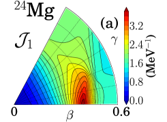
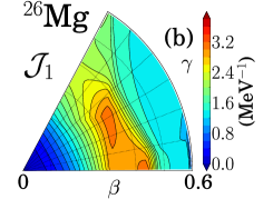
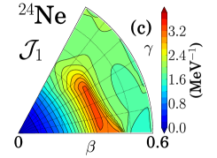
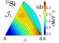
Figure 16: (Color online) Rotational moments of inertia about the intermediate axis, ${\cal J}_{1}(\beta,\gamma)$.

IV.2 Analysis with mirror nucleus method

One of the interesting issues in $N\neq Z$ nuclei in the middle of $sd$-shell region is the properties of the neutron and proton quadrupole transition matrix elements. In the mirror nucleus method Bernstein et al. (1979), the proton matrix element $M_{p}$ is determined from the $E2$ transitions as $B(E2;I\rightarrow I^{\prime})=M^{2}_{p}/(2I+1)$, while the neutron one $M_{n}$ is determined from the same $E2$ transitions of the mirror nucleus as $B_{\rm mirror}(E2;I\rightarrow I^{\prime})=M^{2}_{n}/(2I+1)$. Although the $M_{n}/M_{p}$ ratio should be equal to the ratio $N/Z$ in the simple collective model, it has been experimentally suggested that the $M_{n}/M_{p}$ ratio for the ground band transitions deviates from $N/Z$ in some $N\neq Z$ nuclei Bernstein et al. (1981); Kanno et al. (2002) indicating possible difference between proton and neutron shapes or shape dynamics. Moreover, the $M_{n}/M_{p}$ ratio for the $2^{+}_{2}\rightarrow 0^{+}_{1}$ transition in ²⁶Mg is known to be extremely larger than the expected value $N/Z$ in mirror nucleus method and also in the analysis of $(p,p^{\prime})$ scattering reactions Alons et al. (1981); Sciuccati et al. (1985). The value of $(M_{n}/M_{p})/(N/Z)$ is $1.83\pm 0.34$ ENS . This clearly indicates the dominance of the neutron matrix element in this transition. In this subsection, we discuss the origin of the neutron dominance in the $2_{2}^{+}\rightarrow 0_{1}^{+}$ transition in ²⁶Mg in terms of the large-amplitude triaxial shape dynamics. We also discuss the yrast transition $2_{1}^{+}\rightarrow 0_{1}^{+}$ in ²⁶Mg and ²⁴Ne.

IV.2.1 $2_{2}^{+}\rightarrow 0_{1}^{+}$ transition in ²⁶Mg

In Table 12, the experimental and theoretical values for $B(E2;2_{2}^{+}\rightarrow 0_{1}^{+})$ transition are summarized. The theoretical value $(M_{n}/M_{p})/(N/Z)=2.15$ reproduces the neutron dominance very well. Actually, the bare proton contribution to this transition in ²⁶Mg is more than hundred times smaller than the neutron one. As seen from Table 3 and 5, such difference cannot be found in $N=Z$ nuclei. The shell model value 2.10 Brown et al. (1982) given with the effective charges $(e_{n},e_{p})=(0.35,1.35)$ also explains the neutron dominance of this transition.

To analyze the mechanism of the neutron dominance in this transition, we present the $E2$ transition density $\rho_{\alpha I\alpha^{\prime}I^{\prime}}^{(E2)}(\beta,\gamma)$ defined in Eq. (22) for ²⁶Mg in Fig. 17. Let us first compare $E2$ transition densities for $2_{1}^{+}\rightarrow 0_{1}^{+}$ and $2_{2}^{+}\rightarrow 0_{1}^{+}$. Because of the structure of the yrast vibrational wave functions, the sign of the transition density for the former in-band transition is positive all over the $(\beta,\gamma)$ deformation, while the transition density for the latter transition changes its sign in the $(\beta,\gamma)$ plane, since the vibrational wave function of an excited state has nodes in the $(\beta,\gamma)$ plane. In the case of the $2_{2}^{+}\rightarrow 0_{1}^{+}$ transition as seen in Fig. 17, the sign of the transition density is opposite in the prolate region and oblate region, and this results in the cancellation after the $(\beta,\gamma)$ integration. In the case of ²⁶Mg, the proton matrix element is almost completely canceled after the integration of the transition density. Concerning the neutrons, the contribution to this transition density is relatively larger in the oblate region than in the prolate region, since the neutron favors the oblate deformation for $N=14$ system. This situation produces the large $M_{n}/M_{p}$ ratio.

This cancellation taking place in the $(\beta,\gamma)$ plane is the result of the large-amplitude collective dynamics in the $(\beta,\gamma)$ plane, especially in the $\gamma$ direction. The importance of triaxial degree of freedom is clearly seen from Fig. 18, where the $E2$ transition density is plotted as a function of $\gamma$ for a constant value of $\beta$. It is seen that the proton transition density is almost anti-symmetric with respect to $\gamma=30^{\circ}$, while the asymmetry is present for neutron transition density.

Table 12: The values of $B(E2;2_{2}^{+}\rightarrow 0_{1}^{+})$ for ²⁶Mg and ²⁶Si listed in units of $e^{2}$fm⁴. Theoretical values for ²⁶Mg are calculated with the effective charges $(e^{(n)}_{\rm eff},e^{(p)}_{\rm eff})=(0.5,1.5)$, while those for ²⁶Si are calculated assuming the mirror symmetry. The bare neutron and proton contributions calculated with $(e^{(n)}_{\rm eff},e^{(p)}_{\rm eff})=(1,0)$ and (0,1) are also listed. Experimental data and shell model calculation are taken from Refs. ENS , and Brown et al. (1982), respectively.

	EXP	CHB+LQRPA	neutron	proton	SM
26Mg	1.60$\pm$0.32	0.765	2.040	0.011	3.28
26Si	7.32$\pm$2.28	4.82	0.011	2.040	19.7

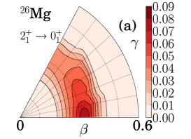
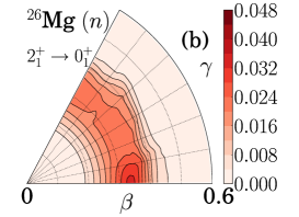
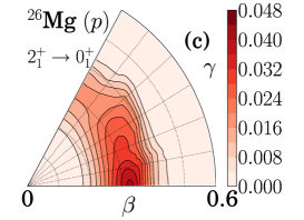
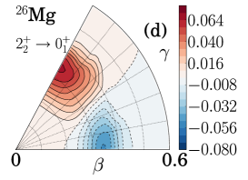
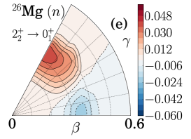
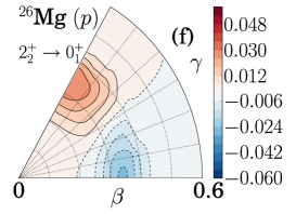
Figure 17: (Color online) $E2$ transition density $\beta^{4}\rho^{(E2)}_{\alpha I\alpha^{\prime}I^{\prime}}(\beta,\gamma)$ for $2_{1}^{+}\rightarrow 0_{1}^{+}$ and $2_{2}^{+}\rightarrow 0_{1}^{+}$ transitions in ²⁶Mg. Three sets of effective charges $(e_{\rm eff}^{(n)},e_{\rm eff}^{(p)})$ =(0.5,1.5), (1,0) and (0,1) are used for left, middle and right panels, respectively.

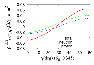
Figure 18: (Color online) $E2$ transition density $\beta^{4}\rho^{E2}_{\alpha I\alpha^{\prime}I^{\prime}}(\beta,\gamma)$ for $2_{2}^{+}\rightarrow 0_{1}^{+}$ transition in ²⁶Mg at $\beta=0.345$ is plotted as function of $\gamma$. The red solid, green dashed, and blue dotted lines show the calculations with three sets of effective charges, $(e^{(n)}_{\rm eff},e^{(p)}_{\rm eff})$= (0.5,1.5), (1,0), and (0,1), respectively.

IV.2.2 $2_{1}^{+}\rightarrow 0_{1}^{+}$ transition in ²⁶Mg and ²⁴Ne

In contrast to the large $(M_{n}/M_{p})/(N/Z)$ for the $2_{2}^{+}\rightarrow 0_{1}^{+}$ transition discussed above, the experimental value of the ratio $(M_{n}/M_{p})/(N/Z)$ for the $2_{1}^{+}\rightarrow 0_{1}^{+}$ transition in ²⁶Mg is $0.92\pm 0.05$, which is close to unity. This indicates that a simple collective model picture with the usual assumption that the radius and the deformation for neutrons are consistent with those for protons is expected to hold. In the case of ²⁴Ne, the experimental value of this ratio is $0.59\pm 0.11$. The possible suppression of the ratio from unity may suggest that the simple picture does not hold for neutrons and protons in this system, and the smaller neutron deformation than the proton deformation is expected in the ground state of ²⁴Ne Kanada-En’yo (2005).

We evaluate the $M_{n}/M_{p}$ ratio by using the mirror nucleus method. In Table 13, $B(E2;2_{1}^{+}\rightarrow 0_{1}^{+})$ values for ²⁶Mg, ²⁶Si, ²⁴Ne, and ²⁴Si are summarized. The relative magnitudes of $E2$ transition probability for mirror pairs cannot be satisfactory reproduced by the theoretical calculation both for $A=24$ and 26 systems.

The theoretical value of the ratio $(M_{n}/M_{p})/(N/Z)$ for ²⁶Mg is 0.81. The calculated value is smaller than unity, and qualitatively reproduces the tendency of the experimental value. The shell model value Brown et al. (1982) gives smaller ratio 0.69 than the present calculation. For ²⁴Ne, the ratio is calculated to be 0.86. The results for ²⁴Ne fail to quantitatively describe the suppression of the ratio extracted from the central values of the experimental $B(E2)$. For more detailed discussions, precise measurements of the $E2$ transition strengths for ²⁴Ne and ²⁴Si are required.

Table 13: The values of $B(E2;2_{1}^{+}\rightarrow 0_{1}^{+})$ for ²⁶Mg, ²⁶Si, ²⁴Ne, and ²⁴Si are summarized in units of $e^{2}$fm⁴. Theoretical values for ²⁶Si and ²⁴Si are calculated assuming the mirror symmetry. See also caption in Table 12. Experimental values and shell model values are taken from Refs. Kanno et al. (2002); Cottle et al. (2001); ENS , and Ref. Brown et al. (1982), respectively.

	EXP	CHB+LQRPA	neutron	proton	SM
26Mg	61.4$\pm$ 1.8	52.870	11.131	13.953	57.1
26Si	70.5$\pm$ 6.9	47.226	13.953	11.131	36.5
24Ne	28.0$\pm$ 6.6	33.576	14.124	6.813	-
24Si	19.1$\pm$ 5.9	48.197	6.813	14.124	-

V Summary

Large-amplitude triaxial quadrupole deformation dynamics in the low-lying states of $sd$-shell nuclei, ²⁴Mg, ²⁸Si, ²⁶Mg, and ²⁴Ne are analyzed on the basis of the quadrupole collective Hamiltonian derived microscopically from the CHFB + LQRPA method.

As for the $N=Z$ systems, the calculation reproduces the prolate rotational band and the $\gamma$ vibrational band in ²⁴Mg, and the oblate rotational band and the $\beta$ vibrational band in ²⁸Si. As for $N\neq Z$ systems, ²⁶Mg and ²⁴Ne, the collective potentials are shown to be soft against the $\beta$ and $\gamma$ deformations, and the large shape-fluctuation in the $(\beta,\gamma)$ plane is found in the vibrational wave functions of the ground states.

The yrast bands show rotational hindrance of the shape mixing, and the states localize around the prolate region as the angular momentum increases. The neutron and proton quadrupole matrix elements are analyzed for $N\neq Z$ systems. The neutron dominance in the $2_{2}^{+}\rightarrow 0_{1}^{+}$ transition in ²⁶Mg is explained in terms of the large-amplitude collective dynamics in the $\gamma$-direction. The neutron and proton matrix elements for $2_{1}^{+}\rightarrow 0_{1}^{+}$ yrast transition are analyzed with use of the mirror nucleus method for ²⁶Mg and ²⁴Ne, Also in other $N\neq Z$ nuclei, differences in the behavior of neutrons and protons in large-amplitude shape dynamics are expected to be interesting.