Unified single-photon and single-electron counting statistics:
from cavity-QED to electron transport

A key ingredient of cavity quantum-electrodynamics (QED) is the coupling between the discrete energy levels of an atom and photons in a single-mode cavity. The addition of periodic ultra-short laser pulses allows one to use such a system as a source of single photons; a vital ingredient in quantum information and optical computing schemes. Here, we analyze and “time-adjust” the photon-counting statistics of such a single-photon source, and show that the photon statistics can be described by a simple ‘transport-like’ non-equilibrium model. We then show that there is a one-to-one correspondence of this model to that of non-equilibrium transport of electrons through a double quantum dot nanostructure. Then we prove that the statistics of the tunnelling electrons is equivalent to the statistics of the emitted photons. This represents a unification of the fields of photon counting statistics and electron transport statistics. This correspondence empowers us to adapt several tools previously used for detecting quantum behavior in electron transport systems (e.g., super-Poissonian shot noise, and an extension of the Leggett-Garg inequality) to single-photon-source experiments.

Cavity QED studies the interaction between a two-level atom and a single-mode cavity (see, e.g., refs. 1-4). Vacuum Rabi oscillations, the coherent excitation transfer between atoms and cavity photons, can occur if the atom-photon coupling strength $g$ overwhelms both the loss rate ($\kappa$) of the cavity photons and the emission rate ($\gamma$) into other modes, as shown schematically in Fig. 1. To observe such a quantum oscillation, a velocity-selected atomic beam is passed through an open Fabry-Perot resonator to control the interaction time $t_{i}$. The probability $P_{e}(t_{i})$ that the atom remains in the excited state $\left|e\right\rangle$ at time $t_{i}$ is written^1-3 as $P_{e}=(1+\cos 2gt_{i})/2$. This coherent coupling can be observed by examining the so-called vacuum Rabi splitting (VRS) in the transmission spectrum of the cavity. Clear evidence of VRS has been demonstrated not only in atomic systems^2-4, but also in semiconductor self-assembled quantum dots⁵(QD) and circuit QED^6-8 systems.

In several recent experiments (see, e.g., refs. 1-4), a cavity QED system was used as a source of single photons by deterministically exciting the atom via periodic ultra-short laser pulses. Normally, one interprets the total photon statistics from such an experiment as the ensemble average of a single event: the atom is excited at $t=0$, interacts with the cavity, and eventually the cavity photon is emitted at some later time. All of the recorded single-photon detection events are then combined to give the ensemble average of this single situation.

Here, we propose a simple alternative method of analyzing the photon detection events of this kind of experiments^1-4 that we term “time-adjusted photon counting”. We show that the photon emission spectrum can then be modelled via a Markovian master equation which has a one-to-one correspondence to a well studied model of a double quantum dot (DQD) in the large bias, Coulomb-blockade regime. This allows us to reinterpret data from existing (and future) cavity QED single-photon-source experiments as a continuous “transport-like” phenomenon, unifying photon and electron statistics. A summary of this correspondence can be found in Table I.

Double quantum dots are artificial atoms in a solid^9-11. A variety of powerful tools have been developed to study transport through such devices. These tools have revealed unique features like Coulomb-blockade¹², the Kondo effect¹², and coherent oscillations^13,14. Our main result here is that the electron-counting statistics developed for the DQD model (e.g., current, current-noise, and higher-order cumulants) can be observed in existing photon-counting cavity QED experiments. We will use the analogy between these two apparently-unrelated systems to show that the photon statistics has a non-negative shot-noise feature, complementary to their sub-Poissonian anti-bunching statistics, that indicates VRS. Moreover, we calculate the second-order correlation functions and show that these violate an extended form¹⁵ of the Leggett-Garg inequality¹⁶. For completeness, we also consider violations of this inequality by the non-adjusted statistics.

Figure 1: (a) Schematic diagram of a QED system. Vacuum Rabi oscillations can occur if the atom-photon coupling strength $g$ overwhelms the loss rate $\kappa$ of cavity photons and the emission rate $\gamma$ into other modes. (b) Normal photon counting: Periodic ultra-short laser pulses excite the atom faster than all other time scales. The single-photon detector records the arrival time $t_{n}$ of a photon decaying out of the cavity with respect to each pulse. The grey area in (b) means that no photon is detected due to detector inefficiency. (c) Time-adjusted photon counting: The time (shown in green) between a photon detection event (in red) and the subsequent laser pulse is eliminated, moving the time of each laser pulse to the time of the previous photon count. Any periods (in grey) of no-photon detection are eliminated. In this manner the system has an effective instantaneous feedback: once a photon is detected, a laser pulse immediately drives the atom to the excited state. (d) The zero-frequency component of the power spectrum $F(0)$ is positive in the presence of coherent VRS (vacuum Rabi splitting), even if the coupling $g$ is very small. In (d), brown is maximum, blue is minimum, and the black vertical lines show $F(0)=0$.

System	Double Quantum Dot	Cavity QED
Carrier	Electrons	Photons
Ground State	$|R\rangle=$ electron in the right dot	$|g,1\rangle=|$ ground state atom, $1$ photon $\rangle$
Excited State	$|L\rangle=$ electron in the left dot	$|e,0\rangle=|$ excited atom, $0$ photons $\rangle$
Energy difference $\triangle$$E$	$E_{L}-E_{R}$	$\delta/2\;=\;(\omega-\mu)/2$
Rabi Rate	Tunnelling amplitude $T$	Atom-Photon coupling $g$
Input Rate	Tunnelling rate $\Gamma_{L}\rightarrow\infty$	Laser pulses with time-adjusted shift
Output Rate	Tunnelling rate $\Gamma_{R}$	Cavity loss rate $\kappa$
Quantum noise signature	Super-Poissonian  $F_{e}(\omega\rightarrow 0)>1$	Non-negative  $F_{\mathrm{ph}}(\omega\rightarrow 0)>0$
Extended LG inequality	$|2\langle I(t+\tau)I(t)\rangle-\langle I(t+2\tau)I(t)\rangle|\leq\Gamma_{R}\langle I(t)\rangle$	$|2g^{(2)}(t,t+\tau)-g^{(2)}(t,t+2\tau)|\leq\langle a^{\dagger}(t)a(t)\rangle^{-1}$

Table 1: Comparison between the properties of the cavity QED system studied here and a double quantum dot.

I Results

I.1 Standard photon-counting

A way to produce¹ single photons from a cavity is the following: Ultra-short laser pulses with a given time constant are applied to the atom. The single-photon detector records the arrival time $t_{n}$ of a photon decaying out of the cavity with respect to each pulse, as shown Fig. 1. A normalized histogram of detection times reveals¹ photon anti-bunching and oscillations due to the atom-cavity coupling.

Neglecting the emission rate $\gamma$ into other modes, the normal cavity QED system⁴ can be described by the Markovian master equation (setting $\hbar=1$ throughout),

$$\dot{\rho}=\mathcal{W}_{c}[\rho]=-i[H_{c},\rho]+L_{c}[\rho],$$ (1)

where

$$L_{c}[\rho]=\kappa a\rho a^{\dagger}-\frac{\kappa}{2}[a^{\dagger}a\rho+\rho a^{\dagger}a],$$ (2)

and

$$H_{c}=\nu a^{\dagger}a+\frac{\omega}{2}\sigma_{z}+g(\sigma_{-}a^{\dagger}+\sigma_{+}a).$$ (3)

Here $\omega$ is the atomic level splitting, $\nu$ is the cavity frequency, and $\kappa$ the cavity loss rate via which we acquire photons. Here, $a^{\dagger}$ $(a)$ denotes the creation (annihilation) operator of a cavity photon. The atomic operators are defined as: $\sigma_{z}\equiv|e\rangle\langle e|-|g\rangle\langle g|$, $\sigma_{-}\equiv|g\rangle\langle e|$, and $\sigma_{+}\equiv|e\rangle\langle g|$, where $|e\rangle$ and $|g\rangle$ denote the excited and ground states, respectively. The atomic polarization decay $\gamma$ can be easily included in this analysis, but for simplicity we neglect it here. Furthermore, we omit variations in the coupling strength $g$ that can occur between each pulse. This could be an important factor, which can be dealt with by numerically integrating our final result over a Gaussian spread in $g$, or by including an additional dephasing term in the master equation.

I.2 Time-adjusted photon counting

Now, rather than “collating” data in the above manner, as shown in Fig. 1(b), we propose to perform a time-adjusted analysis of the photon data, as shown in Fig. 1(c). Namely, the time between a photon-detection event and the next laser pulse (shown in green in the figure) is eliminated, moving the time of each laser pulse to the time of the previous photon count; and any periods of time with no-photon detection are eliminated from the data set. Thus, the system can then be viewed as one with instantaneous feedback that maintains one excitation in the combined atom-cavity basis.

We show this rigorously by using the feedback formalism in refs. 17-18 (refer to Methods for the detailed proof). Ultimately, this transforms the original equation of motion [equations (1-3)] into an equation of motion in the pseudo-spin two-state basis [defined as $\tilde{\sigma}_{z}=|e,0\rangle\langle e,0|-|g,1\rangle\langle g,1|$, where $e$ $(g)$ represents the atom in its excited (ground) state, and $1$ $(0)$ represents a single (no) photon in the cavity]. The restricted master equation (where feedback has been implicitly introduced, see Methods), is

$$\dot{\rho} = -i\bigg{[}\frac{\nu}{2}+\frac{\delta}{2}\tilde{\sigma}_{z}+g\tilde{\sigma}_{x},\rho\bigg{]}$$ (4)

$$+ \kappa\tilde{\sigma_{+}}\rho\tilde{\sigma_{-}}-\frac{\kappa}{2}\bigg{[}\tilde{\sigma_{-}}\tilde{\sigma_{+}}\rho+\rho\tilde{\sigma_{-}}\tilde{\sigma_{+}}\bigg{]},$$

where $\delta=\omega-\nu$ is the detuning between the atom and the cavity. This restricted-basis equation of motion is equivalent to a two-level atom undergoing resonance fluorescence in free space¹⁹. Here, the two-level atom is represented by the combined atom-cavity states $|g,1\rangle$ and $|e,0\rangle$. The coherent input field is the natural atom-cavity interaction, and the time-adjusted photon counting gives an effective decay from $|g,1\rangle$ to $|e,0\rangle$, by eliminating the no-excitation state $|g,0\rangle$. The time-adjusted data-set then represents a single trajectory in the ensemble described by this new equation of motion.

I.3 Second-order correlation function

From this simple two-state model, the ensemble-averaged measurements of the photon output from the cavity can be easily calculated. In particular, the second-order correlation function,

$$g^{(2)}(t,t+\tau)=\frac{\langle a^{\dagger}(t)a^{\dagger}(t+\tau)a(t+\tau)a(t)\rangle}{\langle a^{\dagger}(t)a(t)\rangle^{2}}$$ (5)

is found to be

$$g^{(2)}=\frac{e^{-\alpha t}}{8\Theta}\left[3\kappa-4\Theta+8\Theta e^{\alpha t}-4\alpha e^{2\Theta t}\right],$$ (6)

where $\alpha=\frac{3\kappa}{4}+\Theta$, $\Theta=\sqrt{\kappa^{2}/16-4g^{2}}$, and $\delta=0$ for convenience. It is important to point out that one cannot define a correct first-order correlation function $G^{(1)}(t,t+\tau)=\langle a^{\dagger}(t)a(t+\tau)\rangle$ with this two-state model, unless one performs a full numerical simulation using a trace-preserving feedback operator (see Methods), or one retains the incoherent transition through the $|g,0\rangle$ state in the equation of motion.

I.4 Analogy with electron transport

As discussed earlier, our goal is to show that this simple model is equivalent to the electron transport through a solid-state double quantum dot, and then take advantage of common tools from transport theory. In the transport regime, a double quantum dot is connected to electronic reservoirs with tunnelling rates $\Gamma_{L}$ and $\Gamma_{R}$. If one assumes the strong Coulomb-blockade regime, i.e., the charging energy is much larger than other parameters, then one only needs to consider a single level in each dot. One can then define the three-state basis: $\left|L\right\rangle$, $\left|R\right\rangle$ and, $\left|0\right\rangle$ representing an electron in the left-dot, the right-dot, and the empty state, respectively. The DQD Hamiltonian is written as

$$H_{d}=E_{L}\left|L\right\rangle\left\langle L\right|+E_{R}\left|R\right\rangle\left\langle R\right|+T\left|L\right\rangle\left\langle R\right|+T\left|R\right\rangle\left\langle L\right|,$$ (7)

where $E_{L}$ $(E_{R})$ is the energy for the left (right)-dot level and $T$ is the coherent tunnelling amplitude between them.

The density matrix $\rho(t)$ of the DQD satisfies

$$\frac{d}{dt}\rho(t)=\mathcal{W}_{d}[\rho(t)]=-i[H_{d},\rho(t)]+L_{d}[\rho(t)].$$ (8)

The $L_{d}$ term in equation (8) contains the transport properties and dissipation within the device,

$$L_{d}[\rho(t)] = -\frac{\Gamma_{L}}{2}[s_{L}s_{L}^{\dagger}\rho(t)-2s_{L}^{\dagger}\rho(t)s_{L}+\rho(t)s_{L}s_{L}^{\dagger}]$$ (9)

$$- \frac{\Gamma_{R}}{2}[s_{R}^{\dagger}s_{R}\rho(t)-2s_{R}\rho(t)s_{R}^{\dagger}+\rho(t)s_{R}^{\dagger}s_{R}],$$

where $s_{L}=\left|0\right\rangle\left\langle L\right|,$ $s_{L}^{\dagger}=\left|L\right\rangle\left\langle 0\right|,$ $s_{R}=\left|0\right\rangle\left\langle R\right|,$ and $s_{R}^{\dagger}=\left|R\right\rangle\left\langle 0\right|$. One can calculate the current of electrons leaving the device using a current super-operator (e.g., for the junction on the right, and setting the electric charge $e=1$ throughout) $\widehat{I}_{R}\rho(t)=\Gamma_{R}\left|0\right\rangle\left\langle R\right|\rho(t)\left|R\right\rangle\left\langle 0\right|$. The steady-state current of the right junction is then^20,21

$$\left\langle I_{s}\right\rangle = \mathrm{Tr}\left(\widehat{I}_{R}\rho_{0}\right)$$ (10)

$$= \frac{\Gamma_{R}T^{2}}{\Gamma_{R}^{2}/4+\varepsilon^{2}+T^{2}(2+\Gamma_{R}/\Gamma_{L})},$$

where $\varepsilon=E_{L}-E_{R}$ is the energy difference between the two dots. The shot noise $S_{e}(\omega)$ of this device^22,23 can also be easily obtained,

$$S_{e}(\omega) = \int_{-\infty}^{\infty}d\tau e^{i\omega\tau}\langle[\delta I_{R}(t),\delta I_{R}(t+\tau)]_{+}\rangle_{t\rightarrow\infty}$$ (11)

$$+ 2\langle I_{s}\rangle\delta(\tau),$$

where the fluctuating right-junction current is $\delta I_{R}(t)=\widehat{I}_{R}(t)-\langle I_{s}\rangle$, and the self-correlation term $2\langle I_{s}\rangle\delta(\tau)$ represents the correlation of a tunnelling event with itself²⁰. The shot noise (zero-frequency noise) is found to be^22,23,

$$F_{e} = S_{e}(0)/2e\left\langle I_{s}\right\rangle=\bigg{\{}1-$$

$$8T^{2}\Gamma_{L}\frac{4\varepsilon^{2}(\Gamma_{R}-\Gamma_{L})+3\Gamma_{L}\Gamma_{R}^{2}+\Gamma_{R}^{3}+8\Gamma_{R}T^{2}}{[\Gamma_{L}\Gamma_{R}^{2}+4\Gamma_{L}\varepsilon^{2}+4T^{2}(\Gamma_{R}+2\Gamma_{L})]^{2}}\bigg{\}}.$$

To reduce the double quantum dot problem, from a three-state basis to a two-state one, we take the limit of $\Gamma_{L}\gg\Gamma_{R},T,\varepsilon$. This allows us to eliminate the $|0\rangle$ empty state, so that as an electron tunnels out of the right junction, an electron immediately tunnels through the left one; mimicking the effective two-level behavior of the cavity QED system. Interestingly, this limit gives exact results for all the stationary currents, but only returns the correct time-dependence for the right-junction current, in analogy with the inability for the restricted basis cavity-QED model to correctly construct $G^{(1)}$. In this case, the super-operator for the right-junction current becomes, $\widehat{I}_{R}\rho(t)=\Gamma_{R}\left|L\right\rangle\left\langle R\right|\rho(t)\left|R\right\rangle\left\langle L\right|$. Similarly, the zero state is eliminated from the $L_{d}$ term so that only one tunnelling rate, $\Gamma_{R}$, remains. In this limited basis, equations (8) and (9) are equivalent to equation (4). Table I lists how the various parameters correspond to one another in the two different systems.

Of particular interest to us is how the right-junction second-order current-correlation function in the large $\Gamma_{L}$ limit is equivalent to the second-order photon correlation function $g^{(2)}(t,t+\tau)$ discussed above. This is because (in the limit $\Gamma_{L}\gg\Gamma_{R},T,\varepsilon$),

$$\langle I_{R}(t+\tau)I_{R}(t)\rangle=\mathrm{Tr}[\hat{I}_{R}e^{\mathcal{W_{d}}\tau}\hat{I}_{R}\rho(t)]$$

$$=\Gamma_{R}^{2}\mathrm{Tr}[|L\rangle\langle R|\{e^{\mathcal{W_{d}}\tau}|L\rangle\langle R|\rho(t)|R\rangle\langle L|\}|R\rangle\langle L|],$$ (13)

where each super-operator acts on those to the right. The corresponding correlation function for $g^{(2)}(t,t+\tau)$ for the cavity QED system, in the reduced basis we discussed earlier, is defined as

$$g^{(2)}(t,t+\tau)\langle a^{\dagger}(t)a(t)\rangle^{2} = \langle a^{\dagger}(t)a^{\dagger}(t+\tau)a(t+\tau)a(t)\rangle$$ (14)

$$= \mathrm{Tr}[\tilde{\sigma}_{-}\tilde{\sigma}_{+}e^{\mathcal{W_{c}}\tau}\tilde{\sigma}_{+}\rho(t)\tilde{\sigma}_{-}],$$

where we have adopted the traditional input-output formalism to define the photon intensity in terms of the internal pseudo-spin operators $\tilde{\sigma}$. It is easy to see that the current-correlation measurement can be made equivalent to the second-order photon-intensity measurement simply by multiplying by a factor of $\kappa^{2}$.

In summary, the ensemble-averaged photon statistics from a periodically-pulsed cavity QED system, following appropriate time-adjustments, has the same properties as the transport of electrons through a double quantum dot. As an example of the power of this apparently simple analogy, summarized in table I, we examine two tests for quantum behavior in double quantum dots (non-negative shot noise, and a special case of the Leggett-Garg inequality), and show how these two tests can be applied to the time-adjusted cavity QED system.

I.5 Tests of quantum-ness

I.5.1 Super-Poissonian shot noise

It has been argued (and shown experimentally) that super-Poissonian shot noise can be observed in double quantum dots only if there is coherent quantum tunnelling between the two dots^24,25. If $\Gamma_{L}$ is larger than $\Gamma_{R}$, the second term in equation (12) becomes negative and produces a super-Poissonian value: $S(0)/2e\left\langle I_{s}\right\rangle>1$. In our analogy, $\Gamma_{L}$ is always much larger than $\Gamma_{R}$ (it is effectively infinite). Using the correspondence between electron current and photon intensity, we can define an effective fluctuating photon-intensity noise-spectrum

$$S_{\mathrm{ph}}(\omega)=2\mathrm{Re}\Bigg{[}\int_{0}^{\infty}\!\!\!\!d\tau\;e^{i\omega\tau}\langle I_{\mathrm{ph}}\rangle^{2}\bigg{(}g^{(2)}(t,t+\tau)-1\bigg{)}\Bigg{]},$$

where the effective photon current is $\langle I_{\mathrm{ph}}\rangle=\kappa\langle a^{\dagger}(t)a(t)\rangle$, and the subscript “$\mathrm{ph}$” represents the photon analogy to typical electron transport measurements. In the photon case there is no self-correlation term. We can easily calculate a photon current Fano factor using the same technique used for DQDs, and find

$$F_{\mathrm{ph}}=\frac{S_{\mathrm{ph}}(0)}{2\left\langle I_{\mathrm{ph}}\right\rangle}=-\frac{8g^{2}(3\kappa^{2}-\delta^{2})}{(8g^{2}+\kappa^{2}+\delta^{2})^{2}}.$$ (15)

From this equation one can easily see that super-Poissonian noise in the transport case corresponds to positive noise in the photon case ($F_{\mathrm{ph}}>0$). This can occur if $3\kappa^{2}<\delta^{2}$, otherwise the ‘shot noise’ for photons is negative. As mentioned above, in the DQD electron transport case, the super-Poissonian noise is only obtained for coherent coupling between the two dots. For classical sequential tunnelling between two dots, the result turns out to be solely sub-Poissonian^24,25. For the time-adjusted single-photon cavity-QED system we consider here, coherent Rabi oscillations between the atom and cavity photon states produce a positive zero-frequency component in the shot-noise spectrum. This is clearly indicated in Fig. 1(d), using parameters akin to those in the experiment in ref. 1. Even for $g\leq\kappa$, the spectrum remains positive. Only for $\kappa\gg g$ does the whole range of $F_{\mathrm{ph}}(0)$, as a function of $\delta$, become negative.

In quantum optics, it is well known that a single-photon source has sub-Poissonian behavior in the second-order correlation function as the time $\tau$ between measurements goes to zero: $g^{(2)}(t,t+\tau)_{\tau\rightarrow 0}\rightarrow 0$. This is termed anti-bunching^26,27. One can then call the light observed in this way as ‘non-classical’: it cannot be obtained from a thermal or coherent state source. Equation (13) implies a secondary criterium for the ‘quantum-ness’ of the observed light from such a single-photon source: if the correlation function is conditioned by quantum coherent oscillations (vacuum Rabi splitting), one should see a positive value for the zero-frequency limit of the photon noise spectrum.

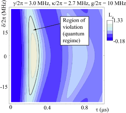
Figure 2: A violation of the extended Leggett-Garg inequality (15) for typical parameters in single-photon cavity QED experiments^2,3, using time-adjusted photon statistics. The parameters used here are: $\kappa/2\pi=$2.7 MHz, $g/2\pi=$10 MHz, and the variation of the detuning $\delta/2\pi$ can be up to 20 MHz. The violation of the inequality is indicated by the grey “island” inside the black contour line.

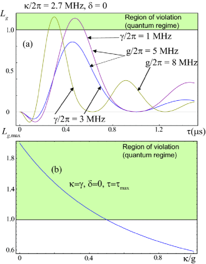
Figure 3: (a) The non-adjusted photon-counting statistics also exhibit a violation of the Leggett-Garg inequality (15). The combined effect of the atom polarization decay and the cavity decay rates ($\gamma/2\pi=3$ MHz and $\kappa/2\pi=2.7$ MHz), prevent a violation being seen in the data in ref. 1. However, a slight decrease in the polarization decay rate $\gamma$; or an increase in the coupling strength $g$, combined with the ultra-short laser pulses in ref. 1, should reveal a violation of the inequality (15). (b) Using the same model (without time-adjusted counting), one can estimate the ratio between the coupling strength $g$ and the dissipation ($\kappa$, $\gamma$) needed to observe a violation of (15). This is approximately given by the vacuum Rabi splitting VRS$\,=4g/(\kappa+\gamma)>4$. In (b) we have chosen $\kappa=\gamma$.

I.5.2 Extension of the Leggett-Garg Inequality

To further clarify the quantum signatures in these correlation functions, we turn to an extension¹⁵ of the Leggett-Garg inequality¹⁶. Recently, we derived our extended inequality based on measurements of the fluctuating current through a DQD device¹⁵. Since the current is essentially an invasive measurement, we showed that the inequality only applies for systems with a state space of three or less states, and under the assumption of irreversible transport into the right reservoir (see Methods). For the cavity QED system, these two assumptions become that of being in the single-excitation manifold, and the irreversible loss of photons once they leave the cavity, respectively. Thus, the current inequality of ref. 15,

$$|L_{I}(t)|\equiv|2\langle I(t+\tau)I(t)\rangle-\langle I(t+2\tau)I(t)\rangle|\leq\Gamma_{R}\langle I(t)\rangle,$$ (16)

becomes a second-order photon-correlation inequality,

$$|L_{g}(t)|\equiv|2g^{(2)}(t,t+\tau)-g^{(2)}(t,t+2\tau)|\leq{\langle a^{\dagger}(t)a(t)\rangle}^{-1}.$$ (17)

Superficially, this inequality is equivalent to the Leggett-Garg inequality in the stationary limit¹⁶. However, as mentioned above, the observation of a photon is an invasive measurement in terms of the cavity-atom state, and thus, strictly speaking, this inequality no longer can be discussed in terms of distinguishing theories obeying macroscopic realism from quantum mechanics: the original goal of the work of Leggett and Garg. Here this inequality only distinguishes quantum dynamics from those given by a classical rate equation. See the methods section, and ref. 15, for more details. Like the non-negative shot-noise feature, this inequality reveals a more nuanced way of understanding whether certain photon statistics have quantum characteristics, beyond those indicated by anti-bunching alone.

In Fig. 2, we show how the violation of this inequality occurs for a typical cavity QED experiment, using^1-4 $\kappa/2\pi=$2.7 MHz, $\gamma/2\pi=3$ MHz, $g=$10 MHz. As seen in Fig. 2, the violations of the inequality are easily observable and appear in a wide range of detuning $\delta$.

I.5.3 Extended inequality with standard photon statistics

One can also apply the extended¹⁵ Leggett-Garg inequality to the photon statistics without time-adjustment. In this case, a histogram of the photon counts as a function of time (after the initial excitation of the atom) is equivalent to the second-order correlation function of the atom-cavity system with one excitation and cavity decay, but no further time-dependent excitations. See refs. 1-4 for clear examples of such statistics.

Using a simple model of the Bochmann et al’s experiment¹ (using equations (1-3), and the initial state $\rho_{0}=|g,1\rangle\langle g,1|$), we have found that their experiment does not violate the inequality (15) (the bound is now set by the choice of initial state, see methods). A factor of two decrease in the atomic polarization decay rate, or a correspondingly stronger coupling strength, should reveal a violation. We illustrate this in Fig. 3a, again using their parameters; though we omit dephasing because of variations in coupling $g$. It is easy to see that a violation of (15) should be possible with minor improvements in system parameters. To give a more general bound for parameters which can cause a violation, in Fig. 3b we show the magnitude of the violation versus the cavity and atomic losses. This gives a bound on the Vacuum Rabi Splitting parameters needed to observe a violation of $2g/[(\gamma+\kappa)/2]>4$. Many realizations of cavity QED have parameters which exceed this (see, e.g., ref. 5). We therefore think that this inequality (15) is a useful addition to the toolbox one can use to test for quantum behavior in optical systems (see refs. 26,27 for reviews of other common tests).

II Discussion

We have shown how a simple adjustment of the output photon-detection statistics of a periodically-excited cavity QED system can be described by a non-equilibrium model, with an exact analogy to electron transport properties through a double quantum dot. This represents a unification of the fields of photon-counting statistics and electron-transport statistics. We then adapted several recent results from transport theory to describe or test the quantum nature of the photon-statistics being emitted from the cavity.

We emphasize that not only the current noise, but also the higher-order moments^28,29 can be examined with this time-adjusted scenario. Moreover, we point out that the same features could be observed in a circuit QED system, where the artificial atom (qubit) is periodically excited by some external means, and photons detected with a microwave photon counter³⁰.

II.1 ACKNOWLEDGMENTS

NL and YN-C contributed equally to this work. NL is supported by the RIKEN FPR program. YN-C is supported partially by the National Science Council of Taiwan under the grant number 98-2112-M-006-002-MY3. FN acknowledges partial support from the Laboratory of Physical Sciences, National Security Agency, Army Research Office, National Science Foundation grant No. 0726909, JSPS-RFBR contract No. 09-02-92114, Grant-in-Aid for Scientific Research (S), MEXT Kakenhi on Quantum Cybernetics, and Funding Program for Innovative R&D on S&T (FIRST).

III Methods

Effective feedback formalism. First, we describe the measurement of a single photon (which has leaked from the cavity and is incident on a photodetector) as $\mathcal{K}(dt)_{1}=\sqrt{dt}\,a$. The complementary operator to this one, which is applied when no photon is detected during the duration $dt$, is $\mathcal{K}(dt)_{2}=\sqrt{dt}\,a-(iH_{c}+\frac{1}{2}a^{\dagger}a)dt$. The feedback evolution which is then applied to the system, given the observation of a photon, is described by $\mathcal{O}[...]=|e\rangle\langle g|...|g\rangle\langle e|$; i.e. the atom is instantaneously and incoherently projected into its excited state. In general, this is not a trace-preserving evolution, as it is not a Liouvillian evolution, and is thus different from the class of feedback mechanisms described in refs. 17,18. Alternatively, one could assume a Liouvillian evolution according to the coherent dynamics of a laser pulse causing $\pi$-pulse/Rabi oscillations of the atom from its ground to excited state, via an operator $e^{-i\mathcal{Z}}$, $\mathcal{Z}=[\sigma_{x},...]$. However, in the limit when this transition is faster than all other dynamics, and we are in the single-excitation manifold, then it is equivalent to $\mathcal{O}[...]$.

The unnormalized density matrix following the detection of a photon at time $t$, and evolution due to feedback, is

$$\tilde{\rho}_{1}(t+dt)=\kappa\mathcal{O}a\rho(t)a^{\dagger}dt.$$

Our time-adjustment scheme implies that the time delay is far smaller (effectively zero) than the cavity decay time, and one can assume the fully Markovian master equation,

$$\dot{\rho}=-i[H_{c},\rho]+\kappa\mathcal{O}a\rho a^{\dagger}-\frac{\kappa}{2}\bigg{[}a^{\dagger}a\rho+\rho a^{\dagger}a\bigg{]}.$$

If the feedback is via the operator $\mathcal{O}[...]$, this is not a trace-preserving equation of motion. However, if we restrict ourselves to the single (lowest) excitation manifold, only the $\left|e,0\right\rangle$, $\left|g,1\right\rangle$, and $|g,0\rangle$ states are important. Then the feedback term becomes $\mathcal{O}a\rho a^{\dagger}=|e,0\rangle\langle g,1|\rho|g,1\rangle\langle e,0|$, and this truncated basis is trace-preserving, as the state $|e,1\rangle$ is decoupled from the equation of motion, giving $\mathrm{Tr}[\mathcal{O}a\rho a^{\dagger}]=\mathrm{Tr}[a\rho a^{\dagger}]=\langle g,1|\rho|g,1\rangle$.

Now the action of the instantaneous feedback is obvious, such that the state $|g,0\rangle$ in the photon-decay terms is decoupled from the single-excitation manifold. We can now write our equation of motion purely in the pseudo-spin two-state basis, defining $\tilde{\sigma}_{z}=|e,0\rangle\langle e,0|-|g,1\rangle\langle g,1|$,

$$\dot{\rho} = -i[\nu+\delta\tilde{\sigma}_{z}+g\tilde{\sigma}_{x},\rho]$$

$$+ \kappa\tilde{\sigma_{+}}\rho\tilde{\sigma_{-}}-\frac{\kappa}{2}\bigg{[}\tilde{\sigma_{-}}\tilde{\sigma_{+}}\rho+\rho\tilde{\sigma_{-}}\tilde{\sigma_{+}}\bigg{]},$$

where $\delta=\omega-\nu$ is the detuning between the atom and the cavity.

To achieve the above, we note the following points. First, the delay between measurement and feedback is instantaneous. In our case the delay is zero, as dictated by our adjustment of time intervals in the data set. Second, the feedback action (i.e., laser pulse) incoherently and instantaneously projects the system into the $|e,0\rangle$ state. This has recently been achieved by Bochmann et al.¹ using ultra-short laser pulses. Third, the photon detection is here assumed to be $100\%$ efficient. This can be effectively achieved by simply omitting the time intervals where no photons are detected.

Derivation of the extended Leggett-Garg inequality. In ref. 15, we extended the Leggett-Garg inequality to work under the conditions of invasive measurement, but with additional restrictions. We summarize and reformulate the proof of that inequality here, but now using the language of cavity-QED.

For the cavity-QED case, we posit that any photon-intensity measurements not conditioned by quantum dynamics obey

$$|L_{g}(t,t+\tau)|\equiv|2g^{(2)}(t,t+\tau)-g^{(2)}(t,t+2\tau)|\leq{\langle a^{\dagger}(t)a(t)\rangle}^{-1}.$$ (18)

In the language of an effective photon current, we can write this as

$$|L_{I}(t,t+\tau)| \equiv$$ (19)

$$|2\langle I_{\mathrm{ph}}(t+\tau)I_{\mathrm{ph}}(t)\rangle - \langle I_{\mathrm{ph}}(t+2\tau)I_{\mathrm{ph}}(t)\rangle|\leq\kappa\langle I_{\mathrm{ph}}\rangle,$$

where $\kappa$ is the rate of photons leaking from the cavity, $I_{\mathrm{ph}}(t)\equiv I_{\mathrm{ph}}(t=0)$ and $\langle I_{\mathrm{ph}}(t)\rangle$ is the average photon current of the initial state. Hereafter we omit the $t$ variable. In the master equation approach, the current operator translates into a “jump” super-operator, and equation (19) thus represents an inequality concerning transitions in the system, and not static properties. Thus it is obviously suitable for application to single-photon measurements, which give us information about a change in the state of the cavity-QED system. As described in the text, the photon current super-operator acts as before $\hat{I}_{\mathrm{ph}}[\rho]=\kappa\tilde{\sigma}^{+}\rho\tilde{\sigma}^{-}$, such that the average current is $\langle I_{\mathrm{ph}}\rangle=\mathrm{Tr}\left\{\hat{I}_{\mathrm{ph}}\rho\right\}$ and the correlation function of interest is obtained as $\langle I_{\mathrm{ph}}(\tau)I_{\mathrm{ph}}\rangle=\mathrm{Tr}\left\{\hat{I}_{\mathrm{ph}}e^{\mathcal{L}\tau}\hat{I}_{\mathrm{ph}}\rho_{0}\right\}$. For our time-adjusted case, the stationary distribution is chosen as the initial state. For the non-time-adjusted photon statistics, one chooses $\rho_{0}=|g,1\rangle\langle 1,g|$.

In these terms, the inequality expression can be written as $L_{I}(\tau)=\mathrm{Tr}\left\{\hat{I}_{\mathrm{ph}}\left(2e^{\mathcal{L}\tau}-e^{2\mathcal{L}\tau}\right)\hat{I}_{\mathrm{ph}}\rho_{0}\right\}.$ If the cavity-QED system contains no coherent quantum dynamics, $\hat{I}_{\mathrm{ph}}$ is the $3\times 3$ matrix with elements $\hat{I_{\mathrm{ph}}}_{\alpha\beta}=\kappa\delta_{\alpha,0}\delta_{\beta,\mathcal{P}}$, where the indices $0=|g,0\rangle,\mathcal{P}=|g,1\rangle,\mathcal{A}=|e,0\rangle$. Thus using the Chapman-Kolgomorov equation, we have

$$L_{I}(\tau)=\kappa^{2}P_{\mathcal{P}}(0)\bigg{[}\Omega_{\mathcal{P}0}\left(2-\Omega_{00}-\Omega_{\mathcal{P}\mathcal{P}}\right)-\Omega_{\mathcal{P}\mathcal{A}}\Omega_{\mathcal{A}0}\bigg{]}.$$

Where $\Omega$ represents the matrix elements of the propagator. For a general Markov stochastic matrix, $\Omega$, the maximum of $L_{I}$ is

$$\mathrm{max}\{L_{I}\}=2\kappa^{2}P_{\mathcal{P}}(0).$$

However, the rate equation form $\Omega(\tau)=\exp{\mathcal{L}\tau}$ furnishes us with a further constraint. Maximizing $L_{I}(\tau)$ with respect to time, from $\dot{L}_{I}=0$ and $\dot{\Omega}=\mathcal{L}\Omega$, we find that the maximum of $L_{I}$ occurs when $\Omega_{00}+\Omega_{\mathcal{P}\mathcal{P}}=1$ and $\Omega_{\mathcal{P}0}=1$, giving

$$\mathrm{max}\{L_{I}\}=\kappa^{2}P_{\mathcal{P}}(0)=\kappa\langle I_{ph}\rangle.$$

This result relies on the form of the jump operator and the absence of re-absorbtion of photons by the cavity, i.e. $\mathcal{L}_{\mathcal{P}0}=0$. These requirements mean that we must always be in the single-excitation regime, and that once a photon leaves the cavity and is measured, it cannot return. Fortunately, this is implicit in the definition of destructive photon measurement.

References

- (1) Bochmann, J., Mucke, M., Langfahl-Klabes, G., Erbel, C., Weber, B., Specht, H. P., Moehring, D. L. & Rempe, G. Fast excitation and photon emission of a single-atom-cavity system. Phys. Rev. Lett. 101, 223601 (2008).
- (2) Miller, R., Northup, T. E., Birnbaum, K. M., Boca, A., D. Boozer, A. & Kimble, H. J. Trapped atoms in cavity QED: coupling quantized light and matter. J. Phys. B 38, S551-S565 (2005).
- (3) McKeever, J., Boca, A., D. Boozer, A., Miller, R., Buck, J. R., Kuzmich, A. & Kimble, H. J. Deterministic generation of single photons from one atom trapped in a cavity. Science 303, 1992-1994 (2004).
- (4) Raimond, J. M., Brune, M. & Haroche, S. Manipulating quantum entanglement with atoms and photons in a cavity. Rev. Mod. Phys. 73, 565-582 (2001).
- (5) Khitrova, G., Gibbs, H. M., Kira, M., Koch, S. W. & Scherer, A. Vacuum Rabi splitting in semiconductors. Nature Physics 2, 81-90 (2006).
- (6) You, J. Q. & Nori, F. Superconducting circuits and quantum information. Phys. Today 58, No. 11, 42-47 (2005).
- (7) Schoelkopf, R. J. & Girvin, S. M. Wiring up quantum systems. Nature 451, 664-669 (2008).
- (8) Clarke, J. & Wilhelm, F. K. Superconducting quantum bits. Nature 453, 1031-1042 (2008).
- (9) Shchukin, V. A. & Bimberg, D. Spontaneous ordering of nanostructures on crystal surfaces. Rev. Mod. Phys. 71, 1125-1171 (1999).
- (10) van der Wiel, W. G., De Franceschi, S., Elzerman, J. M., Fujisawa, T., Tarucha, S. & Kouwenhoven, L. P. Electron transport through double quantum dots. Rev. Mod. Phys. 75, 1-22 (2003).
- (11) Ziegler, R., Bruder, C. & Schoeller, H. Transport through double quantum dots. Phys. Rev. B 62, 1961-1970 (2000).
- (12) Aleiner, I. L., Brouwer, P. W. & Glazman, L. I. Quantum effects in Coulomb blockade. Phys. Rep. 358, 309-440 (2002).
- (13) Levitov, L. S., Lee, H.-W. & Lesovik, G. B. Electron counting statistics and coherent states of electric current. J. Math. Phys. 37, 4845 (1996) .
- (14) Hayashi, T., Fujisawa, T., Cheong, H. D., Jeong, Y. H. & Hirayama, Y. Coherent manipulation of electronic states in a double quantum dot. Phys. Rev. Lett. 91, 226804 (2003).
- (15) Lambert, N., Emary, C., Chen, Y. N. & Nori, F. Distinguishing quantum and classical transport through nanostructures. arxiv:1002.3020 (2010).
- (16) Leggett, A. J. & Garg, A. Quantum mechanics versus macroscopic realism: Is the flux there when nobody looks? Phys. Rev. Lett. 54, 857-860 (1985).
- (17) Wiseman, H. M. & Milburn, G. J. Quantum Measurement and Control, Cambridge Univ. Press, Cambridge, UK (2010).
- (18) Reiner, J. E., Wiseman, H. M. & Mabuchi, H. Quantum jumps between dressed states: A proposed cavity-QED test using feedback. Phys. Rev. A. 67, 042106 (2003).
- (19) Scully, M. O. & Zubairy, M. S. Quantum Optics, Cambridge Univ. Press, Cambridge, UK (1997).
- (20) Brandes, T. Coherent and collective quantum optical effects in mesoscopic systems. Phys. Rep. 408, 315-474 (2005).
- (21) Lambert, N. & Nori, F. Detecting quantum-coherent nanomechanical oscillations using the current-noise spectrum of a double quantum dot. Phys. Rev. B 78, 214302 (2008).
- (22) Elattari, B. & Gurvitz, S. A. Shot noise in coupled dots and the “fractional charges”. Phys. Lett. A 292, 289-294 (2002).
- (23) Hershfield, S., Davies, J. H., Hyldgaard, P., Standon, C. J. & Wilkins, J. W. Zero-frequency current noise for the double-tunnel-junction Coulomb blockade. Phys. Rev. B 47, 1967-1979 (1993).
- (24) Barthold, P., Hohls, F., Maire, N., Pierz, K. & Haug, R. J. Enhanced shot noise in tunneling through a stack of coupled quantum dots. Phys. Rev. Lett. 96, 246804 (2006).
- (25) Kießlich, G., Schöll, E., Brandes, T., Hohls, F. & Haug, R. J. Noise enhancement due to quantum coherence in coupled quantum dots. Phys. Rev. Lett. 99, 206602 (2007).
- (26) Miranowicz, A., Bajer, J., Matsueda, H., Wahiddin, M. R. B. & Tanas, R. Comparative study of photon antibunching of non-stationary fields. J. Opt. B, 511-516 (1999).
- (27) Miranowicz, A., Bartkowiak, M., Wang, X., Liu, Y.X. & Nori, F. Testing nonclassicality in multimode fields: a unified derivation of classical inequalities. Phys. Rev. A 82, 013824 (2010).
- (28) Fujisawa, T., Hayashi, T., Tomita, R. & Hirayama, Y. Bidirectional counting of single electrons. Science 312, 1634-1636 (2006).
- (29) Flindt, C., Fricke, C., Hohls, F., Novotny, T., Netocny, K., Brandes, T. & Haug, R. J. Universal oscillations in counting statistics. Proc. Natl. Acad. Sci. U.S.A. 106, 10116-10119 (2009).
- (30) Romero, G., Garcia-Ripoll, J. J. & Solano, E. Microwave photon detector in circuit QED. Phys. Rev. Lett. 102, 173602 (2009).