Optimal transportation, topology and uniqueness

Abstract

The Monge-Kantorovich transportation problem involves optimizing with respect to a given a cost function. Uniqueness is a fundamental open question about which little is known when the cost function is smooth and the landscapes containing the goods to be transported possess (non-trivial) topology. This question turns out to be closely linked to a delicate problem (# 111) of Birkhoff [14]: give a necessary and sufficient condition on the support of a joint probability to guarantee extremality among all measures which share its marginals. Fifty years of progress on Birkhoff’s question culminate in Hestir and Williams’ necessary condition which is nearly sufficient for extremality; we relax their subtle measurability hypotheses separating necessity from sufficiency slightly, yet demonstrate by example that to be sufficient certainly requires some measurability. Their condition amounts to the vanishing of the measure $\gamma$ outside a countable alternating sequence of graphs and antigraphs in which no two graphs (or two antigraphs) have domains that overlap, and where the domain of each graph / antigraph in the sequence contains the range of the succeeding antigraph (respectively, graph). Such sequences are called numbered limb systems. We then explain how this characterization can be used to resolve the uniqueness of Kantorovich solutions for optimal transportation on a manifold with the topology of the sphere.

1 Introduction

This survey weaves together two themes: the first is Monge’s 1781 problem [81] of transporting mass from a landscape $X$ to a landscape $Y$ so as to minimize the average cost $c(x,y)$ per unit transported; the second is Birkhoff’s 1948 problem [14] of characterizing extremality among doubly stochastic measures on the unit square.

The first problem has become classical in the calculus of variations; it has deep connections to analysis [98] [73] [74] [30] [51], geometry [83] [29] [95] [71] [70] [104] [79] [63], dynamics [7] [10] [59] [82] and nonlinear partial differential equations [18] [20] [21] [36] [42] [72] [102], as well as applications in physics [38] [97] [75], statistics [88], engineering [15] [16] [57] [86] [107], atmospheric modeling [34] [87] [35] [33], and economics [24] [25] [41] [27] [49]. The second is a problem in functional analysis, at the junction between measure theory and convex geometry. It is not evident that either involves differential topology.

The two problems are linked by Kantorovich’s reformulation of Monge’s nonlinear minimization as an (infinite-dimensional) linear program [60] [61]. In this framework, existence of solutions became straightforward for any continuous cost $c\in C(X\times Y)$. Still, fifty more years would elapse before the optimal volume-preserving map between two arbitrary domains sought by Monge was constructed for the Euclidean distance $c(x,y)=|x-y|$ in [4] [22] and [99]. Evans and Gangbo had already solved the analogous problem with the domains replaced by disjoint Lipschitz continuous probability densities [42], while Sudakov’s earlier construction [96] required a claim which turned out to be true only two in dimensions [4] [12]; see [23] [26] [12] for simplifications and [44] [6] [9] [47] for extensions. Uniqueness fails in this context [54] [45]. In the meantime both Monge and Kantorovich problems were found to enjoy unique solutions for strictly convex costs such as $c(x,y)=|x-y|^{p}/p$, with $p=2$ [17] [18] [31] [32] and $p>1$ [19] [53] [54] [89] [90]. A general criterion for existence and uniqueness of optimal maps was identified by Gangbo [52] and Levin [66], building on works of those cited above. For any pair of destinations $y_{1}\neq y_{2}$ in $Y$, it prohibits the function

$$x\in X\longmapsto c(x,y_{1})-c(x,y_{2})$$ (1)

from having critical points on $X$. Strictly convex functions $c(x,y)=h(x-y)$ on $X=Y=\mathbf{R}^{n}$ [19] [53] satisfy this condition — called the twist criterion in [104] — but no differentiable cost $c\in C^{1}(X\times Y)$ satisfies it on any compact manifold $X$ without boundary. Although terrestrial transportation takes place on the sphere, there are few theorems set in topologies other than the ball — not to speak of the more exotic landscapes which arise naturally in some applications. Spherical examples typically show that uniqueness of Kantorovich solutions holds even though Monge solutions fail to exist [55]. Building on these developments, one of the goals of this article is to expose a criterion for uniqueness of Kantorovich solutions which works equally well on the sphere and the ball [27]. Called the subtwist by Chiappori McCann and Nesheim, this criterion depends on the Morse structure of the cost globally: it permits the function (1) to have up to two critical points on $X$ — a unique global minimum and a unique global maximum. Unfortunately, this cannot be satisfied in more exotic topologies such as the $k$-holed torus ($k\geq 1$), where uniqueness remains a tantalizing open question. Our discussion is predicated on global differentiability of the cost, since a wide variety of existence and uniqueness results concerning optimal solutions to the Monge-Kantorovich problem have been established for costs with singular sets — including distances in Riemannian [28] [77] [46], sub-Riemannian [5] [2] [50] and Alexandrov [11] spaces, and the mechanical actions arising from Tonelli Lagrangians [9] [43].

The proof that the subtwist condition is sufficient for uniqueness relies on progress in Birkhoff’s problem of characterizing extremal doubly stochastic measures on the square. This problem is esoteric and subtle: although still not completely resolved, substantial results have been obtained in the six decades since it was posed [39] [67] [69] [8] [58]. Highlights are surveyed below.

The literature surrounding Birkhoff’s problem is modest, compared to the recent explosion of research on the Monge-Kantorovich transportation problem. We expect the main interest of this article will therefore lie in its connection to the latter developments. For simplicity of exposition, however, we postpone a further description of these connections to section 5. The earlier sections are devoted to Birkhoff’s problem and the issues surrounding it. Although less familiar than the Monge-Kantorovich theory to most of our readership, the developments surveyed are elementary yet powerful; they require nothing more sophisticated than measure theory to discuss. Readers in need of motivation — or those interested primarily in optimal transportation — are encouraged to skip directly to Theorem 5.1 for a preview of the intended application.

2 Extremal doubly stochastic measures

An $n\times n$ doubly stochastic matrix refers to a matrix of non-negative entries whose columns and rows each sum to $1$. The doubly stochastic matrices form a convex subset of all $n\times n$ matrices — in fact a convex polytope, whose extreme points are in bijective correspondence with the $n!$ permutations on $n$-letters, according to Birkhoff [13] and von Neumann [105]. For example, the $3\times 3$ doubly stochastic matrices,

$$\left(\begin{matrix}s&t&1-s-t\\ u&v&1-u-v\\ 1-s-u&1-t-v&s+t+u+v-1\\ \end{matrix}\right)$$

form a 4-dimensional polytope with 6 vertices. Shortly after proving this characterization, Birkhoff [14, Problem 111] initiated the search for a infinite-dimensional generalization, thus stimulating a line of research which remains fruitful even today.

A doubly stochastic measure on the square refers to a non-negative Borel probability measure on $[0,1]^{2}$ whose horizontal and vertical marginals both coincide with Lebesgue measure $\lambda$ on $[0,1]$. The set of doubly stochastic measures forms a convex set we denote by $\Gamma(\lambda,\lambda)$ (which is weak-$*$ compact in the Banach space dual to continuous functions $C([0,1]^{2})$ normed by their suprema $\|\cdot\|_{\infty}$). A measure is said to be extremal in $\Gamma(\lambda,\lambda)$ if it cannot be decomposed as a convex combination $\gamma=(1-t)\gamma_{0}+t\gamma_{1}$ with $0<t<1$ and $0\leq\gamma_{0}\neq\gamma_{1}\in\Gamma(\lambda,\lambda)$. Since the Krein-Milman theorem asserts that convex combinations of extreme points are dense (in any compact convex subset of a topological vector space, Figure 1), it is natural to want to characterize the extreme points of $\Gamma(\lambda,\lambda)$. Another motivation for such a characterization is that every continuous linear functional on $\Gamma(\lambda,\lambda)$ is minimized at an extreme point. Whether or not this extremum is uniquely attained can be an interesting question, as in the optimal transportation context: in Figure 1 the horizontal coordinate is minimized at a single point but maximized at two extreme points (and along the segment joining them).

Figure 1: Krein-Milman asserts a compact convex set $\mathbf{K}$ can be reconstructed from its extreme points (denoted here by solid circles $\bullet$ and solid lines $\boldsymbol{-}$).

Motivated by the optimization problems already mentioned, we prefer to formulate the question in slightly greater generality, by replacing the two copies of $([0,1],\lambda)$ with probability spaces $(X,\mu)$ and $(Y,\nu)$, where $X$ and $Y$ are each subsets of a complete separable metric space, and $\mu$ and $\nu$ are Borel probability measures on $X$ and $Y$ respectively. This widens applicability of the answer to this question without increasing its difficulty. Letting $\Gamma(\mu,\nu)$ denote the Borel probability measures on $X\times Y$ having $\mu$ and $\nu$ for marginals, we wish to characterize the extreme points of the convex set $\Gamma(\mu,\nu)$. Ideally, as in the finite-dimensional case, this characterization would be given in terms of some geometrical property of the support of the measure $\gamma$ in $X\times Y$. Indeed, if $\mu=\sum_{i=1}^{m}m_{i}\delta_{x_{i}}$ and $\nu=\sum_{j=1}^{n}n_{j}\delta_{y_{j}}$ are finite, our problem reduces to characterizing the extreme points of the convex set ${\cal A}$ of $m\times n$ matrices with prescribed column and row sums:

$${\cal A}=\{a_{ij}\geq 0\mid m_{i}=\sum_{j=1}^{n}a_{ij},\sum_{i=1}^{m}a_{ij}=n_{j}\}.$$

A matrix $(a_{ij})$ is well-known to be extremal in ${\cal A}$ if and only if it is acyclic, meaning for every sequence $a_{i_{1}j_{1}},\ldots,a_{i_{k}j_{k}}$ of non-zero entries occupying $k\geq 2$ distinct columns and $k$ distinct rows, the product $a_{i_{1}j_{2}}\ldots a_{i_{k-1}j_{k}}a_{i_{k}j_{1}}$ must vanish — see Figure 2 or Denny [37], where the terminology aperiodic is used. Similarly, a set $S\subset X\times Y$ is acyclic if for every $k\geq 2$ distinct points $\{x_{1},\ldots,x_{k}\}\subset X$ and $\{y_{1},\ldots,y_{k}\}\subset Y$, at least one of the pairs $(x_{1}y_{1}),(x_{1},y_{2}),(x_{2},y_{2}),\ldots,(x_{k-1},y_{k}),(x_{k},y_{k}),(x_{k},y_{1})$ lies outside of $S$.

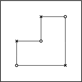
Figure 2: In an acyclic matrix the product of x’s and o’s must vanish.

A functional analytic characterization of extremality was supplied by Douglas [39] and by Lindenstrauss [67]: it asserts that $\gamma$ is extremal in $\Gamma(\mu,\nu)$ if and only if $L^{1}(X,d\mu)\oplus L^{1}(Y,d\nu)$ is dense in $L^{1}(X\times Y,d\gamma)$. Although this result is a wonderful starting point, it is not quite the characterization we desire for applications, since it is not easily expressed in terms of the geometry of the support of $\gamma$. Significant further progress was made by Beneš and Štěpán, who showed every extremal doubly stochastic measure vanishes outside some acyclic subset $S\subset X\times Y$ [8]. Hestir and Williams refined this condition, showing that it becomes sufficient under an additional Borel measurability hypothesis which, unfortunately, is not always satisfied [58]. Some of the subtleties of the problem were indicated already by Losert’s counterexamples [69]. The difficulty of the problem resides partly in the fact that any geometrical characterization of optimality must be invariant under arbitrary measure-preserving transformations applied independently to the horizontal (abscissa) and vertical (ordinate) variables.

In the next two sections we review this line of research, clarifying the nature of the gap separating necessity from sufficiency and pointing out that it can be narrowed slightly by replacing the Borel $\sigma$-algebra with suitably adapted measure-completions. We give a self-contained proof of that part of the theory which is needed to resolved the uniqueness of optimal transportation with respect to a smooth cost on the sphere. This application was first developed in an economic context by Chiappori, McCann, and Nesheim [27], and forms the subject of the final section of the present manuscript.

3 Measures on graphs are push-forwards

Before recalling the characterization of interest, let us develop a bit of notation in a simpler setting, and a key argument that we shall require. Impatient or knowledgeable readers can proceed directly to the final sections below, referring back to the present section only as needed.

Let $X$ and $Y$ be subsets of complete separable metric spaces, and fix a non-negative Borel measure $\mu$ on $X$. Suppose $f:X\longrightarrow Y$ is $\mu$-measurable, meaning $f^{-1}(B)$ is in the $\sigma$-algebra completion of the Borel subsets of $X$ with respect to the measure $\mu$, whenever $B$ is relatively Borel in $Y$. Then a Borel measure on $Y$ is induced, denoted $f_{\#}\mu$ and called the push-forward of $\mu$ through $f$, and given by

$$(f_{\#}\mu)[B]:=\mu[f^{-1}(B)]$$ (2)

for each Borel $B\subset Y$. Defining the projections $\pi^{X}(x,y)=x$ and $\pi^{Y}(x,y)=y$ on $X\times Y$, this notation permits the horizontal and vertical marginals of a measure $\gamma\geq 0$ on $X\times Y$ to be expressed as $\pi^{X}_{\#}\gamma$ and $\pi^{Y}_{\#}\gamma$ respectively.

The next lemma shows that any measure supported on a graph can be deduced from its horizontal marginal. It improves on Lemma 2.4 of [55] and various other antecedents, by using an argument from Villani’s Theorem 5.28 [104] to extract $\mu$-measurability of $f$ as a conclusion rather that a hypothesis. As work of, e.g., Hestir and Williams [58] implies, although measures on graphs are extremal in $\Gamma(\mu,\nu)$, the converse is far from being true; this peculiarity is an inevitable consequence of the infinite divisibility of $(X,\mu)$.

Lemma 3.1 (Measures on graphs are push-forwards)

Let $X$ and $Y$ be subsets of complete separable metric spaces, and $\gamma\geq 0$ a $\sigma$-finite Borel measure on the product space $X\times Y$. Denote the horizontal marginal of $\gamma$ by $\mu:=\pi_{\#}^{X}\gamma$. If $\gamma$ vanishes outside the graph of $f:X\longrightarrow Y$, meaning $\{(x,y)\in X\times Y\mid y\neq f(x)\}$ has zero outer measure, then $f$ is $\mu$-measurable and $\gamma=(id_{X}\times f)_{\#}\mu$, where $id_{X}\times f$ denotes the map $x\in X\longmapsto(x,f(x))\in X\times Y$.

Proof. Since outer-measure is subadditive, it costs no generality to assume the subsets $X$ and $Y$ are in fact complete and separable, by extending $\gamma$ in the obvious (minimal) way. Any $\sigma$-finite Borel measure $\gamma$ is regular and $\sigma$-compact on a complete separable metric space; e.g. p. 255 of [40] or Theorem I-55 of [103]. Since $\gamma$ vanishes outside $\mathop{\rm Graph}(f):=\{(x,f(x))\mid x\in X\}$, there is an increasing sequence of compact sets $K_{i}\subset K_{i+1}\subset\mathop{\rm Graph}(f)$ whose union $K_{\infty}=\lim_{i\to\infty}K_{i}$ contains the full mass of $\gamma$. Compactness of $K_{i}\subset\mathop{\rm Graph}(f)$ implies continuity of $f$ on the compact projection $X_{i}:=\pi^{X}(K_{i})$. Thus the restriction $f_{\infty}$ of $f$ to $X_{\infty}:=\pi^{X}(K_{\infty})$ is a Borel map whose graph $K_{\infty}=\mathop{\rm Graph}(f_{\infty})$ is a $\sigma$-compact set of full measure for $\gamma$. We now verify that $\gamma$ and $(id_{X_{\infty}}\times f_{\infty})_{\#}\mu$ assign the same mass to each Borel rectangle $U\times V\subset X\times Y$. Since $(U\times V)\cap\mathop{\rm Graph}(f_{\infty})=((U\cap f_{\infty}^{-1}(V))\times Y)\cap\mathop{\rm Graph}(f_{\infty})$ we find

$$\gamma(U\times V) = \gamma((U\cap f_{\infty}^{-1}(V))\times Y)$$

$$= \mu(U\cap f_{\infty}^{-1}(V)),$$

proving $\gamma=(id_{X_{\infty}}\times f_{\infty})_{\#}\mu$. Taking $U=X\setminus X_{\infty}$ and $V=Y$ shows $X\setminus X_{\infty}$ is $\mu$-negligible. Since $id_{X}\times f$ differs from the Borel map $id_{X_{\infty}}\times f_{\infty}$ only on the $\mu$-negligible complement of the $\sigma$-compact set $X_{\infty}$, we conclude $f$ is $\mu$-measurable and $\gamma=(id_{X}\times f)_{\#}\mu$ as desired.   

The preceding lemma shows that any measure concentrated on a graph is uniquely determined by its marginals; $\gamma$ is therefore extremal in $\Gamma(\pi^{X}_{\#}\gamma,\pi^{Y}_{\#}\gamma)$. As the results of the next section show, the converse is far from being true.

4 Numbered limb systems and extremality

In this section we adapt Hestir and Williams [58] notion of a numbered limb system — also called an axial forest or a limb numbering system — to $X\times Y$. Using the axiom of choice, Hestir and Williams deduced from the acyclicity condition of Beneš and Štěpán [8] that each extremal doubly stochastic measure vanishes outside some numbered limb system. Conversely, they showed that vanishing outside a numbered limb system is sufficient to guarantee extremality of a doubly stochastic measure, provided the graphs (and antigraphs) comprising the system are Borel subsets of the square. Our main theorem gives a new proof of this converse in the more general setting of subsets $X\times Y$ of complete separable metric spaces, and under a slightly weaker measurability hypothesis on the graphs and antigraphs. A simple example shows that some measurability hypothesis is nevertheless required. In the next and final section, we shall see how this converse relates to the question of uniqueness in optimal transportation.

Given a map $f:D\longrightarrow Y$ on $D\subset X$, we denote its graph, domain, range, and the graph of its (multivalued) inverse by

$$\mathop{\rm Graph}(f):= \{(x,f(x))\mid x\in D\},$$

$$\mathop{\rm Dom}f:= \pi^{X}(\mathop{\rm Graph}(f)) =D,$$

$$\mathop{\rm Ran}f:= \phantom{=}\pi^{Y}(\mathop{\rm Graph}(f)),$$

$$\mathop{\rm Antigraph}(f):= \{(f(x),x)\mid x\in\mathop{\rm Dom}f\} \subset Y\times X.$$

More typically, we will be interested in the $\mathop{\rm Antigraph}(g)\subset X\times Y$ of a map $g:D\subset Y\longrightarrow X$.

Figure 3: The subsets $I_{k}$ need not be connected; in this numbered limb system they are represented as connected sets for visual convenience only.

Definition 4.1 (Numbered limb system)

Let $X$ and $Y$ be Borel subsets of complete separable metric spaces. A relation $S\subset X\times Y$ is a numbered limb system if there is a countable disjoint decomposition of $X=\cup_{i=0}^{\infty}I_{2i+1}$ and of $Y=\cup_{i=0}^{\infty}I_{2i}$ with a sequence of maps $f_{2i}:\mathop{\rm Dom}(f_{2i})\subset Y\longrightarrow X$ and $f_{2i+1}:\mathop{\rm Dom}(f_{2i+1})\subset X\longrightarrow Y$ such that $S=\cup_{i=1}^{\infty}\mathop{\rm Graph}(f_{2i-1})\cup\mathop{\rm Antigraph}(f_{2i})$, with $\mathop{\rm Dom}(f_{k})\cup\mathop{\rm Ran}(f_{k+1})\subset I_{k}$ for each $k\geq 0$. The system has (at most) $N$ limbs if $\mathop{\rm Dom}(f_{k})=\emptyset$ for all $k>N$.

Notice the map $f_{0}$ is irrelevant to this definition though $I_{0}$ is not; we may always take $\mathop{\rm Dom}(f_{0})=\emptyset$, but require $\mathop{\rm Ran}(f_{1})\subset I_{0}$. The point is the following theorem and its corollary, which extends and relaxes the result proved by Hestir and Williams for Lebesgue measure $\mu=\nu=\lambda$ on the interval $X=Y=[0,1]$. In it, $\Gamma(\mu,\nu)$ denotes the set of non-negative Borel measures on $X\times Y$ having $\mu=\pi^{X}_{\#}\gamma$ and $\nu=\pi^{Y}_{\#}\gamma$ for marginals. As in the preceding lemma, we say $\gamma$ vanishes outside of $S\subset X\times Y$ if $\gamma$ assigns zero outer measure to the complement of $S$ in $X\times Y$.

Theorem 4.2 (Numbered limb systems yield unique correlations)

Let $X$ and $Y$ be subsets of complete separable metric spaces, equipped with $\sigma$-finite Borel measures $\mu$ on $X$ and $\nu$ on $Y$. Suppose there is a numbered limb system $S=\cup_{i=1}^{\infty}\mathop{\rm Graph}(f_{2i-1})\cup\mathop{\rm Antigraph}(f_{2i})$ with the property that $\mathop{\rm Graph}(f_{2i-1})$ and $\mathop{\rm Antigraph}(f_{2i})$ are $\gamma$-measurable subsets of $X\times Y$ for each $i\geq 1$ and for every $\gamma\in\Gamma(\mu,\nu)$ vanishing outside of $S$. If the system has finitely many limbs or $\mu[X]<\infty$, then at most one $\gamma\in\Gamma(\mu,\nu)$ vanishes outside of $S$. If such a measure exists, it is given by $\gamma=\sum_{k=1}^{\infty}\gamma_{k}$ where

$$\gamma_{2i-1}=(id_{X}\times f_{2i-1})_{\#}\eta_{2i-1}, \gamma_{2i}=(f_{2i}\times id_{Y})_{\#}\eta_{2i},$$ (3)

$$\eta_{2i-1}=\Big{(}\mu-\pi^{X}_{\#}\gamma_{2i}\big{)}\Big{|}_{\mathop{\rm Dom}f_{2i-1}}, \eta_{2i}=\Big{(}\nu-\pi^{Y}_{\#}\gamma_{2i+1}\Big{)}\Big{|}_{\mathop{\rm Dom}f_{2i}}.$$ (4)

Here $f_{k}$ is measurable with respect to the $\eta_{k}$ completion of the Borel $\sigma$-algebra. If the system has $N<\infty$ limbs, $\gamma_{k}=0$ for $k>N$, and $\eta_{k}$ and $\gamma_{k}$ can be computed recursively from the formulae above starting from $k=N$.

Proof. Let $S=\cup_{i=1}^{\infty}\mathop{\rm Graph}(f_{2i-1})\cup\mathop{\rm Antigraph}(f_{2i})$ be a numbered limb system whose complement has zero outer measure for some $\sigma$-finite measure $0\leq\gamma\in\Gamma(\mu,\nu)$. This means that $I_{k}\supset\mathop{\rm Dom}f_{k}$ gives a disjoint decomposition of $X=\cup_{i=0}^{\infty}I_{2i+1}$ and of $Y=\cup_{i=0}^{\infty}I_{2i}$, and that $\mathop{\rm Ran}(f_{k})\subset I_{k-1}$ for each $k\geq 1$. Assume moreover, that $\mathop{\rm Graph}(f_{2i})$ and $\mathop{\rm Antigraph}(f_{2i-1})$ are $\gamma$-measurable for each $i\geq 1$. We wish to show $\gamma$ is uniquely determined by $\mu$, $\nu$ and $S$.

The graphs $\mathop{\rm Graph}(f_{2i-1})$ are disjoint since their domains $I_{2i-1}$ are disjoint, and the antigraphs $\mathop{\rm Antigraph}(f_{2i})$ are disjoint since their domains $I_{2i}$ are. Moreover, $\mathop{\rm Graph}(f_{2i-1})$ is disjoint from $\mathop{\rm Antigraph}(f_{2j})$ for all $i,j\geq 1$: $\mathop{\rm Ran}(f_{2i-1})\subset I_{2i-2}$ prevents $\mathop{\rm Graph}(f_{2i-1})$ from intersecting $\mathop{\rm Antigraph}(f_{2j-2})$ unless $j=i$ since the domains $I_{2j-2}$ are disjoint, and $\mathop{\rm Graph}(f_{2i-1})$ cannot intersect $\mathop{\rm Antigraph}(f_{2i-2})$ since $\mathop{\rm Dom}(f_{2i-1})\subset I_{2i-1}$ is disjoint from $\mathop{\rm Ran}(f_{2i-2})\subset I_{2i-3}$.

Let $\gamma_{k}$ denote the restriction of $\gamma$ to $\mathop{\rm Antigraph}(f_{k})$ for $k$ even and to $\mathop{\rm Graph}(f_{k})$ for $k$ odd. Then $\gamma=\sum\gamma_{k}$ by our measurability hypothesis, and $\gamma_{k}$ restricts to a Borel measure on $X\times\mathop{\rm Dom}f_{k}$ if $k$ is even, and on $\mathop{\rm Dom}f_{k}\times Y$ if $k$ odd. Defining the marginal projections $\mu_{k}=\pi_{\#}^{X}\gamma_{k}$ and $\nu_{k}=\pi_{\#}^{Y}\gamma_{k}$, setting $\eta_{k}=\nu_{k}$ if $k$ even and $\eta_{k}=\mu_{k}$ if $k$ odd yields (3) and the $\eta_{k}$-measurability of $f_{k}$ immediately from Lemma 3.1. Since $\nu_{2i}$ vanishes outside $\mathop{\rm Dom}f_{2i}$, from $\nu=\sum_{k=1}^{\infty}\nu_{k}$ we derive $\nu_{2i}=(\nu-\sum_{k\neq 2i}\nu_{k})|_{\mathop{\rm Dom}f_{2i}}$. For $k$ even, $\nu_{k}$ vanishes outside $\mathop{\rm Dom}f_{k}\subset I_{k}$, while for $k$ odd, $\nu_{k}$ vanishes outside $\mathop{\rm Ran}f_{k}\subset I_{k-1}$, which is disjoint from $\mathop{\rm Dom}f_{2i}$ unless $k=2i+1$. Thus $\eta_{2i}=(\nu-\nu_{2i+1})|_{\mathop{\rm Dom}f_{2i}}$. The formula (4) for $\eta_{2i-1}$ follows from similar considerations.

It remains to show the representation (3)–(4) specifies $(\gamma_{k},\eta_{k})$ uniquely for all $k\geq 1$, and hence determines $\gamma=\sum\gamma_{k}$ uniquely. If the system has $N<\infty$ limbs, $I_{k}=\emptyset$ for $k>N$ and hence $\gamma_{k}=0$. We can compute $\eta_{k}$ and $\gamma_{k}$ starting with $k=N$, and then recursively from the formulae above for $k=N-1,N-2,\ldots,1$, so the formulae represent $\gamma$ uniquely. If instead $S$ has countably many limbs, suppose there are two finite Borel measures $\gamma$ and $\bar{\gamma}$ vanishing outside of $S$ and having the same marginals $\mu$ and $\nu$. For each $k\geq 1$, recall that

$$K_{k}:=\left\{\begin{array}[]{lc}\mathop{\rm Graph}(f_{k})&k\ \mathrm{odd,}\\ \mathop{\rm Antigraph}(f_{k})&k\ \mathrm{even,}\end{array}\right.$$

is measurable with respect to both $\gamma$ and $\bar{\gamma}$. Given $\epsilon>0$, take $N$ large enough so that both $\gamma$ and $\bar{\gamma}$ assign mass less than $\epsilon$ to $\cup_{k=N}^{\infty}K_{k}$. Set $\gamma_{k}=\gamma|_{K_{k}}$ and $\bar{\gamma}_{k}=\bar{\gamma}|_{K_{k}}$ and denote their marginals by $(\mu_{k},\nu_{k})=(\pi^{X}_{\#}\gamma_{k},\pi^{Y}_{\#}\gamma_{k})$ and $(\bar{\mu}_{k},\bar{\nu}_{k})=(\pi^{X}_{\#}\bar{\gamma}_{k},\pi^{Y}_{\#}\bar{\gamma}_{k})$. Observe that both $\gamma^{\epsilon}:=\sum_{k=1}^{N}\gamma_{k}$ and $\bar{\gamma}^{\epsilon}:=\sum_{k=1}^{N}\bar{\gamma}_{k}$ are concentrated on the same numbered limb system; it has finitely many limbs, and the differences $\delta\mu^{\epsilon}=\sum_{k=1}^{N}(\bar{\mu}_{k}-\mu_{k})$ and $\delta\nu^{\epsilon}=\sum_{k=1}^{N}(\bar{\nu}_{k}-\nu_{k})$ between the marginals of $\gamma^{\epsilon}$ and $\bar{\gamma}^{\epsilon}$ have total variation at most $2\epsilon$. Since the $\delta\mu_{2i-1}=\bar{\mu}_{2i-1}-\mu_{2i-1}$ are mutually singular, as are the $\delta\nu_{2i}=\bar{\nu}_{2i}-\nu_{2i}$, we find the sum of the total variations of

$$\delta\eta_{k}:=\left\{\begin{array}[]{cc}\bar{\mu}_{k}-\mu_{k}&k\ \mathrm{odd,}\\ \bar{\nu}_{k}-\nu_{k}&k\ \mathrm{even,}\end{array}\right.$$

is bounded: $\sum_{k=1}^{N}\|\delta\eta_{k}\|_{TV(\mathop{\rm Dom}f_{k})}<4\epsilon$. Using (3) to derive

$$\|\bar{\gamma}_{k}-\gamma_{k}\|_{TV(X\times Y)} = \left\{\begin{array}[]{cc}\|(id_{X}\times f_{k})_{\#}\delta\eta_{k}\|_{TV(X\times Y)}&k\ \mathrm{odd,}\\ \|(f_{k}\times id_{Y})_{\#}\delta\eta_{k}\|_{TV(X\times Y)}&k\ \mathrm{even,}\end{array}\right.$$

$$= \|\delta\eta_{k}\|_{TV(\mathop{\rm Dom}f_{k})}$$

and summing on $k$ yields $\|\bar{\gamma}^{\epsilon}-\gamma^{\epsilon}\|_{TV(X\times Y)}<4\epsilon$. Since $\gamma^{\epsilon}\rightarrow\gamma$ and $\bar{\gamma}^{\epsilon}\rightarrow\bar{\gamma}$ as $\epsilon\rightarrow 0$, we conclude $\bar{\gamma}=\gamma$ to complete the uniqueness proof.   

As in Hestir and Williams [58], the uniqueness theorem above implies extremality as an immediate consequence.

Corollary 4.3 (Sufficient condition for extremality)

Let $X$ and $Y$ be subsets of complete separable metric spaces, equipped with $\sigma$-finite Borel measures $\mu$ on $X$ and $\nu$ on $Y$. Suppose there is a numbered limb system $S=\cup_{i=1}^{\infty}\mathop{\rm Graph}(f_{2i-1})\cup\mathop{\rm Antigraph}(f_{2i})$ with the property that $\mathop{\rm Graph}(f_{2i-1})$ and $\mathop{\rm Antigraph}(f_{2i})$ are $\gamma$-measurable subsets of $X\times Y$ for each $i\geq 1$, for every $\gamma\in\Gamma(\mu,\nu)$ vanishing outside of $S$. If the system has finitely many limbs or $\mu[X]<\infty$, then any measure $\gamma\in\Gamma(\mu,\nu)$ vanishing outside of $S$ is extremal in the convex set $\Gamma(\mu,\nu)$.

Proof. Suppose a measure $\gamma\in\Gamma(\mu,\nu)$ vanishes outside a numbered limb system $S$ satisfying the hypotheses of the corollary. If $\gamma=(1-t)\gamma_{0}+t\gamma_{1}$ with $\gamma_{0},\gamma_{1}\in\Gamma(\mu,\nu)$ and $0<t<1$, then $\gamma\geq\gamma_{0}$ and $\gamma\geq\gamma_{1}$, so both $\gamma_{0}$ and $\gamma_{1}$ vanish outside of $S$. According to Theorem 4.2, they are uniquely determined by $S$ and their marginals, hence $\gamma_{0}=\gamma_{1}$ to establish the corollary.   

The following example confirms that a measurability gap still remains between the necessary and sufficient conditions for extremality. It is a close variation on the standard example of a non-Lebesgue measurable set from real analysis. Together with the lemma and theorem preceding, this example makes clear that measurability is required only to allow the graphs to be separated from each other and from the antigraphs in an additive way.

Example 4.4 (An acyclic set supporting non-extremal measures)

Let $\lambda$ denote Lebesgue measure and define the maps $f_{0}(x)=x$ and $f_{1}(x)=x+\sqrt{2}$ (mod 1) on the unit interval $X=Y=[0,1]$. Notice $\mathop{\rm Graph}(f_{i})\subset[0,1]^{2}$ supports the doubly stochastic measure $\gamma_{i}=(id\times f_{i})_{\#}\lambda$ for $i=0$ and $i=1$; (both measures are extremal in $\Gamma(\lambda,\lambda)$ by Corollary 4.3). Irrationality of $\sqrt{2}$ implies $S=\mathop{\rm Graph}(f_{0})\cup\mathop{\rm Graph}(f_{1})$ is an acyclic set, hence can be expressed as a numbered limb system according to Hestir and Williams [58]. On the other hand, there are doubly stochastic measures such as $\gamma:=\frac{1}{2}(\gamma_{0}+\gamma_{1})$ which vanish outside of $S$ but which are manifestly not extremal.

5 Uniqueness of optimal transportation

In this section we apply the foregoing results to the uniqueness question for optimal transportation on manifolds, which arises when one wants to use a continuum of sources to supply a continuum of sinks (modeled by $\mu$ and $\nu$ respectively) as efficiently as possible.

Given subsets $X$ and $Y$ of complete separable metric spaces equipped with Borel probability measures, representing the distributions $\mu$ of production on $X$ and $\nu$ of consumption on $Y$, the Kantorovich-Koopmans [60] [65] transportation problem is to find $\bar{\gamma}\in\Gamma(\mu,\nu)$ correlating production with consumption so as to minimize the expected transportation cost

$$\inf_{\gamma\in\Gamma(\mu,\nu)}\int_{X\times Y}c(x,y)d\gamma(x,y)$$ (6)

against some continuous function $c\in C(X\times Y)$. Hereafter we shall be solely concerned with the case in which $X$ is a differentiable manifold, $\mu$ is absolutely continuous with respect to coordinates on $X$, and the cost function $c\in C^{1}(X\times Y)$ is differentiable with local control on the magnitude of its $x$-derivative $d_{x}c(x,y)$ uniformly in $y$; for convenience we also suppose $Y$ to be a differentiable manifold and $c$ is bounded, though this is not really necessary: substantially weaker assumptions also suffice [27]; c.f. [54] [56] [48].

In this setting one immediately asks whether the infimum (6) is uniquely attained. Since attainment is evident, the question here is uniqueness. If $c$ satisfies a twist condition, meaning $x\in X\longmapsto c(x,y_{1})-c(x,y_{2})$ has no critical points for $y_{1}\neq y_{2}\in Y$, then we shall see that not only is the minimizing $\gamma$ unique, but its mass concentrates entirely on the graph of a single map $f_{1}:X\longrightarrow Y$ (a numbered limb system with one limb), thus solving a form of the transportation problem posed earlier by Monge [81] [61]. This was proved in comparable generality by Gangbo [52] and Levin [66] (see also Ma, Trudinger and Wang [72]), building on the more specific examples of strictly convex cost functions $c(x,y)=h(x-y)$ in $X=Y=\mathbf{R}^{n}$ analyzed by Caffarelli [19], Gangbo and McCann [53] [54], Rüschendorf [89] [90] and in case $h(x)=|x|^{2}$ by Abdellaoui and Heinich [1], Brenier [17] [18], Cuesta-Albertos, Matran, and Tuero-Diaz [31] [32], Cullen and Purser [34] [35] [87], Knott and Smith [64] [93], and Rüschendorf and Rachev [91]. Adding further restrictions beyond this twist hypothesis allowed Ma, Trudinger, Wang [72] [100], and later Loeper [68], to develop a regularity theory for the map $f_{1}:X\longrightarrow Y$, embracing Delanoë [36], Caffarelli [20] [21] and Urbas’ [102] results for the quadratic cost, Gangbo and McCann’s for its restriction to convex surfaces [55], and Wang’s for reflector antenna design [106], which involves the restriction of $c(x,y)=-\log|x-y|$ to the sphere [57] [107]. Unfortunately, the twist hypothesis, also known as a generalized Spence-Mirrlees condition in the economic literature, cannot be satisfied for smooth costs $c$ on compact manifolds $X\times Y$, and apart from the result we are about to discuss there are no general theorems which guarantee uniqueness of minimizer to (6) in this context. With this in mind, let us state our main theorem, a version of which was established in a more complicated economic setting by Chiappori, Nesheim, and McCann [27]. The streamlined formulation and argument given below should prove more interesting and accessible to a mathematical readership.

Theorem 5.1 (Uniqueness of optimal transport on manifolds)

Let $X$ and $Y$ be complete separable manifolds equipped with Borel probability measures $\mu$ on $X$ and $\nu$ on $Y$. Let $c\in C^{1}(X\times Y)$ be a bounded cost function such that for each $y_{1}\neq y_{2}\in Y$, the map

$$x\in X\longmapsto c(x,y_{1})-c(x,y_{2})$$ (7)

has no critical points, save at most one global minimum and at most one global maximum. Assume $d_{x}c(x,y)$ is locally bounded in $x$, uniformly in $Y$. If $\mu$ is absolutely continuous in each coordinate chart on $X$, then the minimum (6) is uniquely attained; moreover, the minimizer $\gamma\in\Gamma(\mu,\nu)$ vanishes outside a numbered limb system having at most two limbs.

Proof. We first prove that there is a numbered limb system having at most two limbs, outside of which the mass of all minimizers $\gamma$ vanishes. A detailed argument confirming the plausible fact that the graphs of these limbs are Borel subsets of $X\times Y$ will be given later. Uniqueness of $\gamma$ then follows from Theorem 4.2.

By linear programming duality (due to Kantorovich and Koopmans in this context), it is well-known [104] that there exist upper semi-continuous potentials $q\in L^{1}(X,d\mu)$ and $r\in L^{1}(Y,d\nu)$ with

$$q(x)=\inf_{y\in Y}c(x,y)-r(y)$$ (8)

such that

$$\inf_{\gamma\in\Gamma(\mu,\nu)}\int_{X\times Y}c(x,y)d\gamma(x,y)=\int_{X}q(x)d\mu(x)+\int_{Y}r(y)d\nu(y).$$ (9)

From (8) we see

$$c(x,y)-q(x)-r(y)\geq 0,$$ (10)

and let

$$Z:=\{(x,y)\in X\times Y|c(x,y)-q(x)-r(y)=0\}$$ (11)

denote the set where the non-negative function $c(x,y)-q(x)-r(y)$ vanishes. Lower semi-continuity of this function implies $Z$ is a closed subset of $X\times Y$. Notice that (9) implies any minimizer $\gamma\in\Gamma(\mu,\nu)$ vanishes outside the zero set $Z\subset X\times Y$ of the non-negative function appearing in (10). It remains to show this set $Z$ is contained in a numbered limb system consisting of at most two limbs (apart from a $\mu\otimes\nu$ negligible set).

From (8), $q$ is locally Lipschitz, since $d_{x}c(x,y)$ is controlled locally in $x$, independently of $y\in Y$. Rademacher’s theorem therefore combines with absolute continuity of $\mu$ to imply $q$ is differentiable $\mu$-almost everywhere; we can safely ignore any points in $X$ where differentiability of $q$ fails, since they constitute a set of zero volume: $\gamma[\mathop{\rm Dom}Dq\times Y]=\mu[\mathop{\rm Dom}Dq]=1$. Taking $x_{0}\in\mathop{\rm Dom}Dq$, suppose $(x_{0},y_{1})$ and $(x_{0},y_{2})$ both lie in $Z$, hence saturate the inequality (10). Then $d_{x}c(x_{0},y_{1})=Dq(x_{0})=d_{x}c(x_{0},y_{2})$. In case the cost is twisted, meaning (7) has no critical points, we conclude $y_{1}=y_{2}$ hence $Z\cap(\mathop{\rm Dom}Dq\times Y)$ is contained in a graph. This completes the proofs by Gangbo and Levin of existence (and uniqueness) of a solution $y_{1}=f_{1}(x_{0})$ to Monge’s problem, pairing almost every $x_{0}\in X$ with a single $y_{1}\in Y$. Notice uniqueness follows from Lemma 3.1 without further measurability assumptions.

In the present setting, however, we only know that $x_{0}$ must be a global minimum or global maximum of the function (7). Exchanging $y_{1}$ with $y_{2}$ if necessary yields

$$q(x)\leq c(x,y_{1})-r(y_{1})\leq c(x,y_{2})-r(y_{2})$$ (12)

for all $x\in X$, the second inequality being strict unless $x=x_{0}$, in which case both inequalities are saturated. Strictness of inequality (12) implies $(x,y_{2})\not\in Z$ unless $x=x_{0}$. In other words, $(x,y_{2})\in Z$ lies on the antigraph of a function $f_{2}(y_{2})=x_{0}$ well-defined at $y_{2}$. There may or may not be a point $y_{0}\in Y$ different from $y_{1}$ such that

$$q(x)\leq c(x,y_{0})-r(y_{0})\leq c(x,y_{1})-r(y_{1})$$ (13)

for all $x\in X$. If such a point $y_{0}$ exists, then $(x_{0},y_{1})\in\mathop{\rm Antigraph}(f_{2})$ as above. If no such $y_{0}$ exists, setting $f_{1}(x_{0}):=y_{1}$ yields $Z\cap(\mathop{\rm Dom}Dq\times Y)\subset\mathop{\rm Graph}(f_{1})\cup\mathop{\rm Antigraph}(f_{2})$. Since the range of $f_{1}$ is disjoint from the domain of $f_{2}$, this completes the proof that — up to $\gamma$-negligible sets — $Z$ lies in a numbered limb system with at most two limbs, as desired.

Let us now prove Borel measurability of these limbs. To do this, we define the cross-difference as in McCann [76],

$$\Delta(x,y,x^{\prime},y^{\prime}):=c(x,y)+c(x^{\prime},y^{\prime})-c(x,y^{\prime})-c(x^{\prime},y)$$

which is a continuous function on $(X\times Y)^{2}$ and notice that $\Delta\leq 0$ on $Z^{2}$, i.e, any two $(x,y)$ and $(x^{\prime},y^{\prime})$ in $Z$ satisfy

$$\Delta(x,y,x^{\prime},y^{\prime})\leq 0$$

This well-known fact [94] can be deduced by summing the inequalities

$$0 \leq c(x^{\prime},y)-q(x^{\prime})-r(y)=c(x^{\prime},y)-q(x^{\prime})+q(x)-c(x,y)$$

$$0 \leq c(x,y^{\prime})-q(x)-r(y^{\prime})=c(x,y^{\prime})-q(x)+q(x^{\prime})-c(x^{\prime},y^{\prime}).$$

Closedness of $Z$ and $\sigma$-compactness of $B=X\times Y$ imply

$$h(x_{1},y_{1}):=\inf_{\{(x,y_{2})\in X\times Y|(x_{1},y_{2})\in Z\}}\Delta(x_{1},y_{1},x,y_{2})$$

is Borel on $X\times Y$, according to Lemma 5.2 below. Taking $y_{2}=y_{1}$ implies $h\leq 0$ on $Z$. A point $(x_{1},y_{1})\in Z$ is said to be marked if $x_{1}\in X$ and $h(x_{1},y_{1})=0$, i.e

$$c(x,y_{1})-c(x,y_{2})\leq c(x_{1},y_{1})-c(x_{1},y_{2})$$ (14)

for all $x\in X$ and $(x_{1},y_{2})\in Z$. This definition is equivalent to saying that there is no $y_{0}$ satisfying (13) , i.e , the set of marked points in $Z\cap({\rm Dom}Dq\times Y)$ is equal to Graph($f_{1}$). This implies Graph($f_{1}$) = $({\rm Dom}Dq\times Y)\cap Z\cap\{(x,y)|h(x,y)=0\}$ hence is a Borel subset of $X\times Y$. Borel measurability of $\{h>0\}$ and hence Antigraph($f_{2}$) also follows.   

Lemma 5.2

Let A and B be topological spaces and $Z\subset A\times B$ be closed. If $g:A\times B\rightarrow{\bf R}\cup\{-\infty\}$ is lower semi-continuous, and B is $\sigma$-compact, then the following function $h$ is Borel:

$$h(a):=\inf_{\{b\in B|(a,b)\in Z\}}g(a,b).$$

Proof. See Lemma A.4 of [27].   

Let us conclude by recalling an example of an extremal doubly stochastic measure which does not lie on the graph of a single map, drawn from work of Gangbo and McCann [55] and Ahmad [3] on optimal transportation, and developed in an economic context by Chiappori, McCann, and Nesheim [27]. Other examples may be found in the work of Seethoff and Shiflett [92], Losert [69], Hestir and Williams [58], Gangbo and McCann [54], Uckelmann [101], McCann [76], and Plakhov [85].

Imagine the periodic interval $X=Y=\mathbf{R}/2\pi\mathbf{Z}=[0,2\pi[$ to parameterize a town built on the boundary of a circular lake, and let probability measures $\mu$ and $\nu$ represent the distribution of students and available places in schools, respectively. Suppose the distribution of students is smooth and non-vanishing but peaks sharply at the northern end of the lake, and the distribution of schools is smooth, non-vanishing and sharply peaked at the southern end of the lake. If the cost of transporting a student residing at location $\theta\in[0,2\pi]$ to school at location $\phi\in[0,2\pi]$ is presumed to be given in terms of the angle commuted by $c(\theta,\phi)=1-\cos(\theta-\phi)$, the most effective pairing of students with places in schools is given by the measure in $\Gamma(\mu,\nu)$ which attains the minimum:

$$\min_{\gamma\in\Gamma(\mu,\nu)}\int_{X\times Y}c(\theta,\phi)\;d\gamma(\theta,\phi).$$ (15)

According to results of Gangbo and McCann [55] which are generalized in Theorem 5.1, this minimizer is unique, and its support is contained in the union of the graphs of two maps ${\mathbf{t^{\pm}}}:X\longrightarrow Y$. A schematic illustration is given in Figure 4, where the restriction of the support to the subsets marked by $\pm$ on the flat torus $X\times Y$ represent $graph(\mathbf{t^{+}})$ and $graph(\mathbf{t^{-}})$ respectively. The dotted lines mark $\phi-\theta=\pm\frac{\pi}{2},\pm\frac{3\pi}{2}$. The necessary positivity of $\gamma[J_{X}\times J_{Y1}]>0$ in this picture may be explained by observing that although it is cost-effective for all students to attend a school where they live, this is incompatible with the concentration of students at the north end of the lake, and of schools at the south end. Once this imbalance is corrected by sending a sufficient number of northern students to southern schools by the map $\mathbf{t^{-}}$, the remaining students can be assigned to school near their home using the map $\mathbf{t^{+}}$. Continuity of both of these maps is established in [55] and further quantified by McCann and Sosio [78], and McCann, Pass and Warren [80]. Periodicity of graphs on the flat torus can be used to represent the support as a numbered limb system in more than one way; see Figure 5, which exploits the fact that the support of $\gamma$ in Figure 4 intersects $X\times J_{Y2}$ in a graph and $X\times\left(Y-J_{Y1}\right)$ in an anti-graph.

Chiappori, Nesheim and McCann [27] called the uniqueness hypothesis limiting the number of critical points to at most one maximum and at most one minimum in (7) the subtwist condition. Although it is satisfied in the example above, it is an unfortunate fact that the subtwist condition cannot be satisfied by any smooth function $c(\theta,\phi)$ on a product of manifolds $X\times Y$ with more complicated Morse structures than the sphere. It is an interesting open problem to find a criterion on a smooth cost $c(\theta,\phi)$ on $X=Y=\mathbf{R}^{2}/\mathbf{Z}^{2}$ which guarantees uniqueness of the minimum (15) for all smooth densities $\mu$ and $\nu$ on the torus. Although we expect such costs to be generic, not a single example of such a cost is known to us. Hestir and Williams criteria for extremality seems likely to remain relevant to such questions, and it is natural to conjecture that the complexity of the Morse structure of the manifold $X$ plays a role in determining the required number of limbs in the system.

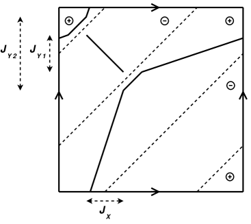
Figure 4: Schematic support of the optimal measure from the example.

Figure 5: Two different numbered limb systems which represent Figure 4.

6 Epilog

The connections of optimal transportation to geometry and curvature — sectional [62] [68], Ricci [29] [70] [71] [79] [83] [95] [104], and mean [63] — have become abundantly clear in recent years. Connections to differential topology remained largely unsuspected. The results reviewed above highlight the delicacy of identifying the extremality of a doubly stochastic measure from its support, and the role played by critical points of the transportation cost (7) in guaranteeing the uniqueness of the extremal measure $\gamma\in\Gamma(\mu,\nu)$ which solves a Kantorovich transportation problem (15) set on the ball or sphere $X$. When the sources $\mu$ are continuously distributed, the topology of the landscape $X$ limits the support of $\gamma$ to lie on a graph in the case of a ball, and a numbered limb system with two limbs in the case of a sphere. This characterization is dimension independent. For landscapes with more complicated topology, not a single example of a cost function $c\in C^{1}(X\times Y)$ is known to guarantee uniqueness of optimal measure for all continuous densities $\mu$ and $\nu$ — nor is anything known about the support of $\gamma$ beyond its numbered limb system structure and the local rectifiability determined by the rank of the cost [80] [84].

References

- [1] T. Abdellaoui and H. Heinich. Sur la distance de deux lois dans le cas vectoriel. C.R. Acad. Sci. Paris Sér. I Math. 319 (1994) 397–400.
- [2] A. Agrachev and P.W.Y. Lee. Optimal transportation under nonholomic constraints. Trans. Amer. Math. Soc. 361 (2009) 6019–6047.
- [3] N. Ahmad. The geometry of shape recognition via a Monge-Kantorovich optimal transport problem. PhD thesis, Brown University, 2004.
- [4] L. Ambrosio. Lecture notes on optimal transport problems. In Mathematical Aspects of Evolving Interfaces, volume 1812 of Lecture Notes in Mathematics, pages 1–52. Springer, Berlin, 2003.
- [5] L. Ambrosio and S. Rigot. Optimal transportation in the Heisenberg group. J. Funct. Anal. 208 (2004) 261–301.
- [6] L. Ambrosio, B. Kirchheim, and A. Pratelli. Existence of optimal transport maps for crystalline norms. Duke Math. J. 125 (2004) 207–241.
- [7] L.A. Ambrosio, N. Gigli, and G. Savaré. Gradient flows in metric spaces and in the space of probability measures. Lecture Notes in Mathematics ETH Zürich. Birkhäuser Verlag, Basel, 2005.
- [8] V. Beneš and J. Štěpán. The support of extremal probability measures with given marginals. In M.L. Puri, P. Révész and W. Wertz, editors, Mathematical Statistics and Probability Theory. Volume A: Theoretical Aspects, pages 33–41. D. Reidel Publishing Co., Dordrecht, 1987.
- [9] P. Bernard and B. Buffoni. The Monge problem for supercritical Mañé potentials on compact manifolds. Adv. Math. 207 (2006) 691–706.
- [10] P. Bernard and B. Buffoni. Optimal mass transportation and Mather theory. J. Eur. Math. Soc. (JEMS) 9 (2007) 85–121.
- [11] J. Bertrand. Existence and uniqueness of optimal maps on Alexandrov spaces. Adv. Math. 219 (2008) 838–85.
- [12] S. Bianchini and F. Cavalletti. The Monge problem for distance cost in geodesic spaces. Preprint at http://cvgmt.sns.it/papers/biacav09/Monge@problem.pdf.
- [13] G. Birkhoff. Three observations on linear algebra. Univ. Nac. Tucum n. Revista A 5 (1946) 147–151.
- [14] G. Birkhoff. Lattice Theory. Revised Edition, volume 25 of Colloquium Publications. American Mathematical Society, New York, 1948.
- [15] G. Bouchitté, G. Buttazzo, and P. Seppecher. Shape optimization solutions via Monge-Kantorovich equation. C.R. Acad. Sci. Paris Sér. I 324 (1997) 1185–1191.
- [16] G. Bouchitté, W. Gangbo and P. Seppecher. Michell trusses and lines of principal action. Math. Models Methods Appl. Sci. 18 (2008) 1571–1603.
- [17] Y. Brenier. Décomposition polaire et réarrangement monotone des champs de vecteurs. C.R. Acad. Sci. Paris Sér. I Math. 305 (1987) 805–808.
- [18] Y. Brenier. Polar factorization and monotone rearrangement of vector-valued functions. Comm. Pure Appl. Math. 44 (1991) 375–417.
- [19] L. Caffarelli. Allocation maps with general cost functions. In P. Marcellini et al, editors, Partial Differential Equations and Applications, number 177 in Lecture Notes in Pure and Appl. Math., pages 29–35. Dekker, New York, 1996.
- [20] L.A. Caffarelli. The regularity of mappings with a convex potential. J. Amer. Math. Soc. 5 (1992) 99–104.
- [21] L.A. Caffarelli. Boundary regularity of maps with convex potentials — II. Ann. of Math. (2) 144 (1996) 453–496.
- [22] L.A. Caffarelli, M. Feldman and R.J. McCann. Constructing optimal maps for Monge’s transport problem as a limit of strictly convex costs. J. Amer. Math. Soc. 15 (2002) 1–26.
- [23] L. Caravenna. An existence result for the Monge problem in with norm cost. Preprint at http://hdl.handle.net/1963/3647.
- [24] G. Carlier. A general existence result for the principal-agent problem with adverse selection. J. Math. Econom. 35 (2001) 129–150.
- [25] G. Carlier and I. Ekeland. Structure of cities. J. Global Optim. 29 (2004) 371–376.
- [26] T. Champion and L. De Pascale. The Monge problem in . Preprint at http://cvgmt.sns.it/papers/chadep09/champion-depascale.pdf.
- [27] P.-A. Chiappori, R.J. McCann, and L. Nesheim. Hedonic price equilibria, stable matching and optimal transport: equivalence, topology and uniqueness. Econom. Theory 42 (2010) 317–354.
- [28] D. Cordero-Erausquin. Sur le transport de mesures périodiques. C.R. Acad. Sci. Paris Sér. I Math. 329 (1999) 199–202.
- [29] D. Cordero-Erausquin, R.J. McCann and M. Schmuckenschläger. A Riemannian interpolation inequality à la Borell, Brascamp and Lieb. Invent. Math. 146 (2001) 219–257.
- [30] D. Cordero-Erausquin, B. Nazaret, and C. Villani. A mass-transportation approach to sharp Sobolev and Gagliardo-Nirenberg inequalities. Adv. Math. 182 (2004) 307–332.
- [31] J.A. Cuesta-Albertos and C. Matrán. Notes on the Wasserstein metric in Hilbert spaces. Ann. Probab. 17 (1989) 1264–1276.
- [32] J.A. Cuesta-Albertos and A. Tuero-Díaz. A characterization for the solution of the Monge-Kantorovich mass transference problem. Statist. Probab. Lett. 16 (1993) 147–152.
- [33] M.J.P. Cullen. A Mathematical Theory of Large Scale Atmosphere/Ocean Flows. Imperial College Press, London, 2006.
- [34] M.J.P Cullen and R.J. Purser. An extended Lagrangian model of semi-geostrophic frontogenesis. J. Atmos. Sci. 41 (1984) 1477–1497.
- [35] M.J.P Cullen and R.J. Purser. Properties of the Lagrangian semi-geostrophic equations. J. Atmos. Sci. 46 (1989) 2684–2697.
- [36] P. Delanoë. Classical solvability in dimension two of the second boundary-value problem associated with the Monge-Ampère operator. Ann. Inst. H. Poincarè Anal. Non Linèaire 8 (1991) 443–457.
- [37] J.L. Denny. The support of discrete extremal measures with given marginals. Michigan Math. J. 27 (1980) 59–64.
- [38] R. Dobrushin. Definition of a system of random variables by means of conditional distributions (Russian). Teor. Verojatnost. i Primenen. 15 (1970) 469–497.
- [39] R.D. Douglas. On extremal measures and subspace density. Michigan Math. J. 11 (1964) 243–246.
- [40] R.M. Dudley. Real Analysis and Probability. Revised reprint of the 1989 original. Cambridge University Press, Cambridge, 2002.
- [41] I. Ekeland. Existence, uniqueness and efficiency of equilibrium in hedonic markets with multidimensional types. Econom. Theory 42 (201) 275–315.
- [42] L.C. Evans and W. Gangbo. Differential equations methods for the Monge-Kantorovich mass transfer problem. Mem. Amer. Math. Soc. 137 (1999) 1–66.
- [43] A. Fathi and A. Figalli. Optimal transportation on non-compact manifolds. Israel J. Math. 175 (2010) 1–59.
- [44] M. Feldman and R.J. McCann. Monge’s transport problem on a Riemannian manifold. Trans. Amer. Math. Soc. 354 (2002) 1667–1697.
- [45] M. Feldman and R.J. McCann. Uniqueness and transport density in Monge’s transportation problem. Calc. Var. Partial Differential Equations 15 (2002) 81–113.
- [46] A. Figalli. Existence, uniqueness and regularity of optimal transport maps. SIAM J. Math. Anal. 39 (2007) 126–137.
- [47] A. Figalli. The Monge problem on non-compact manifolds. Rend. Sem. Mat. Univ. Padova, 117:147–166, 2007.
- [48] A. Figalli and N. Gigli. Local seimconvexity of Kantorovich potentials on noncompact manifolds. To appear in ESAIM Control Optim. Calc. Var.
- [49] A. Figalli, Y.-H. Kim, and R.J. McCann. When is multidimensional screening a convex program? Preprint at www.math.toronto.edu/mccann.
- [50] A. Figalli and L. Rifford. Mass transportation on sub-Riemannian manifolds. Geom. Funct. Anal. 20 (2010) 124–159.
- [51] A. Figalli, F. Maggi and A. Pratelli. A mass transportation approach to quantitative isoperimetric inequalities. To appear in Invent. Math.
- [52] W. Gangbo. Habilitation thesis. Université de Metz, 1995.
- [53] W. Gangbo and R.J. McCann. Optimal maps in Monge’s mass transport problem. C.R. Acad. Sci. Paris Sér. I Math. 321 (1995) 1653–1658.
- [54] W. Gangbo and R.J. McCann. The geometry of optimal transportation. Acta Math. 177 (1996) 113–161.
- [55] W. Gangbo and R.J. McCann. Shape recognition via Wasserstein distance. Quart. Appl. Math. 58 (2000) 705–737.
- [56] N. Gigli. On the inverse implication of Brenier-McCann theorems and the structure of . Preprint at http://cvgmt.sns.it/papers/gigc/Inverse.pdf.
- [57] T. Glimm and V. Oliker. Optical design of single reflector systems and the Monge-Kantorovich mass transfer problem. J. Math. Sci. 117 (2003) 4096–4108.
- [58] K. Hestir and S.C. Williams. Supports of doubly stochastic measures. Bernoulli 1 (1995) 217–243.
- [59] R. Jordan, D. Kinderlehrer and F. Otto. The variational formulation of the Fokker-Planck equation. SIAM J. Math. Anal. 29 (1998) 1–17.
- [60] L. Kantorovich. On the translocation of masses. C.R. (Doklady) Acad. Sci. URSS (N.S.) 37 (1942) 199–201.
- [61] L. Kantorovich. On a problem of Monge (In Russian). Uspekhi Math. Nauk. 3 (1948) 225–226.
- [62] Y.-H. Kim and R.J. McCann. Continuity, curvature, and the general covariance of optimal transportation. Preprint at www.math.toronto.edu/mccann. To appear in J. Eur. Math. Soc. (JEMS).
- [63] Y.-H. Kim, R.J. McCann and M. Warren. Pseudo-Riemannian geometry calibrates optimal transportation. Preprint at www.math.toronto.edu/mccann. To appear in Math. Res. Lett.
- [64] M. Knott and C.S. Smith. On the optimal mapping of distributions. J. Optim. Theory Appl. 43 (1984) 39–49.
- [65] T.C. Koopmans. Optimum utilization of the transportation system. Econometrica (Supplement) 17 (1949) 136–146.
- [66] V.L. Levin. Abstract cyclical monotonicity and Monge solutions for the general Monge-Kantorovich problem. Set-valued Anal. 7 (1999) 7–32.
- [67] J. Lindenstrauss. A remark on doubly stochastic measures. Amer. Math. Monthly 72 (1965) 379–382.
- [68] G. Loeper. On the regularity of solutions of optimal transportation problems. Acta Math. 202 (2009) 241–283.
- [69] V. Losert. Counterexamples to some conjectures about doubly stochastic measures. Pacific J. Math. 99 (1982) 387–397.
- [70] J. Lott. Optimal transport and Perelman’s reduced volume. Calc. Var. Partial Differential Equations 36 (2009) 49–84.
- [71] J. Lott and C. Villani. Ricci curvature for metric measure spaces via optimal transport. Annals Math. (2) 169 (2009) 903–991.
- [72] X.-N. Ma, N. Trudinger and X.-J. Wang. Regularity of potential functions of the optimal transportation problem. Arch. Rational Mech. Anal. 177 (2005) 151–183.
- [73] R.J. McCann. A Convexity Theory for Interacting Gases and Equilibrium Crystals. PhD thesis, Princeton University, 1994.
- [74] R.J. McCann. A convexity principle for interacting gases. Adv. Math. 128 (1997) 153–179.
- [75] R.J. McCann. Equilibrium shapes for planar crystals in an external field. Comm. Math. Phys. 195 (1998) 699–723.
- [76] R.J. McCann. Exact solutions to the transportation problem on the line. R. Soc. Lond. Proc. Ser. A Math. Phys. Eng. Sci., 455 (199) 1341–1380.
- [77] R.J. McCann. Polar factorization of maps on Riemannian manifolds. Geom. Funct. Anal. 11 (2001) 589–608.
- [78] R.J. McCann and M. Sosio. Hölder continuity of optimal multivalued mappings. Preprint at www.math.toronto/mccann.
- [79] R.J. McCann and P. Topping. Ricci flow, entropy, and optimal transportation. Amer. J. Math. 132 (2010) 711–730.
- [80] R.J. McCann, B. Pass and M. Warren. Rectifiability of optimal transportation plans. Preprint at www.math.toronto/mccann.
- [81] G. Monge. Mémoire sur la théorie des déblais et de remblais. Histoire de l’Académie Royale des Sciences de Paris, avec les Mémoires de Mathématique et de Physique pour la même année, pages 666–704, 1781.
- [82] F. Otto. The geometry of dissipative evolution equations: The porous medium equation. Comm. Partial Differential Equations 26 (2001) 101–174.
- [83] F. Otto and C. Villani. Generalization of an inequality by Talagrand and links with the logarithmic Sobolev inequality. J. Funct. Anal. 173 (2000) 361–400.
- [84] B. Pass. The multi-marginal optimal transportation problem. Preprint.
- [85] A.Yu. Plakhov. Exact solutions of the one-dimensional Monge-Kantorovich problem (Russian). Mat. Sb. 195 (2004) 57–74.
- [86] A.Yu. Plakhov. Newton’s problem of the body of minimal averaged resistance (Russian). Mat. Sb. 195 (2004) 105–126.
- [87] J. Purser and M.J.P. Cullen. J. Atmos. Sci 44 (1987) 3449–3468.
- [88] S.T. Rachev and L. Rüschendorf. Mass Transportation Problems. Probab. Appl. Springer-Verlag, New York, 1998.
- [89] L. Rüschendorf. Optimal solutions of multivariate coupling problems. Appl. Math. (Warsaw) 23 (1995) 325–338.
- [90] L. Rüschendorf. On -optimal random variables. Statist. Probab. Lett. 37 (1996) 267–270.
- [91] L. Rüschendorf and S.T. Rachev. A characterization of random variables with minimum -distance. J. Multivariate Anal. 32 (1990) 48–54.
- [92] T.L. Seethoff and R.C. Shiflett. Doubly stochastic measures with prescribed support. Z. Wahrscheinlichkeitstheorie und Verw. Gebiete 41 (1978) 283–288.
- [93] C. Smith and M. Knott. On the optimal transportation of distributions. J. Optim. Theory Appl. 52 (1987) 323–329.
- [94] C. Smith and M. Knott. On Hoeffding-Fréchet bounds and cyclic monotone relations. J. Multivariate Anal. 40 (1992) 328–334.
- [95] K.-T. Sturm. On the geometry of metric measure spaces, I and II. Acta Math. 196 (2006) 65–177.
- [96] V.N. Sudakov. Geometric problems in the theory of infinite-dimensional probability distributions. Proc. Steklov Inst. Math. 141 (1979) 1–178.
- [97] H. Tanaka. An inequality for a functional of probability distributions and its application to Kac’s one-dimensional model of a Maxwellian gas. Z. Wahrscheinlichkeitstheorie und Verw. Gebiete 27 (1973) 47–52.
- [98] N.S. Trudinger. Isoperimetric inequalities for quermassintegrals. Ann. Inst. H. Poincar Anal. Non Lin aire 11 (1994) 411–425.
- [99] N.S. Trudinger and X.-J. Wang. On the Monge mass transfer problem. Calc. Var. Paritial Differential Equations 13 (2001) 19–31.
- [100] N.S. Trudinger and X.-J. Wang. On the second boundary value problem for Monge-Ampère type equations and optimal transportation. Ann. Sc. Norm. Super. Pisa Cl. Sci. (5) 8 (2009) 1–32.
- [101] L. Uckelmann. Optimal couplings between onedimensional distributions. In V. Benes and J. Stepan, editors, Distributions with given marginals and moment problems, pages 261–273. Kluwer Academic Publishers, Dordrecht, 1997.
- [102] J. Urbas. On the second boundary value problem for equations of Monge-Ampère type. J. Reine Angew. Math. 487 (1997) 115–124.
- [103] C. Villani. Cours d’Intégration et Analyse de Fourier. http://www.umpa.ens-lyon.fr/ cvillani/Cours/iaf-2006.html, 2006.
- [104] C. Villani. Optimal Transport. Old and New, volume 338 of Grundlehren der Mathematischen Wissenschaften [Fundamental Principles of Mathematical Sciences]. Springer, New York, 2009.
- [105] J. von Neumann. A certain zero-sum two-person game equivalent to the optimal assignment problem. In Contributions to the theory of games. Volume 2, pages 5–12. Princeton University Press, Princeton NJ, 1953.
- [106] X.-J. Wang. On the design of a reflector antenna. Inverse Problems 12 (1996) 351–375.
- [107] X.-J. Wang. On the design of a reflector antenna II. Calc. Var. Partial Differential Equations 20 (2004) 329–341.