Toward a General Understanding of the Scaling Laws in Human and Animal Mobility

Abstract

Recent research highlighted the scaling property of human and animal mobility. An interesting issue is that the exponents of scaling law for animals and human in different situations are quite different. This paper proposes a general optimization model, a random walker following scaling laws (whose traveling distances in each step obey a power law distribution with exponent $\alpha$) tries to diversify its visiting places under a given total traveling distance with a home return probability. The results show that different optimal exponents in between $1$ and $2$ can emerge naturally. Therefore, the scaling property of human and animal mobility can be understood in our framework where the discrepancy of the scaling law exponents is due to the home return constraint under the maximization of the visiting places diversity.

The scaling laws of animal mobility indicate a class of random walks (which is also called Lévy flights), whose each step jump distance $l$ typically follows a power-law distribution of

$$P(l)\propto l^{-\alpha},$$ (1)

where $1<\alpha\leq 3$. This kind of random walks capture the property of the foraging behaviors[viswanathan_physics_2011] of albatrosses[1], terrestrial animals[2] and submarine predators[3]. On one hand, the exponents in animal foraging behaviors are always approaching $2$ (e.g. $\alpha\approx 2$ for albatross[1], deer[2], and Atlantic cod (Gadus morhua)[3], and, $\alpha\approx 1.9$ for leatherback turtle (Dermochelys coriacea), $\alpha\approx 1.7$ for Magellanic penguin (Spheniscus magellanicus)). Even for human hunters, as Brown et al. [4] pointed out, the scaling exponent is also approaching $2$ as other foraging species.

On the other hand, as recent experimental researches highlighted, the scaling laws (Eq.1) can be generalized as an approximation to the human traveling patterns[5, 6, 7, 1]. However, the exponents are much less than the ones of animal foraging behaviors, such as $\alpha\approx 1.59$ in Brockmann’s bank notes tracking study[5], $\alpha\approx 1.2$ in Gonzalez’s mobile phone users mobility[6] and $\alpha\approx 1.55$ in Song’s high resolution data[7].

It is notable that, the difference of scaling exponents is not negligible ($\Delta\alpha_{i}/\alpha_{i}\approx 25.78\%$ for individual or $\Delta\alpha_{p}/\alpha_{p}\approx 66.6\%$ for population[6]) and is mainly due to the behaviors in different situations. For the human traveling or transportation behaviors (e.g. bank notes and mobile phone users), the exponents are approaching $1$; while for the active searching (foraging) in the food lacking environments[8, 9], the exponents are around $2$.

What is the mechanism underlying the scaling behaviors with different exponents? On one hand, Visawanathan et al. have proposed a model[10] to explain the animal’s foraging behavior, in which they assumed that the forager searches for food “sites” following Eq.1 with variant exponents. They calculated the efficiency of search as the mean flights taken between two successively visited sites and obtained the optimal exponent $\alpha_{opt}=2$ which yields the best searching efficiency. Although this model can fit the foraging behaviors very well, it fails to explain human traveling behaviors ($\alpha\approx 1$).

On the other hand, some recent studies tried to explain the human traveling patterns, i.e., the scaling behaviors with exponent approaching $1$. For example, Song et al. [7] assumed that in each time step the individual may look for a new place which is never visited before or go back some visited places (e.g. home or work place). This stochastic model can explain their observed human mobility data. Han et al. [11] attributed the origin of human mobility patterns to the hierarchical structure of streets. Nevertheless, these models cannot explain the foraging behaviors.

Therefore, it still requires a general explanation. Despite the significance of the discrepancy of scaling exponents is pointed out by[12], it is still poorly understood. In this paper, we try to propose a general model of human and animal mobility.

First, we assume that one of the most important driving forces of universal mobility patterns is diversity. That is, the random walker “tries to” maximize the diversity of his visiting locations (which is measured by the Shannon entropy) within the limited total distance[13]. This constraint can be also understood as the energy constraints of human traveling behaviour[14, buldyrev_dynamical_2003, santos_optimal_2004]. Here, we should claim that the maximum diversity (entropy) is achieved not by the intentional calculations of the random walker but as a most possible result of the underlying stochastic process [13, 15, 16]. Furthermore, this assumption is consistent with Visawanathan et al. ’s model in the foraging behaviors because seeking foods with highest efficiency in the food lacking environment is equivalent to diversifying visiting places under the total distance constraints[10]. And also, diversity is a very important driving force in people’s daily lives and economic development [17, 18, 19]. This can be reflected by maximizing the diversity of visiting places in human traveling. This assumption is also coincident with exploring new places in Song’s model[7].

Second, the other important driving force exerting on the random walker is the home return constraint. In other words, the random walker must return home (a giving site) with a fixed probability in our model. This assumption is also supported by our daily experience and previous works[7]. Both animals and human beings always return some fixed points (homes, working places, schools etc.).

Under the above two important presumptions, we observe that different scaling exponents in between $1$ and $2$ can emerge naturally under different home return probability in the process of maximizing the diversity of visiting places. Therefore, our model provides a possible general understanding of human and animal mobility scaling properties.

1 The Model

Suppose the mobility space is an $L\times L$ toroidal lattice (where $L$ is a given constant denoting the world size). The random walker indicating an individual of human or animal can travel around in this lattice according to the given scaling behavior. In other words, the movement $\vec{\rho_{t}}=(x,y)$ in the $t$th time step is a two dimensional random vector whose length $|\vec{\rho_{t}}|$ following Eq. 1 with the exponent $\alpha$. The purpose of this model is not to explain the origin of scaling law but to study how the home-return tendency affects the power law exponent $\alpha$, therefore, scaling law, i.e., Eq. 1 is a basic assumption which can be supported by the previous studies[5, 6, 10].

Second, we should consider the home return constraint which is a distinct feature of our model. In reality, human or animal individual periodically visits or returns some specific places such as home or working place[7]. However, in our model, we suppose that the random walker should return to only one place called “home site” with a fixed return probability $r$. The reasons why we select only one site as home are following: 1. To keep the model as simple as possible (The multiple fixed sites cases will be studied in the future); 2. In the case of human traveling, although people always travel in between home and working place, the distance between the two points is quite small considering the whole mobility space[7, 5]. So, we can use “home site” to stand for the aggregation of these two points. Without losing generality, we suppose the “home site” is just the axis origin point $O=(0,0)$.

Thus, the integrate stochastic process can be described as follows. In time step $t$, suppose the current position of the random walker is $\vec{x_{t}}$. Then the next position in the time step $t+1$ is

$$\vec{x_{t+1}}= \vec{x_{t}}+\vec{\rho_{t}}, \vec{x_{t}}=O \theta>r$$ if or (2a)

$$\vec{x_{t+1}}= O, t=0 \vec{x_{t}}\neq O \theta\leqq r$$ if or and . (2b)

where, $\theta$ is an independent random number evenly distributed in $[0,1]$ and $\vec{\rho_{t}}$ is an independent random vector in two dimensions with a random length distributed following the scaling law (Eq. 1). So the random walker starts from the origin at $t=0$ and jumps out to other places with probability $1-r$ following Eq. 1 step by step. It may return back home with a probability $r$ in each time step.

To avoid the infinite repetition of this model, a stopping condition is added. We assume that the total distance of this random walker instead of the total number of time steps is given. That is, we have the following constraint

$$\sum_{t=1}^{T}|\vec{\rho_{t}}|\leq W=cL,$$ (3)

where $W$ is proportional to $L$ ($c$ is a given constant). It is reasonable to assume that the total distance is proportional to the total energy consumed by the random walker, so this constraint is consistent with the energy consumptions in spatial network[14, 20, buldyrev_dynamical_2003, santos_optimal_2004]. Actually, for given $W$, the total time steps $T$ is a random number. Theoretically, the distribution and expectation value of $T$ can be obtained by solving the first passage time problem, and in this way the average stopping time $T$ is dependent on $\alpha$(see the supplementary material). However, in the simulation, we just generate a set of random vectors $\vec{\rho_{t}}$ until the total distance constraint Eq. 3 is violated to get $T$.

Eq. 1, 2a and 3 actually define the dynamical process of the random walker. Under the dynamics, different sites may have different chances to be visited by the random walker in his whole life. Obviously, the sites around the home site will be visited more frequently in the tight home return constraint (i.e., large $r$). Formally, let $\{\vec{x_{1}},\vec{x_{2}},...,\vec{x_{T}}\}$ denote the sequence of sites that the random walker have visited in all steps of one realization of the random process. Then, the visited probability of each site $\vec{x}$ is defined as:

$$p(\vec{x})=\sum_{t=1}^{T}{\delta_{\vec{x_{t}}-\vec{x}}}/T,$$ (4)

where, $\delta_{\vec{y}}$ is the Kronecker’s delta function. It is $1$ only when $\vec{y}=O$, otherwise it is always $0$. We can plot visited probability of all sites in four simulations in Fig 1. This figure can be compared to the empirical distribution in [6].

Figure 1: The visited probability of each site in four different cases with $L=100,W=100000$. The visited probability distribution is comparable with the empirical results in [6] qualitatively

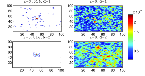
Finally, we assume that the underlying reason to form mobility scaling patterns is the driving force of maximization of the visiting places diversity. This trend can be quantified by maximizing the Shannon entropy of the visited probability. The Shannon entropy is defined as[21]:

$$S=-\sum_{\vec{x}}^{L\times L}{p(\vec{x})\log p(\vec{x})}.$$ (5)

The summation is taken for all sites.

Therefore, a complete optimization problem is defined. We will find an optimal exponent $\alpha$ to maximize Eq. 5 under the dynamical rule Eq. 2a and total distance constraint Eq. 3. Obviously, different home-return probability $r$ will systematically influence the optimal exponent $\alpha$. Next, we will show the simulation results of this model in the main text. And the analytic results in some special cases are presented in the supplementary material.

2 Results

Because our main purpose is to study how the home-return pattern affects the optimal exponent. We can first consider two extremal cases, i.e.,“never back” case ($r=0$) and “immediate back” case ($r=1$). In the first case, the trajectories of the random walker are not constraint by return probability. It means that the home site is not effective and the random walker will travel until $W$ was fully consumed. In the second case, the random walker immediately flies back home after one step walk. The optimal exponents maximizing the entropy should be quite different in the two cases. The simulation results are shown in Fig.2.

Figure 2: Entropy $S$ v.s. exponent $\alpha$ in extremal cases ($L=10000$,$W=L$ or $10L$). Each result on the figure is the ensemble average of 100 experiments. We can observe that the information entropy of visited probability will change with $\alpha$. The optimal $\alpha$ which can maximize $S$ appears in different positions with different home-return probability $r$. The optimal exponent is around $1$ when $r=1$ and $2$ when $r=0$.

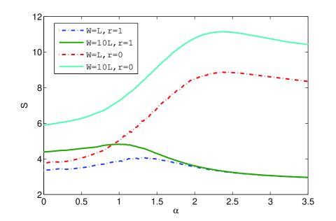
From Fig.2, we can observe that the optimal exponent $\alpha_{ib}$ in the “immediate back” case ($r=1,W=L,10L$) is around $1$. However, the optimal exponents $\alpha_{nb}$ for the “never back” case ($r=0,W=L,10L$) are from $2$ to $2.3$ with different $W$. The optimal exponent in other cases of the optimized problem should be in between of $\alpha_{ib}$ and $\alpha_{nb}$. With simulation results in the above two extremal cases alone, we have confirmed that the home return probability $r$ does have influenced the scaling law.

To approach how the home-return probability affects the scaling law, we have done another group of simulations in which the overall distance $W=10*10000$ is fixed and home return probability $r$ varies ranging from $0$ to $1$. We draw the curves showing how the exponent $\alpha$ affects the entropy $S$ for different $r$ in Fig.3 and 4.

Figure 3: The dependence of entropy $S$ on $\alpha$ in different $r$($L=10000,W=10L$). The entropy $S$ changes with $\alpha$ and get maximal values in the interval around $[1,2]$ when $r$ changes from $0$ to $1$. All curves are average results of 100 experiments

Figure 4: The dependence of entropy $S$ on $r$ and $\alpha$ ($L=10000,W=10L$). All curves are average results of 100 experiments

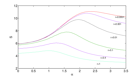
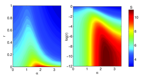
According to Fig. 3 and 4, the optimal exponent $\alpha_{opt}$ changes from around $1$ to $2$ as $r$ decreases. This result tells us that to maximize the total entropy, a random walker seldom travel long distances when it is more bound to the home site. And as we expected, the information entropy $S$ decreases when $r$ increases, since random walker’s capacity of information foraging is constraint by home-return.

Figure 5: The dependence of optimal $\alpha$ and $S$ on $r$. Where, $L=10000$,$W=L,10L$. We can observe that there is an apparent transition of the optimal $\alpha$ from $2$ to $1.5$ when $r$ is around $[10^{-3.5},0.1]$. This transition is just the key factor that distinguishes human traveling and foraging behaviors. All curves are average results of 100 experiments

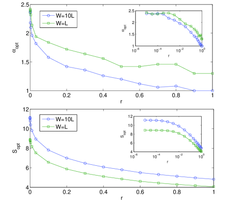
One may ask a question: how the home-return probability (i.e., $r$) affects the optimal exponent $\alpha_{opt}$? To study this issue, we conducted another group of simulations with different $r$ and plot the curve of $(r,\alpha_{opt})$ in Fig. 5. From the plot we see that the value of the optimal exponent $\alpha_{opt}$ decreases slowly at first when $r$ is in $[10^{-5},10^{-4}]$ and quickly falls down from $2$ to $1.5$ when $r$ is in $[10^{-3.4},10^{-1}]$. At last, it drops from $1.5$ to $1$ slowly when $r$ is larger than $0.1$. This result indicates that the optimal scaling exponent $\alpha_{opt}$ is determined by the home-return probability, especially when $r\in[10^{-3.4},10^{-1}]$). It is reasonable to regard the home-return probability $r=0.1$ as the critical point to distinguish foraging behaviors and traveling behaviors. The interval $(0,0.1]$ corresponds to active searching behaviors and $(0.1,1]$ is for human traveling behaviors. This critical point can be also observed in the plot of $S_{opt}$ (the corresponding entropy in the optimal exponent $\alpha$) versus $r$. Notice that the $S_{opt}$-$r$ curve has a sudden change when $r<0.1$. Furthermore, from Fig. 5 we can also observe that the optimal exponent can be distinguished much easier in different $r$ values when $W$ is big. So, our conclusion is much better for the asymptotic behavior when $W$ goes infinity.

3 Conclusion

To summarize, we propose a general framework to understand the mobility of human and animals based on the maximization of information entropy and home-return constraint. Our model reveals that the observed scaling exponents (1 for human traveling and 2 for foraging) are the results of maximizing information entropy. Second, our model points out that the home-return constraint is very important and influences the optimal exponents of mobility scaling law dramatically. The difference of scaling exponents between human traveling behaviors and foraging behaviors is due to the strength of home-return constraint.

As we know, human or animal mobility pattern is a key factor to study various related topics, such as spatial networks[22] gene pool diversity, mobile viruses and epidemic spreading. Although we have not seriously fitted the simulation to empirical data, our exploratory work contributes to mobility research by highlighting the importance of home-return pattern based on a reasonable defined model and large scale simulation. We inferred that the home-return pattern is also crucial for approaching the origin of patterns for cities, traffic systems and other related area.

4 Appendix

In the main text, we have proposed an optimal model to explain the discrepancy of the power law exponent in human or animal mobility patterns. However, we only presented the simulation results due to the complexity of the model. To understand the mathematical essence of the model and get more solid conclusions, we try to analyze this problem in a more mathematical way.

You will see, in some extreme cases, the model can be described by pure mathematical equations. Unfortunately, not all of these equations are solvable, so we have to give the numeric results instead of the exact analytic solutions. The main purpose of this analysis is trying to give a much clearer understanding toward the original problem but not a complete mathematical solution. We will discuss this problem in two extreme cases according to the home return probability $r$, namely, $r=1,r=0$.

4.1 Immediate Return ($r=1$)

According to our dynamical rules, when $r=1$ the random walker will jump out following power law distribution (Eq. 1), and return back to the home site immediately, and then, it will jump out again and fly back, and so on until the $T^{th}$ time step when its total distance is consumed up.

Because each jump-out and return back cycle is independent on the previous cycle, the final result can be converted to an equivalent problem: $T$ random walkers start to jump one step out from the home site simultaneously according to the scaling law (Eq. 1). Therefore, the original temporal experiment is converted to an ensemble experiment.

Suppose the probability of the random walker visits any site $\vec{x}=(x,y)$ is $p(\vec{x})$, and the site $\vec{x}$ is visited by $\eta(\vec{x})$ random walkers in the all $T$ walkers. Therefore, the probability that $\eta(\vec{x})=i$ is a binomial distribution,

$$P\{\eta(\vec{x})=i\}=C_{T}^{i}{(p(\vec{x}))^{i}(1-p(\vec{x}))^{T-i}},$$ (6)

Thus, the average visiting times of site $\vec{x}$ is:

$$\langle\eta(\vec{x})\rangle=Tp(\vec{x}),$$ (7)

So, the average visit frequency of site $\vec{x}$ is:

$$\mu(\vec{x})=\frac{\langle\eta(\vec{x})\rangle}{\sum_{\vec{x}}{\langle\eta(\vec{x})\rangle}}=p(\vec{x}),$$ (8)

which is independent on the total number of walkers $T$. Then, the Shannon entropy can be calculated as:

$$S=-\sum_{\vec{x}}^{L\times L}{p(\vec{x})\log p(\vec{x})},$$ (9)

which is also independent on $T$. Next, we will give the concrete mathematical form of $p(\vec{x})$ so that the relationship between $S$ and the exponent $\alpha$ will be given. We know that $p(\vec{x})$ is a Pareto power law distribution only when $\alpha>1,L\rightarrow\infty$, so, we have:
i.When $\alpha>1$,

$$p(\vec{x})=\frac{1}{Z}|\vec{x}|^{-\alpha-1}=\frac{1}{Z}(x^{2}+y^{2})^{-\frac{\alpha+1}{2}},$$ (10)

for any $|\vec{x}|\geqslant 1$,where

$$Z =\iint_{|\vec{x}|>1}{|\vec{x}|^{-\alpha-1}d\vec{x}}=\int_{0}^{2\pi}{d\theta}\int_{1}^{+\infty}{\rho^{-\alpha-1}\rho d\rho}$$ (11)

$$=\frac{2\pi}{\alpha-1}.$$

Notice that there are $2\pi|\vec{x}|$ points having the distance $|\vec{x}|$ from the origin and having the visit probability proportional to $|\vec{x}|^{-\alpha}$ , so for each point $\vec{x}$, the visit probability should be proportional to $|\vec{x}|^{-\alpha-1}$.

Thus the entropy can be approximated by an integration when $L\rightarrow\infty$:

$$S =-\iint_{|\vec{x}|>1}{p(\vec{x})\log{p(\vec{x})}d\vec{x}}$$ (12)

$$=-\int_{0}^{2\pi}{d\theta}\int_{1}^{L}{\frac{\alpha-1}{2\pi}\rho^{-\alpha-1}\log(\frac{\alpha-1}{2\pi}\rho^{-\alpha-1})\rho d\rho}$$

$$=\frac{\alpha+1+(\alpha-1)\log\frac{2\pi}{\alpha-1}}{\alpha-1},$$

and, we have,

$$\frac{\partial{S(\alpha)}}{\partial{\alpha}}=\frac{\log{\frac{2\pi}{\alpha-1}}}{\alpha-1}-\frac{\alpha+1+(\alpha-1)\log{\frac{2\pi}{\alpha-1}}}{(\alpha-1)^{2}},$$ (13)

which is always smaller than 0 when $\alpha>1$. Therefore, we can conclude that $S(\alpha)$ is a monotonic decreasing function.

ii. When $0<\alpha<1$

We know that the distribution $p(\vec{x})$ is not a standard Pareto power law distribution but have an upper bound of $|\vec{x}|$ in this case, so the entropy cannot be calculated as the previous case. We will analyze the asymptotic behavior when $L\rightarrow\infty$.

At first, we know that $p(\vec{x})$ is proportional to $|\vec{x}|^{-\alpha-1}$, therefore, Eq. 10 is still hold. However,$|\vec{x}|$ cannot go to the infinity but have an upper bound $L$. And also, $Z$ is a normalization constant, it is calculated as:

$$Z =\iint_{L>|\vec{x}|>1}{|\vec{x}|^{-\alpha-1}d\vec{x}}=\int_{0}^{2\pi}{d\theta}\int_{1}^{L}{\rho^{-\alpha-1}\rho d\rho}$$ (14)

$$=\frac{2\pi}{\alpha-1}(1-L^{1-\alpha}).$$

So, when $L\rightarrow\infty$, because $\alpha<1$, we know that:

$$p(\vec{x})=\frac{(\alpha-1)|\vec{x}|^{-\alpha-1}}{2\pi(L^{1-\alpha}-1)}\xrightarrow[]{L\rightarrow\infty}0.$$ (15)

Therefore, we know that the visit probability of each point $\vec{x}$ is approaching to $0$. That implies there are no point can be visited twice by the $T$ random walkers. In another word, we obtain an even distribution on those $T$ visited points. So the Shannon entropy can be calculated by the following formula:

$$S=-\sum_{i=1}^{T}{\frac{1}{T}\log{\frac{1}{T}}}=\log{T}$$ (16)

Instead of formula Eq.12. In this case, we can estimate the total number of walkers (or total time steps of one random walker) as follows.

We know for each “jump out and return” cycle, the average distance traveled by the walker is:

$$D =\iint_{L>|\vec{x}|>1}{|\vec{x}|\frac{1}{Z}|\vec{x}|^{-\alpha-1}d\vec{x}}$$ (17)

$$=\int_{0}^{2\pi}{d\theta}\int_{1}^{L}{\rho\frac{1}{Z}\rho^{-\alpha-1}\rho d\rho}$$

$$=\frac{\frac{2\pi}{\alpha-2}(1-L^{2-\alpha})}{\frac{2\pi}{\alpha-1}(1-L^{1-\alpha})}\approx\frac{1-\alpha}{2-\alpha}L.$$

And we know the total constraint distance can be written as,

$$W=cL,$$ (18)

where, $c$ is a constant. In the main text, we set $c=1$ or $10$ in the simulations. So, the average total number of time steps is:

$$T=\frac{W}{D}=\frac{c(2-\alpha)}{1-\alpha},$$ (19)

Bring it into Eq.16, we get:

$$S(\alpha)=\log{T}=\log{\frac{c(2-\alpha)}{1-\alpha}}.$$ (20)

And we know:

$$\frac{\partial{S(\alpha)}}{\partial{\alpha}}=\frac{1-\alpha}{(2-\alpha)c}[\frac{(\alpha-2)c}{(\alpha-1)^{2}}-\frac{c}{1-\alpha}].$$ (21)

Which is always larger than $0$ when $0<\alpha<1$. That means $S(\alpha)$ is a monotonic increasing function. So, summarizing cases i and ii, we know,

$$\frac{\partial{S(\alpha)}}{\partial{\alpha}}=\left\{\begin{aligned} &<0\ \ if\ \ \alpha>1\\ &>0\ if\ \ \alpha<1\end{aligned}\right.$$ (22)

That implies $S(\alpha)$ can get its maximal value when $\alpha=1$. Therefore, we have proved that when return probability $r=1$, the visit entropy $S$ can get its maximum when $\alpha=1$ which is consistent with our simulation result.

4.2 Never Return ($r=0$)

In this case, the random walker will keep jumping away from the home site and never come back again until its energy is consumed up.

As in the case of $r=1$, assume that in each time $t$ the visit times of a given site $\vec{x}$ is a random number $\eta(\vec{x},t)$ which follows $0-1$ distribution, that is:

$$\eta(\vec{x},t)=\left\{\begin{aligned} &1\ \ with\ probability\ \ p(\vec{x},t)\\ &0\ \ with\ probability\ \ 1-p(\vec{x},t),\end{aligned}\right.$$ (23)

where, $p(\vec{x},t)$ is the visit probability of the given site $\vec{x}$ at the $t^{th}$ time step. It can be viewed as an independent stochastic process for given $\vec{x}$. (We will get its expression latter). Then after $T$ time steps, this site $\vec{x}$ will be visited $\xi(\vec{x})$ times,

$$\xi({\vec{x}})=\sum_{t=1}^{T}{\eta(\vec{x},t)}.$$ (24)

So, its average value is:

$$\langle\xi({\vec{x}})\rangle=\sum_{t=1}^{T}{\langle\eta(\vec{x},t)\rangle}=\sum_{t=1}^{T}{p(\vec{x},t)}.$$ (25)

Then the Shannon entropy can be calculated as:

$$S =-\sum_{\vec{x}}^{L\times L}{\frac{\langle\xi(\vec{x})\rangle}{\sum_{\vec{x}}{\langle\xi(\vec{x})\rangle}}\log{\frac{\langle\xi(\vec{x})\rangle}{\sum_{\vec{x}}{\langle\xi(\vec{x})\rangle}}}}$$ (26)

$$\begin{aligned} =&-\sum_{\vec{x}}^{L\times L}{\frac{\langle\xi(\vec{x})\rangle}{\sum_{\vec{x}}{\langle\xi(\vec{x})\rangle}}\log{\langle\xi(\vec{x})\rangle}}\\ &+\sum_{\vec{x}}^{L\times L}{\frac{\langle\xi(\vec{x})\rangle}{\sum_{\vec{x}}{\langle\xi(\vec{x})\rangle}}\log{\sum_{\vec{x}}^{L\times L}{\langle\xi(\vec{x})\rangle}}}\end{aligned}$$

$$=-\sum_{\vec{x}}^{L\times L}{\frac{\langle\xi(\vec{x})\rangle}{\sum_{\vec{x}}{\langle\xi(\vec{x})\rangle}}\log{\langle\xi(\vec{x})\rangle}}+\log{\sum_{\vec{x}}^{L\times L}{\langle\xi(\vec{x})\rangle}}$$

$$\begin{aligned} =&-\sum_{\vec{x}}^{L\times L}{\{\frac{\sum_{t=0}^{T}{p(\vec{x},t)}}{\sum_{\vec{x}}{\sum_{t=0}^{T}{p(\vec{x},t)}}}\log{\sum_{t=0}^{T}{p(\vec{x},t)}}\}}\\ &+\log{\sum_{\vec{x}}^{L\times L}{\sum_{t=0}^{T}{p(\vec{x},t)}}}\end{aligned}$$

$$=-\sum_{\vec{x}}^{L\times L}{\{\frac{\sum_{t=0}^{T}{p(\vec{x},t)}}{T}\log{\sum_{t=0}^{T}{p(\vec{x},t)}}\}}+\log{T}$$

$$=-\frac{1}{T}\sum_{\vec{x}}^{L\times L}{\{\sum_{t=0}^{T}{p(\vec{x},t)}\log{\sum_{t=0}^{T}{p(\vec{x},t)}}\}}+\log{T}$$

Finally, we get a concise expression:

$$S=-\frac{1}{T}\sum_{\vec{x}}^{L\times L}{\mu(\vec{x},t)\log{\mu(\vec{x},t)}}+\log{T}$$ (27)

Where,

$$\mu(\vec{x},t)=\sum_{t=1}^{T}{p(\vec{x},t)}.$$ (28)

Therefore, the Shannon entropy is just the time average value of the entropy of the visit probability plus a constant $\log{T}$. So, $S$ is the function of $T$. However, as we know, $T$ and $p(\vec{x},t)$ are the functions of the exponent $\alpha$. Thus, we should find the expressions $T(\alpha)$ and $\mu(\vec{x},t,\alpha)$ to solve the problem. However, it is very hard to get the mathematical explicit expressions. So we will only give the numeric results instead.

i. $T(\alpha)$

For given $\alpha$ and $W$ (the total distance constraint), $T$ is a random variable. We know that in each time step, the random walker will jump out a distance $l_{t}$ which is a random number with the distance distribution $p_{l_{t}}(l)\propto l^{-\alpha}$, so according to the distance constraint, we should have the following inequality:

$$\sum_{t=1}^{T}{l_{t}}\leq W\ \ and\ \ \sum_{t=1}^{T+1}{l_{t}}>W.$$ (29)

Then, the problem becomes a classic problem of the first passage time of one-sided Lévy flight. We can convert this problem into a following equivalent one: on a one-dimensional line, a random walker starts from the origin and performs the one-sided Lévy motion (which means the random walker can only move to right but never back) until it will be attracted by a wall which locates at $W$. So the time $T$ is just the first passage time to the location $W$.

This problem has been fully discussed in the references [23, 24], and we can obtain the distribution of the random variable $T$. While, here, we only need to use the average value of $T$ as the approximation. We know that[23, 24],

$$\langle T\rangle\propto W^{\alpha-1},\ \ for\ \ 1<\alpha<2.$$ (30)

However, in our case $\alpha$ can be larger than 2. Thus, we cannot use this analytic result. Instead, we have done a large number of simulations about this one sided Lévy flight random walk and found that the power law relationship between $T$ and $W$ is always hold (see also Fig.6):

$$\langle T\rangle\propto W^{\gamma}.$$ (31)

Figure 6: The Relationship between $W$ and $T$ in different $\alpha$. The slopes ($\gamma$) of the straight lines show systematic changes

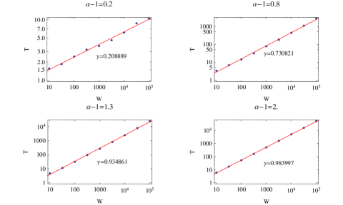
While, the exponent $\gamma$ is not always $\alpha-1$ but changes with $\alpha$ in a relationship as Fig. 7 shows.

Figure 7: The Relationship between $\gamma$ and $\alpha-1$ in the one-sided Lévy flight simulations

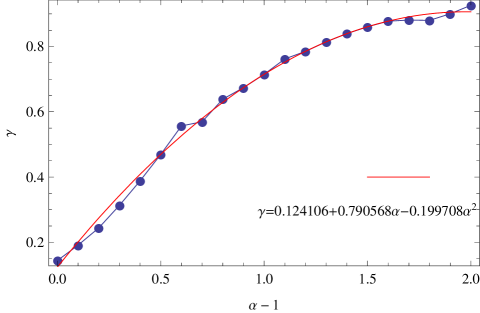
We can use a binomial equation to approach the simulation results, so we get the following relationship:

$$T(\alpha)\propto W^{0.124106+0.790568(\alpha-1)-0.199708(\alpha-1)^{2}}$$ (32)

$$for\ \ 1<\alpha<3,$$

Where, $T$ is just the traveling time under the distance constraint $W$ that we will use.

ii.$\mu(\vec{x},t)$

As we know, the time continuous Lévy flight behavior can be described by the fractional Fokker-Plank equation. That is, when $t$ is very large, $p(\vec{x},t)$ is just the approximation of the solution of the following equation[25]:

$$\frac{\partial{p(\vec{x},t)}}{\partial{t}}=\frac{\partial^{\alpha-1}p(\vec{x},t)}{\partial{x^{\alpha-1}}}.$$ (33)

Where, the right hand side has the fractional differential of the space coordinates. We can solve this equation only after the Fourier transformation, so the solution can be written as [25]:

$$p(\vec{x},t)=\frac{1}{4\pi^{2}}\iint{\exp{[i(\vec{k}\cdot\vec{x})-|\vec{k}|^{\alpha-1}t]}d\vec{k}}.$$ (34)

It is the 2-dimensional Lévy stable distribution. We know that it has no analytic solution therefore we will only give its numeric results. Finally,

$$\mu(\vec{x},t)=\frac{1}{4\pi^{2}}\sum_{t=1}^{T}{\iint{\exp{[i(\vec{k}\cdot\vec{x})-|\vec{k}|^{\alpha-1}t]}d\vec{k}}}.$$ (35)

Then, bring this result into the Eq.27, we can get the numeric result of dependency of $S$ on $\alpha$ shown in Fig. 8.

Figure 8: The relationship between $S$ and $\alpha$

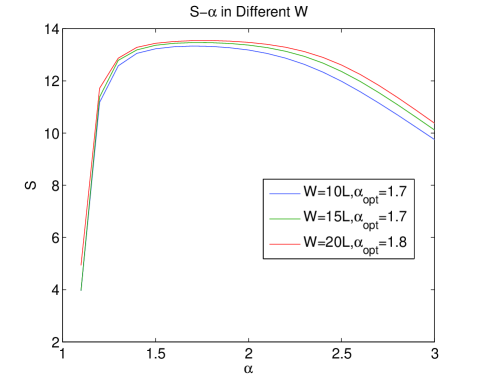
In Fig.8, we set $L=1000$, $W=10,15,20L$. We can observe that the curve can get its peak at $\alpha=1.8$ which is close to the simulation result. Although the shape of the curve is different from the simulation result (Fig.3) because lots of approximations are adopted in this analysis, their main features are similar. We can know that as the $W$ and $L$ increase, the optimal exponent will approach to the simulation result.