Effective Model Approach to the Dense State of QCD Matter

Abstract

The first-principle approach to the dense state of QCD matter, i.e. the lattice-QCD simulation at finite baryon density, is not under theoretical control for the moment. The effective model study based on QCD symmetries is a practical alternative. However the model parameters that are fixed by hadronic properties in the vacuum may have unknown dependence on the baryon chemical potential. We propose a new prescription to constrain the effective model parameters by the matching condition with the thermal Statistical Model. In the transitional region where thermal quantities blow up in the Statistical Model, deconfined quarks and gluons should smoothly take over the relevant degrees of freedom from hadrons and resonances. We use the Polyakov-loop coupled Nambu–Jona-Lasinio (PNJL) model as an effective description in the quark side and show how the matching condition is satisfied by a simple ansätz on the Polyakov loop potential. Our results favor a phase diagram with the chiral phase transition located at slightly higher temperature than deconfinement which stays close to the chemical freeze-out points.

I Introduction

Exploration of the QCD (Quantum Chromodynamics) phase diagram, particularly toward a higher baryon-density regime, is of increasing importance in both theoretical and experimental sides Fukushima:2010bq . From the theoretical point of view, so far, only the lattice-QCD simulation Fukushima:2010bq ; DeTar:2009ef ; Borsanyi:2010cj ; Bazavov:2010sb is the first-principle calculation of QCD at work to explore the phase transitions associated with chiral restoration and quark deconfinement. The Polyakov loop $\Phi$ and the chiral condensate $\langle\bar{\psi}\psi\rangle$ are the (approximate) order parameters for quark deconfinement and chiral restoration, respectively, which are gauge invariant and measurable on the lattice (though both require renormalization corrections). The lattice-QCD simulation is, however, of limited practical use and it works only when the baryon chemical potential $\mu_{\text{B}}$ is sufficiently smaller than the temperature $T$. For $\mu_{\text{B}}/T\gtrsim 1$ the notorious sign problem prevents us from extracting any reliable information from the lattice-QCD data Fukushima:2010bq ; Muroya:2003qs .

The effective model study is an alternative and pragmatic approach toward the phase diagram of dense QCD.  Some may complain that the model study relies on not QCD directly but on just a model. Results from the model analysis are, nevertheless, what we can get at best for the moment. Even within the framework of the model study there are several different attitudes. One way for theorists to go is simplify QCD so that it can be solvable without introducing further approximations. QCD-like models in lower dimensions (such as the ’t Hooft model) Schon:2000qy , the strong-coupling expansion in the lattice formulation Fukushima:2003vi , and the large-$N_{\text{c}}$ limit of QCD McLerran:2007qj are typical examples in this direction.

Here, we shall take another way to proceed into the phase structure. The idea is the following (as schematically illustrated in Fig. 1);

1. Construct a model that works for infinitely heavy quarks ($m_{q}\to\infty$) in such a way that the model respects the global symmetry (center symmetry) in the finite-$T$ pure gluonic sector.

2. Choose a chiral model based on the global symmetry (chiral symmetry) for massless quarks ($m_{q}\to 0$) in such a way that the spontaneous breakdown of chiral symmetry is correctly described.

3. Interpolate a finite-$m_{q}$ model between above-mentioned two. It is minimally required that the infinite $m_{q}$ limit and the vanishing $m_{q}$ limit should recover the above models respectively.

4. Check if the interpolation is properly chosen or not by comparing the model outputs to available lattice-QCD and/or phenomenological data.

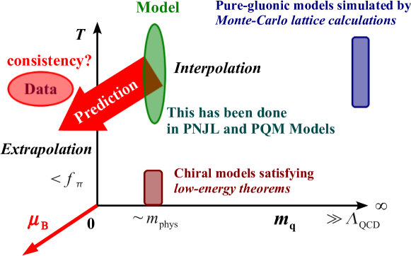
Figure 1: Schematic picture to show how the effective model is constructed as an interpolation between the pure-gluonic theory (at $m_{q}\ll\Lambda_{\text{QCD}}$ and $T\sim\Lambda_{\text{QCD}}$) and the chiral models (at $m_{q}\lesssim m_{\text{phys}}$ and $T<f_{\pi}$). The prediction from the interpolated effective model is done as an extrapolation toward some new axis such as the baryon chemical potential, whose consistency with available data must be eventually checked.

Along this line the model is not necessarily solvable and usually needs some additional approximations. Nevertheless, if the item $4$ above is taken into account very carefully, one may claim that one is dealing with a phase diagram of QCD, not of QCD-like models, in a sense that the situation one is handling is not $(1+1)$ dimensions, not $g^{2}\to\infty$, and not $N_{\text{c}}\to\infty$. Sometimes, to this aim toward the QCD phase diagram, one has to face “dirty” businesses; it is often the case that the phase structure might be significantly changed by uncontrollable model parameters, which one can take in twofold ways — pessimists would be disappointed and say that the model cannot predict anything, and on the other hand, optimists would be delighted and say that the model has clarified a non-trivial role played by the model parameter in understanding the phase diagram.

Let us briefly explain how to implement the items $1$ and $2$. In the absence of particles transforming in the color fundamental representation, the genuine gauge symmetry possessed by the pure gluonic theory is $\mathrm{SU}(N_{\text{c}})/\mathrm{Z}(N_{\text{c}})$. If one performs the $\mathrm{Z}(N_{\text{c}})$ transformation on the gauge links, the fields are shifted typically by $2\pi/(N_{\text{c}}a)$ where $a$ is a characteristic scale (lattice spacing). The perturbation theory breaks this $\mathrm{Z}(N_{\text{c}})$ symmetry but this is practically no problem because the shift goes infinity as $a\to 0$. Furthermore one can generalize the similar procedure onto not the individual gauge link but a product of the $N_{\tau}$ gauge links along a finite extent. Then, the fields are shifted by $2\pi/(N_{\text{c}}N_{\tau}a)=2\pi T/N_{\text{c}}$, which remains sensible in the $a\to 0$ limit. In this way the Polyakov loop matrix $L$ is defined, that is, $L=\prod_{\tau}U_{\tau}$ and the $\mathrm{Z}(N_{\text{c}})$ symmetry with respect to $L$ is called “center symmetry” which breaks in the perturbation theory Svetitsky:1985ye .

The expectation value of the traced Polyakov loop, $\Phi=\langle\text{tr}L\rangle$, is the order parameter for the quark deconfinement phase transition in the pure gluonic system. The most intuitive way to understand this comes from the property that $\Phi$ is related to the free energy gain of a static single quark placed in a hot gluonic medium as $\Phi=\exp[-f_{q}/T]$. Therefore $\Phi=0$ implies $f_{q}=\infty$, meaning that quarks never show up (confinement). Once $\Phi$ becomes non-vanishing, $f_{q}$ should take a finite value and thermal quark excitations are permitted. The effective action for $L$ or $\Phi$ has been computed perturbatively Gross:1980br but in order to discuss the phase transition from center symmetric to center broken phases, one needs a non-perturbative evaluation of the effective action.

Concerning the chiral dynamics, the model choice could be anything as long as it can correctly describe the dynamical chiral symmetry breaking pattern. Then, the chiral properties are almost automatically derived from the so-called low-energy (soft-pion) theorems. Of course some details of the phase transition such as the critical temperature and the thermodynamic quantities depend on the choice of the chiral model. Because we are interested in the phase transition associated with restoration of chiral symmetry, the non-linear representation is inappropriate which is based on the symmetry breaking.

The order parameter for the chiral phase transition is given by the chiral condensate $\langle\bar{\psi}\psi\rangle$. This is simple to understand — the quark mass $m_{q}$ and an operator $\bar{\psi}\psi$ are conjugate to each other, so $m_{q}$ is a source to generate $\langle\bar{\psi}\psi\rangle$ and in turn $\langle\bar{\psi}\psi\rangle$ is a source to generate the dynamical mass that breaks chiral symmetry. There are well-established chiral models such as the Nambu–Jona-Lasinio (NJL) model and the quark-meson (QM) model.

The interpolation at the item $3$ is the main problem. There is no theoretical justification at all for the existence of reasonable interpolation. We can judge how good or how bad it is only through the comparison at the item $4$. At this point it is already obvious that the Polyakov loop model is not sufficient to access the realistic QCD phase transition, though it may capture interesting phenomenological consequences Dumitru:2000in . In a similar sense conventional chiral models are not good enough to draw the QCD phase diagram even though they are usually designed to be a good description of hadronic properties in the vacuum Hatsuda:1994pi . To address the QCD phase transitions the first test for the validity of the model description should be the consistency check with the known properties available from the lattice-QCD simulation at $T\neq 0$ and $\mu_{\text{B}}=0$; the finite-$T$ behavior of two order parameters, $\Phi$ and $\langle\bar{\psi}\psi\rangle$, and the thermodynamic quantities such as the pressure, the internal energy density, the entropy density, etc.

Along this line the Polyakov-loop coupled chiral models such as the PNJL (Polyakov–NJL) Fukushima:2003fw ; Ratti:2005jh and the PQM (Polyakov-QM) Schaefer:2007pw ; Schaefer:2009ui models are quite successful to treat both order parameters on the equal footing. Besides, the Polyakov loop potential $\mathcal{U}[\Phi]$ is determined by the lattice data in the pure gluonic theory, namely, by the Polyakov loop $\Phi(T)$ and the pressure $p(T)$ as functions of $T$. This means that the PNJL and PQM models include the pressure contribution from gluons as well as quarks, so that the models are able to deal with the full thermodynamics which are to be compared with the full lattice-QCD simulation. The important point is that the dynamics of transverse gluons $A_{i}^{T}$ is also under the control of the deconfinement order parameter $\Phi$ and thus is to be encompassed in the parametrization of the Polyakov loop potential $\mathcal{U}[\Phi]$, while the Polyakov loop itself is expressed in terms of the longitudinal gluon $A_{4}$.

Here we would like to emphasize that the success of the PNJL and PQM models is far beyond the fitting physics. Model parameters are fixed separately in two regions, i.e. in the pure-gluonic theory (at $m_{q}\ll\Lambda_{\text{QCD}}$ and $T\sim\Lambda_{\text{QCD}}$) and in the chiral models (at $m_{q}\lesssim m_{\text{phys}}$ and $T<f_{\pi}$). The interpolation procedure does not involve any further fitting. It is a highly non-trivial discovery that there exists a reasonable way to make an interpolation fairly consistent with the full lattice-QCD data.

The next step one should think of is the prediction from the model. This is done by an extrapolation of the model toward some new axis such as the baryon chemical potential. By now there are different versions of the “QCD phase diagram” drawn in this way by means of the PNJL and PQM models with different parameter tunings Fukushima:2003fw ; Ratti:2005jh ; Schaefer:2007pw ; Schaefer:2009ui ; Sasaki:2006ww . If we go into small details, there are many places where we can talk about the difference. Here we shall limit ourselves to look at the difference mainly in the behavior of the Polyakov loop or the deconfinement (crossover) transition line. Some of the model results may be close to the true answer, and some may not. We must have a guiding principle to select out which is preferred and which is not. The available and reliable data at finite baryon density is, however, extremely limited. In what follows we shall elucidate the idea and find that the naive extrapolation from the PNJL and PQM models is not acceptable. To see this, we will explain the results from the thermal Statistical Model in the next section.

II Thermodynamics from the Statistical Model

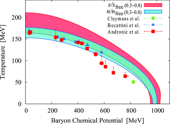
Figure 2: Chemical freeze-out points taken from Refs. Cleymans:2005xv ; Becattini:2005xt . The red and blue (upper and lower) bands represent the regions where the entropy density $s$ and the baryon number density $n$, respectively, increase quickly from $0.3$ to $0.8$ in the unit of free quark-gluon values, $s_{\text{free}}$ and $n_{\text{free}}$ (see Eq. (1)).

Regarding the QCD phase diagram at finite $T$ and $\mu_{\text{B}}$ useful information is quite limited. The lattice-QCD at finite density is being improved, but still different techniques to circumvent the sign problem lead to different results. Only the chemical freeze-out points in the heavy-ion collisions are experimental hints about the phase diagram. Although the freeze-out points shape an intriguing curve on the $\mu_{\text{B}}$-$T$ plane, as plotted by error-bar dots in Fig. 2, one should carefully interpret it.

The freeze-out points are not the raw experimental data but an interpretation through the thermal Statistical Model Cleymans:2005xv ; Becattini:2005xt . In this model the grand canonical partition function is given by contributions from the non-interacting gas of hadrons and resonances. In view of the fact that the Statistical Model is such successful to fit various particle ratios with $\mu_{\text{B}}$ and $T$ only ($\mu_{Q}$, $\mu_{\text{s}}$, and $\mu_{\text{c}}$ are determined by the collision condition), it should be legitimate to take the freeze-out points for experimental data, which in turn validates the Statistical Model (though why it works lacks for an explanation from QCD).

Let us proceed by further accepting that the Statistical Model is a valid description of the state of matter until the freeze-out curve or even slightly above. It is then a straightforward application of the Statistical Model to estimate thermodynamic quantities such as the pressure $p$, the entropy density $s$, the baryon number density $n$, etc. We here utilize the open code THERMUS ver.2.1 to calculate $s$ and $n$ at various $T$ and $\mu_{\text{B}}$ Wheaton:2004qb . From now on the Statistical Model analysis specifically means the use of THERMUS.

Figure 2 shows the chemical freeze-out points taken from Refs. Cleymans:2005xv ; Becattini:2005xt , on which $s$ and $n$ are overlaid. For convenience we normalized these quantities by

$$\begin{split}s_{\text{free}}&=\biggl{\{}(N_{\text{c}}^{2}-1)+\frac{7}{4}N_{\text{c}}N_{\text{f}}\biggr{\}}\frac{4\pi^{2}}{45}T^{3}+\frac{N_{\text{c}}N_{\text{f}}}{3}\mu_{\text{q}}^{2}T\;,\\ n_{\text{free}}&=N_{\text{f}}\biggl{(}\frac{\mu_{\text{q}}^{3}}{3\pi^{2}}+\frac{\mu_{\text{q}}T^{2}}{3}\biggr{)}\;.\end{split}$$ (1)

These are the entropy density and the baryon number density of free massless $N_{\text{c}}^{2}-1$ gluons and $N_{\text{c}}N_{\text{f}}$ quarks.

Here we note that, in drawing Fig. 2, we have intentionally relaxed the neutrality conditions for electric charge and heavy flavors and simply set $\mu_{Q}=\mu_{\text{s}}=\mu_{\text{c}}=0$. We have done so in order to make it possible to compare the results from the Statistical Model to the chiral effective model in later discussions. [We note that one can force the chiral model to satisfy neutrality but it would be technically involved Fukushima:2009dx .] Nevertheless, we would emphasize that the neutrality conditions have only minor effects on the bulk thermodynamics and make only small differences in any case. We should also mention that we used Eq. (1) with $N_{\text{c}}=N_{\text{f}}=3$. The choice of $s_{\text{free}}$ and $n_{\text{free}}$ (and relevant $N_{\text{f}}$) is arbitrary and the following discussions do not rely on this particular choice, for we will use $s_{\text{free}}$ and $n_{\text{free}}$ just as common denominators to display the Statistical Model results and the PNJL model results.

The Statistical Model cannot tell us about the QCD phase transitions. Still, Fig. 2 is already suggestive enough. We can clearly see the thermodynamic quantities from the Statistical Model blowing up in a relatively narrow region. The red and blue (upper and lower) bands indicate the regions where $s/s_{\text{free}}$ and $n/n_{\text{free}}$, respectively, grow quickly from $0.3$ to $0.8$. In the Hagedorn’s picture Cabibbo:1975ig this rapid and simultaneous rise in $s$ and $n$ has a natural interpretation as the Hagedorn limiting temperature above which color degrees of freedom is liberated, i.e. color deconfinement.

The idea here is to make use of the thermodynamics from the Statistical Model as shown in Fig. 2 to judge if the Polyakov-loop coupled chiral models work fine at finite density. We also make an important remark that this idea can be effective only up to about $\mu_{\text{B}}\lesssim 400\sim 600\;\text{MeV}$ because the chemical freeze-out points start dropping down steeply in this density region, which suggests an onset of some new form of matter; an example of such possibilities is quarkyonic matter Andronic:2009gj .

III Thermodynamics from the PNJL Model

Figure 2 is useful to make a guesstimate about the deconfinement boundary but we can deduce no information about the chiral property. This is because the thermal Statistical Model needs no medium modification driven by chiral restoration. So, to address the QCD phase transitions and associated boundaries, we must find a way to connect the thermodynamics in Fig. 2 to the order parameters $\Phi$ and $\langle\bar{\psi}\psi\rangle$. Here let us go into details of the chiral effective model.

It is crucial to adopt the Polyakov-loop coupled model here because the entropy density should contain contributions from gluons which are taken care of by the Polyakov loop potential $\mathcal{U}[\Phi]$. The PNJL model that we use below is defined with the following potential;

$$\mathcal{U}[\Phi,\bar{\Phi}]=T^{4}\biggl{\{}-\frac{a(T)}{2}\bar{\Phi}\Phi+b(T)\ln\Bigl{[}1-6\bar{\Phi}\Phi+4(\bar{\Phi}^{3}+\Phi^{3})-3(\bar{\Phi}\Phi)^{2}\Bigr{]}\biggr{\}}$$ (2)

with $a(T)=a_{0}+a_{1}(T_{0}/T)+a_{2}(T_{0}/T)^{2}$ and $b(T)=b_{3}(T_{0}/T)^{3}$. There are thus five parameters one out of which is constrained by the Stefan-Boltzmann limit, i.e. $\mathcal{U}\to-(8\pi^{2}/45)T^{4}$ at $\Phi=\bar{\Phi}=1$ in the $T\to\infty$ limit. These parameters are fixed by the pure-gluonic lattice data as $a_{0}=3.51$, $a_{1}=-2.47$, $a_{2}=15.2$, $b_{3}=-1.75$ Ratti:2005jh , and $T_{0}=270\;\text{MeV}$ from the deconfinement temperature of first order in the pure-gluonic theory Boyd:1996bx . It is important to note that only $T_{0}$ is a dimensional parameter, so that the energy scale is set by this $T_{0}$ alone.

In addition the NJL sector of the PNJL model has five more parameters in the three-flavor case Fukushima:2003fw appearing in the mean-field thermodynamic potential;

$$\begin{split}\Omega_{\text{NJL}}&=g_{S}\bigl{(}\langle\bar{u}u\rangle^{2}+\langle\bar{d}d\rangle^{2}+\langle\bar{s}s\rangle^{2}\bigr{)}+4g_{D}\langle\bar{u}u\rangle\langle\bar{d}d\rangle\langle\bar{s}s\rangle-2N_{\text{c}}\sum_{i}\int^{\Lambda}\!\frac{d^{3}p}{(2\pi)^{3}}\>\varepsilon_{i}(p)\\ &\quad-2T\sum_{i}\int\frac{d^{3}p}{(2\pi)^{3}}\biggl{\{}\ln\det\biggl{[}1+L\,e^{-(\varepsilon_{i}(p)-\mu_{\text{q}})/T}\biggr{]}+\ln\det\biggl{[}1+L^{\dagger}\,e^{-(\varepsilon_{i}(p)+\mu_{\text{q}})/T}\biggr{]}\biggr{\}}\;,\end{split}$$ (3)

where the energy dispersion relation $\varepsilon_{i}(p)$ depends on the flavor index $i$ as $\varepsilon_{i}(p)^{2}=p^{2}+M_{i}^{2}$ and the constituent quark masses are $M_{u}=m_{u}-2g_{S}\langle\bar{u}u\rangle-2g_{D}\langle\bar{d}d\rangle\langle\bar{s}s\rangle$ and so on. The model parameters are then the light and heavy quark masses $m_{\rm ud}$ and $m_{\rm s}$, the momentum cutoff $\Lambda$, the four-fermionic interaction strength $g_{S}$, and the $\mathrm{U(1)_{A}}$-breaking six-fermionic interaction strength $g_{D}$, which are all fixed by the pion mass $m_{\pi}$, the kaon mass $m_{K}$, the eta-prime mass $m_{\eta^{\prime}}$, the pion decay constant $f_{\pi}$, and the chiral condensate $\langle\bar{\psi}\psi\rangle$ Hatsuda:1994pi .

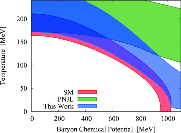
Figure 3: Entropy density normalized by $s_{\text{free}}$ (from $0.3$ to $0.8$) in the Statistical Model (bottom band with red color; same as shown in Fig. 2) and that in the PNJL model with a choice $T_{0}=200\;\text{MeV}$ (top band with green color). The blue band between two represents the results with the ansätz (5).

In the presence of dynamical quarks, if we keep using the pure-gluonic critical temperature $T_{0}=270\;\text{MeV}$, the simultaneous crossover temperature of deconfinement and chiral restoration becomes over $200\;\text{MeV}$, which is too high as compared to the lattice-QCD value. It is nicely argued in Ref. Schaefer:2007pw that the back-reaction from quark loops affects the mass scale $T_{0}$ which changes from $T_{0}=270\;\text{MeV}$ for $N_{\text{f}}=0$ down to $T_{0}=208\;\text{MeV}$ for $N_{\text{f}}=2$ and $T_{0}=187\;\text{MeV}$ for $N_{\text{f}}=2+1$ Schaefer:2007pw . Here we choose to use $T_{0}=200\;\text{MeV}$ for calculations at $\mu_{\text{B}}=0$ throughout.

In Fig. 3 we show the entropy density calculated in the mean-field PNJL model with $T_{0}=200\;\text{MeV}$ fixed, in the same way as in the Statistical Model drawn in Fig. 2. The bottom (top) band in red (green) color is the result from the Statistical Model (PNJL model). From the figure it is obvious that the PNJL model is not consistent with the Statistical Model even at the qualitative level. With the properly scaled $T_{0}$ from $270\;\text{MeV}$ down to $200\;\text{MeV}$, the blow-up behavior in $s$ from the Statistical Model can be smoothly connected to the PNJL model description only in the region up to $\mu_{\text{B}}\lesssim 400\;\text{MeV}$. The curvature of the band as a function of $\mu_{\text{B}}$ is significantly different; the PNJL model result is too flat horizontally and the green band eventually takes apart from the red region where the Statistical Model breaks down.

IV Matching Prescription

Such a manifest discrepancy from the Statistical Model is a critical drawback of the PNJL model. The situation is not changed even in the PQM model as long as $T_{0}$ is a constant. To make the entropy density at $\mu_{\text{B}}\gtrsim 400\;\text{MeV}$ get saturated earlier as is the case in the Statistical Model, quark degrees of freedom must be released at smaller temperature than predicted by the PNJL model.

One can imagine how this drawback occurs in the PNJL model study; the energy scale in the Polyakov loop potential is specified by the dimensional parameter $T_{0}$ that may differ depending on the effects of $T$ and $\mu_{\text{B}}$ in the quark sector. We have shifted $T_{0}$ from $270\;\text{MeV}$ down to $200\;\text{MeV}$, through which we have incorporated the scale change induced by $N_{\text{f}}$ quarks at finite $T$. In this way we may well consider that $T_{0}$ should decrease with increasing $\mu_{\text{B}}$ as pointed out in Ref. Schaefer:2007pw .

Our idea proposed here is to make use of Fig. 3 to fix $T_{0}(\mu_{\text{B}})$ for consistency with phenomenology. One can pick up other thermodynamic quantities than the entropy density like the internal energy density, which would anyway make little change in the final result. Besides, the choice of the entropy density is most natural because it counts the effective degrees of freedom and thus is a sensitive quantity to probe deconfinement. In Ref. Cleymans:2005xv the freeze-out curve is parametrized as

$$T_{\rm f}(\mu_{\text{B}})=a-b\,\mu_{\text{B}}^{2}-c\,\mu_{\text{B}}^{4}$$ (4)

with the fitting result $a=166(2)\;\text{MeV}$, $b=1.39(16)\times 10^{-4}\;\text{MeV}^{-1}$, and $c=5.3(21)\times 10^{-11}\;\text{MeV}^{-3}$. Because the behavior of the entropy density must be dominantly controlled by deconfinement, we postulate that the change in $T_{0}$ is to be correlated with $T_{\rm f}(\mu_{\text{B}})$. We see that the freeze-out points and the entropy band in Fig. 2 have roughly same curvature indeed. Let us simply use same $b$ and make an ansätz as

$$\frac{T_{0}(\mu_{\text{B}})}{T_{0}}=1-(bT_{0})\biggl{(}\frac{\mu_{\text{B}}}{T_{0}}\biggr{)}^{2}=1-2.78\times 10^{-2}\biggl{(}\frac{\mu_{\text{B}}}{T_{0}}\biggr{)}^{2}\;,$$ (5)

which yields the blue band in the middle of Fig. 3. [To prevent unphysical negative $T_{0}$ for large $\mu_{\text{B}}$ we set a threshold at $10\;\text{MeV}$ so that $T_{0}\geq 10\;\text{MeV}$. Hence, the results at $T<10\;\text{MeV}$ are not meaningful.] We see at a glance that the results from this modified PNJL model have a reasonable overlap with the Statistical Model results in the whole density region as plotted.

At this point one might have thought of several questions. First, the ansätz (5) might look ad hoc, but we point out that our choice happens to be very close to the independent argument in Ref. Schaefer:2007pw , in which the $\mu_{\text{B}}$-dependence has been estimated from the running coupling constant as $T_{0}(\mu_{\text{B}})=T_{\tau}e^{-1/(\alpha_{0}b(\mu_{\text{B}}))}$ which is expanded to be $T_{0}(\mu_{\text{B}})/T_{0}\simeq 1-2.1\times 10^{-2}(\mu_{\text{B}}/T_{0})^{2}+\cdots$. In the perturbative manner one can also understand how the $\mu_{\text{B}}$-dependence enters the Polyakov loop potential which consists of the closed loop of dressed gluon propagator. The quark–anti-quark polarization diagrams inserted in the gluon propagator generate the back-reaction dependent on $\mu_{\text{B}}$. There is another phenomenological ansätz for the $\mu_{\text{B}}$-dependent $\mathcal{U}[\Phi]$ Dexheimer:2009hi . Second, one might wonder if the energy scale in the quark (NJL) sector should be modified as well. Such modification is not necessary, however. This is because, as we have mentioned, the Statistical Model requires no modification associated with the chiral dynamics, which strongly implies that we do not have to introduce $\mu_{\text{B}}$ dependent changes in the NJL parameters. Third, the ansätz (5) has terms only up to the quadratic order. This means that we cannot go to high-density regions with $\mu_{\text{B}}\ll T_{0}$. This is indeed so and we have actually truncated higher-order terms in Eq. (5). In any case, as we have noted before, the idea of the entropy matching holds only up to $\mu_{\text{B}}\lesssim 400\sim 600\;\text{MeV}$, and we should not take the results in the high-density region seriously.

V Phase Diagram

Now we get ready to proceed to the possible QCD phase diagram that is fully consistent with the Statistical Model thermodynamics in Fig. 2. Using the standard computational procedure of the mean-field PNJL model we can solve $\Phi$ and $\langle\bar{\psi}\psi\rangle$ as functions of $T$ and $\mu_{\text{B}}$, from which the phase boundaries of deconfinement and chiral restoration are located.

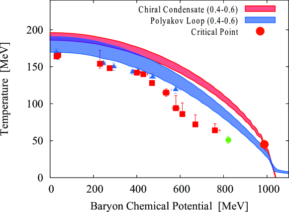
Figure 4: A figure taken from Ref. Fukushima:2010is . Phase boundaries associated with deconfinement (blue band) and chiral restoration (red band). Each band represents a region where the (normalized) order parameter develops from $0.4$ to $0.6$.

Figure 4 (the central result of Ref. Fukushima:2010is ) shows the phase diagram from the modified PNJL model. The blue (red) band is a region where the Polyakov loop (normalized light-quark chiral condensate) increases from $0.4$ to $0.6$. In contrast to the old PNJL model, the new results indicate that the chiral phase transition is almost parallel to and entirely above the deconfinement, which agrees with the situation considered phenomenologically in Ref. Castorina:2010gy . We have found the critical point Asakawa:1989bq ; Stephanov:1998dy at $(\mu_{\text{B}},T)\simeq(45\;\text{MeV},330\;\text{MeV})$, but should not take it seriously since its location is beyond the validity region of the current prescription.

VI Conclusions

It is an intriguing observation that the chiral phase transition occurs later than deconfinement. This is quite consistent with the Statistical Model assumption. In the Statistical Model the hadron masses are just the vacuum values and any hadron mass/width modifications are not considered, which would be a reasonable treatment only if the chiral phase transition is separated above the Hagedorn temperature. Under such a phase structure, besides, our assumption of neglecting $\mu_{\text{B}}$-dependence in the NJL-model parameters turns out to be acceptable in a similar sense as the Statistical Model treatment. This can be understood from the fact that the NJL part yields the hadron masses in the vacuum which are intact in the Statistical Model.

The failure of the standard PNJL model is attributed to baryonic degrees of freedom which is missing; the singlet-part of the thermal excitation in the PNJL model can be translated into an expression in terms of baryons as

$$\int\frac{d^{3}k}{(2\pi)^{3}}\;e^{-N_{\text{c}}(\sqrt{k^{2}+M_{q}^{2}}-\mu_{\text{q}})/T}=\frac{1}{N_{\text{c}}^{3}}\int\frac{d^{3}k^{\prime}}{(2\pi)^{3}}\;e^{-(\sqrt{{k^{\prime}}^{2}+M_{N}^{2}}-\mu_{\text{B}})/T}\;,$$ (6)

where $M_{N}=N_{\text{c}}M_{q}$, $\mu_{\text{B}}=N_{\text{c}}\mu_{\text{q}}$, and $k^{\prime}=N_{\text{c}}k$ with which a factor $1/N_{\text{c}}^{3}$ appears from the integration measure. Therefore, the PNJL model significantly underestimates the baryonic excitations by $1/N_{\text{c}}^{3}$. Hence, one may say that a modification made in $\mathcal{U}[\Phi]$ by hand stems, in principle, from confinement effects, which can be presumably parametrized by the Polyakov loop. This idea is reminiscent of the treatment of transverse gluons. It is an important question how our phenomenological input (5) is validated/invalidated from the first-principle QCD calculation. This may be answered by future developments in the functional renormalization group method Braun:2009gm .

References

- (1) For a recent review on the QCD phase diagram, see; K. Fukushima and T. Hatsuda, “The phase diagram of dense QCD,” arXiv:1005.4814 [hep-ph].
- (2) C. DeTar and U. M. Heller, “QCD thermodynamics from the lattice,” Eur. Phys. J. A 41, 405 (2009).
- (3) S. Borsanyi et al., “The QCD equation of state with dynamical quarks,” arXiv:1007.2580 [hep-lat].
- (4) A. Bazavov and P. Petreczky [HotQCD collaboration], “Deconfinement and chiral transition with the highly improved staggered quark (HISQ) action,” J. Phys. Conf. Ser. 230, 012014 (2010).
- (5) For a review on the sign problem, see; S. Muroya, A. Nakamura, C. Nonaka and T. Takaishi, “Lattice QCD at finite density: An introductory review,” Prog. Theor. Phys. 110, 615 (2003).
- (6) V. Schon and M. Thies, “2D model field theories at finite temperature and density,” arXiv:hep-th/0008175.
- (7) K. Fukushima, “Toward understanding the lattice QCD results from the strong coupling analysis,” Prog. Theor. Phys. Suppl. 153, 204 (2004).
- (8) L. McLerran and R. D. Pisarski, “Phases of cold, dense quarks at large ,” Nucl. Phys. A 796, 83 (2007).
- (9) For a review, see; B. Svetitsky, “Symmetry aspects of finite temperature confinement transitions,” Phys. Rept. 132, 1 (1986), and references therein.
- (10) D. J. Gross, R. D. Pisarski and L. G. Yaffe, Rev. Mod. Phys. 53, 43 (1981).
- (11) A. Dumitru and R. D. Pisarski, “Event-by-event fluctuations from decay of a condensate for Z(3) Wilson lines,” Phys. Lett. B 504, 282 (2001).
- (12) T. Hatsuda and T. Kunihiro, “QCD phenomenology based on a chiral effective Lagrangian,” Phys. Rept. 247, 221 (1994).
- (13) K. Fukushima, “Chiral effective model with the Polyakov loop,” Phys. Lett. B 591, 277 (2004); “Phase diagrams in the three-flavor Nambu–Jona-Lasinio model with the Polyakov loop,” Phys. Rev. D 77, 114028 (2008).
- (14) C. Ratti, M. A. Thaler and W. Weise, “Phases of QCD: Lattice thermodynamics and a field theoretical model,” Phys. Rev. D 73, 014019 (2006); S. Roessner, C. Ratti and W. Weise, “Polyakov loop, diquarks and the two-flavour phase diagram,” Phys. Rev. D 75, 034007 (2007).
- (15) B. J. Schaefer, J. M. Pawlowski and J. Wambach, “The Phase Structure of the Polyakov–Quark-Meson Model,” Phys. Rev. D 76, 074023 (2007) [arXiv:0704.3234 [hep-ph]].
- (16) B. J. Schaefer, M. Wagner and J. Wambach, “Thermodynamics of (2+1)-flavor QCD: Confronting Models with Lattice Studies,” Phys. Rev. D 81, 074013 (2010) [arXiv:0910.5628 [hep-ph]].
- (17) C. Sasaki, B. Friman and K. Redlich, “Susceptibilities and the phase structure of a chiral model with Polyakov loops,” Phys. Rev. D 75, 074013 (2007); L. McLerran, K. Redlich and C. Sasaki, “Quarkyonic Matter and Chiral Symmetry Breaking,” Nucl. Phys. A 824, 86 (2009).
- (18) J. Cleymans, H. Oeschler, K. Redlich and S. Wheaton, “Comparison of chemical freeze-out criteria in heavy-ion collisions,” Phys. Rev. C 73, 034905 (2006).
- (19) F. Becattini, J. Manninen and M. Gazdzicki, “Energy and system size dependence of chemical freeze-out in relativistic nuclear collisions,” Phys. Rev. C 73, 044905 (2006); A. Andronic, P. Braun-Munzinger and J. Stachel, “Thermal hadron production in relativistic nuclear collisions: the sigma meson, the horn, and the QCD phase transition,” Phys. Lett. B 673, 142 (2009).
- (20) S. Wheaton and J. Cleymans, “THERMUS: A thermal model package for ROOT,” Comput. Phys. Commun. 180, 84 (2009).
- (21) K. Fukushima, “Isentropic thermodynamics in the PNJL model,” Phys. Rev. D 79, 074015 (2009).
- (22) N. Cabibbo and G. Parisi, “Exponential hadronic spectrum and quark liberation,” Phys. Lett. B 59, 67 (1975).
- (23) A. Andronic et al., “Hadron Production in Ultra-relativistic Nuclear Collisions: Quarkyonic Matter and a triple point in the phase diagram of QCD,” Nucl. Phys. A 837, 65 (2010).
- (24) G. Boyd, J. Engels, F. Karsch, E. Laermann, C. Legeland, M. Lutgemeier and B. Petersson, “Thermodynamics of SU(3) lattice gauge theory,” Nucl. Phys. B 469, 419 (1996).
- (25) P. Castorina, R. V. Gavai and H. Satz, “The QCD phase structure at high baryon density,” arXiv:1003.6078 [hep-ph].
- (26) V. A. Dexheimer and S. Schramm, “A novel approach to model hybrid stars,” Phys. Rev. C 81, 045201 (2010).
- (27) K. Fukushima, “Phase diagram of hot and dense QCD constrained by the Statistical Model,” arXiv:1006.2596 [hep-ph].
- (28) M. Asakawa and K. Yazaki, “Chiral restoration at finite density and temperature,” Nucl. Phys. A 504, 668 (1989); A. Barducci, R. Casalbuoni, S. De Curtis, R. Gatto and G. Pettini, “Chiral symmetry breaking in QCD at finite temperature and density,” Phys. Lett. B 231, 463 (1989).
- (29) M. A. Stephanov, K. Rajagopal and E. V. Shuryak, “Signatures of the tricritical point in QCD,” Phys. Rev. Lett. 81, 4816 (1998).
- (30) J. Braun, L. M. Haas, F. Marhauser and J. M. Pawlowski, “On the relation of quark confinement and chiral symmetry breaking,” arXiv:0908.0008 [hep-ph].