The Parametric Symmetry and Numbers of the Entangled Class of $2\times M\times N$ System

Abstract

We present in the work two intriguing results in the entanglement classification of pure and true tripartite entangled state of $2\times M\times N$ under stochastic local operation and classical communication. (i) the internal symmetric properties of the nonlocal parameters in the continuous entangled class; (ii) the analytic expression for the total numbers of the true and pure entangled class $2\times M\times N$ states. These properties help people to know more of the nature of the $2\times M\times N$ entangled system.

1 Introduction

The understanding of entanglement is thought as at the heart of Quantum Information Theory (QIT). Nowadays, apart from its theoretical relevance in the testing of local realistic theories, quantum entanglement has been shown to have more practical applications, such as teleportation and super dense codings, etc [1]. For this reason, the entanglement is regarded as the key physical resource in QIT and draws intensive attention to its qualitative and quantitative descriptions [2].

The entanglement of the two qubit system now is thought to be well understood [3, 4, 5]. However things turn out to be more complicated in multipartite and high dimensional systems. A distinguished feature of such systems is that there exist different classes of entanglement. Two pure states that can interrelated through stochastic local operations and classical communication (SLOCC) are said to be in the same class of entanglement which, on the experimental side, means that these two states are able to carry out the same quantum informational tasks with nonzero probabilities. Mathematically, two quantum states are said to be SLOCC equivalent if they are connected by invertible local operators (ILOs). Within this framework, it was found that there exist two inequivalent ways for the entangled three-qubit pure states [6]. Though considerable effort has been devoted to this subject, for the general states of multiqubit only up to four qubits are fully classified to the best of our knowledge [7, 8].

Among various multipartite quantum systems, the $2\times M\times N$ pure state system has been studied with many different methods. In [9], Chen et al constructed the true entanglement classes of $2\times M\times N$ which have finite entanglement classes, and then they found the entanglement class with one continuous parameter in the $2\times 4\times 4$ system using their range criterion and Low-to-High Rank Generating Mode method [10]. There they also noticed that the continuous parameter in the entanglement class is not totally free. Cornelio and Piza proposed a different method based on the matrix decompositions to classify the entanglement of such tripartite systems [11], where only partial entanglement classes are listed. In the previous works [12] and [13], we have fully classified all the true tripartite entanglement class of $2\times M\times N$ system using the matrix decomposition method. Recently, Chitambar et al studied the classification of $2\times M\times N$ using the elegant theory of matric pencils [14, 15].

In this paper, with the large amount of the enumerated entanglement classes in [12, 13], we investigate the nature of free parameters of the continuous entanglement class in $2\times M\times N$ system in detail. The content is arranged as follows. In section 2, we sort the parameters in the entanglement class into redundant and nonlocal ones (nonlocal means that it cannot be eliminated by ILOs), and show that for the nonlocal parameters there exist a discrete symmetry within the same entanglement class. In section 3, an analytic expression of the total number of true entanglement classes of $2\times M\times N$ system is derived. Finally some concluding remarks are given in section 4.

2 The symmetry of the parameters

In the classification of the true tripartite entanglement states of $2\times M\times N$ systems, lots of parameters were left in the representative states, i.e., the eigenvalues of the Jordan forms [12, 13]. Here we take three inequivalent entanglement classes of $2\times 5\times 5$: $(E,J_{1})\in c_{5,2}$, $(E,J_{2})\in c_{5,3}$, and $(E,J_{3})\in c_{5,4}$ as examples. Because all of them have the same $E$ which is a $5\times 5$ unit matrix, we only list the $J_{i}$ to distinguish them

$$J_{1}=\begin{pmatrix}\lambda_{1}&0&0&0&0\\ 0&\lambda_{2}&0&0&0\\ 0&0&0&0&0\\ 0&0&0&0&0\\ 0&0&0&0&0\end{pmatrix}J_{2}=\begin{pmatrix}\lambda_{1}&0&0&0&0\\ 0&\lambda_{2}&0&0&0\\ 0&0&\lambda_{3}&0&0\\ 0&0&0&0&0\\ 0&0&0&0&0\end{pmatrix}J_{3}=\begin{pmatrix}\lambda_{1}&0&0&0&0\\ 0&\lambda_{2}&0&0&0\\ 0&0&\lambda_{3}&0&0\\ 0&0&0&\lambda_{4}&0\\ 0&0&0&0&0\end{pmatrix}\;.$$ (1)

Here, $\forall i\neq j$, $\lambda_{i}\neq\lambda_{j}$, and $\forall i$, $\lambda_{i}\neq 0$ . These parameters can be further simplified, in the case of $J_{1}$, the following ILOs

$$T = {\textstyle\begin{pmatrix}\frac{\lambda_{2}}{\lambda_{1}-\lambda_{2}}&\frac{-\lambda_{2}}{\lambda_{1}(\lambda_{1}-\lambda_{2})}\\ 0&\frac{1}{\lambda_{1}}\end{pmatrix}}\,,Q=E\;,$$ (2)

$$P = \text{diag}\{{\textstyle 1,\frac{\lambda_{1}}{\lambda_{2}},\frac{\lambda_{1}-\lambda_{2}}{\lambda_{2}},\frac{\lambda_{1}-\lambda_{2}}{\lambda_{2}},\frac{\lambda_{1}-\lambda_{2}}{\lambda_{2}}}\}\;,$$ (3)

will make

$$T\begin{pmatrix}PEQ\\ PJ_{1}Q\end{pmatrix}=\begin{pmatrix}E^{\prime}\\ J_{1}^{\prime}\end{pmatrix}\;,$$ (4)

where $E^{\prime}=\text{diag}\{0,1,1,1,1\}$, $J_{1}^{\prime}=\text{diag}\{1,1,0,0,0\}$ (see Fig.(1)). Apparently there is no parameters in $(E^{\prime},J_{1}^{\prime})$ now, so we call this kind of parameters in $(E,J_{1})$ that can be factor out the entangled states the ‘redundant parameters’. Similarly, the $(E,J_{2})$ and $(E,J_{3})$ can be transformed into the form of $(E^{\prime},J_{2}^{\prime})$ and $(E^{\prime},J_{3}^{\prime})$ (see Fig.(1)).

Consider a generally case of $2\times N\times N$ entangled state

$$\begin{pmatrix}E\\ J\end{pmatrix}=\begin{pmatrix}\text{diag}\{\;1\,,\hskip 2.84544pt1\,,\cdots\,,\hskip 2.84544pt1\hskip 5.69046pt,\underbrace{1,\cdots,1}_{N-m}\}\\ \text{diag}\{\lambda_{1},\lambda_{2},\cdots\,,\lambda_{m},\overbrace{0,\cdots,0}\}\end{pmatrix}\;,$$ (5)

where $\lambda_{i}\in\mathbb{C}$; $\forall i\neq j$, $\lambda_{i}\neq\lambda_{j}$; and $\lambda_{i}\neq 0$. With the following invertible operators

$$T = \begin{pmatrix}\frac{\lambda_{2}}{\lambda_{1}-\lambda_{2}}&\frac{-\lambda_{2}}{\lambda_{1}(\lambda_{1}-\lambda_{2})}\\ 0&\frac{1}{\lambda_{1}}\end{pmatrix}\;,\;Q=E\;,$$ (6)

$$P = \text{diag}\{1,\frac{\lambda_{1}}{\lambda_{2}},\cdots,\frac{\lambda_{1}}{\lambda_{m}},\frac{\lambda_{1}-\lambda_{2}}{\lambda_{2}},\cdots,\frac{\lambda_{1}-\lambda_{2}}{\lambda_{2}}\}\;,$$ (7)

we have

$$T\begin{pmatrix}PEQ\\ PJQ\end{pmatrix}=\begin{pmatrix}E^{\prime}\\ J^{\prime}\end{pmatrix} = \begin{pmatrix}\text{diag}\{0,1,\lambda^{(1)},\cdots,\lambda^{(m-2)},\underbrace{1,\cdots,1}_{N-m}\}\\ \text{diag}\{1,1,\hskip 5.69046pt1\hskip 5.69046pt,\cdots,\;1\hskip 22.76228pt,\overbrace{0,\cdots,0}\}\end{pmatrix}\;,$$ (8)

where $\lambda^{(i)}=\frac{(\lambda_{1}-\lambda_{i+2})}{(\lambda_{1}-\lambda_{2})}\cdot\frac{\lambda_{2}}{\lambda_{i+2}}$, and $\lambda^{(i)}\notin\{0,1\}$. For $\lambda^{(i)}$s in Eq.(8), the following proposition holds (see Appendix A for the proof)

Proposition 2.1

The parameters $\lambda^{(i)}$s in the entanglement classes

$$\begin{pmatrix}E\\ J\end{pmatrix}=\begin{pmatrix}\text{diag}\{0,1,\lambda^{(1)},\cdots,\lambda^{(m-2)},\underbrace{1,\cdots,1}_{N-m}\}\\ \text{diag}\{1,1,\hskip 5.69046pt1\hskip 5.69046pt,\cdots,\;1\hskip 22.76228pt,\overbrace{0,\cdots,0}\}\end{pmatrix}$$

are nonlocal parameters which can not be eliminated via ILO transformations.

From this proposition we can infer that there are at most $N-3$ nonlocal parameters in $2\times N\times N$ entanglement classes.

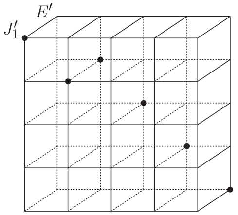
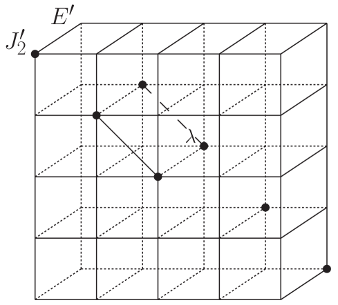
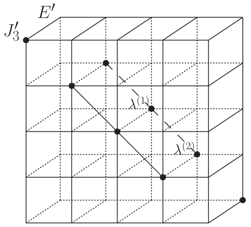
Figure 1: The three cubic grids are the pictorial description of $(E^{\prime},J_{i}^{\prime})$, where the solid nodes represent 1 if not specified by $\lambda$, and the blank nodes are zeroes. Here $\lambda,\lambda^{\scriptscriptstyle(1)},\lambda^{\scriptscriptstyle(2)}\neq\{0,1\}$.

Now all the parameters are sorted into two categories: one including the redundant parameters, which can be eliminated out of the states through ILOs ($\lambda$s in $(E,J_{1})$); the other possesses nonlocal properties (properties invariant under ILOs) which can not be eliminated through the ILOs and will keep staying in the entangled states as continuous parameters ($\lambda$s in $(E,J_{2}^{\prime}),(E,J_{3}^{\prime})$ ). However, there exist residual symmetries on the nonlocal parameters under ILOs. Take the entanglement class $(E^{\prime},J_{2}^{\prime})$ in Fig.(1) as an example, there exist the following transformations

$$\begin{pmatrix}\text{diag}\{0,1,\lambda,1,1\}\\ \text{diag}\{1,1,1,0,0\}\end{pmatrix} \xrightarrow{F} \begin{pmatrix}\text{diag}\{0,1,\frac{1}{\lambda},1,1\}\\ \text{diag}\{1,1,1,0,0\}\end{pmatrix}\;,$$ (9)

$$\begin{pmatrix}\text{diag}\{0,1,\lambda,1,1\}\\ \text{diag}\{1,1,1,0,0\}\end{pmatrix} \xrightarrow{G} \begin{pmatrix}\text{diag}\{0,1,1\!-\!\lambda,1,1\}\\ \text{diag}\{1,1,\hskip 8.5359pt1\hskip 8.5359pt,0,0\}\end{pmatrix}\;.$$ (10)

Here, transformation $G,F$ can be realized by the following ILOs:

$$G = T\otimes P\otimes Q$$ (11)

$$= \begin{pmatrix}-1&1\\ 0&1\end{pmatrix}\otimes\begin{pmatrix}0&1&0&0&0\\ 1&0&0&0&0\\ 0&0&1&0&0\\ 0&0&0&-1&0\\ 0&0&0&0&-1\end{pmatrix}\otimes\begin{pmatrix}0&1&0&0&0\\ 1&0&0&0&0\\ 0&0&1&0&0\\ 0&0&0&1&0\\ 0&0&0&0&1\end{pmatrix}\;,$$

$$F = T\otimes P\otimes Q$$ (12)

$$= \begin{pmatrix}\frac{1}{\lambda}&0\\ 0&1\end{pmatrix}\otimes\begin{pmatrix}1&0&0&0&0\\ 0&0&1&0&0\\ 0&1&0&0&0\\ 0&0&0&\lambda&0\\ 0&0&0&0&\lambda\end{pmatrix}\otimes\begin{pmatrix}1&0&0&0&0\\ 0&0&1&0&0\\ 0&1&0&0&0\\ 0&0&0&1&0\\ 0&0&0&0&1\end{pmatrix}\;,$$

where $T,P,Q$ act on the quantum state as in Eq.(4). The transformed entangled states under $F,G$ are SLOCC equivalent with their initial states. If we assign

$$F(\lambda)=\frac{1}{\lambda}\;,\;G(\lambda)=1-\lambda\;,$$

$$FG(\lambda)=F(G(\lambda))=\frac{1}{1-\lambda}\;,$$ (13)

then the $F,G$ operations generate a group, i.e., $\{E,F,G,GFG,FG,GF\}$, which is isomorphic to $S_{3}$ group [16].

Considering the general case of $(E^{\prime},J^{\prime})$ in Eq.(8), we can represent the $m-2$ parameters in a row vector

$$(\lambda^{(1)},\cdots,\lambda^{(m-2)})\doteq\begin{pmatrix}\text{diag}\{0,1,\lambda^{(1)},\lambda^{(2)},\cdots,\lambda^{(m-2)},1,\cdots,1\}\\ \text{diag}\{1,1,1\hskip 11.38092pt,1\hskip 14.22636pt,\cdots,\hskip 8.5359pt1\hskip 17.07182pt,\,0,\cdots,0\}\end{pmatrix}\;.$$ (14)

Here $\doteq$ means represented. Define

$$A_{i}(\lambda^{(1)},\cdots,\lambda^{(i)},\lambda^{(i+1)},\cdots,\lambda^{(m-2)}) = (\lambda^{(1)},\cdots,\lambda^{(i+1)},\lambda^{(i)},\cdots,\lambda^{(m-2)})\;,$$ (15)

$$F(\lambda^{(1)},\cdots,\lambda^{(m-2)}) = (\frac{\lambda^{(1)}}{\lambda^{(m-2)}},\frac{\lambda^{(2)}}{\lambda^{(m-2)}},\cdots,\frac{1}{\lambda^{(m-2)}})\;,$$ (16)

$$G(\lambda^{(1)},\cdots,\lambda^{(m-2)}) = (1-\lambda^{(1)},\cdots,1-\lambda^{(m-2)})\;,$$ (17)

where all the transformation $A,F,G$ can be realized as that of Eqs.(12,11). If we assign the operators $A_{i}=\sigma_{i},F=\sigma_{m-2},G=\sigma_{m-1}$, it can be verified that

$$\left\{\begin{aligned} \sigma_{i}^{2}&=1\;\\ \sigma_{i}\sigma_{j}&=\sigma_{j}\sigma_{i}\hskip 28.45274pt\text{if $|j-i|\geq 2$}\;\\ \sigma_{i}\sigma_{i+1}\sigma_{i}&=\sigma_{i+1}\sigma_{i}\sigma_{i+1}\end{aligned}\right.\;.$$ (18)

These are the generators of the $S_{m}$ symmetric group. If the dimension $N=m+1$, then there is another additional symmetry operation $H=\sigma_{m}$ where

$$H(\lambda^{(1)},\cdots,\lambda^{(m-2)})=(\frac{1}{\lambda^{(1)}},\cdots,\frac{1}{\lambda^{(m-2)}})\;,$$ (19)

then$(A_{i},F,G,H)$ will generate an $S_{m+1}$ group.

3 The total number of the entanglement classes

Regard the entanglement class with nonlocal parameters in a representative state (e.g., state $(E^{\prime},J_{2}^{\prime})$ in Fig.(1)) as one continuous class, we have shown that there are 61 classes in $2\times 6\times 7$ states [13]. In our classification schemes, the number of the entanglement classes of sets $c_{N,l}$ in [12] (or $c_{M,l}$ in [13]) can be counted by the number of Jordan forms, which are characterized by Segre symbols. There is one case that do not correspond to the true tripartite entanglement in $c_{N,l}$ with $(E,J)$ where $J=[(\underbrace{11\cdots 11}_{N})]$. This corresponds to the following case

$$\begin{pmatrix}E\\ J\end{pmatrix}=\begin{pmatrix}\text{diag}\{1,1,\cdots,1,1\}\\ \text{diag}\{1,1,\cdots,1,1\}\end{pmatrix}\;,$$ (20)

which is actually a bipartite $N\times N$ entangled state. It is known that the generating function of the number of Segre symbols $S(n)$ for $n\times n$ matrix is [17]

$$\prod_{i=1}^{\infty}\frac{1}{(1-x^{i})^{P(i)}}=\sum_{n}S(n)x^{n}\;,$$ (21)

where $P(i)$ is the number of partitions of integer $i$.

Consider the general entanglement sets $c_{M-i,l}$ of $2\times M\times N$ system. The canonical form of the matrix pair $\left(\begin{smallmatrix}\Gamma_{\!1}\\ \Gamma_{\!2}\end{smallmatrix}\right)\in c_{M-i,l}$ has the following forms (see Eq.(49) of Ref.([13]))

$$\Gamma_{\!1}=\left(\begin{array}[]{lll}E_{\scriptstyle(M-i)\times(M-i)}&{\bf 0}&{\bf 0}\\ {\bf 0}&{\bf 0}_{\scriptstyle i\times i}&{\bf 0}_{\scriptstyle i\times(N-M)}\\ \end{array}\right)\;,$$ (24)

and

$$\Gamma_{\!2}=\left(\begin{array}[]{ll}J_{d_{J}}&{\bf 0}\\ {\bf 0}&B_{(M-d_{J})\times(N-d_{J})}\end{array}\right)\;,$$ (27)

where $d_{J}$ is the dimension of $J$ and ${\bf 0}$ are the zero submatrices, see Fig.(2). We can formally write the number of inequivalent classes of the sets $\{c_{M-i,l}\}$ by $\omega_{M,N}$ as follows

$$\omega_{M,N}(i,d_{J})=S(d_{J})\cdot F_{r_{B}}\;.$$ (28)

Here $r_{B}$ represents the rank of $B$, $F_{r_{B}}$ is the number of different forms of $B$ in $c_{M-i,l}$. The value of $F_{r_{B}}$ can be deduced from the construction procedures of $B$, see Fig.(2). If we know $B_{i}$ (see the submatrix outlined by the thick lines in (ii) of Fig.(2)), the $B^{(i+1)}$ then can be constructed based on the rank of $R,C$ of $B^{(i)}$. And the rank of $R^{\prime},C^{\prime}$ in $B^{(i+1)}$ must be less than or equal to that of $R,C$ separately (see (ii) of Fig.(2)). There will be three cases: (1), $r(C^{\prime})=0$, and all the $B$ matrices after $B^{(i+1)}$ will have $r(C^{\prime\prime})=0,\cdots$; (2), $r(R^{\prime})=0$ which is the similar to (1); (3), $r(C^{\prime})\neq 0$ and $r(R^{\prime})\neq 0$ which we can construct $B^{(i+2)}$ recursively. Translate this into mathematics, we can get the following recursive formula of the number of $F_{r_{B}}$

$$F_{r_{B}}=F(j,r,c)=F(j,r,0)+F(j,0,c)+\sum_{m=1}^{r}\sum_{n=1}^{c}F(j-m-n,m,n)\;,$$ (29)

where $r,c$ are the rank of $R,C$ associated with the corresponding $B$ submatrix and the initial values are $r=i,c=i+N-M$ separately; $j=r_{B}-i-(i+N-M)$; $F(j,r,0)=f_{j}^{(r)},F(j,0,c)=f_{j}^{(c)}$. Here $f_{n}^{(m)}$ is the number of partitions of $n$ where the maximum part is $m$ whose generating function is

$$\prod_{k=1}^{m}\frac{1}{1-x^{k}}=\sum_{n}f_{n}^{(m)}x^{n}\;.$$ (30)

It can be verified that $F(0,r,c)=1$, and we assume $F(-j,r,c)=0$.

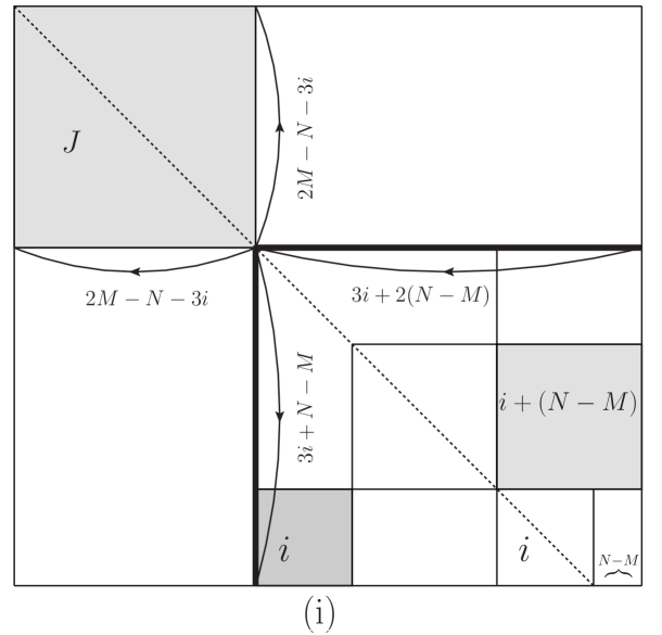
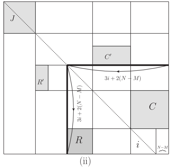
Figure 2: Two different forms of $\Gamma_{2}$ in Eq.(27). The thick lines outlines the $B$ matrix. (i) the initial $B$ matrix with the dimensions being labeled. (ii) In the next step of enlargement of $B$ matrix, the rank of submatrices $C^{\prime}$ and $R^{\prime}$ must be less than that of $R$ and $C$.

If the the initial matrix is $B_{(3i+N-M)\times(3i+2(N-M))}$ whose rank is $(2i+N-M)$, see (i) of Fig.(2), then there has only one form. Thus there are $S(2M-N-3i)$ inequivalent classes,

$$\omega_{M,N}(i,j=0) = S(2M-N-3i)\cdot F(j,R,C)$$ (31)

$$= S(2M-N-3i)\cdot F(0,i,i+(N-M))$$

$$= S(2M-N-3i)\cdot 1\;.$$

If the rank of $B$ enlarged to $j+(2i+N-M)$, we have the number of inequivalent classes $\omega_{M,N}(i,j)$ to be

$$\omega_{M,N}(i,j)=S(2M-N-3i-j)\cdot F(j,i,i+(N-M))\;.$$ (32)

Specifically when $M=N$ and $i=j=0$, there is one case that does not correspond to true entanglement (see Eq.(20)). Thus the total number of inequivalent entanglement classes $\Omega(M,N)$ can be derived

$$\Omega_{M,N}=\sum_{i=0}^{\scriptstyle\lfloor\frac{2M-N}{3}\rfloor}\,\sum_{j=0}^{\scriptstyle(2M-N-3i)}\omega_{M,N}(i,j)-\delta_{MN}\;.$$ (33)

The above equation can be evaluated by computers for arbitrary given $M$ and $N$. The values of $\Omega_{M,N}$ up to $2\times 10\times 10$ are listed in Table (1).

	2	3	4	5	6	7	8	9	10
2	2	2	1	1	1	1	1	1	1
3	2	6	5	2	1	1	1	1	1
4	1	5	16	12	6	2	1	1	1
5	1	2	12	34	28	14	6	2	1
6	1	1	6	28	77	61	34	15	6
7	1	1	2	14	61	157	133	74	36
8	1	1	1	6	34	133	328	277	165
9	1	1	1	2	15	74	277	655	572
10	1	1	1	1	6	36	165	572	1309

Table 1: The number of inequivalent classes of true tripartite entanglement system of $2\times M\times N$ up to $10$.

From the table, it can be confirmed that the number of entanglement classes of $2\times N\times N$ system increases exponentially with the dimensions of system, i.e., $\Omega_{N,N}\sim 2^{N}$.

4 Conclusions

In this paper we have investigated two interesting features of the entanglement classes of $2\times M\times N$ system. The continuous entanglement classes with more than one nonlocal parameters come into existence, and there exits a upper limit for the number of nonlocal parameters. Meanwhile, there are some residual discrete symmetries that remain exist under continuous ILO transformations of $SL(2,\mathbb{C}),SL(M,\mathbb{C}),SL(N,\mathbb{C}),$ which are isomorphic to symmetry groups. We also get an analytic expression for the total number of inequivalent entanglement classes where the same structured entanglement class with continuous parameters are regard as the same class, and it indicates that the entanglement classes are generally exponentially increasing with the dimensions in $2\times N\times N$ system. With these results, the full understanding of the entanglement classes of $2\times M\times N$ thus becomes promising. It is worth mentioning that the classification of $2\times M\times N$ may shed some light on the classification of other entangled systems, e.g. the entangled $(2N+1)$-qubit system.

Appendix

Appendix A Proof of Proposition 2.1

Proof:

Consider the following entangled class in Eq.(5)(with $N-m>1$)

$$\begin{pmatrix}E\\ J\end{pmatrix}=\begin{pmatrix}\text{diag}\{\;1\,,\hskip 2.84544pt1\,,\cdots\,,\hskip 2.84544pt1\hskip 5.69046pt,\underbrace{1,\cdots,1}_{N-m}\}\\ \text{diag}\{\lambda_{1},\lambda_{2},\cdots\,,\lambda_{m},\overbrace{0,\cdots,0}\}\end{pmatrix}\in c_{N,m}\;,$$

the ILO transformations $T,P,Q$ that apply on this class would transform it into other forms, i.e., $(E,J^{\prime})$. But standard form of $(E,J^{\prime})$ must be also in the set $c_{N,m}$, so we have

$$\begin{pmatrix}E\\ J^{\prime}\end{pmatrix}=\begin{pmatrix}\text{diag}\{\;1\,,\hskip 2.84544pt1\,,\cdots\,,\hskip 2.84544pt1\hskip 5.69046pt,\underbrace{1,\cdots,1}_{N-m}\}\\ \text{diag}\{\lambda^{\prime}_{1},\lambda^{\prime}_{2},\cdots\,,\lambda^{\prime}_{m},\overbrace{0,\cdots,0}\}\end{pmatrix}\in c_{N,m}\;.$$

It is easy to verify that the operation $T,P,Q$ which makes

$$(E,J)\xrightarrow{T,P,Q}(E,J^{\prime})\;,$$

will leads to $\lambda^{\prime}=\frac{t_{22}\lambda}{t_{11}+t_{12}\lambda}$, here $t_{ij}$ are matrix elements of $T$ see Eq.(38) in [12]. Here we neglect the subscripts of $\lambda$s and $\lambda^{\prime}$s, for there can be a change of the orders of different $\lambda^{\prime}$s induced by $P,Q$ operations. We conclude that the ILO transformations ($T,P,Q$) induce a special linear fraction transformations which keep $0$ invariant (i.e., $\lambda^{\prime}=\frac{t_{22}\lambda}{t_{11}+t_{12}\lambda}$) on the eigenvalues of $J$ in the entangled class $(E,J)$.

We apply the different ILO transformations introduced in Eqs.(6,7), the entangled state ($(E,J)\in c_{N,m}$) is thus transformed into the form of Eq.(8). In this form, there are $m-2$ $(m\geq 3)$ parameters $\lambda^{(k)}$, where $\lambda^{(k)}=\frac{0-\lambda_{2}}{0-\lambda_{k+2}}\cdot\frac{(\lambda_{1}-\lambda_{k+2})}{(\lambda_{1}-\lambda_{2})}$ is the cross ratio of $(0,\lambda_{1},\lambda_{2},\lambda_{k+2})$. Combined with the argument in the previous paragraph, we have

Proposition A.1

The cross ratio $\lambda^{(k)}$ is invariant under ILOs.

Now we proceed to prove Proposition 2.1. Suppose the $m-2$ $\lambda^{(i)}$ can be further transformed into a form with $m-2-l$ parameters $\lambda^{\prime(i)}$ via ILOs, where $l\geq 1$, then we would have the following $m-2-l$ equations

$$\lambda^{\prime(1)} = \lambda^{\prime(1)}(\lambda^{(1)},\cdots,\lambda^{(m-2)})\;,$$

$$\cdots$$

$$\lambda^{\prime(m-2-l)} = \lambda^{\prime(m-2-l)}(\lambda^{(1)},\cdots,\lambda^{(m-2)})\;.$$

Clearly there are less equations (there are $m-2-l$) than parameters $\lambda^{(i)}$ (there are $m-2$). At least, there exists a parameter, suppose $\lambda^{(k)}$, that can not be determined by the $m-2-l$ equations by $\lambda^{\prime(i)}$s. This is equivalent to say that the entangled states with continuous parameters $\lambda^{(k)}$ are all equivalent to the same entangled state specified by $\lambda^{\prime(i)}$s, therefore different value of $\lambda^{(k)}$ are themselves ILO equivalent which contradicts Proposition A.1. Thus we have the $m-2$ $\lambda^{(i)}$ in Eq.(8) are nonlocal parameters which can not be further eliminated by ILOs.

For the case of $N-m=1$, the proof is similar except inducing an additional symmetry in Eq.(19).

Acknowledgments

This work was supported in part by the National Natural Science Foundation of China(NSFC) under the grants 10935012, 10928510, 10821063 and 10775179, by the CAS Key Projects KJCX2-yw-N29 and H92A0200S2, and by the Scientific Research Fund of GUCAS.

References

[1] M.A. Nielsen and I.L. Chuang, Quantum Computation and Quantum Information (Cambridge
University Press, Cambridge, England, 2000).
[2] Ryszard Horodecki, Paweł Horodecki, Michał
Horodecki, and Karol Horodecki, Rev. Mod. Phys. 81, 865
(2009).
[3] Asher Peres, Phys. Rev. Lett. 77, 1413
(1996).
[4] Michał Horodecki, Paweł Horodecki, and Ryszard
Horodecki, Phys. Lett. A 223, 1 (1996).
[5] William K. Wootters, Phys. Rev. Lett. 80, 2245 (1998).
[6] W. Dür, G. Vidal, and J.I. Cirac, Phys. Rev. A 62, 062314 (2000).
[7] F. Verstraete, J. Dehaene, B. De Moor, and H.
Verschelde, Phys. Rev. A 65, 052112 (2002).
[8] L. Lamata, J. León, D. Salgado, and E.
Solano, Phys. Rev. A 75, 022318 (2007).
[9] Lin Chen and Yi-Xin Chen, Phys. Rev. A 73, 052310
(2006).
[10] Lin Chen, Yi-Xin Chen, and Yu-Xue Mei, Phys. Rev.
A 74, 052331 (2006).
[11] Marcio F. Cornelio and A. F. R. de Toledo Piza, Phys. Rev. A 73, 032314
(2006).
[12] Shuo Cheng, Junli Li, and Cong-Feng Qiao, J. Phys. A: Math. Theor. 43, 055303
(2010).
[13] Junli Li and Cong-Feng Qiao,
arXiv: 1001.0078(2010).
[14] Eric Chitambar, Carl A. Miller, and Yaoyun
Shi, arXiv: 0911.1803.
[15] Eric Chitambar, Carl A. Miller, and Yaoyun
Shi, arXiv: 0911.4058.
[16] Shuo Cheng, Junli Li, and Cong-Feng Qiao, Journal of the
Graduate School of the Chinese Academy of Sciences 3, 303
(2009) (in chinese).
[17] N. J. A. Sloane, The On-Line Encyclopedia of Integer Sequences,
published electronically at
www.research.att.com/~njas/sequences/, (2008).