Abstract

In this paper we investigate cosmological dynamics on the normal branch of a DGP-inspired scenario within a phase space approach where induced gravity is modified in the spirit of $f(R)$-theories. We apply the dynamical system analysis to achieve the stable solutions of the scenario in the normal DGP branch. Firstly, we consider a general form of the modified induced gravity and we show that there is a standard de Sitter point in phase space of the model. Then we prove that this point is stable attractor only for those $f(R)$ functions that account for late-time cosmic speed-up.
PACS: 04.50.-h, 95.36.+x, 98.80.-k
Key Words: Dark Energy, Braneworld Cosmology, Curvature Effects, Dynamical System, Induced Gravity

1 Introduction

There are many astronomical evidences supporting the idea that our universe is currently undergoing a speed-up expansion [1]. Several approaches are proposed in order to explain the origin of this novel phenomenon. These approaches can be classified in two main categories: models based on the notion of dark energy which modify the matter sector of the gravitational field equations and those models that modify the geometric part of the field equations generally dubbed as dark geometry in literature [2,3]. From a relatively different viewpoint (but in the spirit of dark geometry proposal), the braneworld model proposed by Dvali, Gabadadze and Porrati (DGP) [4] explains the late-time cosmic speed-up phase in its self-accelerating branch without recourse to dark energy [5]. However, existence of ghost instabilities in this branch of the solutions makes its unfavorable in some senses [6]. Fortunately, it has been revealed recently that the normal, ghost-free DGP branch has the potential to explain late-time cosmic speed-up if we incorporate possible modification of the induced gravity in the spirit of $f(R)$-theories [7]. This extension can be considered as a manifestation of the scalar-tensor gravity on the brane. Some features of this extension are studied recently [8,9].

Within this streamline, in this paper we study the phase space of the normal DGP cosmology where induced gravity is modified in the spirit of $f(R)$-theories. We apply the dynamical system analysis to achieve the stable solutions of the model. To achieve this goal, we firstly consider a general form of the modified induced gravity. We obtain fixed points via an autonomous dynamical system where the stability of these points depends explicitly on the form of the $f(R)$ function. There are also de Sitter phases, one of which is a stable phase explaining the late-time cosmic speed-up. Secondly, in order to determine the stability of critical points and for the sake of clarification, we specify the form of $f(R)$ by adopting some cosmologically viable models. The phase spaces of these models are analyzed fully and the stability of critical points are studied with details.

2 DGP-inspired $f(R)$ gravity

2.1 The basic equations

Modified gravity in the form of $f(R)$-theories are derived by generalization of the Einstein-Hilbert action so that $R$ (the Ricci scalar) is replaced by a generic function $f(R)$ in the action

$$S=\int d^{4}x\sqrt{-g}\Big{(}\frac{f(R)}{2\kappa^{2}}+{\bf L_{m}}\Big{)}\,,$$ (1)

where ${\bf L_{m}}$ is the matter Lagrangian and $\kappa^{2}=8\pi G$. Varying this action with respect to the metric gives

$$G_{\mu\nu}=\kappa^{2}T^{(tot)}_{\mu\nu}=\kappa^{2}\Big{(}T^{(m)}_{\mu\nu}+T^{(f)}_{\mu\nu}\Big{)}=\kappa^{2}\frac{\widetilde{T}^{(m)}_{\mu\nu}+\widetilde{T}^{(f)}_{\mu\nu}}{f^{\prime}}$$ (2)

where $\widetilde{T}^{(m)}_{\mu\nu}=diag(\rho,-p,-p,-p)$ is the stress-energy tensor for standard matter, which is assumed to be a perfect fluid and by definition $f^{\prime}\equiv\frac{df}{dR}$ . Also $\widetilde{T}^{(f)}_{\mu\nu}$ is the stress-energy tensor of the curvature fluid that is defined as follows

$$\widetilde{T}^{(f)}_{\mu\nu}=\frac{1}{2}g_{\mu\nu}\Big{[}f(R)-Rf^{\prime}\Big{]}+f^{\prime\,\,;\alpha\beta}(g_{\alpha\mu}g_{\beta\nu}-g_{\alpha\beta}g_{\mu\nu})\,.$$ (3)

By substituting a flat FRW metric into the field equations, one achieves the analogue of the Friedmann equations as follows [10]

$$3f^{\prime}H^{2}=\kappa^{2}\rho_{m}+\Big{[}\frac{1}{2}\Big{(}f(R)-Rf^{\prime}\Big{)}-3H\dot{f^{\prime}}\Big{]}$$ (4)

$$-2f^{\prime}\dot{H}=\kappa^{2}\rho_{m}+\dot{R}^{2}f^{\prime\prime\prime}+(\ddot{R}-H\dot{R})f^{\prime\prime}\,,$$ (5)

where a dot marks the differentiation with respect to the cosmic time. In the next step, following [9] we suppose that the induced gravity on the DGP brane is modified in the spirit of $f(R)$ gravity. The action of this DGP-inspired $f(R)$ gravity is given by

$$S=\frac{1}{2\kappa_{5}^{3}}\int d^{5}x\sqrt{-g}{\cal R}+\int d^{4}x\sqrt{-q}\bigg{(}\frac{f(R)}{2\kappa^{2}}+{\bf{L}}_{m}\bigg{)}\,,$$ (6)

where $g_{AB}$ is the five dimensional bulk metric with Ricci scalar ${\cal R}$, while $q_{ab}$ is induced metric on the brane with induced Ricci scalar $R$. The Friedmann equation in the normal branch of this scenario is written as [9]

$$3f^{\prime}H^{2}=\kappa^{2}\Big{(}\rho_{m}+\rho^{(f)}\Big{)}-\frac{3H}{r_{c}}\,,$$ (7)

where $r_{c}=\frac{G^{(5)}}{G^{(4)}}=\frac{\kappa_{5}^{2}}{2\kappa^{2}}$  is the DGP crossover scale with dimension of $[length]$ and marks the IR (infra-red) behavior of the DGP model. The Raychaudhuri’s equation is written as follows

$$\dot{H}\Big{(}1+\frac{1}{2Hr_{c}f^{\prime}}\Big{)}=-\frac{\kappa^{2}\rho_{m}}{2f^{\prime}}-\frac{\dot{R}^{2}f^{\prime\prime\prime}+(\ddot{R}-H\dot{R})f^{\prime\prime}}{2f^{\prime}}\,\,.$$ (8)

To achieve this equation we have used the continuity equation for $\rho^{(f)}$ as

$$\dot{\rho}^{(f)}+3H\bigg{(}\rho^{(f)}+p^{(f)}+\frac{\dot{R}f^{\prime\prime}}{r_{c}(f^{\prime})^{2}}\bigg{)}=\frac{\kappa^{2}\rho_{m}\dot{R}f^{\prime\prime}}{(f^{\prime})^{2}}\,,$$ (9)

where the energy density and pressure of the curvature fluid are defined as follows

$$\rho^{(f)}=\frac{1}{\kappa^{2}}\bigg{(}\frac{1}{2}\Big{[}f(R)-Rf^{\prime}\Big{]}-3H\dot{f^{\prime}}\bigg{)}\,,$$ (10)

$$p^{(f)}=\frac{1}{\kappa^{2}}\bigg{(}{2H\dot{f^{\prime}}+\ddot{f^{\prime}}-\frac{1}{2}\Big{[}f(R)-Rf^{\prime}\Big{]}}\bigg{)}\,.$$ (11)

After presentation of the required field equations, we analyze the phase space of the model fully to explore cosmological dynamics of this setup.

2.2 A dynamical system viewpoint

The dynamical system approach is a convenient tool to describe dynamics of cosmological models in phase space. In this way, we rewrite equation (7) in a dimensionless form as

$$1=\frac{\rho_{m}}{3H^{2}f^{\prime}}-\frac{1}{Hr_{c}f^{\prime}}+\frac{f(R)}{6H^{2}f^{\prime}}-\frac{R}{6H^{2}}-\frac{\dot{f^{\prime}}}{Hf^{\prime}}\,.$$ (12)

In the present study, we firstly consider a generic form of the $f(R)$ function, so that one can define the dynamical variables independent on the specific form of the $f(R)$ function as follows (see for instance Ref. [10])

$$x_{1}=\frac{\rho_{m}}{3H^{2}f^{\prime}}\,,\quad\ x_{2}=-\frac{1}{Hr_{c}f^{\prime}}\,,\quad\ x_{3}=\frac{f}{6H^{2}f^{\prime}}\,,\quad\ x_{4}=-\frac{R}{6H^{2}}\,,\quad\ x_{5}=-\frac{\dot{f^{\prime}}}{Hf^{\prime}}\,.$$ (13)

Also we define the following quantities

$$m\equiv\frac{d\ln{f^{\prime}}}{d\ln{R}}=\frac{Rf^{\prime\prime}}{f^{\prime}}$$ (14)

$$\quad\quad\ r\equiv-\frac{d\ln{f}}{d\ln{R}}=-\frac{Rf^{\prime}}{f}=\frac{x_{4}}{x_{3}}\,.$$ (15)

We note that a constant value of $m$ leads to the models with $f(R)=\xi_{1}+\xi_{2}R^{1+m}$ where the parameter $m$ shows the deviation of the background dynamics from the standard model and $\xi_{1}$ and $\xi_{2}$ are constants. However, in general the parameter $m$ depends on $R$ and $R$ itself can be expressed in terms of the ratio $r=\frac{x_{4}}{x_{3}}$ . This means that $m$ is a function of $r$, that is, $m=m(r)$. Based on the new variables, the Friedmann equation becomes a constraint equation so that we can express one of these variables in terms of the others. Introducing a new time variable $\tau=\ln{a}=N$  and eliminating $x_{1}$ (by using the Friedmann constraint equation) we obtain the following autonomous system

$$\frac{dx_{2}}{dN}=x_{2}(x_{5}+x_{4}+2)\,,\$$ (16)

$$\quad\quad\quad\quad\,\,\,\frac{dx_{3}}{dN}=-\frac{x_{4}x_{5}}{m}+x_{3}(2x_{4}+x_{5}+4)\,,\$$ (17)

$$\quad\,\,\,\frac{dx_{4}}{dN}=\frac{x_{4}x_{5}}{m}+x_{4}(2x_{4}+4)\,,\$$ (18)

$$\frac{dx_{5}}{dN}=(x_{2}+x_{5})(x_{5}+x_{4})+1-3x_{3}-5x_{4}-2x_{2}\,,\$$ (19)

and

$$x_{1}\equiv\Omega_{m}=1-x_{2}-x_{3}-x_{4}-x_{5}\,.\$$ (20)

The deceleration parameter which is defined as $q=-1-\frac{\dot{H}}{H^{2}}$ , now can be expressed as

$$q=1+x_{4}\,,\$$ (21)

and the effective equation of state parameter of the system is defined by

$$\omega_{eff}=-1-\frac{2\dot{H}}{3H^{2}}\,\,.$$ (22)

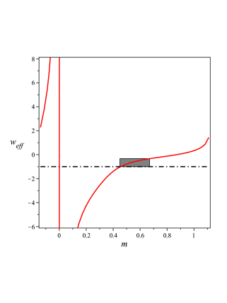
Figure 1: The effective equation of state parameter (left panel) and the deceleration parameter (right panel) of the critical point ${\cal E}$ versus $m$. The shaded region denotes a non-phantom acceleration era which occurs in the parametric space with $0.45<m<0.67$ . A slightly phantom-like behavior exists for $m<0.45$ and when $m\rightarrow 0$ , it reaches to a strong phantom-like phase. For negative values of $m$ the EoS parameter is stiff-like.

2.3 Critical points and their stability

The critical points of the scenario and some of their properties are listed in table $1$. In this table, $\Gamma$ is defined as

$$\Gamma\equiv\frac{1}{2}\,{\frac{4\,{m}^{2}-9\,m+2\pm\sqrt{-160\,{m}^{4}+272\,{m}^{3}-111\,{m}^{2}+4\,m+4}}{2\,{m}^{2}-3\,m+1}}\,.$$

We consider only the plus sign of this equation in our forthcoming arguments. The minus sign does not create suitable cosmological behavior since it leads to $w_{eff}<-10$ or $w_{eff}>0.7$ for point $\cal{E}$.

In table $1$, the critical points $\cal{A}$ , $\cal{B}$ and $\cal{C}$ are independent of the form of $f(R)$. Nevertheless, the stability of these points depends on the form of $f(R)$ explicitly. The critical curve ${\cal D}$ exists just for $f(R)$ models with $m(r=-\frac{1}{2})=\frac{1}{2}$ (for instance, in models of the form $f(R)=R+\gamma R^{-n}$  that $m$ is defined as $m(r)=-\frac{n(1+r)}{r}$,  the critical curve ${\cal D}$ exists just for $n=\frac{1}{2}$). The value of the effective equation of state parameter corresponding to this critical curve depends on the coordinate $x_{2}^{*}$ . Then, different intervals on this curve describe different era of the universe evolution (for example, a formal de Sitter-type era occurs for curve ${\cal D}$ at $x^{*}_{2}=-\frac{1}{4}$). Since the phase space behavior of the point ${\cal E}$ (with $m(r)=1+r$) depends on the form of $f(R)$ via $m$, we treat it separately in section $3$. In which follows, we classify the important subclasses in order to see their dynamical behaviors.

a) The radiation dominated era

The points ${\cal A}$ and ${\cal B}$ demonstrate effectively the radiation dominated epoch of the universe ($\omega_{eff}=\frac{1}{3}$ with $a(t)\propto t^{\frac{1}{2}}$). This phase can be realized also by the curve ${\cal D}$ for $x^{*}_{2}=\frac{5}{4}$ . The stability of these points is investigated in which follows.

b) The matter dominated era

The matter era ($\omega_{eff}=0$) could be existed for models with $m(r=-\frac{1}{2})=\frac{1}{2}$ by the localized point $x^{*}_{2}=\frac{7}{8}$ on the curve ${\cal D}$ . Note that this matter era is properly described by a cosmic expansion with scale factor $a(t)=a_{0}(t-t_{0})^{\frac{2}{3}}$. This era also can be realized in localized point $\cal{E}$ with $m(r=-0.13)=0.87$ .

c) The de Sitter era

The de Sitter phase ($\omega_{eff}=-1$) in the normal branch of this DGP-inspired $f(R)$ model is realized by the curve ${\cal C}$ of critical points. It is important to point out that the mentioned de Sitter solution is the standard de Sitter phase just for $x^{*}_{2}=2$ , since in this localized point the matter density parameter vanishes ($\Omega_{m}=0$). Also this phase can be realized from the curve of the non-localized points ${\cal D}$ with $x^{*}_{2}=-\frac{1}{4}$  (this de Sitter point can be regarded as the special case of the curve ${\cal C}$ in the localized point $x^{*}_{2}=-\frac{1}{4}$). But one can see that this point gives no standard de Sitter era since its $\Omega_{m}$ is non-vanishing (in this case $\Omega_{m}=0$ occurs at $x^{*}_{2}=\frac{1}{5}$).

d) Transition from $q>0$ to $q<0$

The critical point ${\cal E}$ depends explicitly on the form of $f(R)$ via $m$ and this is the case also for stability of this point. The point ${\cal E}$ describes a phase transition of the universe from deceleration to the acceleration era at $\omega_{eff}=-\frac{1}{3}$ and $q=0$  in this model for $m(r=-0.33)=0.67$ . Also the mentioned feature for $f(R)$ models with $m(r=-\frac{1}{2})=\frac{1}{2}$ (corresponding to the curve ${\cal D}$) occurs at the fixed point $x^{*}_{2}=\frac{1}{2}$ . So, one of the important feature of this model is that it clearly realizes the late-time acceleration of the universe in its normal branch for $0<m\leq 0.67$ . In figure $1$ the localized point ${\cal E}$ represents the deceleration phase for $m>0.67$ and a non-phantom accelerating phase for $0.45\leq m\leq 0.67$. For $m<0.45$ , since $q<-1$ , the model realizes an effective phantom phase with possibility of future big rip singularity which is characteristics of a non-canonical (phantom) field dominated universe. Similarly, the effective phantom behavior for the curve ${\cal D}$ occurs at $x^{*}_{2}<-\frac{1}{4}$ .

Table 1: Location, effective EoS and deceleration parameter of the critical points for the normal branch of a general DGP-inspired $f(R)$ scenario. The fixed point $\cal{D}$ exists only for those $f(R)$ models that $m(r=-\frac{1}{2})=\frac{1}{2}$.

point	$x_{2}$	$x_{3}$	$x_{4}$	$x_{5}$	$r$	$q$	$w_{eff}$
${\cal A}$	$0$	$\frac{17}{3}$	$0$	$-4$	$0$	$1$	$\frac{1}{3}$
${\cal B}$	$\frac{5}{4}$	$0$	$0$	$-2$	indefinite	$1$	$\frac{1}{3}$
${\cal C}$	$x^{*}_{2}$	$\frac{1}{3}(11-4x^{*}_{2})$	$-2$	$0$	$\frac{6}{4x^{*}_{2}-11}$	$-1$	$-1$
${\cal D}$	$x^{*}_{2}$	$-\frac{2}{3}(4x^{*}_{2}-5)$	$\frac{1}{3}(4x^{*}_{2}-5)$	$-\frac{1}{3}(1+4x^{*}_{2})$	$-\frac{1}{2}$	$\frac{2}{3}(2x^{*}_{2}-1)$	$\frac{1}{9}\Big{(}8x^{*}_{2}-7\Big{)}$
${\cal E}$	$0$	$\frac{\Gamma+4m}{2m(1-m)}$	$-\frac{\Gamma+4m}{2m}$	$\Gamma$	$m-1$	$-(1+\frac{\Gamma}{2m})$	$-\Big{(}1+\frac{\Gamma}{3m}\Big{)}$

In the next step we determine the stability of the critical points under small perturbations. The stability of these points is determined by the eigenvalues of the Jacobian matrix. For a general $f(R)$ term on the brane, stability of the critical points depends on the form of $f(R)$ (or equivalently on the parameter $m$). It is obvious that in general $m=m(r)$ is not a constant; it is a function of other variables so that one can expand this function of curvature about any of the fixed points. The results of our investigation for stability of critical points mentioned in table $1$, are summarized as follows:

$\bullet$   Point ${\cal A}$

As has been mentioned, this point is a radiation dominated era. In this case the eigenvalues are

$$-2\,,\,\,\frac{4(m-1)}{m}\,,\,\,-4\pm\,i\,.$$ (23)

Note that around this point, $m\equiv m_{\cal{A}}=m(r=0)$ . Hence this point is a spiral attractor if $0<m(r=0)<1$ , otherwise it is a saddle point. The corresponding 2D phase space for arbitrary $m=m(r)$ is shown in figure $2$ (left panel). Note that the Jacobian matrix in this point has no dependence on the $m^{\prime}(r)$  since this point lies around $r=0$. Here a prime denotes derivative with the respect to $r$ .

$\bullet$   Point ${\cal B}$

This point is also a radiation dominated era in which the eigenvalues are as follows

$$\lambda_{1,2}=-\frac{1}{8}(11\pm\sqrt{199}\,i)$$

$$\lambda_{3,4}={\frac{3\,m^{2}-m+m^{\prime}r(1+r)}{m^{2}}\pm\frac{\sqrt{(m^{2}-m)^{2}+2\,m^{\prime}r{m}^{2}(1-r)-2\,mm^{\prime}r(1+r)+{m^{\prime}}^{2}(r+{r}^{2})^{2}}}{m^{2}}}\,,$$ (24)

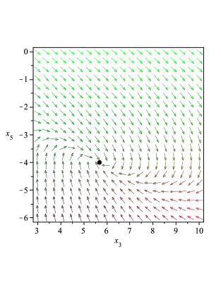
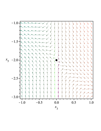
Figure 2: The phase subspace $x_{3}$ - $x_{5}$ of our setup at $x_{2}=x_{4}=0$ (left panel) and $x_{2}=\frac{5}{4}$ and $x_{4}=0$ (right panel) . The critical point shown in the left panel is point ${\cal A}$ and in the right panel it is point ${\cal B}$. Point ${\cal A}$ in the mentioned subspace is a spiral attractor and point ${\cal B}$ is a saddle point. Note that in the 4D phase space these are either spiral attractor or saddle point depending on the form of $f(R)$ .

where the parameter $m$ should be expanded around the point ${\cal B}$ (that is, $m=m_{\cal{B}}$). Here the stability issue depends also on $m$ and $m^{\prime}$, so that this point can be either a saddle or a spiral attractor. The corresponding 2D phase space for arbitrary $m=m(r)$ is shown in figure $2$ (right panel). An important point should be emphasized here: by setting $x_{4}=0$ in plotting figures $2$, their dependence on $m(r)$ is wasted. However, the situation is different if one plots the 3D subspace $x_{3}$ - $x_{4}$ - $x_{5}$ for these points. In this case, one should determine the form of the function $m(r=\frac{x_{4}}{x_{3}})$. For a constant $m$, the eigenvalues reduce to (2 , $-\frac{1}{8}(11\pm\sqrt{199}\,i)$ , $\frac{2(2m-1)}{m}$ ) which indicates that the point ${\cal B}$ is a saddle point for constant values of $m$.

$\bullet$   Curve ${\cal C}$

Generally, if a nonlinear system has a critical curve, the Jacobian matrix of the linearized system at a critical point on the line has a zero eigenvalue with an associated eigenvector tangent to the critical curve at the chosen point. When dynamical variables are not independent, some eigenvalues of the Jacobian matrix are zero. In this case, the phase space of the nonlinear system reduces to a lower dimensional phase space. The stability of an specific critical point on the curve can be determined by the nonzero eigenvalues, because near this critical point there is essentially no dynamics along the critical curve (i.e., along the direction of the eigenvector associated with the zero eigenvalue). So, the dynamics near this critical point may be viewed in a reduced phase space obtained by suppressing the zero eigenvalue direction. On the other hand, such curves are actually normally hyperbolic [11,12]. We consider a point on the curve ${\cal C}$ with coordinates $(2,\,1,\,-2,\,0)$. This point is a standard de Sitter phase. The eigenvalues corresponding to this point are as follows

$$0,\,\,\,\,\,\frac{1}{3}\Big{(}\chi-\frac{17}{\chi}-4\Big{)},\,\,\,\,\,-\frac{1}{6}\Big{(}\chi-\frac{17}{\chi}+8\Big{)}\pm i\frac{\sqrt{3}}{6}\Big{(}\chi+\frac{17}{\chi}\Big{)}\,,$$ (25)

where $\chi$ is defined as

$$\chi={\frac{\Big{[}\left(-460\,m+54+3\,\sqrt{3}\sqrt{8019\,{m}^{2}-1840\,m+108}\right){m}^{2}\Big{]}^{\frac{1}{3}}}{m}}.$$ (26)

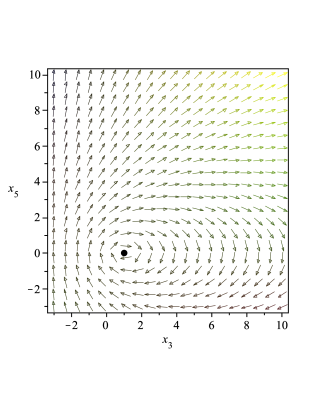
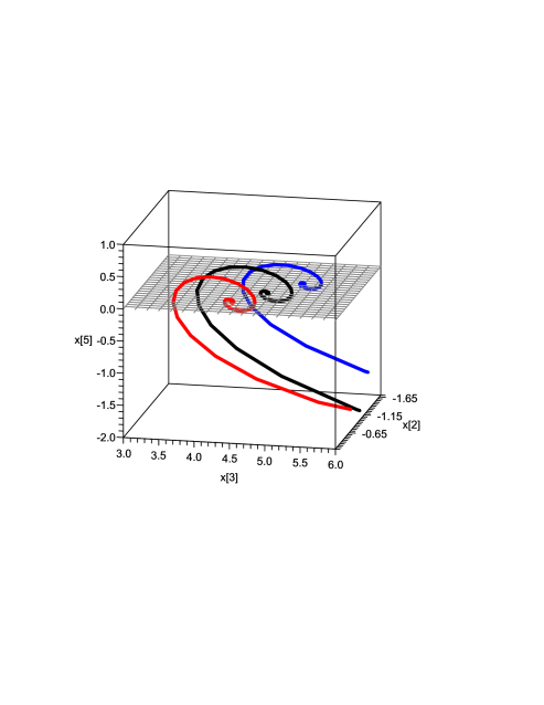
Figure 3: 2D phase space $x_{3}$ - $x_{5}$ for $x_{2}=2$ and $x_{4}=-2$ (left panel) and the 3D phase space $x_{2}$ - $x_{3}$ - $x_{5}$ for $x_{4}=-2$ (right panel). The critical point which is shown in the left panel is a center and is related to the standard de Sitter phase. The critical points shown in the right panel which lie on the line $x_{3}=\frac{1}{3}(11-4x_{2})$ are spiral attractors. These figures are plotted for $m(r=-2)=\frac{1}{2}$.

The parameter $m$ should be expanded around the standard point of ${\cal C}$ as defined previously with $m_{\cal{C}}=m(r=-2)$. Here the stability issue depends only on $m$. It is a stable spiral in the subspace of the last two eigenvalues when $0<m$. On the other hand, the second eigenvalue is negative for $m<0$ and $0.09\leq m$. So the standard de Sitter point in the $4$D phase space is a spiral attractor if

$$m\geq 0.09\,.$$ (27)

This point for other values of $m$ is a saddle point. Figure 3 shows the $2$D and $3$D phase spaces of the critical curve ${\cal C}$. We note that in the $2$D subspace, the de Sitter curve is reduced to a de Sitter point (as figure $3$ shows, this point is a center). Therefore, the center manifold theory is required to investigate its stability [13,14]. In $3$D subspace (right panel), the non-localized points in the $x_{2}$ - $x_{3}$ plane lie on the line $x_{3}=\frac{1}{3}(11-4x_{2})$. Figure $3$ is plotted for $m=\frac{1}{2}$ which satisfies (27), therefore this curve is a spiral de Sitter attractor.

3 Analytical results for some specific models

As we have mentioned previously, $m$ is a function of $r$, that is, $m=m(r)$. Since the $\Lambda$CDM model defined with $f(R)=R-2\Lambda$, corresponds to $m=0$, we can say that the quantity $m$ characterizes the deviation of the background dynamics from the standard $\Lambda$CDM model. Now we consider two specific model of $f(R)$ in order to obtain more obvious results. We also focus on the cosmological viability of these models. A cosmologically viable scenario contains an early time radiation dominated era followed by a matter dominated era that reaches to a standard de Sitter phase which is a stable attractor. We focus here only on the last two stages: matter domination and then a stable de Sitter attractor. At the first stage, the existence of a matter dominated era ( $w_{eff}=0$ ) constrains our DGP-inspired $f(R)$ model only to those $f(R)$ functions that $m(r=-\frac{1}{2})=\frac{1}{2}$ and $m(r=-0.13)=0.87$ (see table 1). In the first case, there exist two de Sitter phases: the localized point $x_{2}^{*}=-\frac{1}{4}$ on the curve ${\cal D}$ which is a formal de Sitter point, and also the de Sitter curve ${\cal C}$ which realizes a standard de Sitter point at the localized point $x^{*}_{2}=2$. The second case is associated just to the de Sitter curve ${\cal C}$. A correct connection between the unstable matter dominated era and the stable, standard de Sitter era is necessary condition for cosmological viability of a scenario. This connection can be investigated in the $m-r$ plane.

A)   $f(R)=R+\gamma R^{-n}$

For this model, the parameter $m$ takes the following form

$$m(r)=\frac{-n(1+r)}{r}\,,$$ (28)

which is independent on $\gamma$ . On the other hand, the point ${\cal E}$ of table $1$ is characterized by the following relation

$$m(r)=r+1\,.$$ (29)

Equations (28) and (29) give two solutions $m_{1}=0$ and $m_{2}=1-n$  for $m$. So, for the mentioned $f(R)$ function, point ${\cal E}$ is characterized by the following relation

$${\cal E}_{(1-n)}:\quad\Bigg{(}0,\,\frac{\Gamma^{(1-n)}+4(1-n)}{2n(1-n)}\,,\ -\frac{\Gamma^{(1-n)}+4(1-n)}{2(1-n)}\,,\ \Gamma^{(1-n)}\Bigg{)}\,,\,\,\,\,\,\,\omega_{eff}=-1-\frac{\Gamma^{(1-n)}}{3(1-n)}\,,$$ (30)

where $\Gamma^{(1-n)}\equiv\Gamma|_{m=1-n}$.

Note that the critical point ${\cal E}$ for $m=0$ (that is, ${\cal E}_{(0)}$) is indefinite and therefore we exclude it from our considerations. Now we investigate the stability of the critical point ${\cal E}_{(1-n)}$. Since the EoS parameter corresponding to this point varies with $m$, in order to determine the stability of this point, one has to fix the value of $m$.
In figure $4$ (left panel), we have shown the behavior of the parameter $m$ as a function of $r$ for a special $f(R)$ model given as $f(R)=R+\gamma R^{n}$  with  $n=0.13$ . As this figure shows, this model contains a connection between the matter era and the standard de Sitter era which is located at $m=-0.065$. However, this model is not cosmologically viable since it reaches an unstable standard de Sitter era. In figure $4$ (right panel), we plotted the curve $m(r)$ for $f(R)=R+\gamma R^{n}$ with $n=\frac{1}{2}$. The matter dominated era evolves to the standard de Sitter era at $m=-0.25$  which indicates that the standard de Sitter era is unstable (see Eq. (27)). So, this model is not cosmologically viable too. Note that in the right panel of figure $4$, the point $A$ lies also on the dashed line which is corresponding to the critical point ${\cal E}$. This feature indicates that this model contains the critical point ${\cal E}$ with $m(r=-\frac{1}{2})=\frac{1}{2}$ which is a non-phantom acceleration phase (compare this case with figure $1$ that $m=\frac{1}{2}$ lies in the shaded region).

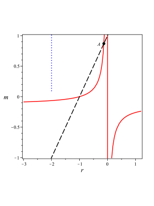
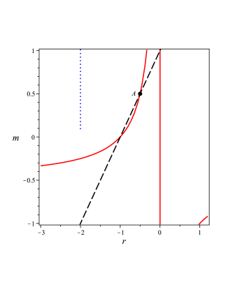
Figure 4: The solid curves illustrate the diagram $m-r$ of $f(R)=R+\gamma R^{-n}$ with $n=0.13$ (left panel) and with $n=\frac{1}{2}$ (right panel). The dashed-line is corresponding to the point ${\cal E}$ of table 1. The intersection point $A$ shows a matter domination phase. The standard de Sitter phase is corresponding to the line $r=-2$ and dotted (blue) line indicates the line of stability.

B)   $f(R)=R^{{}^{n}}\exp(\frac{\eta}{R})$

In this model the parameter $m$ is defined as

$$m(r)=-\frac{n+r(2+r)}{r}\,,$$ (31)

which is independent on $\eta$ . As has been pointed out previously, the matter dominated era can be achieved from critical point ${\cal E}$ in which the relative parameter is given by equation (29). Equating (29) and (31), we obtain two solutions for $m$ as $m=\frac{1\pm\sqrt{9-8n}}{4}$ .

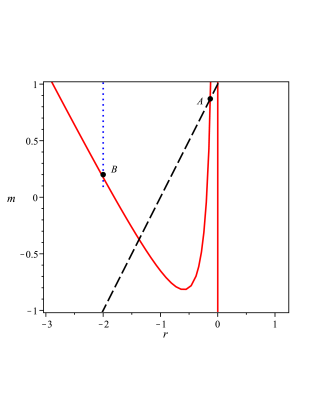
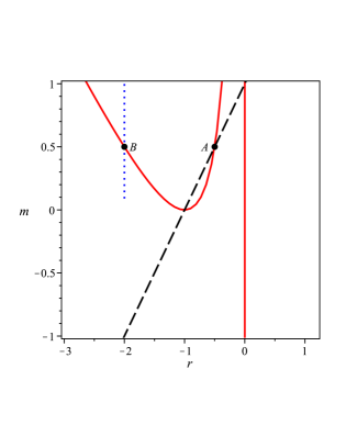
Figure 5: The diagram $m-r$ for $f(R)=R^{n}\exp(\frac{\eta}{R})$ with $n=0.35$ (left panel). The dashed-line shows the $m(r)$ function of the critical point ${\cal E}$. The intersection point $A$ shows a matter domination phase. This model reaches to the standard de Sitter phase at $B$ with $m=0.2$ which is a stable point. In this model the matter dominated era can be realized only by ${\cal E}$.

Now, the critical point ${\cal E}$ gives a matter dominated phase (with $m(r=-0.13)=0.87$) if we set $n=0.35$, that is to say, if $f(R)=R^{{}^{0.35}}\exp(\frac{\eta}{R})$ . In the model with $f(R)=R\exp(\frac{\eta}{R})$ (models with $m(r=-\frac{1}{2})=\frac{1}{2}$), the matter dominated era is realized by the curve ${\cal D}$ and the critical point ${\cal E}$ plays the role of a non-phantom acceleration era. In figure $5$ (left panel), the curve $m(r)$ is plotted for $f(R)=R^{{}^{0.35}}\exp(\frac{\eta}{R})$ . This model reaches the standard de Sitter phase at $m=0.2$ . Therefore, this point is stable since it belongs to the region defined by relation (27). Finally, we plot the $m(r)$ curve for $f(R)=R\exp(\frac{\eta}{R})$ as shown in the right panel of figure $5$. In this case there is an acceptable connection between the matter dominated era and the standard de Sitter phase since the standard de Sitter point at $m=\frac{1}{2}$ is a stable attractor. We note also that in this DGP-inspired $f(R)$ model there is a non-phantom acceleration phase which emerges from the point ${\cal E}$ with $m(r=-\frac{1}{2})=\frac{1}{2}$. This is corresponding to the point $A$ of figure $5$ (right panel).

4 Summary and Conclusion

In this paper we investigated cosmological dynamics of the normal DGP setup in a phase space approach where the induced gravity is modified in the spirit of $f(R)$-theories. The motivation for this study within a dynamical system approach lies in the fact that recently it has been revealed that the normal, ghost-free DGP branch has the potential to explain late-time speed-up if we incorporate possible modification of the induced gravity in the spirit of $f(R)$-theories. In this respect, a phase space analysis of the scenario would be interesting to reveal some aspects of this late-time behavior. Especially the stability of this late-time de Sitter phase is important to have a cosmologically viable solution. We applied the dynamical system analysis to achieve the stable solutions of the scenario in the normal DGP branch. We have shown that generally there are some fixed points that one of those is the standard de Sitter phase. Therefore, the normal branch of this DGP-inspired braneworld scenario realizes the late-time acceleration phase of the universe expansion. However, the stability of this point depends on the form of $f(R)$ via the parameter $m\equiv\frac{d\ln{f_{,{R}}}}{d\ln{R}}$. Then, we investigated the cosmological viability of these setups. A cosmologically viable scenario contains an early time radiation dominated era followed by a matter dominated era that reaches a standard de Sitter phase which is a stable attractor. Here we focused only on the last two stages: matter domination era followed by a stable de Sitter attractor. To be more specific, we considered two models with $f(R)=R+\gamma R^{n}$ and $f(R)=R^{n}\exp(\frac{\eta}{R})$ in our DGP-inspired setup. The condition for existence of the matter domination era restricted us to consider two cases $n=0.13$ and $n=\frac{1}{2}$ for the first model and two cases $n=0.35$ and $n=1$ for the second one. On the other hand, it is shown that the standard de Sitter phase is stable just for $m\geq 0.09$. So, since the first model reaches the standard de Sitter phase (which is determined by the line $r=-2$) at $m<0.09$ , it is not a cosmologically viable model. However, since the second model reaches this phase at $m>0.09$, it is a cosmologically viable model for $n=0.35$ and $n=1$.

References

-
[1]
S. Perlmutter et al, Astrophys. J. 517 (1999) 565
A. G. Riess et al, Astron. J. 116 (1998) 1006
D. N. Spergel et al, Astrophys. J. Suppl. 170 (2007) 377
E. Komatsu et al. [WMAP Collaboration], Astrophys. J. Suppl. 180 (2009) 330. -
[2]
E. J. Copeland, M. Sami and S. Tsujikawa, Int. J. Mod. Phys. D
15 (2006) 1753
V. Sahni and A. Starobinsky, Int. J. Mod. Phys. D 15 (2006) 2105
T. Padmanabhan, Gen. Rel. Grav. 40 (2008) 529
M. Sami, Curr. Sci. 97 (2009) 887. -
[3]
H. Kleinert and H. -J. Schmidt, Gen. Rel. Grav. 34 (2002) 1295
S. Nojiri and S. D. Odintsov, Int. J. Geom. Meth. Mod. Phys. 4 (2007) 115
T. P. Sotiriou and V. Faraoni, Rev. Mod. Phys. 82 (2010) 451
S. Capozziello and M. Francaviglia, Gen. Relativ. Gravit. 40 (2008) 357
R. Durrer and R. Maartens, Gen. Rel. Grav. 40 (2008) 301
S. Capozziello and V. Salzano, Adv. Astron. 1 (2009), [arXiv:0902.0088]
S. Capozziello, M. De Laurentis and V. Faraoni, [arXiv:0909.4672]
S. Nojiri and S. D. Odintsov, Phys. Rept. 505 (2011) 59. -
[4]
G. Dvali, G. Gabadadze and M. Porrati, Phys. Lett. B 485 (2000)
208
G. Dvali and G. Gabadadze, Phys. Rev. D 63 (2001) 065007
G. Dvali, G. Gabadadze, M. Kolanovi and F. Nitti, Phys. Rev. D 65 (2002) 024031. -
[5]
C. Deffayet, Phys. Lett. B 502 (2001) 199
C. Deffayet, G. Dvali and G. Gabadadze, Phys. Rev. D 65 (2002) 044023
A. Lue, Phys. Rept. 423 (2006) 1-48. -
[6]
K. Koyama, Class. Quantum Grav. 24 (2007) R231
C. de Rham and A. J. Tolley, JCAP 0607 (2006) 004. -
[7]
V. Sahni and Y. Shtanov, JCAP 0311 (2003) 014
A. Lue and G. D. Starkman, Phys. Rev. D 70 (2004) 101501
V. Sahni [arXiv:astro-ph/0502032]
L. P. Chimento, R. Lazkoz, R. Maartens and I. Quiros, JCAP 0609 (2006) 004
R. Lazkoz, R. Maartens and E. Majerotto, Phys. Rev. D74 (2006) 083510
R. Maartens and E. Majerotto, Phys. Rev. D74 (2006) 023004
M. Bouhmadi-Lopez, Nucl. Phys. B 797 (2008) 78. -
[8]
K. Nozari and M. Pourghassemi, JCAP 10 (2008) 044
J. Saavedra and Y. Vasquez, JCAP 04 (2009) 013
K. Atazadeh and H. R. Sepangi, Phys. Lett. B 643 (2006) 76
K. Atazadeh and H. R. Sepangi, JCAP 01 (2009) 006, [arXiv:0811.3823]
A. Borzou, H. R. Sepangi, S. Shahidi and R. Yousefi, EPL 88 (2009) 29001. -
[9]
M. Bouhmadi-Lopez, JCAP 0911 (2009) 011.
K. Nozari and F. Kiani, JCAP 07 (2009) 010. -
[10]
S. Nojiri and S. D. Odintsov, Phys. Rev. D 74 (2006) 086005
L. Amendola, D. Polarski and S. Tsujikawa, Phys. Rev. Lett. 98 (2007) 131302
S. Nojiri and S. D. Odintsov, J. Phys. Conf. Ser. 66 (2007) 012005
S. Capozziello, S. Nojiri, S. D. Odintsov and A. Troisi, Phys. Lett. B 639 (2006) 135
L. Amendola, D. Polarski and S. Tsujikawa, Int. J. Mod. Phys. D 16 (2007) 1555
L. Amendola, R. Gannouji, D. Polarski and S. Tsujikawa, Phys. Rev. D. 75 (2007) 083504
L. Amendola and S. Tsujikawa, Phys. Lett. B. 660 (2008) 125
B. Li and J. D. Barrow, Phys. Rev. D. 75 (2007) 084010. - [11] S. Y. Zhou, E. J. Copelend and P. M. Saffin, JCAP 07 (2009) 009.
- [12] M. Alimohammadi and A. Ghalee, Phys. Rev. D 80 (2009) 043006.
- [13] L. Perko, Differential Equations and Dynamical Systems, Springer-Verlag, New York, 1996
- [14] M. Abdelwahab, S Carloni and P. K. S. Dunsby, Class. Quant. Grav. 25 (2008) 135002.