Some recent studies of the AdS/CFT correspondence for condensed matter systems involve the Fermi liquid theory as a boundary field theory. Adding $B$-flux to the boundary D-branes leads in a certain limit to the noncommutative Fermi liquid, which calls for a field theory description of its critical behavior. As a preliminary step to more general consideration, the modification of the Landau’s Fermi liquid theory due to noncommutativity of spatial coordinates is studied in this paper. We carry out the renormalization of interactions at tree level and one loop in a weakly coupled fermion system in two spatial dimensions. Channels ZS, ZS’ and BCS are discussed in detail. It is shown that while the Gaussian fixed point remains unchanged, the BCS instability is modified due to the space non-commutativity.

April 2011

1 Introduction

Since more than ten years ago, noncommutative quantum field theory arising from string theory [1, 2, 3, 4] has received a great deal of attention. (For excellent reviews, see [5, 6]. For a reprint volume, see [7]. The Wightman axioms for noncommutative quantum field theory were studied in [8].) One of the most interesting results in the analysis of perturbative dynamics of noncommutative scalar field theories on a Euclidean space $\mathbb{R}^{4}$, is the existence of a mixing of the UV and IR behaviors [9] and its origin from the theory of open strings [4].

However application of noncommutative quantum field theory to low energy (low temperature) many-body systems other than the fractional quantum Hall effect (FQHE) has not been yet discussed extensively in the literature. It is known that the low energy dynamics of a quantum many-body system can be described by an effective field theory. It would be interesting to study the modifications due to spatial noncommutativity. In this paper we are particularly interested in studying the effective field theory of non-relativistic weakly interacting fermions at low temperature.

In the absence of spatial noncommutativity, such systems are described phenomenologically, as well as quantum field theoretically, by the so-called normal Fermi liquid theory (see Refs. [10, 11, 12, 13] for a traditional perspective). This theory has also been studied in the functional integration approach in [14]. Recently, a great deal has been worked out concerning the Fermi liquid theory in the context of an effective field theory and its characterization in terms of the renormalization group [15, 16, 17, 18, 19, 20, 21]. Within this modern perspective the renormalization group methods have been used to study the interacting fermion systems, and the Landau’s theory of the Fermi liquid is derived as a fixed point of the renormalization group flow. The Landau’s theory of Fermi liquid theory is a very important paradigm: it may be implicitly ”hidden” in unphysical Hilbert spaces, as suggested in [22], in phenomena like high $T_{c}$ superconductivity and the FQHE, which are normally thought of as non-Fermi liquids.

Recently the string/M theory community has also shown great interest in the theory of Fermi liquids, and has been able to relate it to various situations and processes. For instance it was found in [23] that non-critical M-theory in $2+1$ dimensions can be described in terms of a non-relativistic Fermi liquid. Moreover, the topology of the Fermi surface in the Fermi liquid theory has also been described through K-theory [24]. In the context of the AdS/CFT correspondence there are also certain relations with the Fermi liquid theory. Semiconductors also have been studied in this context predicting the dynamical generation of mass gap and metal-insulator quantum phase transition at zero temperature [25]. Moreover it has been shown that string theory in the background of dyon black holes in four-dimensional anti-de Sitter spacetime is holographic dual to conformally invariant composite Dirac fermion metal described by a relativistic Fermi liquid theory [26]. Non-Fermi liquids are also studied from the same perspective [27]. Detailed analysis of computations of the correspondence implies the existence of a Fermi liquid operators in $N=4$ SYM whose anomalous dimensions behave similar to Fermi liquids in condensed matter systems [28]. Further analysis of the gravitational dual of the Fermi liquid in the $N=4$ super Yang-Mills theory coupled to fundamental hypermultiplet at nonvanishing chemical potential have been studied in [29]. Here an interesting checking on the structure of the zero sound and the first sounds was verified. More recently, in Ref. [30], it is was found an interesting description of the physical properties of holographic metals near charged black holes in anti-de Sitter space, and the fractionalized Fermi liquid phase of the lattice Anderson model.

In the present work, we introduce noncommutativity between spatial coordinates, in order to avoid unitarity and causality problems. Namely, the noncommutativity will be defined in $\mathbb{R}^{d}_{\star}\times\mathbb{R}$: We have $d$ noncommutative spatial coordinates that satisfy $[\widehat{x}^{i},\widehat{x}^{j}]=i\Theta^{ij},$ where $\Theta^{ij}$ is antisymmetric and real. The time $t$ is considered as a commutative coordinate, so we require that $\Theta^{0i}=0.$ For the study of the field theory in this space one usually think of a deformation in the product in the space of functions, i.e., the noncommutative space $\mathbb{R}_{\star}^{d}$ can be regarded as the algebra over the usual $\mathbb{R}^{d}$ with a deformation of the product of functions into the Moyal star product, defined by

$$(\phi_{1}\star\phi_{2})(x)=\exp\big{(}{{i\over 2}\Theta^{\mu\nu}\partial_{\mu}^{y}\partial_{\nu}^{z}}\big{)}\phi_{1}(y)\phi_{2}(z)|_{y=z=x}.$$ (1)

One property of this product is that the quadratic part of the action in a field theory, up to a total divergence, is exactly the same as that in the commutative case. Therefore the propagators remain the usual ones, while the noncommutativity modifies the interactions.

Some earlier papers on noncommutative field theory in the context of condensed matter systems have been collected in the book [7], mainly on the FQHE. For more papers see, for instance, [31, 32, 33, 34]. Renormalization group flow in noncommutative Landau-Ginzburg theory for thermal phase transitions of Bose fluids was presented in [35]. The aim of this paper is to discuss renormalization group flow in the noncommutative Fermi liquid theory. Recently some non-relativistic systems in noncommutative spaces have been discussed in references [36, 37, 38, 39, 40]. The study of the renormalization group flow in the noncommutative Gross-Neveu model of interacting fermions has been carried out in [41]. Moreover, a superconducting vortex liquid system in the lowest Landau level approximation was studied from the view point of the noncommutative field theory in [42]. We expect that our study of renormalization group flow for noncommutative Fermi liquids could shed more light on the above topics and subjects.

The present paper is organized as follows: in section 2 we give an overview of the Fermi liquid theory in order to introduce the notation and conventions. In section 3 we introduce the noncommutative deformation of the Fermi liquid theory, in particular, the tree-level renormalization is carried out. Section 4 is devoted to the study of the one-loop renormalization in two spatial dimensions. Conclusions and final remarks are compiled in section 5.

2 Overview of the Normal Fermi Liquid Theory

We will understand by a normal Fermi liquid a system of non-relativistic weakly interacting fermions in, say, $3+1$ dimensions. The first description for this system was proposed by Landau, and it is of a phenomenological nature [13]. The main assumption of the Landau approach to Fermi liquid, is that there exists a one to one correspondence between the electrons in a non-interacting gas of fermions and some elementary excitations of the interacting system known as quasiparticles. These excitations are characterized by its energy ${\cal E}(\bf p)$. Starting from the assumption that the ground state of the weakly interacting system can be generated adiabatically from some eigenstate of the ideal system. The effective interactions will be reflected in the behavior of the quasiparticles, as effective particles, i.e. free particles dressed with the interaction.

The quasiparticle picture makes sense only very near from the Fermi surface, i.e. it is relevant only for excitations at very low temperature. It is well known that many materials behave as a Fermi liquid at temperatures much below the Fermi energy. Moreover if we consider a pure system at zero temperature, the life-time of the quasiparticles changes as the inverse of the square of $E-E_{F}$, where $E_{F}$ is the Fermi energy.

Let $n(\bf p)$ be the distribution function of quasiparticles, this function must be defined in such a way that the energy of the Fermi liquid $E$ is determined in a unique way and the ground state corresponds to the distribution function in which all states inside the Fermi surface are occupied. In the ideal system the relation between the energy of any state and their corresponding distribution function is given by

$$E=\int_{\bf p}n({\bf p})\frac{{\bf p}^{2}}{2m}\ \frac{d^{3}p}{(2\pi\hbar)^{3}}.$$ (2)

Once the interaction is taken into account the last relation is modified, now this can be expressed through a functional relation $E[n({\bf p})]$, whose form depend of the distribution of all particles in the liquid, and in general, we cannot know it explicitly. Nevertheless if $n({\bf p})$ is very close to the distribution function of the ground state it is convenient make a Taylor expansion of $E[n({\bf p})]$ around this state and we get to the first order

$$E=E_{0}+\int_{\bf p}{\cal E}({\bf p})\delta n({\bf p})\ \frac{d^{3}p}{(2\pi\hbar)^{3}},$$ (3)

where $E_{0}$ is a fixed ground state energy and ${\cal E}({\bf p})$ is the functional derivative of $E$ with respect to distribution function and it is also a functional of $n({\bf p})$. If $\delta n({\bf p})$ describes a state with an additional quasiparticle with momenta ${\bf p}$, the energy of this state is $E_{0}+\int_{\bf p}{\cal E}({\bf p})d^{3}p/(2\pi\hbar)^{3}$, then ${\cal E}({\bf p})$ is related to the energy of the quasiparticle. On the Fermi surface ${\cal E}({\bf p})$ is associated to the Fermi energy ${\cal E}_{F}$ which at zero temperature corresponds to a chemical potential $\mu|_{T=0}={\cal E}_{F}={\cal E}({\bf p}_{F}).$

Near the Fermi surface we can expand ${\cal E}({\bf p})$ around it as

$${\cal E}({\bf p})={\cal E}_{F}+{\bf v}_{F}\cdot({\bf p}-{\bf p}_{F})+\cdots$$ (4)

where ${\bf v}_{F}=\nabla_{\bf p}{\cal E}\big{|}_{{\bf p}={\bf p}_{F}}.$ In the case when these excitations correspond to real particles of the system we have that ${\bf v}_{F}={\bf p}_{F}/m$.

2.0.1 Interaction of Quasiparticles

We remark that when the distribution function is changed, for instance, by adding a quasiparticle, it changes not only the total energy of the system, but also it changes the energy of the quasiparticles ${\cal E}$. This is because ${\cal E}$ is a functional of the density. Since the total energy of the system is not the simple sum of the individual energy of each quasiparticle, it is necessary to consider an expansion to second order as follows

$$E-E_{0}=\int_{\bf p}({\cal E}({\bf p})-\mu)\delta n({\bf p})+\frac{1}{2}\int_{{\bf p},{\bf p}^{\prime}}f({\bf p},{\bf p}^{\prime})\delta n({\bf p})\delta n({\bf p}^{\prime}),$$ (5)

where the sub-indices of the integrals stand for the integration variables. The coefficient $f({\bf p},{\bf p}^{\prime})$ is the second functional derivative of the energy respect to density functional and is known as the interaction term of the quasiparticles. (It vanishes for the ideal Fermi gas.) For low energy excitations, the variations $\delta n({\bf p})$ and $\delta n({\bf p}^{\prime})$ for the two quasiparticles are non-zero only for ${\bf p}$ and ${\bf p}^{\prime}$ near the Fermi surface. For this reason the function $f({\bf p},{\bf p}^{\prime})$ is, in practice, evaluated only on the Fermi surface $|{\bf p}|=|{\bf p}^{\prime}|=|{\bf p}_{F}|$, so it depends only on the directions of ${\bf p}$ and ${\bf p^{\prime}}$ and the spin $\sigma$ and $\sigma^{\prime}$, respectively, of the quasiparticles.

In the Landau’s theory, the deviation from equilibrium state of the Fermi liquid is studied through the Boltzmann transport equation, with the usual conditions, that the de Broglie wave length of the quasiparticle must be small in comparison with the characteristic wave length where the distribution function varies considerably. Furthermore we can see that the collision of the quasiparticles produces ordinary hydrodynamic sound waves. However it is also found that when the system is at zero temperature there must exist another type of “sound waves”, to which the collision of quasiparticles is not relevant. What is relevant is the change in shape of the Fermi surface at different spacetime points. This sound waves are known as zero sound waves (ZS).

Fermi liquid theory has been studied also from the view point of the quantum field theory by using the canonical formalism, recovering the Landau’s Fermi liquid theory in the normal phase as well as in the superfluid phase [11, 13]. In this formalism the four-point proper vertex is related with the zero sound waves. This part of the vertex function is called zero sound channel (ZS), and this is the most important process to recover the phenomenological theory of the Fermi liquid.

From an effective theory perspective Polchinski [16] was able to recover the Landau’s theory of Fermi liquid. In this work a system of interacting fermions was studied from the symmetries, respected by the possible terms in the action of the system. In this context we are interested in the computation of the possible modifications that arise in a theory of interacting fermions in noncommutative space.

3 Noncommutative Fermi Liquid Theory

Though normally space noncommmutativity is considered as originated from small distance physics, it is well known to lead non-local properties such as the UV/IR mixing. We are interested in a non-relativistic effective theory, which is defined with a UV cutoff $\Lambda$ such that the degrees of freedom with $p=|{\bf p}|>\Lambda$ do not enter the description of the system. It is reasonable to study the nontrivial effects induced by noncommutativity on large distance physics. In favor of this idea, we note that working at low energies do not prevent the emergence of new characteristics in noncommutative theories [37], because of the UV/IR mixing. From the view point of the particles, we may also argue that at low energies, the effective interactions between particles are not genuinely point-like. Moreover, as mentioned in the book [21], the electrons can be considered as effectively non-local particles due to their Fermi statistics. Therefore, it is legitimate to examine non-local effects arising from space noncommutativity on the interactions in the effective theory.

3.1 The Effective Action

In this subsection we briefly overview the effective action. We adopt the euclidean formulation of the functional integral formalism. For a system of interacting fermions the partition function is given by

$$Z[\eta,\eta^{\dagger}]=\int[d\psi][d\psi^{\dagger}]\exp\bigg{(}-S_{0}-S_{I}+\int\psi^{\dagger}\eta+\int\eta^{\dagger}\psi\bigg{)},$$ (6)

where $\eta$ and $\eta^{\dagger}$ are the sources, $\psi$ and $\psi^{\dagger}$ are the fermionic fields which we take as Grassmann variables. $S_{0}$ is the free action and $S_{I}$ is the interacting term.

For the usual Fermi gas the two-point function is given by

$$G({\bf x},{\bf y})=\int\frac{d^{d+1}P}{(2\pi)^{d+1}}\frac{\exp\bigg{\{}i\bigg{[}{\bf P}\cdot({\bf x}-{\bf y})+i\omega(\tau_{x}-\tau_{y})\bigg{]}\bigg{\}}}{i\omega-\bigg{(}\frac{{\bf P}^{2}}{2m}-\mu\bigg{)}}.$$ (7)

For a liquid of fermions, it is usual to assume that a substantial change occurs, in the weakly interacting theory, in the propagator $G({\bf x},{\bf y})$, which is of the form:

$$G({\bf x},{\bf y})=\int\frac{d^{d+1}P}{(2\pi)^{d+1}}\frac{\exp\bigg{\{}i\bigg{[}{\bf P}\cdot({\bf x}-{\bf y})+i\omega(\tau_{x}-\tau_{y})\bigg{]}\bigg{\}}}{i\omega-\left({\cal E}({\bf P})-{\cal E}_{F}\right)}.$$ (8)

Since we are interested only in correlations at low energy, let us define two sets of variables [16, 17, 35]:

$$\phi_{<}=\phi({\bf P})\qquad{\rm for}\qquad 0<P<\Lambda/s,$$

$$\phi_{>}=\phi({\bf P})\qquad{\rm for}\qquad\Lambda/s\leq P\leq\Lambda.$$ (9)

Our action can be divided into two parts, corresponding to fast modes $\phi_{>}$ and slow modes $\phi_{<}$, so that the total action is given by

$$S[\phi_{<},\phi_{>}]=S_{0}(\phi_{<})+S_{0}(\phi_{>})+S_{I}(\phi_{<},\phi_{>}).$$ (10)

Then the partition function is given by

$$Z=\int[d\phi_{>}][d\phi_{<}]e^{-S_{0}(\phi_{<})}e^{-S_{0}(\phi_{>})}e^{-S_{I}(\phi_{<},\phi_{>})},$$ (11)

which can be rewritten as:

$$Z=\int[d\phi_{<}]e^{-S^{\prime}(\phi_{<})}.$$ (12)

This defines the effective action $S^{\prime}(\phi_{<})$:

$$e^{-S^{\prime}(\phi_{<})}=e^{-S_{0}(\phi_{<})}\int[d\phi_{>}]e^{-S_{0}(\phi_{>})}e^{-S_{I}(\phi_{<},\phi_{>})}.$$ (13)

This expression can be further rewritten as

$$e^{-S^{\prime}(\phi_{<})}=e^{-S_{0}(\phi_{<})}\bigg{\langle}e^{-S_{I}(\phi_{<},\phi_{>})}\bigg{\rangle}_{0>},$$ (14)

where $\langle\cdot\rangle_{0>}$ stands for the average value with respect to the fast modes of the action $S_{0}$. This effective action can be computed through approximation methods by means of the cummulant expansion, that relates the correlation function of the exponential with the exponential of the correlations functions, i.e.

$$\big{\langle}e^{\Omega}\big{\rangle}=\exp\bigg{\{}\langle\Omega\rangle+\frac{1}{2}[\langle\Omega^{2}\rangle-\langle\Omega\rangle^{2}]+\cdots\bigg{\}}.$$ (15)

We construct an effective action which defines new coupling functions between the fields. These new functions must be compared with the original ones in the action, but these quantities are defined in different kinematic regions, $0<P<\Lambda/s$ and $0<P<\Lambda$, respectively. So it is necessary to rescale the momenta ${\bf P}^{\prime}=s{\bf P}$ in the effective action to recover the original scale. We also need to rescale the fields to define the new fields:

$$\phi^{\prime}({\bf P^{\prime}})=\zeta^{-1}\phi_{<}({\bf P^{\prime}}/s),$$ (16)

where we choose the real prefactor $\zeta$ so that the quadratic part of the action in terms of the new fields have a fixed coefficient (independent of $s$).

In summary, the renormalization process goes in three steps: 1) Eliminate the fast modes, that is to integrate out the momenta with values inside the interval $[\Lambda/s,\Lambda]$; 2) Introduce a momentum scaling ${\bf P}\rightarrow s{\bf P}$ and recover the original cutoff $\Lambda$; 3) Introduce the scaled fields $\phi^{\prime}({\bf P^{\prime}})=\zeta^{-1}\phi_{<}({\bf P^{\prime}}/s)$ and rewrite the effective action in terms of the new fields. The quadratic kinetic term of the action should have the same coefficient as before.

In practice, one carry out the above renormalization procedure in two stages: First we look at the free action and fix the coefficient by appropriate rescaling of the new fields. In this way, we will be able to find the Gaussian fixed point, corresponding to an ideal non-interacting system. After that we examine how the interaction terms scale under renormalization, and classify them as relevant, irrelevant or marginal terms under the renormalization group flow.

In particular for our theory, the free action is given by

$$S=\int_{-\infty}^{\infty}d\omega\int_{-\Lambda}^{\Lambda}d^{d}P\bigg{(}\psi^{\dagger}_{\sigma}({\bf P})i\omega\psi_{\sigma}({\bf P})-({\cal E}({\bf P})-{\cal E}_{F})\psi^{\dagger}_{\sigma}({\bf P})\psi_{\sigma}({\bf P})\bigg{)},$$ (17)

where $\sigma$ is the spin index and ${\cal E}_{F}$ is the Fermi energy that correspond to chemical potential at zero temperature.

The first step is to integrate out the fields $\psi$ and $\psi^{\dagger}$ in the partition function within $\Lambda/s<P<\Lambda$, which means integrating out the fast modes. We can see that this results in a Gaussian integral, up to an irrelevant numerical factor.

In view of the facts that the ground state is determined by the Fermi surface, and that when the energy goes to zero the momentum must go to the Fermi surface, it is natural to write the momentum of our excitation as

$${\bf P}={\bf k}+{\bf p},$$ (18)

where ${\bf k}$ is a vector on the Fermi surface and ${\bf p}$ is normal to this surface.

As we are interested only in the region near to Fermi surface, the generic energy ${\cal E}$ can be expanded in series as

$${\cal E}({\bf P})-{\cal E}_{F}={\bf p}\cdot{\bf v}_{F}({\bf k})+O({\bf p}^{2}).$$ (19)

With this decomposition, we should scale the momentum as ${\bf k}\rightarrow{\bf k}$, ${\bf p}\rightarrow s{\bf p}$ and $\omega\rightarrow s\omega$. Making the substitution in the free action we find that the field scales as $s^{-3/2}$, i.e. $\psi^{\prime}(\omega,{\bf k}^{\prime},{\bf p}^{\prime})=s^{-3/2}\psi(\omega,{\bf k},{\bf p})$.

We will focus on studying the Fermi liquid in a two dimensional plane (i.e. $d=2$) with a circular Fermi surface. For this case the momentum decomposition (19) is still valid, but note that

$$|{\bf p}|=|{\bf P}|-|{\bf k}|.$$ (20)

Then, the integral measure in polar coordinates is $P_{F}\,dp\,d\phi,$ where $P_{F}=|{\bf k}|$. As we are interested only in the region close the Fermi surface, we only need to scale the radial component according the previous prescription. The free action becomes

$$S_{0}=\int\,\frac{d\omega}{2\pi}\int\,\frac{d\phi}{2\pi}\int\,\frac{dp}{2\pi}\psi_{\sigma}^{\dagger}(\omega,\phi,p)(i\omega-pv_{F})\psi_{\sigma}(\omega,\phi,p),$$ (21)

where we replaced the measure $Pdp$ by $P_{F}dp$ and absorbed a factor of $\sqrt{P_{F}}$ in each one of the fermionic fields. With this scaling for the fields the free action is a fixed-point action, and we can make the perturbative expansion around it.

3.2 Proper Form of the Noncommutative Interaction Term

The noncommutative interaction action that we study is the quartic interaction term, which in the coordinate representation is given by

$$S_{I}=\int d\tau\,d^{2}x\,d^{2}y\,\psi^{\dagger}({\bf x})\star\psi({\bf x})\star V({\bf x}-{\bf y})\star\psi^{\dagger}({\bf y})\star\psi({\bf y}).$$ (22)

We note that we consider only noncommutativity between spatial coordinates, and our potential is time independent. So we can write this integral as

$$S_{I}=\int d^{2}x\,d\tau_{x}\,d^{2}y\,d\tau_{y}\,\psi^{\dagger}({\bf x})\star\psi({\bf x})\star V({\bf x}-{\bf y})\delta(\tau_{x}-\tau_{y})\star\psi^{\dagger}({\bf y})\star\psi({\bf y}).$$ (23)

To make considerations of symmetry constraints simpler, we will work in momentum space. The above expression can be rewritten as

$$S_{I}=\int_{\bf P}\psi^{\dagger}({\bf P}_{4})\psi({\bf P}_{3})\psi^{\dagger}({\bf P}_{2})\psi({\bf P}_{1})V({\bf P}_{4},{\bf P}_{3},{\bf P}_{2},{\bf P}_{1})e^{-\frac{i}{2}({\bf P}_{1}\wedge{\bf P}_{2}+{\bf P}_{3}\wedge{\bf P}_{4})},$$ (24)

where we write explicitly the star product as ${\bf p}\wedge{\bf q}\equiv\Theta^{\mu\nu}p_{\mu}q_{\nu}$.

Before studying the scaling of the fields to classify the interaction potential, we need to check the behavior of our action under the interchange of particles. Re-ordering the terms in the integral (24), considering the rules of the Grassmann variables and renaming of the variables, we have

$$S_{I}=\int_{\bf P}\psi^{\dagger}({\bf P}_{4})\psi^{\dagger}({\bf P}_{3})\psi({\bf P}_{2})\psi({\bf P}_{1})V({\bf P}_{4},{\bf P}_{3},{\bf P}_{2},{\bf P}_{1})e^{\big{[}-{i\over 2}({\bf P}_{1}\wedge{\bf P}_{4}+{\bf P}_{2}\wedge{\bf P}_{3})\big{]}}.$$ (25)

For the usual commutative case it is necessary to impose that the interaction potential be antisymmetric with respect to their variables, in such way that the action is invariant under the change of the order of the fields, i.e., $V({\bf P}_{4},{\bf P}_{3},{\bf P}_{2},{\bf P}_{1})=V({\bf P}_{3},{\bf P}_{4},{\bf P}_{1},{\bf P}_{2})=-V({\bf P}_{3},{\bf P}_{4},{\bf P}_{2},{\bf P}_{1})=-V({\bf P}_{4},{\bf P}_{3},{\bf P}_{1},{\bf P}_{2})$. However for our present case, we have an additional phase factor coming from space noncommutativity. The presence of this factor makes the symmetry consideration in the noncommutative case a bit more complicated.

If we exchange the labels of momenta ${\bf P}_{4}$ and ${\bf P}_{3}$, the integral must be unchanged:

$$S_{I}=\int_{\bf P}\psi^{\dagger}({\bf P}_{3})\psi^{\dagger}({\bf P}_{4})\psi({\bf P}_{2})\psi({\bf P}_{1})V({\bf P}_{3},{\bf P}_{4},{\bf P}_{2},{\bf P}_{1})e^{-\frac{i}{2}({\bf P}_{1}\wedge{\bf P}_{3}+{\bf P}_{2}\wedge{\bf P}_{4})}.$$ (26)

Now, interchanging the fields with momentum labels ${\bf P}_{3}$ and ${\bf P}_{4}$, we need to introduce a minus sign as follows

$$S_{I}=-\int_{\bf P}\psi^{\dagger}({\bf P}_{4})\psi^{\dagger}({\bf P}_{3})\psi({\bf P}_{2})\psi({\bf P}_{1})V({\bf P}_{3},{\bf P}_{4},{\bf P}_{2},{\bf P}_{1})e^{-\frac{i}{2}({\bf P}_{1}\wedge{\bf P}_{3}+{\bf P}_{2}\wedge{\bf P}_{4})}.$$ (27)

Moreover, we can absorb the minus sign using the antisymmetry property of the interaction potential and, for the usual case, we recover the original action. But in this process we also have an additional phase factor, which is not the same as before, then we need to add the two integrals in order to recover the symmetry of the action. Thus, we are finally led to the action given by

$$S_{I}=\int_{\bf P}\psi^{\dagger}({\bf P}_{4})\psi^{\dagger}({\bf P}_{3})\psi({\bf P}_{2})\psi({\bf P}_{1})U_{\Theta}({\bf P}_{4},{\bf P}_{3},{\bf P}_{2},{\bf P}_{1}),$$ (28)

with

$$U_{\Theta}({\bf P}_{4},{\bf P}_{3},{\bf P}_{2},{\bf P}_{1})=\frac{1}{2}V({\bf P}_{4},{\bf P}_{3},{\bf P}_{2},{\bf P}_{1})\left[e^{-\frac{i}{2}({\bf P}_{1}\wedge{\bf P}_{4}+{\bf P}_{2}\wedge{\bf P}_{3})}+e^{-\frac{i}{2}({\bf P}_{1}\wedge{\bf P}_{3}+{\bf P}_{2}\wedge{\bf P}_{4})}\right].$$ (29)

We have checked that with the additional phase term in $U_{\Theta}$, the above action $S_{I}$ has the desired antisymmetry property.

As particular example we can simplify the bilocal potential $V({\bf x}-{\bf y})$ by taking it to be a local interaction coupling constant by assuming $V({\bf x}-{\bf y})=g\delta({\bf x}-{\bf y})$ and substituting it in eq. (22) we get

$$S_{I}=g\int d\tau\,d^{2}x\,d^{2}y\,\psi^{\dagger}({\bf x})\star\psi({\bf x})\star\delta({\bf x}-{\bf y})\star\psi^{\dagger}({\bf y})\star\psi({\bf y}).$$ (30)

In momentum space we have a similar expression to the previous one for the general case. After reordering the fields we have

$$S_{I}=g\int_{\bf P}\psi^{\dagger}({\bf P}_{4})\psi^{\dagger}({\bf P}_{3})\psi({\bf P}_{2})\psi({\bf P}_{1})e^{-{i\over 2}({\bf P}_{1}\wedge{\bf P}_{4}+{\bf P}_{2}\wedge{\bf P}_{3})}.$$ (31)

if we make the same procedure as earlier, and impose that the interaction coupling should keep the symmetries of the full vertex with four external lines as in general case, we find that this interaction term becomes

$$S_{I}=-g\int_{\bf P}\psi^{\dagger}({\bf P}_{4})\psi^{\dagger}({\bf P}_{3})\psi({\bf P}_{2})\psi({\bf P}_{1})e^{-{i\over 2}({\bf P}_{1}\wedge{\bf P}_{3}+{\bf P}_{2}\wedge{\bf P}_{4})}.$$ (32)

Then for compliance the requirements mentioned, we can see that it is necessary to introduce two terms in the interaction term of the action, as has been proposed in [43] as a generalization of the noncommutative interaction Lagrangian for fermions, in analogy the case of the complex scalar fields [44] and we have

$$S_{I}=\frac{1}{2}g\int_{\bf P}\psi^{\dagger}({\bf P}_{4})\psi^{\dagger}({\bf P}_{3})\psi({\bf P}_{2})\psi({\bf P}_{1})\left[e^{-{i\over 2}({\bf P}_{1}\wedge{\bf P}_{4}+{\bf P}_{2}\wedge{\bf P}_{3})}-e^{-{i\over 2}({\bf P}_{1}\wedge{\bf P}_{3}+{\bf P}_{2}\wedge{\bf P}_{4})}\right],$$ (33)

where the minus sign between the phase terms is characteristic of this particular case. Because this term vanishes in the commutative case, as it should be, when there are no internal degrees of freedom (as here we are discussing spinless fermions) [45]. Finally we have seen that only with symmetry arguments of the Lagrangian, the additional term in the interaction action arise in a natural way.

Therefore space noncommutativity leads to the appearance of additional phase terms that multiply the quartic interaction. Following the renormalization group analysis [35], we keep the star product structure of this interaction term intact, and apply renormalization group transformations only to the coefficient function $V({\bf P}_{4},{\bf P}_{3},{\bf P}_{2},{\bf P}_{1})$. Consequently as we will see in Sec. 4, the interactions of the type (32) are already included in the renormalization group flow from action (28).

The integral measure is given by

$$\int_{\bf P}=\left[\prod_{i=1}^{3}\int_{0}^{2\pi}{d\phi_{i}\over 2\pi}\int_{-\Lambda}^{\Lambda}{dp\over 2\pi}\int_{-\infty}^{\infty}{d\omega\over 2\pi}\right]\theta(\Lambda-|p_{4}|),$$ (34)

where $p_{4}=|{\bf P}_{4}|-P_{F}$. In this measure we have incorporated the constraints on the momenta due to energy and momentum conservation. While energy conservation does not constrain the integration over the remaining energy variable, which can still take any value, the same is not true for the momentum variables. The four momenta should be restricted to be in a ring-shaped region of thickness $2\Lambda$ around the Fermi surface. If we choose freely three of the momenta, the fourth momentum could be outside this region. To avoid this situation, we have introduced a Heaviside function for the fourth momentum.

3.3 Renormalization of the Interaction at Tree Level

Having obtained the complete form for the noncommutative interaction term, we proceed to perform the renormalization group analysis according to the procedure mentioned in the previous subsection. First we note that as we have the step function in (34) depending on $p_{4}$ we must study carefully the scaling of this function, because $p_{4}$ depend not only on other $p$’s but also on $P_{F}$ [17]:

$$p_{4}=\big{|}(P_{F}+p_{1}){\bf\Omega}_{1}+(P_{F}+p_{2}){\bf\Omega}_{2}-(P_{F}+p_{3}){\bf\Omega}_{3}\big{|}-P_{F},,$$ (35)

where ${\bf\Omega}_{i}$ is the unit vector in the direction of ${\bf P}_{i}$, i.e., ${\bf\Omega}_{i}={\bf i}\cos\phi_{i}+{\bf j}\sin\phi_{i}.$ Here $\phi_{i}$ is the azimuthal angle of momentum $\bf P_{i}$.

Making the scaling of the momentum, we find that the step function change as

$$\theta(\Lambda-|p_{4}|(p_{1},p_{2},p_{3},P_{F}))\to\theta(\Lambda-|p^{\prime}_{4}|(p^{\prime}_{1},p^{\prime}_{2},p^{\prime}_{3},sP_{F})).$$ (36)

Therefore, the step function $\theta$, after the renormalization group transformation, does not have the same dependence on the new variables as the $\theta$ function did before the transformation, because $P_{F}\to sP_{F}$.

In order to understand how to scale the interaction part properly, let us make a smooth cut off for $p_{4}$:

$$\theta(\Lambda-|p_{4}|)\to e^{-p_{4}/\Lambda}.$$ (37)

We rewrite (35) as

$$p_{4}=\big{|}P_{F}({\bf\Omega}_{1}+{\bf\Omega}_{2}-{\bf\Omega}_{3})+p_{1}{\bf\Omega}_{1}+p_{2}{\bf\Omega}_{2}-p_{3}{\bf\Omega}_{3}\big{|}-P_{F},$$

and define ${\bf\Omega}_{1}+{\bf\Omega}_{2}-{\bf\Omega}_{3}={\bf\Delta}$. In the previous expression, we can drop the terms of order $O(\bf p)$, because in the regime that we are interested this gives a sum of order $\Lambda$ which will be smoothly suppressed by the exponential decay and $p_{4}\approx P_{F}$.

Under the renormalization group, at tree level we have

$$\prod_{i=1}^{3}\int_{-\Lambda}^{\Lambda}\frac{dp_{i}}{2\pi}\int_{0}^{2\pi}\frac{d\phi_{i}}{2\pi}\int_{-\infty}^{\infty}\frac{d\omega_{i}}{2\pi}e^{-(P_{F}/\Lambda)||{\bf\Delta}|-1|}U_{\Theta}({\bf p},\omega,\phi)\psi^{\dagger}\psi^{\dagger}\psi\psi$$

$$\qquad\qquad\to\prod_{i=1}^{3}\int_{-\Lambda}^{\Lambda}\frac{dp^{\prime}_{i}}{2\pi}\int_{0}^{2\pi}\frac{d\phi_{i}}{2\pi}\int_{-\infty}^{\infty}\frac{d\omega^{\prime}_{i}}{2\pi}e^{-(sP_{F}/\Lambda)|{\bf\Delta}|-1|}U_{\Theta}(\frac{\bf p^{\prime}}{s},\frac{\omega^{\prime}}{s},\phi)\psi^{\dagger}\psi^{\dagger}\psi\psi.$$

We write

$$e^{-(sP_{F}/\Lambda)||{\bf\Delta}|-1|}=e^{-(P_{F}/\Lambda)||{\bf\Delta}|-1|}e^{-[(s-1)P_{F}/\Lambda]||{\bf\Delta}|-1|},$$ (39)

so that the measure after and before of the transformation have the same factor $e^{-(P_{F}/\Lambda)||{\bf\Delta}|-1|}$. We can now compare the actions and identify the new quartic coupling as

$$U_{\Theta}^{\prime}({\bf p^{\prime}},\omega^{\prime},\phi)=e^{-[(s-1)P_{F}/\Lambda]||{\bf\Delta}|-1|}U_{\Theta}(\frac{\bf p^{\prime}}{s},\frac{\omega^{\prime}}{s},\phi).$$ (40)

Thus, we conclude that the only coupling that survives the renormalization group transformation without decay corresponds to the cases in which

$$|{\bf\Delta}|=|{\bf\Omega}_{1}+{\bf\Omega}_{2}-{\bf\Omega}_{3}|=1.$$ (41)

Then we can analyze the renormalizability properties focusing on the cases that have a non-trivial contribution. Such cases are those that satisfy the following angular conditions [17]

$${\rm Case\ I:}\qquad{\bf\Omega}_{4}={\bf\Omega}_{1},\qquad({\rm hence}\;{\bf\Omega}_{2}={\bf\Omega}_{3})$$ (42)

$${\rm Case\ II:}\qquad{\bf\Omega}_{4}={\bf\Omega}_{2},\qquad({\rm hence}\;{\bf\Omega}_{1}={\bf\Omega}_{3})$$ (43)

$${\rm Case\ III:}\qquad{\bf\Omega}_{1}=-{\bf\Omega}_{2},\qquad({\rm hence}\;{\bf\Omega}_{3}=-{\bf\Omega}_{4}).$$ (44)

Thus for couplings obeying these conditions, we have

$$V^{\prime}({\bf p^{\prime}},\omega^{\prime},\phi)=V({{\bf p^{\prime}}\over s},{\omega^{\prime}\over s},\phi).$$ (45)

It follows that the coupling function $V$ is renormalized to a function that may depend on $\phi$ but independent of $\bf p$ and $\omega$, when the cutoff is reduced (i.e. $s>1$).

We see that the tree-level fixed point is characterized by three independent functions and not by a handful of couplings. They are given by

$$U_{\Theta}[\phi_{4}=\phi_{1};\phi_{3}=\phi_{2};\phi_{2};\phi_{1}]=F_{\Theta}(\phi_{1};\phi_{2}),$$ (46)

$$U_{\Theta}[\phi_{4}=\phi_{2};\phi_{3}=\phi_{1};\phi_{2};\phi_{1}]=F_{\Theta}^{\prime}(\phi_{1};\phi_{2}),$$ (47)

$$U_{\Theta}[\phi_{4}=\phi_{3}+\pi;\phi_{2}=\phi_{1}+\pi]=V_{\Theta}(\phi_{1};\phi_{3}).$$ (48)

Now we are interested in studying how these restrictions affect the phase term. In general we have

$${\bf p}\wedge{\bf q}=\Theta(p_{x}q_{y}-p_{y}q_{x}).$$ (49)

By choosing polar coordinates with angle $\phi$, it follows that

$${\bf p}\wedge{\bf q}=\Theta pq\left[\cos(\phi_{p})\sin(\phi_{q})-\cos(\phi_{q})\sin(\phi_{p})\right]=\Theta pq\sin(\phi_{q}-\phi_{p}).$$ (50)

Then the phase is written as:

$$\frac{1}{2}\left[e^{-\frac{i\Theta}{2}(P_{1}P_{4}\sin(\phi_{4}-\phi_{1})+P_{2}P_{3}\sin(\phi_{3}-\phi_{2}))}+e^{-\frac{i\Theta}{2}(P_{2}P_{4}\sin(\phi_{4}-\phi_{2})+P_{1}P_{3}\sin(\phi_{3}-\phi_{1}))}\right].$$ (51)

This, combined with the conditions for the angles, can be rewritten as

$$F_{\Theta}(\phi_{1};\phi_{2})=V(\phi_{4}=\phi_{1};\phi_{3}=\phi_{2};\phi_{2};\phi_{1})\frac{1}{2}\left[1+e^{-{i\Theta\over 2}(P_{2}P_{4}\sin(\phi_{1}-\phi_{2})+P_{1}P_{3}\sin(\phi_{2}-\phi_{1}))}\right],$$ (52)

$$F_{\Theta}^{\prime}(\phi_{1};\phi_{2})=V(\phi_{4}=\phi_{2};\phi_{3}=\phi_{1};\phi_{2};\phi_{1})\frac{1}{2}\left[1+e^{-{i\Theta\over 2}(P_{1}P_{4}\sin(\phi_{2}-\phi_{1})+P_{2}P_{3}\sin(\phi_{1}-\phi_{2}))}\right],$$ (53)

$$V_{\Theta}(\phi_{1};\phi_{3}) = V(\phi_{4}=-\phi_{3};\phi_{3};\phi_{2}=-\phi_{1};\phi_{1})\frac{1}{2}\left[e^{-\frac{i\Theta}{2}(P_{1}P_{4}\sin(\phi_{3}-\phi_{1}+\pi)+P_{2}P_{3}\sin(\phi_{3}-\phi_{1}+\pi))}\right.$$ (54)

$$+ \left.e^{-\frac{i\Theta}{2}(P_{2}P_{4}\sin(\phi_{3}-\phi_{1})+P_{1}P_{3}\sin(\phi_{3}-\phi_{1}))}\right],$$

or in a shorter form

$$F_{\Theta}(\phi_{1};\phi_{2})=V(\phi_{4}=\phi_{1};\phi_{3}=\phi_{2};\phi_{2};\phi_{1})\frac{1}{2}\left[1+e^{-{i\Theta\over 2}[(P_{2}P_{4}-P_{1}P_{3})\sin(\phi_{1}-\phi_{2})]}\right],$$ (55)

$$F_{\Theta}^{\prime}(\phi_{1};\phi_{2})=V(\phi_{4}=\phi_{2};\phi_{3}=\phi_{1};\phi_{2};\phi_{1})\frac{1}{2}\left[1+e^{-{i\Theta\over 2}[(P_{1}P_{4}-P_{2}P_{3})\sin(\phi_{2}-\phi_{1})]}\right],$$ (56)

$$V_{\Theta}(\phi_{1};\phi_{3})=V(\phi_{4}=\phi_{3}+\pi;\phi_{2}=\phi_{1}+\pi)$$

$$\times\frac{1}{2}\left[e^{-\frac{i\Theta}{2}[(P_{2}P_{3}+P_{1}P_{4})\sin(\phi_{1}-\phi_{3})]}+e^{-\frac{i\Theta}{2}[(P_{2}P_{4}+P_{1}P_{3})\sin(\phi_{3}-\phi_{1})]}\right].$$ (57)

We notice that in the first two expressions the original antisymmetry of the interaction potential is lost; nevertheless when we interchange, say, $P_{1}$ and $P_{2}$ the first expression passes to the second. So the Fermi statistics is preserved. In the third function interchanging two momenta is equivalent to adding an angle $\pi$ to, say, $\phi_{1}$, and the phase term is invariant.

4 One-Loop Renormalization of the Interaction

In the previous section we have seen that we can write the interaction term in the same form as in the usual commutative case, absorbing the phase factors in the $U_{\Theta}$ function; then we can expand perturbatively as usual, resulting in the same type of diagrams. The difference is that now we have extra interesting phase factors.

For consistency we must compute to second order in $U_{\Theta}$, which is equivalent to working at second order in the cummulant expansion:

$$\frac{1}{2}[\langle(\delta S)^{2}\rangle-\langle\delta S\rangle^{2}].$$ (58)

All disconnected diagrams are cancelled bf y the term $\langle\delta S\rangle^{2}$, and the diagrams having non-vanishing contribution are those shown in Fig. 1. The analytic expressions are

$$d\,U_{\Theta} = \int_{\infty}^{\infty}\int_{d\Lambda}{d\omega dK\over 4\pi^{2}}\int_{0}^{2\pi}{d\phi\over 2\pi}{U_{\Theta}({\bf P}_{4},{\bf K}+{\bf q},{\bf K},{\bf P}_{1})U_{\Theta}({\bf K},{\bf P}_{3},{\bf P}_{2},{\bf K}+{\bf q})\over[i\omega-E({\bf K})][i\omega-E({\bf K}+{\bf q})]}$$ (59)

$$-\int_{\infty}^{\infty}\int_{d\Lambda}{d\omega dK\over 4\pi^{2}}\int_{0}^{2\pi}{d\phi\over 2\pi}{U_{\Theta}({\bf P}_{3},{\bf K}+{\bf q^{\prime}},{\bf K},{\bf P}_{1})U_{\Theta}({\bf K},{\bf P}_{4},{\bf P}_{2},{\bf K}+{\bf q^{\prime}})\over[i\omega-E({\bf K})][i\omega-E({\bf K}+{\bf q^{\prime}})]}$$

$$-{1\over 2}\int_{\infty}^{\infty}\int_{d\Lambda}{d\omega dK\over 4\pi^{2}}\int_{0}^{2\pi}{d\phi\over 2\pi}{U_{\Theta}({\bf Q}-{\bf K},{\bf K},{\bf P}_{2},{\bf P}_{1})U_{\Theta}({\bf P}_{4},{\bf P}_{3},{\bf Q}-{\bf K},{\bf K})\over[i\omega-E({\bf K})][-i\omega-E({\bf Q}-{\bf K})]},$$

where ${\bf q}={\bf P}_{1}-{\bf P}_{4},$ ${\bf q^{\prime}}={\bf P}_{1}-{\bf P}_{3}$ and ${\bf Q}={\bf P}_{1}+{\bf P}_{2}$. The subscript $d\Lambda$ of the integral indicates that both loop momenta in the diagram must be in the thin shell being integrated. One of the internal line carries momentum ${\bf K}$, which is restricted to the region defined bf y $\Lambda$ around the Fermi surface. Implicitly the momentum of the other internal line is ${\bf K}+{\bf q}$ in the ZS channel, ${\bf K}+{\bf q^{\prime}}$ in the ZS’ channel, and ${\bf Q}-{\bf K}$ in the BCS channel, respectively. We also impose the same conditions for the momentum variables ${\bf P}_{1},{\bf P}_{2},{\bf P}_{3},{\bf P}_{4}$ to survive the renormalization at tree level.

Before discussing the contribution of each diagram, let us pay attention to the phase factors in these integrals, since they contain the effects of space noncommutativity. We notice that the phase term in the first integral is reduced to

$$\frac{1}{2}\left\{\cos\left[\frac{{\bf P}_{1}\wedge{\bf P}_{4}+{\bf P}_{2}\wedge{\bf P}_{3}}{2}\right]+\cos\left[\frac{{\bf P}_{1}\wedge{\bf P}_{4}-{\bf P}_{2}\wedge{\bf P}_{3}+2{\bf K}\wedge({\bf P}_{1}-{\bf P}_{4})}{2}\right]\right\}.$$ (60)

Analogously for the second integral we have

$$\frac{1}{2}\left\{\cos\left[\frac{{\bf P}_{1}\wedge{\bf P}_{3}+{\bf P}_{2}\wedge{\bf P}_{4}}{2}\right]+\cos\left[\frac{{\bf P}_{1}\wedge{\bf P}_{3}-{\bf P}_{2}\wedge{\bf P}_{4}+2{\bf K}\wedge({\bf P}_{4}-{\bf P}_{2})}{2}\right]\right\}.$$ (61)

And finally for the third integral the phase factor becomes

$$\frac{1}{2}\left\{\cos[{\bf K}\wedge({\bf P}_{4}-{\bf P}_{1})+\frac{1}{2}{\bf Q}\wedge({\bf P}_{1}-{\bf P}_{4})]+\cos[{\bf K}\wedge({\bf P}_{4}-{\bf P}_{2})+\frac{1}{2}{\bf Q}\wedge({\bf P}_{2}-{\bf P}_{4})]\right\}.$$ (62)

4.1 Case I

In this subsection we will analyze the first case (see Eq. (42)) that survives the renormalization group analysis, for the previous three channels: the ZS, the ZS’ and the BCS ones, respectively, in the noncommutative theory. We can see that in all diagrams we have planar and non-planar contributions, then we need to make a careful analysis of each diagram under the renormalization conditions obtained at tree level.

For the condition that defines the function $F$ (42), the phase factor in the first integral ( or the ZS channel) is

$$\cos\left[\frac{(P_{1}P_{4}-P_{2}P_{3})\Theta\sin(\phi_{2}-\phi_{1})}{2}\right]+\cos\left[\frac{(P_{1}P_{4}+P_{2}P_{3})\Theta\sin(\phi_{2}-\phi_{1})}{2}+\Theta Kq\sin(\phi_{q}-\phi)\right].$$ (63)

But as $(P_{1}-P_{4}){bf\Omega}_{1}\approx 0$ this factor is reduced to

$$1+\cos[\theta Kq\sin(\phi_{q}-\phi)],$$ (64)

and considering that ${\bf q}={\bf P}_{1}-{\bf P}_{4}\approx 0$, this diagram is reduced to the usual commutative one.

The phase factor for the ZS’ diagram is

$$\frac{1}{2}\left\{\cos\left[\frac{{\bf P}_{1}\wedge{\bf P}_{3}+{\bf P}_{2}\wedge{\bf P}_{4}}{2}\right]+\cos\left[\frac{{\bf P}_{1}\wedge{\bf P}_{3}-{\bf P}_{2}\wedge{\bf P}_{4}+2{\bf K}\wedge({\bf P}_{4}-{\bf P}_{2})}{2}\right]\right\}.$$ (65)

With the condition (42) this factor is reduced to

$$\frac{1}{2}\left\{1+\cos[P_{1}P_{3}\Theta\sin(\phi_{1}-\phi_{3})+Kq^{\prime}\Theta\sin(\phi_{q}-\phi)]\right\}.$$ (66)

In this case one has $q^{\prime}\approx k_{F}$, thus the integral over the angle must be restricted to an interval $d\Lambda/k_{F}$. The integration is

$$\frac{1}{2}\int\frac{d\omega}{2\pi}\int_{d\Lambda}\frac{dK}{2\pi}\int{d\phi}{2\pi}\frac{V(\phi_{1},\phi)V(\phi,\phi_{3})[1+\cos[a+Kq^{\prime}\Theta\sin(\phi_{q}-\phi)]]}{[i\omega-E(K)][i\omega-E(K+q^{\prime})]},$$ (67)

where $a=P_{1}P_{3}\Theta\sin(\phi_{1}-\phi_{3})$. This integral have two contributions: The first one is planar, while the second one needs a careful study. As $q^{\prime}\approx k_{F}$, the poles of $\omega$ are in different half-planes, then this integral becomes

$$\frac{1}{2}\int\frac{d\omega}{2\pi}\int_{d\Lambda}\frac{dK}{2\pi}\int{d\phi}{2\pi}\frac{V(\phi_{1},\phi)V(\phi,\phi_{3})[1+\cos[a+Kq^{\prime}\Theta\sin(\phi_{q}-\phi)]]}{E(K)-E(K+q^{\prime})}.$$ (68)

Now observe that $K$ is within an interval $d\Lambda$ around $\Lambda$, so we can expand the cosine in series for $K$ around $\Lambda$, then we get

$$\cos(a+2Kq^{\prime}\Theta\sin(\phi_{q}-\phi)) \approx \cos(a+q^{\prime}\Theta\Lambda\sin(\phi_{q}-\phi))$$

$$- q^{\prime}\Theta(\Lambda-K)\sin(\phi_{q}-\phi)\sin(a+q^{\prime}\Theta\Lambda\sin(\phi_{q}-\phi))+{\cal O}(\Theta^{2}).$$

With this expansion, the integral over $K$ from the first term in the expansion gives us a term of order $d\Lambda$ and the $\omega$ integral gives a denominator of order $\Lambda$ due to the restriction of the angle to the range $d\Lambda/k_{F}$. Thus this integral is of order $(d\Lambda/\Lambda)(d\Lambda/k_{F})$; and the $\beta$-function vanishes in the limit $|d\Lambda|/\Lambda\rightarrow 0$.

The next term in the expansion is proportional to $\Theta$; nevertheless, this term gives a contribution proportional to $d\Lambda$ after integration over $K$, so the contribution to $\beta$-function is marginal. This conclusion is also valid for higher order terms in $\Theta$.

For the BCS diagram, after using the condition (42), one can easily see that the phase factor is of the form

$$\frac{1}{2}\left[1+\cos\left(K\wedge q^{\prime}-\frac{1}{2}Q\wedge q^{\prime}\right)\right].$$ (70)

This have the same form as the ZS’ diagram, and the integral limits are similar. So the contribution to the $\beta$-function vanishes also in the limit $d\Lambda/\Lambda\rightarrow 0$.

The analysis for the function $F_{\Theta}$ indicates that for the case I, the space noncommtutativity does not induce any relevant corrections and $F$ is a fixed point to this order.

4.2 Case II

For the case II (see the condition (43)), we have the situation similar to that for the case I, in view of interchanging ${\bf P}_{4}\leftrightarrow{\bf P}_{3}$. This is expected, because the function $F_{\Theta}^{\prime}$ allows one to recover the Fermi statistics.

4.3 Case III

In this case we take into account

the condition III (44) for each diagram, then for the ZS diagram the phase factor becomes

$$\frac{1}{2}\left\{\cos[P_{1}P_{4}\Theta\sin(\phi_{4}-\phi_{1})+\cos[Kq\Theta\sin(\phi_{q}-\phi)]\right\},$$ (71)

and the phase factor for the ZS’ diagram is given bf y

$$\frac{1}{2}\left\{\cos[P_{1}P_{3}\Theta\sin(\phi_{4}-\phi_{1}]+\cos[Kq^{\prime}\Theta\sin(\phi_{q}-\phi)]\right\}.$$ (72)

For these diagrams the integral in $\omega$ gives a denominator of order $\Lambda$, and the cosine function in the numerator can be expanded as above, then the contribution to $\beta$-function vanishes.

However, for the BCS diagram the phase factor is found to be

$$\frac{1}{2}\left\{\cos[q\wedge K+\frac{1}{2}Q\wedge q]+\cos[q^{\prime}\wedge K+\frac{1}{2}Q\wedge q^{\prime}]\right\}.$$ (73)

For this diagram the angle is not restricted, so it can take any value. Also in this diagram the integration over $\omega$ gives a denominator of order $\Lambda$. Then we focus on the integration over $K$. Let us call the phase factor as ${\cal P}$. The integral to calculate is

$$-\frac{1}{2}\int_{0}^{2\pi}\frac{d\phi}{2\pi}\int_{d\Lambda}\frac{dK}{2\pi}\frac{V(\phi_{1}-\phi)V(\phi-\phi_{3})}{E(K)+E(Q-K)}{\cal P}.$$ (74)

We note that $K$ is in the region around Fermi surface and so is $Q-K$. Thus we can take the approximation $E(K)\approx vK$ and $E(Q-K)\approx v(Q-K)$, and therefore $E(K)+E(Q-K)\approx vQ$ which is of order $\Lambda$. Then (74) gives

$$-\frac{1}{4\Lambda}\int_{0}^{2\pi}\frac{d\phi}{2\pi}\int_{d\Lambda}\frac{dK}{2\pi}V(\phi_{1}-\phi)V(\phi-\phi_{3})\{\cos(qK\Theta\sin(\phi-\phi_{q}))+\cos(q^{\prime}K\Theta\sin(\phi-\phi_{q^{\prime}}))\}.$$ (75)

As in the earlier cases we expand the cosine function around $\Lambda$ so we have a similar expression as (4.1) for each term in the phase factor. We will consider only the first terms up to order $\Theta$. Now the integration in $K$ becomes easy and, for the same reason as in the previous cases, the terms proportional to $(d\Lambda)^{2}$ can be neglected, because this kind of terms make the $\beta$-function vanish in the limit $d\Lambda/\Lambda\rightarrow 0$. After we make the change $d\Lambda/\Lambda=dt$, we have a usual commutative contribution with a factor of one half, plus the modifications due to noncommutaivity; that is

$$\frac{dV(\phi_{1}-\phi_{3})}{dt} = -\frac{1}{2}\int_{0}^{2\pi}\frac{d\phi}{8\pi^{2}}V(\phi_{1}-\phi)V(\phi-\phi_{3})\{\cos[q\Lambda\Theta\sin(\phi-\phi_{q})]$$ (76)

$$\>\>-q\Theta\Lambda\sin(\phi-\phi_{q})\sin[q\Lambda\Theta\sin(\phi-\phi_{q})]+(q\leftrightarrow q^{\prime})\}.$$

At this point it is convenient to express the functions $V(\phi)$ in terms of their Fourier components (or angular-momentum modes):

$$V(\phi)=\sum_{l=0}^{\infty}V_{l}e^{-il\phi},\qquad{\rm where}\qquad V_{l}=\int_{0}^{2\pi}\frac{d\phi}{2\pi}e^{il\phi}V(\phi).$$ (77)

This finally leads to a flow equation for the angular momentum modes of $V$, in which different modes are coupled. After integration we have a renormalization flow equation

$$\sum_{l=0}^{\infty}\frac{dV_{l}}{dt}e^{-il(\phi_{1}-\phi_{3})}=-\frac{1}{8\pi}\sum_{l,l^{\prime}=0}^{\infty}V_{l}V_{l^{\prime}}e^{-i(l\phi_{1}-l^{\prime}\phi_{3})}e^{i(l^{\prime}-l)\phi_{q}}\left[\frac{d}{d\,x_{\Theta}}\,x_{\Theta}J_{l^{\prime}-l}(x_{\Theta})\right]+(q\leftrightarrow q^{\prime}),$$ (78)

where $x_{\Theta}=q\Lambda\Theta$. We see that in this renormalization flow equation, there are highly non-trivial contributions from space noncommutativity, that affect the behavior of the BCS instability.

5 Concluding Remarks

In this paper we have used the renormalization group approach to study how noncommutativity of spatial coordinates affects the low energy behavior of a system of weakly interacting fermions. The physics of the Gaussian fixed point still corresponds to the Landau theory, whose excitations are still the Landau quasiparticles, not the bare particles, as in the ordinary Fermi-Landau liquids. But the properties of Landau quasiparticles gets modified, in consistency with the UV-IR mixing, a general feature of noncommutative field theory. In particular, we found that at one loop level, the pairing instability in the BCS channel (say in $d=2$ cases) gets modified through the noncommutative corrections to the flow equation for the interaction function $V_{\Theta}$.

In our study we have considered the simplest case with a circular Fermi surface in two spatial dimensions. It would be worth to analyze the more general cases. Also we have concentrated on low-energy phenomena happening near the Fermi surface. We expect that working away from the Fermi surface, one could have some new nontrivial contributions from the noncommutative parameter. Some work in this regard is in progress.

Finally, we would like to make the remark that in our analysis, we are interested only in the one loop noncommuative corrections appearing in the low energy regime of the weakly interacting theory. At this level the theory is stable, as we can see from the fact that there are no corrections due to the noncommutativity in self energy. Non-planar corrections in the BCS channel is expected to contribute to the two point function at two loop, but going to higher loops is beyond the scope of the present paper.

Acknowledgments

The work of S.E.-J. was supported by a CONACyT postdoctoral fellowship and Grant PROMEP /103.5/08/3291. The work of H.G.-C. was supported in part by CONACyT México Grant 45713-F. YSW was supported in part by US NSF through Grant No. PHY-0756958.

Figure 1: Diagrams contributing to one-loop in the four-point function.

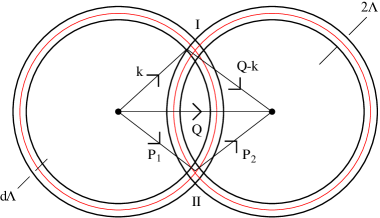
Figure 2: Configuration of momenta near Fermi surface with shell width $2\Lambda$.

References

- [1] Pei-Ming Ho, Yong-Shi Wu, “Noncommutative Geometry and D-branes”, Phys. Lett. B398 (1997) 52; [hep=th/9611233].
- [2] Miao Li, “Strings from IIB Matrices”, Nucl. Phys. B499 (1997) 149; [hep-th/9612222].
- [3] A. Connes, M. R. Douglas, Albert Schwarz, “Noncommutative Geometry and Matrix Theory: Compactification on Tori”, JHEP 9802 (1998) 003; [hep-th/9711162].
- [4] N. Seiberg, E. Witten, “String Theory and Noncommutative Geometry”, JHEP 9909:032 (1999); [hep-th/9908142].
- [5] M. R. Douglas, N. A. Nekrasov, “Noncommutative Field Theory”, Rev. Mod. Phys. 73 (2002) 977; [hep-th/0106048].
- [6] R. J. Szabo, “Quantum Field Theory on Noncommutative Spaces”, Phys. Rept. 378 (2003) 207; [hep-th/0109162].
- [7] M. Li and Y.-S. Wu, Physics in Noncommutative World. Vol. 1: Field Theories, Princeton, USA: Rinton Press (2002) 596 p.
- [8] L. Alvarez-Gaume, M.A. Vazquez-Mozo, “General Properties of Noncommutative Field Theory”, Nucl. Phys. B 668 293-321 (2003); [hep-th/0305093].
- [9] S. Minwalla, M. Van Raamsdonk, N. Seiberg, “Noncommutative Perturbative Dynamics”, JHEP 0002:020 (2000), [hep-th/9912072].
- [10] P. Nozières, Theory of Interacting Fermi Systems, W. A. Benjamin, inc., 1964.
- [11] A. A. Abrikosov, L. P. Gorkov, I. E. Dzyaloshinski, Quantum Field Theoretical Methods in Statistical Physics, Pergamon Press, 1965.
- [12] D. Pines, P. Nozières, The Theory of Quantum Liquids V. I, W. A. Benjamin, inc., 1966.
- [13] E. M. Lifshitz, L. P. Pitaevskii, Statistical Physics, part 2, Pergamon press, Oxford, 1986.
- [14] V. N. Popov, Functional Integrals in Quantum Field Theory and Statistical Physics, D. Reidel Publishing Company, 1983.
- [15] G. Benfatto, G. Gallavotti, “Perturbation Theory of the Fermi Surface in a Quantum Liquid. A General Quasiparticle Formalism and One-Dimensional System”, J. of Stat. Phys. 59 (1990) 541; “Renormalization-Group Approach to Theory of Fermi Surface”, Phys. Rev. B 42 (1990), 9967.
- [16] J. Polchinski, “Effective Field Theory on the Fermi Surface”, Proccedings of 1992 Theoretical Advanced Study Institute in Elementary Particle Physics, eds. J. Harvey and J. Polchinski (World Scientific, Singapore, 1993) [hep-th/9210046].
- [17] R. Shankar, “Renormalization-Group Approach to Interacting Fermions”, Rev. Mod. Phys. 66 1 (1994), 129.
- [18] T. Chen, J. Frölich, M. Steifert, “Renormalization Group Methods: Landau-Fermi Liquid and BCS Superconductor”, [cond-mat/9508063].
- [19] N. Dupuis, “Fermi Liquid Theory; a Renormalization Group Approach”, Eur. Phys. J. B 3, (1998), 315; “Renormalization-Group Approach to Fermi-Liquid Theory”, Phys. Rev. B 54, (1996), 3040.
- [20] D. Belitz, T. R. Kirkpatrik, “Theory of Many-Fermion System”, Phys Rev B 56 (1997), 6513.
- [21] Xiao-Gang Wen, Quantum Field Theory of Many Body Systems, Oxford University Press (2004).
- [22] J. K. Jain, P. W. Anderson, Beyond the Fermi Liquid Paradigm: Hidden Fermi Liquids, Proc. Natl. Acad. Sci. (U.S.A) 106, (2009) 9131.
- [23] P. Horava and C. A. Keeler, JHEP 0707, 059 (2007) [arXiv:hep-th/0508024].
- [24] P. Horava, “Stability of Fermi Surfaces and K-theory”, Phys. Rev. Lett. 95 016405 (2005).
- [25] S. J. Rey, Prog. Theor. Phys. Suppl. 177, 128 (2009) [arXiv:0911.5295 [hep-th]].
- [26] D. Bak and S. J. Rey, JHEP 1009, 032 (2010) [arXiv:0912.0939 [hep-th]].
- [27] S. S. Lee, Phys. Rev. D 79, 086006 (2009) [arXiv:0809.3402 [hep-th]].
- [28] M. Berkooz and D. Reichmann, JHEP 0810, 084 (2008) [arXiv:0807.0559 [hep-th]].
- [29] M. Kulaxizi and A. Parnachev, Phys. Rev. D 78, 086004 (2008) [arXiv:0808.3953 [hep-th]].
- [30] S. Sachdev, arXiv:1006.3794 [hep-th].
- [31] N. Read, Phys. Rev. B 58, 16262 (1998) [arXiv:cond-mat/9804294].
- [32] R. Jackiw, “Physical Instances of Noncommuting Coordinates”, Nucl. Phys. Proc. Suppl. B 108, (2002) 30, [hep-th/010057].
- [33] J. L. F. Barbon and A. Paredes, “Noncommutative Field Theory and the Dynamics of Quantum Hall Fluids,” Int. J. Mod. Phys. A 17, 3589 (2002) [arXiv:hep-th/0112185].
- [34] K. Landsteiner, “Quasiparticles in Non-commutative Field Theory”, [hep-th/0011003].
- [35] G-H. Chen, Y.-S. Wu, “Renormalization Group Equations and the Lifshitz Point in Noncommutative Landau-Ginsburg Theory”, Nucl. Phys. B 622, 189 (2002), [hep-th/0110134].
- [36] D. Bak, S. K. Kim, K. -S. Soh, J. H. Yee, “Exact Wave Functions in a Noncommutative Field Theories”, Phys. Rev. Lett. 85, 3087 (2000).
- [37] J. Gomis, K. Landsteiner, E. Lopez, “Nonrelativistic Noncommutative Field Theory on UV/IR Mixing”, Phys. Rev. D 62, 105006 (2000).
- [38] T. Mateos, A. Moreno, “A Note on Unitarity of Nonrelativistic Noncommuative Theories”, Phys. Rev. D 64, 047703 (2001).
- [39] D. Bak, S. K. Kim, K. -S. Soh, J. H. Yee, “Noncommutative Fermionic Field Theories with Smooth Commutative Limit”, Phys. Rev. D 63, 047701, (2001).
- [40] J.L.F. Barbon, D. Gerber, “A Note on the Topological Order in Noncommutative Hall Fluids”, Int. J. Mod. Phys. A 22, 5287 (2007).
- [41] E. T. Akhmedov, P. DeBoer and G. W. Semenoff, JHEP 0106, 009 (2001) [arXiv:hep-th/0103199].
- [42] K.S. Moon, V. Pasquier, C. Rim, J. Yeo “Non-commutative field theory approach to two-dimensional vortex liquid system,” arXiv:cond-mat/0302282.
- [43] P. Castorina, G. Riccobene, and D. Zappalà “Inhomogeneous chirial symmetry breaking in noncommutative four-fermion interactions”, Phys. Rev. D69, 105024, (2004).
- [44] I. Y. Aref’eva, D. M. Belov, and A.S. Koshelev, “A Note on UV/IR for Noncommutative Complex Scalar Field,” arXiv:hep-th/0001215.
- [45] J. Zinn-Justin, “Quantum Field Theory and Critical Phenomena,” Oxford University Press, (2002).