The Origin and Evolution of the Halo PN BoBn 1:
From a Viewpoint of Chemical Abundances Based on Multiwavelength Spectra

Abstract

We have performed a comprehensive chemical abundance analysis of the extremely metal-poor ([Ar/H]$<$–2) halo planetary nebula (PN) BoBn 1 based on IUE archive data, Subaru/HDS spectra, VLT/UVES archive data, and Spitzer/IRS spectra. We have detected over 600 lines in total and calculated ionic and elemental abundances of 13 elements using detected optical recombination lines (ORLs) and collisionally excited lines (CELs). The estimations of C, N, O, and Ne abundances from the ORLs and Kr, Xe, and Ba from the CELs are done the first for this nebula, empirically and theoretically. The C, N, O, and Ne abundances from ORLs are systematically larger than those from CELs. The abundance discrepancies apart from O could be explained by a temperature fluctuation model, and that of O might be by a hydrogen deficient cold component model. We have detected 5 fluorine and several slow neutron capture elements (the s-process). The amounts of [F/H], [Kr/H], and [Xe/H] suggest that BoBn 1 is the most F-rich among F detected PNe and is a heavy s-process element rich PN. We have confirmed dust in the nebula that is composed of amorphous carbon and PAHs with a total mass of 5.8$\times$10^-6 $M_{\odot}$. The photo-ionization models built with non-LTE theoretical stellar atmospheres indicate that the progenitor was a 1-1.5 $M_{\odot}$ star that would evolve into a white dwarf with an $\sim$0.62 $M_{\odot}$ core mass and $\sim$0.09 $M_{\odot}$ ionized nebula. We have measured a heliocentric radial velocity of +191.6 $\pm$1.3 km s^-1 and expansion velocity 2$V_{\rm exp}$ of 40.5 $\pm$ 3.3 km s^-1 from an average over 300 lines. The derived elemental abundances have been reviewed from the standpoint of theoretical nucleosynthesis models. It is likely that the elemental abundances except N could be explained either by a 1.5 $M_{\odot}$ single star model or by a binary model composed of 0.75 $M_{\odot}$ + 1.5 $M_{\odot}$ stars. Careful examination implies that BoBn 1 has evolved from a 0.75 $M_{\odot}$ + 1.5 $M_{\odot}$ binary and experienced coalescence during the evolution to become a visible PN, similar to the other extremely metal-poor halo PN, K 648 in M 15.

1. Introduction

Planetary Nebulae (PNe) represent a stage in the evolution of low- to intermediate-mass stars with initial masses of 1-8 $M_{\odot}$. At the end of their life, a star of such mass evolves first into a red giant branch (RGB) star, then an asymptotic giant branch (AGB) star, next a PN, and finally a white dwarf. During their evolution, such stars eject a large amount of their mass. The investigation of chemical abundances in PNe enables the determination of how much of a progenitor’s mass becomes a PN, when and how elements synthesized in the progenitor were brought to the surface, and how chemically rich the Galaxy was when the progenitors were born.

Currently, over 1,000 objects are regarded as PNe in the Galaxy (Acker et al. 1991). Of these, about 14 objects have been identified as halo members from their location and kinematics since the PN K 648 was discovered in M 15 (Pease 1928). Halo PNe are interesting objects as they provide direct insight into the final evolution of old, low-mass halo stars, and they are able to convey important information for the study of low-mass star evolution and the early chemical conditions of the Galaxy. However, in extremely metal-poor and C- and N-rich ([C,N/O]$\gtrsim$0, [Ar/H]$<$–2) halo PNe, there are unresolved issues on chemical abundances and evolution time scales. BoBn 1 (PN G108.4–76.1) is one of the C- and N-rich and extremely metal-poor halo PNe ([C, N/O]$>$1, [Ar/H]=–2.22$\pm$0.09, [Fe/H]=–2.39$\pm$0.14; this work), which composes a class of PN together with K 648 (Otsuka 2007, see Table 20) and H 4-1 (Otsuka et al. 2003).

The progenitors of halo PNe are generally thought to be $\sim$0.8 $M_{\odot}$ stars, which is the typical mass of a halo star. Above mentioned three metal-poor C- and N-rich halo PNe, however, show signatures that they have evolved from massive progenitors. For example, they would become N-rich, but would not C-rich if they have evolved from $\sim$0.8 $M_{\odot}$ single stars with [Fe/H]$\sim$–2.3 ($Z$=10^-4), according to the current stellar evolution models (e.g., Fujimoto et al. 2000). To become C-rich PNe, the third dredge-up (TDU) must take place in the late AGB phase. The efficiency of the TDU depends on the initial mass and composition, with increasing efficiency in models of increasing mass, or decreasing metallicity. At halo metallicities, it is predicted that the TDU is efficient in stars with initial masses greater than $\sim$1 $M_{\odot}$ (Karakas 2010; Stancliffe 2010). Also, current stellar evolutionary models predict that the post-AGB evolution of a star with an initial mass $\sim$0.8 $M_{\odot}$ proceeds too slowly for a visible PN to be formed. The origin and evolution of halo PNe are still one of the unresolved big problems in this research field.

How did these progenitor stars become visible C- and N-rich halo PNe? To answer this key question would deepen understanding of low-mass star evolution, in particular, extremely metal-poor C-rich stars found in the Galactic halo, and Galactic chemical evolution at early phases. If we can accurately estimate elemental abundances and ejected masses, then we can directly estimate elemental yields synthesized by PNe progenitors which might provide a constraint to the growth-rate of core mass, the number of thermal pulses and dredge-up mass. Hence we can build realistic stellar evolution models and Galactic chemical evolution models. We have observed these extremely metal-poor C- and N-rich halo PNe using the Subaru/High-Dispersion Spectrograph (HDS) and we also utilized collecting archival data carefully in order to revise our picture of these objects. In this paper, we focus on BoBn 1.

The known nebular and stellar parameters of BoBn 1 are listed in Table 1. Zijlstra et al. (2006) have associated BoBn 1 with the leading tail of the Sagittarius (Sgr) Dwarf Spheroidal Galaxy, which traces several halo globular clusters. The heliocentric distance to the Sgr dwarf Galaxy is $\sim$24.8 kpc (Kunder & Chaboyer 2009), while the distance to this object is between 16.5 (Henry et al. 2004) and 29 kpc (Kingsburgh & Barlow 1992).

BoBn 1 is a unique PN in that it might possess information about the chemical building-up history of the Galactic halo. Otsuka et al. (2008a) found that the [C/Fe] and [N/Fe] abundances of BoBn 1 are compatible with those of carbon-enhanced metal-poor (CEMP) stars. The C and N overabundances of CEMP can be explained by theoretical binary interaction models (e.g., Komiya et al. 2007; Lau et al. 2007). Otsuka et al. (2008a) detected two fluorine (F) lines and found that BoBn 1 is the most F-enhanced and metal-poor PN among F-detected PNe. They found that the C, N, and F overabundances of BoBn1 are comparable to those of the CEMP star HE1305+0132 (Schuler et al. 2007). Through a comparison between the observed enhancements of C, N, and F with the theoretical binary nucleosynthesis model by Lugaro et al. (2008), they concluded that BoBn 1 might share its origin and evolution with CEMP-s stars such as HE1305+0132, and if that is the case the slow neutron capture process (the s-process) should be considered.

According to current evolutionary models of low- to intermediate-mass stars, the s-process elements are synthesized by slowly capturing neutrons during the thermal pulse AGB phase. The s-process elements together with carbon are brought to the stellar surface by the TDU. If we could find signatures that BoBn 1 has experienced binary evolutions such as mass transfer from a massive companion and coalescence, the issues on chemical abundances and evolutionary time scale would be simultaneously resolved. It would also be of great significance to reveal the origin of these elements in the early Galaxy through the study of metal-poor objects such as BoBn 1. We will search s-process elements and investigate their enhancement in BoBn 1.

In this paper, we present a chemical abundance analysis of BoBn 1 using the newly obtained Subaru/HDS spectra, ESO VLT/UVES, Spitzer/IRS and IUE archive data. We detect several candidate collisional excited lines (CELs) of s-process elements and optical recombination lines (ORLs) of N, O, and Ne. We determine ionic and chemical abundances of 13 elements using ORLs and CELs. We construct a detailed photo-ionization model to derive the properties of the central star, ionized nebula, and dust. We also check consistency between our abundance estimations and the model. Finally, we compare the empirically derived abundances with the theoretical nucleosynthesis model values and discuss evolutionary scenarios for BoBn 1.

Table 1Nebular and Stellar Parameters of BoBn 1

Quantity	Value	References
Name	BoBn 1 (PN G108.4–76.1)	discovered by Boeshaar & Bond (1977)
Position (J2000.0)	$\alpha$=00:37:16.03 $\delta$=–13:42:58.48
Distance (kpc)	22.5;29	Hawley & Miller (1978);Kingsburgh & Barlow (1992)
	18.2;16.5	Mal’kov (1997);Henry et al. (2004)
	24.8	Kunder & Chaboyer (2009)
Size (arcsec)	$\sim$2 (diameter)	This work (see Fig. 1)
$\log F(\rm H\beta)$ (erg cm-2 s-1)	–12.54;–12.43	Cuisinier et al. (1996);Wright et al. (2005)
	–12.38;–12.53(observed);–12.44(de-redden)	Kwitter et al. (2003);This work;This work
$c(\rm H\beta)$	0.18;0.0;0.09	Cahn et al. (1992);Kwitter et al. (2003);This work
Rad. Velocity (km s-1)	191.6 (heliocentric)	This work
Exp. Velocity ($2V_{\rm exp}$)	See Table 6	This work
$T_{\epsilon}$ (K)	See Table 8	This work
$n_{\epsilon}$ (cm-3)	See Table 8	This work
Abundances	See Table 19	therein Table 19
$\log\,(L_{\star}/L_{\odot})$	3.57;3.72;3.07	Mal’kov (1997);Zijlstra et al. (2006);This work
$\log\,g$ (cm s-2)	5.52;6.5	Mal’kov (1997);This work
$M_{\star}$ (M⊙)	0.575;0.62	Mal’kov (1997);This work
$T_{\star}$ (K)	125 000;96 300	Howard et al. (1997);Mal’kov (1997)
	125 260	This work
Magnitude	16(B),14.6(R),16.13(J),15.62(H),15.18(K)	Simbad data base

2. Data & Reductions

2.1. Subaru/HDS observations

The spectra of BoBn 1 were taken using the High-Dispersion Spectrograph (HDS; Noguchi et al. 2002) attached to one of the two Nasmyth foci of the 8.2-m Subaru telescope atop Mauna Kea, Hawaii on October 6th 2008 (program ID: S08B-110, PI: M.Otsuka). In Fig. 1, we present the optical image of BoBn 1 taken by the HDS silt viewer camera ($\sim 0.^{\prime\prime}12$ pixel^-1, no filters) during the HDS observation. The sky condition was clear and stable, and the seeing was between $0.^{\prime\prime}4$ and $0.^{\prime\prime}6$. The FWHM of the image is $\sim$1^′′. BoBn 1 shows a small protrusion toward the southeast.

Spectra were taken for two wavelength ranges, 3600-5400 Å (hereafter, the blue region spectra) and 4600-7500 Å (the red region spectra). An atmospheric dispersion corrector (ADC) was used to minimize the differential atmospheric dispersion through the broad wavelength region. In these spectra, there are many recombination lines of hydrogen, helium, & metals and collisionally excited lines (CELs). These numerous spectral lines allowed us to derive reliable chemical compositions. We used a slit width of $1.^{\prime\prime}2$ (0.6 mm) and a 2$\times$2 on-chip binning, which enabled us to achieve a nominal spectral resolving power of $R$=30 000 with a 4.3 binned pixel sampling. The slit length was set to avoid overlap of the echelle diffraction orders at the shortest wavelength portion of the observing wavelength range in each setup. This corresponds to $8^{\prime\prime}$ (4.0mm), in which the nebula fits well and can allow us to directly subtract sky background from the object frames. The CCD sampling pitch along the slit length projected on the sky is $\sim 0.^{\prime\prime}276$ per binned pixel. The achieved S/N is $>$40 at the nebular continuum level even in both ends of each Echelle order. The resulting resolving power is around $R$ $>$33 000, which derived from the mean of the full width at half maximum (FWHM) of narrow Th-Ar and night sky lines. All the data were taken as a series of 1800 sec exposure for weak emission-lines and 300 sec exposures for strong emission-lines. The total exposure times were 16 200 sec for red region spectra and 7200 sec for blue region spectra. During the observation, we took several bias, instrumental flat lamp, and Th-Ar comparison lamp frames, which were necessary for data reduction. For the flux calibration, blaze function correction, and airmass correction, we observed a standard star HR9087 at three different airmass.

2.2. VLT/UVES archive data

We also used archival high-dispersion spectra of BoBn 1, which are available from the European Southern Observatory (ESO) archive. These spectra were observed on August 2002 (program ID: 069.D-0413, PI: M.Perinotto) and June 2007 (program ID: 079.D-0788, PI: A.Zijlstra), using the Ultraviolet Visual Echelle Spectrograph (UVES; Dekker et al. 2000) at the Nasmyth B focus of KUEYEN, the second of the four 8.2-m telescopes of the ESO Very Large Telescope (VLT) at Paranal, Chile. We call the August 2002 data “UVES1” and the June 2007 data “UVES2” hereafter. We used these data to compensate for unobserved spectral regions and order gaps in the HDS spectra. We normalized these data to the HDS spectra using the intensities of detected lines in the overlapped regions between HDS and UVES1 & 2.

These archive spectra covered the wavelength range of 3300-6600 Å in UVES1 and 3300-9500 Å in UVES2. The entrance slit size in both observations was 11^′′ in length and 1$.^{\prime\prime}5$ in width, giving $R$ $>$30 000 derived from Th-Ar and sky lines. The CCDs used in UVES have 15 $\mu$m pixel sizes. For UVES1 an 1$\times$1 binning CCD pattern was chosen. For UVES2 a 2$\times$2 on-chip binning pattern was chosen. The sampling pitch along the wavelength dispersion was $\sim$0.015-0.02 Å pixel^-1 for UVES1 and $\sim$0.03-0.04 Å pixel^-1 for UVES2. The exposure time for UVES1 was 2700 sec $\times$ 4 frames, 10 800 sec in total. The exposure time for UVES2 was 1500 sec $\times$ 2 frames, 3000 sec in total. The standard star Feige 110 was observed for flux calibration.

In Fig. 2, we present the combined HDS and UVES spectrum of BoBn 1 normalized to the H$\beta$ flux. The spectrum for the wavelength region of 3650-7500 Å is from the HDS data and that of 3450-3650 Å & $>$7500 Å is from the UVES data.

The observation logs are summarized in Table 2. The detected lines in the Subaru/HDS and VLT/UVES spectra are listed in Appendix A.

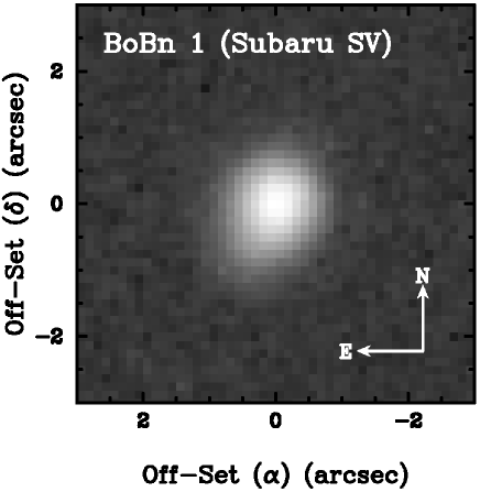
Figure 1.— The optical image of BoBn 1 taken by the Subaru/HDS silt viewer camera. The seeing was 0.4^′′ when we took this image and the nebular FWHM was measured to $\sim$1^′′.

Figure 2.— The spectrum of BoBn 1. The flux density is normalized so that H$\beta$ flux $F(H\beta)$ = 100.

Table 2Journal of the HDS and UVES observations.

Instr.	Obs.Date	seeing	Range	binning	Exp.
		(′′)	(Å)		(sec)
HDS	2008/10/06	0.4-0.6	3650-5400	2$\times$2	1800$\times$4
		0.4-0.6	3650-5400	2$\times$2	600$\times$3
		0.4-0.6	4600-7500	2$\times$2	1800$\times$9
		0.4-0.6	4600-7500	2$\times$2	600$\times$3
UVES	2002/08/04	0.8-1.5	3300-6600	1$\times$1	2700$\times$4
	2007/06/30	0.5-0.7	3300-9500	2$\times$2	1500$\times$2

2.3. IUE archive data

We complemented optical spectra with UV spectra obtained by the International Ultraviolet Explorer (IUE) to derive C⁺, C²⁺, N²⁺, and N³⁺ abundances from semi-forbidden lines C ii], C iii], N iii], and N iv], since these emission lines cannot be observed in the optical region. These IUE spectra were retrieved from the Multi-mission Archive at the STScI (MAST). We collected the high- and low-resolution IUE spectra taken by the Short Wavelength Prime (SWP) and Long Wavelength Prime/Long Wavelength Redundant (LWP/LWR) cameras. Our used data set is listed in Table 3, and the wavelength dispersion mode is indicated in the column 3. All the IUE observations were made using the large aperture (10.3$\times$23 arcsec²). SWP and LWP/LWR spectra cover the wavelength range of 1150-1980 Å and 1850-3350 Å, respectively. For each SWP and LWP/LWR spectra, we did median combine to improve the S/N. The combined short wavelength spectrum was used to measure fluxes of emission-lines in $\lesssim$1910 Å because this allowed us to separate C iii$]$$\lambda$1906/08 and C iv $\lambda$1548/51 lines. C iii$]$$\lambda$1906/08 are important as a density diagnostic. The combined long wavelength spectrum was for measurements of emission-line fluxes in $\gtrsim$2000 Å. The measured line fluxes were normalized to the H$\beta$ flux using theoretical ratios of He ii $I$($\lambda$1640)/($\lambda$4686) for the short wavelength spectrum and $I$($\lambda$2512)/($\lambda$4686) for the long wavelength spectrum, respectively, adopting an electron temperature $T_{\epsilon}$ = 8840 K and density $n_{\epsilon}$ = 10⁴ cm^-3 as given by Storey & Hummer (1995), then normalized to the H$\beta$ flux. The interstellar extinction correction was made using equation (1) (see section 3.1). The observed and normalized fluxes of detected lines are listed in the columns 4 and 5 of Table 4, respectively.

Table 3Journal of IUE observations.

Camera	Data ID.	disp.	Range	Obs.Date	Exp.time
			(Å)		(sec)
LWR	16515	low	1850-3350	1983-08-03	6780
LWP	23692	low	1850-3350	1992-08-13	1500
LWP	23697	low	1850-3350	1992-08-14	7200
LWP	23699	low	1850-3350	1992-08-15	12 000
SWP	45367	high	1150-1980	1992-08-18	7200
LWP	23713	low	1850-3350	1992-08-18	1800
SWP	45369	high	1150-1980	1992-08-18	10 500
SWP	45371	high	1150-1980	1992-08-19	19 800
SWP	45386	high	1150-1980	1992-08-21	9000

2.4. Spitzer archive data

We used two data sets (program IDs: P30333 PI: A.Zijlstra; P30652 PI: J.Bernard-Salas) taken by the Spitzer space telescope in December 2006. The data were taken by the Infrared Spectrograph (IRS, Houck et al. 2004) with the SH (9.5-19.5 $\mu$m), LH (5.4-37$\mu$m), SL (5.2-14.5 $\mu$m) and LL (14-38$\mu$m) modules. In Fig. 3 we present the Spitzer spectra of BoBn 1. We downloaded these data using Leopard provided by the Spitzer Science Center. The one-dimensional spectra were extracted using Spice version c15.0A. We extracted a region within $\pm$1^′′ from the center of each spectral order summed up along the spatial direction. For SH and LH spectra, we subtracted sky background using off-set spectra. We normalized the SL and LL data to the SH and LH using the measured fluxes of [S iv] $\lambda$10.5$\mu$m, H i $\lambda$12.4 $\mu$m, [Ne ii] $\lambda$12.8$\mu$m, [Ne iii] $\lambda$15.6$\mu$m, and [Ne iii] $\lambda$36.0$\mu$m. Finally, the measured line fluxes were normalized to the H$\beta$ flux. The observed line ratio H i $I$(11.2$\mu$m)/$I$($\lambda$4861) (3.1$\times$10^-3) is consistent with the theoretical value (3.15$\times$10^-3) for $T_{\epsilon}$ = 8840 K and $n_{\epsilon}$ = 10⁴ cm^-3 as given by Storey & Hummer (1995). We did not therefore perform interstellar extinction correction.

The observed and normalized fluxes of detected lines are listed in Table 5. In addition to the ionized gas emissions, the amorphous carbon dust continuum and the polycyclic aromatic hydrocarbons (PAHs) feature around 6.2, 7.7, 8.7, and 11.2 $\mu$m are found for the first time. In Fig. 4, we present these PAH features. The 11.2 $\mu$m emission line is a complex of the narrow width H i 11.2 $\mu$m and the broad PAH 11.2 $\mu$m. The 6.2, 7.7, and 8.7 $\mu$m bands emit strongly in ionized PAHs, while the 11.2 $\mu$m does in neutral PAHs (Bernard-Salas et al. 2009). According to the PAH line profile classifications by Peeters et al. (2002) and van Diedenhoven et al. (2004), BoBn 1’s PAH line-profiles belong to class B. Bernard-Salas et al. (2009) classified 10 of 14 Magellanic Clouds (MCs) PNe into class B based on Spitzer spectra. In measuring PAH band fluxes, we used local continuum subtracted spectrum by a spline function fitting. We followed Bernard-Salas et al. (2009) and measured integrated fluxes between 6.1 and 6.6 $\mu$m for the 6.2 $\mu$m PAH band, 7.2-8.3 $\mu$m for the 7.7 $\mu$m PAH, 8.3-8.9 $\mu$m for the 8.6 $\mu$m PAH, and 11.1-11.7 $\mu$m for the 11.2 $\mu$m. The observed PAH flux ratios $I$(6.2$\mu$m)/$I$(11.2$\mu$m) and $I$(7.7$\mu$m)/$I$(11.2$\mu$m) follow a correlation among MCs PNe, shown in Fig. 2 of Bernard-Salas et al. (2009). BoBn 1 has a hot central star ($>$10⁵ K), so that ionized PAH might be dominant. However, these line ratios of BoBn 1 are somewhat lower than those of excited MCs PNe. One must take a look at a part of the neutral PAH emissions in a photodissociation region (PDR), too.

We found a plateau between 10 and 14 $\mu$m, which are believed to be related to PAH clusters (Bernard-Salas et al. 2009). Meanwhile, MgS feature around 30 $\mu$m sometimes observed in C-rich PNe, was unseen in BoBn 1.

Figure 3.— The Spitzer spectra of BoBn 1 obtained by the SH and LH (upper panel) and the SL and LL modules (lower panel).

Figure 4.— The 6-11$\mu$m PAHs profiles. The PAHs 6.2, 7.9, and 8.7 $\mu$m profile classification (A, B, and C) of Peeters et al. (2002) and the 11.2 $\mu$m classification of van Diedenhoven et al. (2004) are given.

2.5. Data reduction

Data reduction and emission line analysis were performed mainly with a long-slit reduction package noao.twodspec in IRAF. Data reduction was performed in a standard manner.

First, we made a zero-intensity level correction to all frames including flat lamp, object, and Th-Ar comparison frames using the overscan region of each frame and the mean bias frames. We also removed cosmic ray events and hot pixels from the object frames. Second, we trimmed the overscan region and removed scattered light from the flat lamp and object frames. Third, we made a CCD sensitivity correction to the object frames using the median flat frames. Fourth, we extracted a two-dimensional spectrum from each echelle diffraction order of each object frame and made a wavelength calibration using at least two Th-Ar frames taken before and after the object frame. We referred to the Subaru/HDS comparison atlas and a Th-Ar atlas. For the wavelength calibration, we fitted the wavelength dispersion against the pixel number with a fourth- or fifth-order polynomial function. With this order, any systematic trend did not show up in the residuals and the fitting appears to be satisfactory. We also made a distortion correction along the slit length direction using the mean Th-Ar spectrum as a reference. We fitted the slit image in the Th-Ar spectrum with a two-dimensional function. For the HDS spectra, we adopted fourth- and third-order polynomial functions for the wavelength and space directions, respectively. The fitting residual was of the order of 10^-4 Å. For the UVES spectra, we adopted third- and second-order polynomial functions for the wavelength and space directions, respectively. The fitting residual was of the order of 10^-3 Å. Fifth, we determined a sensitivity function using sky-subtracted standard star frames and obtained sky-subtracted and flux-calibrated two-dimensional PN spectra. The probable error in the flux calibration was estimated to be less than 5 ${\%}$. Finally, we made a spatially integrated one-dimensional spectrum, and we combined all the observed echelle orders using IRAF task scombine.

In measuring emission line fluxes, we assumed that the line profiles were all Gaussian and we applied multiple Gaussian fitting techniques.

3. Results

Table 4The detected lines in the IUE spectra.

$\lambda_{\rm lab.}$	Ion	$f$($\lambda$)	$F$($\lambda$)	$I$($\lambda$)
(Å)			(erg s-1 cm-2)	$[$$I$(H$\beta$)=100$]$
1485	N iv]	1.306	1.41(–13) $\pm$ 5.47(–14)	45.81 $\pm$ 17.84
1548	C iv	1.239	3.27(–12) $\pm$ 5.04(–14)	1052.6 $\pm$ 20.22
1551	C iv	1.237	1.62(–12) $\pm$ 4.27(–14)	519.3 $\pm$ 14.96
1640	He ii	1.177	5.13(–13) $\pm$ 7.40(–14)	162.97 $\pm$ 23.57
1750	N iii]	1.154	1.52(–13) $\pm$ 4.16(–14)	48.06 $\pm$ 13.16
1906	C iii]	1.255	2.60(–12) $\pm$ 2.50(–14)	838.88 $\pm$ 12.65
1908	C iii]	1.258	1.87(–12) $\pm$ 2.33(–14)	602.72 $\pm$ 10.28
2324	C ii]	1.388	2.87(–13) $\pm$ 3.60(–14)	36.64 $\pm$ 4.63
	+[O iii]
2424	[Ne iv]	1.134	1.41(–13) $\pm$ 1.46(–14)	17.12 $\pm$ 1.78
2512	He ii	0.969	2.66(–14) $\pm$ 1.29(–14)	3.13 $\pm$ 1.52

Table 5The detected lines in the Spitzer spectra.

$\lambda_{\rm lab.}$	Ion	$F$($\lambda$)	$I$($\lambda$)
($\mu$m)		(erg s-1 cm-2)	$[$$I$(H$\beta$)=100$]$
6.2	PAH	2.62(–14) $\pm$ 1.52(–15)	7.22 $\pm$ 1.35
7.7	PAH	8.13(–14) $\pm$ 2.31(–15)	22.39 $\pm$ 4.04
8.6	PAH	2.02(–14) $\pm$ 1.23(–15)	5.57 $\pm$ 1.05
10.5	$[$S iv$]$	7.36(–15) $\pm$ 1.93(–16)	1.92 $\pm$ 0.05
11.3	H i	1.18(–15) $\pm$ 1.81(–16)	0.31 $\pm$ 0.05
11.3	PAH	4.97(–14) $\pm$ 9.65(–15)	13.68 $\pm$ 3.61
12.4	H i	3.89(–15) $\pm$ 3.01(–16)	1.02 $\pm$ 0.08
12.5	He i	1.72(–15) $\pm$ 4.17(–16)	0.45 $\pm$ 0.11
12.8	$[$Ne ii$]$	9.53(–15) $\pm$ 3.13(–16)	2.49 $\pm$ 0.08
14.6	He i	5.85(–16) $\pm$ 2.40(–16)	0.15 $\pm$ 0.06
15.6	$[$Ne iii$]$	6.17(–13) $\pm$ 4.98(–15)	161.13 $\pm$ 1.30
16.4	He i	2.19(–15) $\pm$ 2.65(–16)	0.57 $\pm$ 0.07
18.7	$[$S iii$]$	2.65(–15) $\pm$ 1.79(–16)	0.69 $\pm$ 0.05
19.1	H i	1.14(–15) $\pm$ 2.64(–16)	0.30 $\pm$ 0.07
25.9	$[$O iv$]$	4.77(–14) $\pm$ 5.20(–16)	12.46 $\pm$ 0.14
36.0	$[$Ne iii$]$	5.10(–14) $\pm$ 7.04(–15)	13.32 $\pm$ 1.84

3.1. Interstellar reddening correction

We have detected over 600 emission lines in total. Before proceeding to the chemical abundance analysis, it is necessary to correct the spectra for the effects of absorption due to the Earth’s atmosphere and interstellar reddening. The former was performed using experimental functions measured at the Keck observatories and the ESO/VLT. The interstellar reddening correction was made by determining the reddening coefficient at H$\beta$, $c$(H$\beta$). We fitted the observed intensity ratio of H$\alpha$ to H$\beta$ with the theoretical ratios computed by Storey & Hummer (1995). Two different situations are assumed for some lines: Case A assumes that the nebula is transparent to the lines of all series of hydrogen; Case B assumes the nebula is partially opaque to the lines of the Lyman series but is transparent for the Balmer series of hydrogen. Initially, we assumed that $T_{\epsilon}$ = 10⁴ K and $n_{\epsilon}$ = 10⁴ cm^-3 in Case B, and we estimated $c$(H$\beta$) = 0.087 $\pm$ 0.004 from the HDS spectra. That is an intermediate value between Cahn et al. (1992) and Kwitter et al. (2003) (see Table 1). For the UVES spectra, we estimated $c$(H$\beta$) = 0.066 by the same manner. From Seaton’s (1979) relation $c$(H$\beta$) = 1.47$E(B-V)$ one obtains $E(B-V)$ = 0.06 for the HDS spectra and 0.04 for UVES spectra, which are comparable to the Galactic value (0.02) to the direction to BoBn 1 measured by the Galactic extinction model of Schlegel et al. (1998).

All of the line intensities were then de-reddened using the formula:

$$\log_{10}\left[\frac{I(\lambda)}{I{\rm(H\beta)}}\right]=\log_{10}\left[\frac{F(\lambda)}{F{\rm(H\beta)}}\right]+c({\rm H\beta})f(\lambda),$$ (1)

where $I(\lambda)$ is the de-reddened line flux; $F(\lambda)$ is the observed line flux; and $f(\lambda)$ is the interstellar extinction at $\lambda$. We adopted the reddening law of Cardelli et al. (1989) with the standard value of $R_{V}$ = 3.1 for $f(\lambda)$. We observed $F(H\beta)$ = 2.56$\times$10^-13 $\pm$ 2.13$\times$10^-16 erg s^-1 cm^-2 ($X$($-Y$) stands for $X$ $\times$ 10^-Y, hereafter) within the $1.^{\prime\prime}2$ slit in the HDS observation. We estimated captured light from BoBn 1 using the image presented in Fig. 1, to be about 86.8 $\%$ of the light from BoBn 1 in the HDS observation. The intrinsic observed H$\beta$ flux is 2.95(–13) $\pm$ 3.45(–16) erg s^-1 cm^-2 and the de-reddened H$\beta$ flux is 3.63(–13) $\pm$ 6.47(–14) erg s^-1 cm^-2 including the error of $c$(H$\beta$).

3.2. Radial and expansion velocities

We present the line-profiles of selected ions in Fig. 5. The observed wavelength at the time of observation was corrected to the averaged line-of-sight heliocentric radial velocity of +191.60 $\pm$ 1.25 km s^-1 among over 300 lines detected in the HDS spectra. The line-profiles can be represented by a single Gaussian for weak forbidden lines such as [Ne v] $\lambda$3426 and metal recombination lines such as O ii $\lambda$4642. For the others, the profiles can be represented by the sum of two or three Gaussian components.

Most of the detected lines are asymmetric profile, in particular the profiles of low-ionization potential ions show strong asymmetry. The asymmetric line-profiles are sometimes observed in bipolar PNe having an equatorial disk structure. The similar line-profiles are also observed in the halo PN H4-1 (Otsuka et al. 2006). H4-1 has an equatorial disk structure and multi-polar nebulae. The elongated nebular shape of BoBn 1 (Fig. 1) might indicate the presence of such an equatorial disk. The receding ionized gas (especially, low-ionization potential ions) from the observers around the central star would be strongly weakened by the equatorial disk. In contrast, the relatively large extent bipolar flows perpendicular to the equatorial disk might be unaffected by the disk. Due to such a geometry, we observe asymmetric line-profiles.

In Table 6, we present twice the expansion velocity 2$V_{\rm exp}$ measured from selected lines. When we fit line-profile with two or three Gaussian components, we define that 2$V_{\rm exp}$ corresponds to the difference between the positions of the red and blue shifted Gaussian peak components. We call expansion velocity measured by this method ‘2$V_{\rm exp}$(a)’.

When we can fit line-profile with single Gaussian, we determine 2$V_{\rm exp}$ from following equation,

$$2V_{\rm exp}=(V_{\rm FWHM}^{2}-V_{\rm therm}^{2}-V_{\rm instr}^{2})^{1/2},$$ (2)

where $V_{\rm FWHM}$ is the velocity FWHM of each Gaussian component. $V_{\rm therm}$ and $V_{\rm instr}$ ($\sim$9 km s^-1) are the thermal broadening and the instrumental broadening, respectively (Robinson et al. 1982). $V_{\rm therm}$ is represented by 21.4$(T_{4}/A)^{1/2}$, where $T_{4}$ is the electron temperature (in units of 10⁴ K) and $A$ is the atomic weight of the target ion. For CELs, we adopted $T_{4}$ listed in Table 9. For ORLs, we adopted $T_{4}$ = 0.88. We call twice the expansion velocity measured by Equation (2) ‘2$V_{\rm exp}$(b)’. We converted 2$V_{\rm exp}$(a) into 2$V_{\rm exp}$(b) using the relation 2$V_{\rm exp}$(b) = (1.74 $\pm$ 0.12) $\times$ 2$V_{\rm exp}$(a) for 2$V_{\rm exp}$(b) $>$ 16 km s^-1, which can be applied only to BoBn 1. We adopted 2$V_{\rm exp}$(b) as twice the expansion velocities for BoBn 1. The averaged $2V_{\rm exp}$(b) is 40.5 $\pm$ 3.28 km s^-1 among selected lines listed in Table 6 and 33.04 $\pm$ 2.61 km s^-1 among over 300 detected lines in the HDS spectra.

In Fig. 6 we present relation between 2$V_{\rm exp}$(b) and ionization potential (I.P.). When we assume that BoBn 1 has a standard ionized structure (i.e., high I.P. lines are emitted from close regions to the central star and low I.P. lines are from far regions), expansion velocity of BoBn 1 seems to be proportional to the distance from the central star. BoBn 1 might have Hubble type flows. We found that 2$V_{\rm exp}$(b) values from ORLs are slightly smaller than CELs with the same I.P., for example, O ii & [O iii] (35.5 eV) and Ne ii & [Ne iii] (41.0 eV). O ii and Ne ii might be emitted from colder regions than [O iii] and [Ne iii] do.

Figure 5.— The line-profiles of selected ions. Vertical and horizontal axes are scaled flux density and velocity with respect to the systemic radial velocity of +191.60 km s^-1, respectively. All are from the HDS spectra except [Ne v]$\lambda$3426 and [S iii]$\lambda$9069 which are from UVES1 and UVES2, respectively.

Table 6Twice the expansion velocities from selected lines.

Ion	$\lambda_{\rm lab}$	I.P.	$2V_{\rm exp}$(a)	$2V_{\rm exp}$(b)
	(Å)	(eV)	(km s-1)	(km s-1)
$[$Ne v$]$	3425	97.1	$\cdots$	10.0
Ne ii	3694	41.0	$\cdots$	34.4
$[$O ii$]$	3726	13.6	32.0	55.6
$[$Ne iii$]$	3868	41.0	$\cdots$	41.5
$[$F iv$]$	4060	62.7	$\cdots$	15.0
C iii	4187	47.9	$\cdots$	31.9
C ii	4267	24.4	$\cdots$	48.4
N iii	4379	47.5	$\cdots$	40.9
N ii	4442	29.6	$\cdots$	41.8
O ii	4642	35.5	$\cdots$	24.2
He ii	4686	54.4	$\cdots$	26.9
$[$Ar iv$]$	4711	40.7	$\cdots$	32.3
$[$Ne iv$]$	4724	63.5	$\cdots$	8.9
$[$F ii$]$	4798	17.4	$\cdots$	33.3
H$\beta$	4861	13.5	$\cdots$	45.0
$[$Fe iii$]$	4881	16.2	$\cdots$	32.6
$[$O iii$]$	5007	35.5	$\cdots$	42.8
$[$N i$]$	5198	0	35.3	61.3
$[$Cl iii$]$	5517	23.8	$\cdots$	56.3
C iv	5812	64.5	$\cdots$	14.3
$[$F iii$]$	5733	35.0	$\cdots$	48.6
He i	5876	24.6	$\cdots$	32.7
$[$O i$]$	6300	0	48.0	83.3
$[$N ii$]$	6548	14.5	37.7	65.4
$[$S ii$]$	6716	10.4	32.1	55.7
$[$Fe iv$]$	6741	30.7	$\cdots$	53.4
$[$Ar iii$]$	7135	27.6	$\cdots$	48.0
$[$S iii$]$	9069	23.3	$\cdots$	49.7

Figure 6.— Relation between 2$V_{\rm exp}$(b) and ionization potential (I.P.). The filled circles are the values from the CELs and the open circles are from the ORLs.

Table 7Atomic data references for CELs.

Line	transition probabilities $A_{ji}$	collisional strength $\Omega_{ij}$
$[$C i$]$	Froese-Fischer & Saha (1985)	Johnson et al. (1987); Péquignot & Aldrovandi (1976)
$[$C ii$]$	Nussbaumer & Storey (1981); Froese-Fischer (1994)	Blum & Pradhan (1992)
C iii$]$	Wiese et al. (1996)	Berrington et al. (1985)
C iv	Wiese et al. (1996)	Badnell & Pindzola (2000); Martin et al. (1993)
[N i]	Wiese et al. (1996)	Péquignot & Aldrovandi (1976); Dopita et al. (1976)
[N ii]	Wiese et al. (1996)	Lennon & Burke (1994)
N iii$]$	Brage et al. (1995); Froese-Fischer (1983)	Blum & Pradhan (1992)
N iv$]$	Wiese et al. (1996)	Ramsbottom et al. (1994)
[O i]	Wiese et al. (1996)	Bhatia & Kastner (1995)
[O ii]	Wiese et al. (1996)	McLaughlin & Bell (1993); Pradhan (1976)
[O iii]	Wiese et al. (1996)	Lennon & Burke (1994)
[O iv]	Wiese et al. (1996)	Blum & Pradhan (1992)
$[$F ii$]$	Storey & Zeippen (2000); Baluja & Zeippen (1988)	Butler & Zeippen (1994)
$[$F iii$]$	Naqvi (1951)	See Text
$[$F iv$]$	Garstang (1951); Storey & Zeippen (2000)	Lennon & Burke (1994)
$[$Ne ii$]$	Saraph & Tully (1994)	Saraph & Tully (1994)
[Ne iii]	Mendoza (1983); Kaufman & Sugar (1986)	McLaughlin & Bell(2000)
[Ne iv]	Becker et al. (1989); Bhatia & Kastner (1988)	Ramsbottom et al. (1998)
[Ne v]	Kaufman & Sugar (1986); Bhatia & Doschek (1993)	Lennon & Burke (1994)
[S ii]	Verner et al. (1996); Keenan et al. (1993)	Ramsbottom et al. (1996)
[S iii]	Tayal & Gupta (1999)	Froese Fischer et al. (2006)
[S iv]	Johnson et al. (1986); Dufton et al. (1982); Verner et al. (1996)	Dufton et al. (1982)
[Cl iii]	Mendoza & Zippen (1982a); Kaufman & Sugar (1986)	Ramsbottom et al. (2001)
[Cl iv]	Mendoza & Zippen (1982b); Ellis & Martinson (1984)	Galavis et al. (1995)
	Kaufman & Sugar (1986)
[Ar iii]	Mendoza (1983); Kaufman & Sugar (1986)	Galavis et al. (1995)
[Ar iv]	Mendoza & Zippen (1982a); Kaufman & Sugar (1986)	Zeippen et al. (1987)
[Fe iii]	Garstang (1957); Nahar & Pradhan (1996)	Zhang (1996)
[Fe iv]	Froese-Fischer & Rubin (1998); Garstang (1958)	Zhang & Pradhan (1997)
[Kr iv]	Biémont & Hansen (1986)	Schöning (1997)
[Kr v]	Biémont & Hansen (1986)	Schöning (1997)
$[$Rb v$]$	Persson et al. (1984)	$\cdots$
[Xe iii]	Biémont et al. (1995)	Schöning & Butler (1998)
Ba ii	Klose et al. (2002)	Schöning & Butler (1998)

3.3. Plasma diagnostics

3.3.1 CEL diagnostics

We have detected a large number of collisionally excited lines (CEL), useful for estimations of the temperatures ($T_{\epsilon}$) and densities ($n_{\epsilon}$). The electron temperature and density diagnostic lines analyzed here arise from various ions, which have a wide variety of ionization potentials ranging from 0 ([N i] & [O i]) to 63.5 eV ([Ne iv]). We have examined the electron temperature and density structure within the nebula of BoBn 1 using 17 diagnostic line ratios. The [O i], [Ne iii], [Ne iv], [S ii], and [S iii] zone electron temperatures and [N i], C iii] and [Ne iii] zone electron densities are estimated for the first time. Electron temperatures and densities were derived from each diagnostic ratio for each line by solving level populations for a multi-level ($\geqq$ 5 for almost all the ions) atomic model using the collision strengths $\Omega_{ij}$ ($j$$>$$i$) and spontaneous transition probabilities $A_{ji}$ for each ion from the references given in Table 7.

The derived electron temperatures and densities are listed in Table 8. Fig. 7 is the diagnostic diagram that plots the loci of the observed diagnostic line ratios on the $n_{\epsilon}$–$T_{\epsilon}$ plane. This diagram shows that most CELs in BoBn 1 are emitted from $T_{\epsilon}$$\sim$12 000–16 000 K and $\log_{10}$ $n_{\epsilon}$$\sim$3.5 cm^-3 ionized gas.

First, we calculated electron densities assuming a constant electron temperature of 12 800 K. Estimated electron densities range from 1030 ([N i]) to 5740 cm^-3 ([S ii]). Although [S ii] and [O ii] have similar ionization potentials, a large discrepancy between their electron densities is found (see Table 8). Kniazev et al. (2008) and Kwitter et al. (2003) estimated [S ii] electron densities as large as 9600 and 7100 cm^-3, respectively. Stanghellini & Kaler (1989), Copetti & Writzl (2002), and Wang et al. (2004) found that the [S ii] density is systematically larger than the [O ii] density in a large number of samples. The curve yielded by the [S ii]$\lambda$6716/31 ratio in the $n_{\epsilon}$ vs $T_{\epsilon}$ plane indicates higher electron density than critical density of these lines, 1600 $\&$ 4100 cm^-3 at $T_{\epsilon}$ = 12 800 K for $\lambda$6716 and $\lambda$6731, respectively (cf. 5740 cm^-3 in Fig. 7). This density discrepancy is not due to the errors in the [O ii] atomic data. Wang et al. (2004) also found the density discrepancy between [S ii] and [O ii] that might be likely caused by errors in the transition probabilities of [O ii] given by Wiese et al. (1996). In the case of BoBn 1, this possibility can be ruled out because we obtained similar [O ii] electron densities even when with the other transition probabilities. The high [S ii] density might be due to high-density blobs in the outer nebula. This could have contributed to producing the small [S ii]$\lambda$6717/$\lambda$6731 ratio and give rise to an apparently high density. Zhang et al. (2005a) pointed out the possibility that a dynamical plow by the ionization front effects yields large density of [S ii] because the ionization potential of S⁺ is close to the H⁺ edge. Since the estimated upper limit to the [S ii] density is close to the H⁺ density derived from the Balmer decrement (see below), this explanation might be plausible. In BoBn 1, caution is necessary when using the [S ii] electron density.

Next, we calculated the electron temperature. An average electron density of 3370 cm^-3, which excluded the $n_{\epsilon}$([N i]) and $n_{\epsilon}$([S ii]), was adopted when estimating electron temperatures except the $T_{\epsilon}$([O i]). [N i] and [O i] are representative of the very outer part of the nebula and probably do not coexist with most of the other ions. $T_{\epsilon}$([O i]) was, therefore, estimated using $n_{\epsilon}$([N i]).

To obtain the [N ii], [O ii] and [O iii] temperatures it is necessary to subtract the recombination contamination to the [N ii] $\lambda$5755, [O ii] $\lambda\lambda$7320/30, and [O iii] $\lambda$4363 lines, respectively. For [N ii] $\lambda$5755, Liu et al. (2000) estimated the contamination to [N ii] $\lambda$5755, $I_{R}$([N ii]$\lambda$5755) in the range 5000 $\leqq$ $T_{\epsilon}$ $\leqq$ 20 000 K as

$$\frac{I_{R}(\rm[N\,{\sc II}]\lambda 5755)}{I(\rm H\beta)}=3.19\left(\frac{T_{\epsilon}}{10^{4}}\right)^{0.33}\times\frac{\rm N^{2+}}{\rm H^{+}},$$ (3)

where N²⁺/H⁺ is the doubly ionized nitrogen abundance. Adopting the value derived from the ORL analysis (see Section 3.6) and using Equation (3), we estimated $I_{R}$([N ii]$\lambda$5755) $\sim$0.1, which is approximately 7 $\%$ of the observed value. Given the corrected [N ii] $\lambda$5755 intensity, the [N ii] temperature is 12 000 K, which is 400 K lower than that obtained without taking into account the recombination effect.

The same effect also exists for the [O ii] $\lambda\lambda$7320/30 lines. We estimated the recombination contribution using the doubly ionized oxygen abundance derived from O ii lines and the equation of Liu et al. (2000) for these lines in the range 5000 $\leqq$ $T_{\epsilon}$ $\leqq$ 10 000 K,

$$\frac{I_{R}(\rm[O\,{\sc II}]\lambda\lambda 7320/30)}{I(\rm H\beta)}=9.36\left(\frac{T_{\epsilon}}{10^{4}}\right)^{0.44}\times\frac{\rm O^{2+}}{\rm H^{+}}.$$ (4)

Using Equation (4), we estimated a contribution of $\sim$7 $\%$ of the observed value and obtained 12 100 K, lower by 700 K than that without the recombination contribution. For [O iii] $\lambda$4363, we estimated the recombination contribution using the O³⁺ abundance derived from the fine-structure line [O iv] $\lambda$25.9$\mu$m adopting $T_{\epsilon}$([Ne iv]) and $n_{\epsilon}$([Ar iv]) and the equation of Liu et al. (2000). We chose the value from this line because O iii lines could be affected by star light excitation and the abundance derived from them could be erroneous. Assuming the ratio of O³⁺(ORLs)/O³⁺(CELs) = 10, we estimated the recombination contribution to [O iii] $\lambda$4363 less than 1$\%$ of the observed value, which has a negligible effect on the $T_{\epsilon}$([O iii]) derivation.

The electron temperature in BoBn 1 ranges from 9520 ([O i]) to 14 920 K ([Ne iv]). Our estimated electron temperatures except for [O ii] are comparable to those of Kwitter et al. (2003) and Kniazev et al. (2008). Their estimated temperatures are 12 400-13 720 K for [O iii], 11 320-11 700 K for [N ii], and 13 250 K for [Ar iii]. Note that the [O ii] electron temperature of 8000 K of Kwitter et al. (2003) was estimated adopting the [S ii] density of 7100 cm^-3. Our $n_{\epsilon}$–$T_{\epsilon}$ plane predicts that the [O ii] temperature is $\sim$10 000 K when adopting [S ii] density.

The ionic abundances derived from the CELs depend strongly on the electron temperature. In the case of [O iii]$\lambda$5007, for example, only 500 K change makes a difference of over 10$\%$ for O²⁺ abundance. It is therefore essential to find the proper electron temperature for each ionized stage of each ion. To that end, we examined the behavior of the electron temperature and density as a function of I.P. The upper panel of Fig. 8 shows that $T_{\epsilon}$ is increasing proportional to I.P. The observed behavior of $T_{\epsilon}$ is consistent with the schematic picture of stratified physical conditions in ionized nebula, where the electron temperature of ions in the inner part should be hotter than that in the outer part. $n_{\epsilon}$ is simply monotonically increasing up to $\sim$40 eV as I.P., except for [S ii]. The [S ii] might be emitted in high-density blobs in the outer nebula as we mentioned above.

To minimize the estimated error for ionic abundances due to electron temperature, we have assumed a 7-zone model for BoBn 1 by reference to Fig. 8. Adopted $T_{\epsilon}$ and $n_{\epsilon}$ for each ion are presented in Table 9. $T_{\epsilon}$([O i]) and $n_{\epsilon}$([N i]) are adopted for ions in zone 0, which have $<$10 eV. $T_{\epsilon}$([N ii]) and $n_{\epsilon}$([S ii]) are adopted for ions in zone 1 (I.P. $<$ 11.3 eV). $T_{\epsilon}$([N ii]) and $n_{\epsilon}$([O ii]) are for zone 2 (11.3-20 eV). $T_{\epsilon}$([S iii]) and $n_{\epsilon}$(C iii]) are for zone 3 (20-25 eV). For zone 4 (25-41 eV), 5 (41-63.5 eV), and zone 6 ($>$ 63.5 eV), we adopted $n_{\epsilon}$([Ar iv]) and $T_{\epsilon}$([O iii]), the averaged value from $T_{\epsilon}$([O iii]) and $T_{\epsilon}$([Ne iv]), and $T_{\epsilon}$([Ne iv]), respectively.

Figure 7.— Plasma diagnostic diagram. Each curve is labeled with an ID number given in Table 8. For $T_{\epsilon}$([N ii]) and $T_{\epsilon}$([O ii]), we corrected for recombination contributions to [N ii] $\lambda$5755 and [O ii] $\lambda\lambda$7320/30, respectively (see text).

Table 8Plasma diagnostics.

	ID	Diagnostic	Ratio	Result
$T_{\epsilon}$	(1)	[Ne iv] ($\lambda$2422+$\lambda$2425)/($\lambda$4715/16/25/26)	100.78$\pm$10.84	14 920$\pm$810
(K)	(2)	[O iii] ($\lambda$4959+$\lambda$5007)/($\lambda$4363)	85.01$\pm$4.32	13 650$\pm$290
	(3)	[Ar iii] ($\lambda$7135)/($\lambda$5192)	85.70$\pm$35.63	13 330$\pm$3 310
	(4)	[Ne iii] ($\lambda$15.5$\mu$m)/($\lambda$3869+$\lambda$3967)	0.20$\pm$0.01	13 050$\pm$140
	(5)	[Ne iii] ($\lambda$3869+$\lambda$3967)/($\lambda$3344)	333.67$\pm$14.63	12 870$\pm$170
	(6)	[N ii] ($\lambda$6548+$\lambda$6583)/($\lambda$5755)	57.55$\pm$1.77	12 000$\pm$190a
	(7)	[S iii] ($\lambda$9069)/($\lambda$6312)	7.42$\pm$0.53	12 460$\pm$490
	(8)	[O i] ($\lambda$6300+$\lambda$6363)/($\lambda$5577)	68.65$\pm$10.76	9520$\pm$550
	(9)	[O ii] ($\lambda$3726+$\lambda$3729)/($\lambda$7320+$\lambda$7330)	10.47$\pm$0.21	12 100$\pm$180b
	(10)	[S ii] ($\lambda$6716+$\lambda$6731)/($\lambda$4069+$\lambda$4076)	13.84$\pm$5.17	12 420-3590
		Average†		13 050
		He i ($\lambda$7281)/($\lambda$6678)	0.21$\pm$0.01	9430$\pm$310
		He i ($\lambda$7281)/($\lambda$5876)	0.05$\pm$0.01	7340$\pm$110
		He i ($\lambda$6678)/($\lambda$4471)	0.83$\pm$0.02	7400+1070
		He i ($\lambda$6678)/($\lambda$5876)	0.27$\pm$0.01	9920$\pm$310
		Average		8520
		(Balmer Jump)/(H 11)		8840$\pm$210
$n_{\epsilon}$	(11)	[N i] ($\lambda$5198)/($\lambda$5200)	1.43$\pm$0.03	1030$\pm$130
(cm-3)	(12)	[O ii] ($\lambda$3726)/($\lambda$3729)	1.65$\pm$0.03	1510$\pm$60
	(13)	C iii] ($\lambda$1906)/($\lambda$1909)	1.39$\pm$0.03	3590$\pm$1000
	(14)	[Ar iv] ($\lambda$4711)/($\lambda$4740)	1.05$\pm$0.07	3960$\pm$1090
	(15)	[Ne iii] ($\lambda$15.5$\mu$m)/($\lambda$36.0$\mu$m)	12.11$\pm$1.69	4400+9010
	(16)	[S ii] ($\lambda$6716)/($\lambda$6731)	8.57$\pm$0.03	5740$\pm$1 310
		Average†		3370
		Balmer decrement		5000-10 000

Figure 8.— Electron temperature (upper) and density (lower) versus ionization potential. Each value is labeled with an ID number given in Table 8.

Table 9Adopted $T_{\epsilon}$ and $n_{\epsilon}$ for CEL ionic abundance calculations.

Zone	Ions	$T_{\epsilon}$(K)	$n_{\epsilon}$(cm-3)
0	C0,N0,O0,Ba+	9520	1030
1	C+,S+	12 000	5740
2	O+,N+,F+,Fe2+	12 000	1510
3	C2+,Ne+,S2+,Cl2+,Xe2+	12 460	3590
4	N2+,O2+,Ne2+,Ar2+,Ar3+,S3+	13 650	3960
	Cl3+,F2+,Fe3+,Kr3+,Kr4+
5	C3+,N3+,O3+	14 290†	3960
6	Ne3+,Ne4+,F3+	14 920	3960

3.3.2 ORL diagnostics

We detected a large number of optical recombination lines (ORL). C iii,iv, O ii,iii,iv, N ii,iii, and Ne ii are for the first time detected. To calculate ORL abundances, the electron temperature and density derived from ORLs are needed. We estimated the electron temperature using the Balmer discontinuity and He i line ratios, and the electron density using the Balmer decrement. The results are listed in Table 8.

The ratio of the jump of continuum emission at the Balmer limit at 3646Å (BJ) to a given hydrogen emission line depends on the electron temperature. Following Liu et al. (2001), we use this ratio to determine the electron temperature. This temperature, $T_{\epsilon}$(BJ), is used to deduce ionic abundances from ORLs. Defining BJ as $I(3646{\rm{\AA}})-I(3681{\rm{\AA}})$, and taking the emissivities of H i Balmer lines and H i, He i, and He ii continuum emissivities, Liu et al. (2001) gave the following equation:

$$T_{\epsilon}({\rm BJ})=368\left(1+0.259{\rm\frac{N(He^{+})}{N(H^{+})}}+3.409{\rm\frac{N(He^{2+})}{N(H^{+})}}\right)$$ (5)

$$\times\left(\frac{I(3646\,{\rm{\AA}})-I(3681\,{\rm{\AA}})}{I{\rm(H\,11)}}\right)^{-1.5}$$

[$I({\rm 3646\,{\AA}})-I({\rm 3681\,{\AA}})]/I({\rm H\,11})$ is in units of Å^-1. $T_{\epsilon}$(BJ) is valid over a range from 4000 to 20 000 K. The process was repeated until self-consistent values for the N(He⁺)/N(H⁺), N(He²⁺)/N(H⁺) and $T_{\epsilon}$(BJ) were reached, we estimated $T_{\epsilon}$(BJ) of 8840 K.

We estimated the He i electron temperature $T_{\epsilon}$(He i) from the ratios of He i$\lambda$7281/$\lambda$6678, $\lambda$7281/$\lambda$5876, $\lambda$6678/$\lambda$4471, and $\lambda$6678/$\lambda$5876 assuming a constant electron density = 10⁴ cm^-3, estimated from the Balmer decrement as described below. All the He i line ratios we chose here are insensitive to the electron density. We adopted the emissivities of He i from Benjamin et al. (1999). We estimated $T_{\epsilon}$(He i) values as 7340–9920 K. The $T_{\epsilon}$(He i) from $\lambda$7281/$\lambda$6678 ratio appears to be the most reliable value because (i) He i $\lambda$6678 and $\lambda$7281 levels have the same spin as the ground state and the Case B recombination coefficients for these lines by Benjamin et al. (1999) are more reliable than the other He i $\lambda$4471 and $\lambda$5876; (ii) the effect of interstellar extinction is less due to the close wavelengths. We adopted 9430 K as $T_{\epsilon}$(He i). Note that in Fig. 7 the electron temperatures and densities derived from the H i and He i are not presented.

The intensity ratios of the high-order Balmer lines Hn (n $>$ 10, n: the principal quantum number of the upper level) to a lower Balmer line, e.g., H$\beta$, are also sensitive to the electron density. In Fig. 9, we plot the ratio of higher-order Balmer lines to H$\beta$ with the theoretical values by Storey & Hummer (1995) for the cases of electron temperature of 8840 K (= $T_{\epsilon}$(BJ)) & electron densities of 1000, 5000, 10⁴, and 10⁵ cm^-3. This diagram indicates that the electron density in the ORL emitting region is between 5000 and 10⁴ cm^-3, which is fairly compatible with the CEL electron densities. Zhang et al. (2005b) estimated $T_{\epsilon}$(He i) from the ratio of He i $\lambda 7281/\lambda 6678$ for 48 PNe and found that high-density blobs (10⁵–10⁶ cm^-3) might be present in nebula if $T_{\epsilon}$(He i) $\simeq$ $T_{\rm\epsilon}$(BJ). Fig. 9 indicates that such components do not coexist in BoBn 1.

Figure 9.— Plot of the intensity ratio of the higher order Balmer lines (Hn, n= 11-25, n: quantum number of the upper level) to H$\beta$ (Case B assumption) with the theoretical intensity ratios for $T_{\epsilon}$ = 8840 K & and different $n_{\epsilon}$’s.

3.4. Ionic abundances from CELs

The derived CEL ionic abundances X^m+/H⁺ are listed in Table 10. X^m+ and H⁺ are the number densities of an $m$ times ionized ion and ionized hydrogen, respectively. To estimate ionic abundances, we solved level populations for a multi-level atomic model. In the last one of the line series of each ion, we present the adopted ionic abundances in bold face characters. These values are estimated from the line intensity-weighted mean or average if there are two or more available lines. Over 10 ionic abundances of some elements are estimated for the first time. These newly estimated ionic abundance would reduce the uncertainty of estimation of each elemental abundance, in particular, N, O, F, Ne, S, Fe, and some s-process elements, which are key elements to the nucleosynthesis in low-mass stars and chemical evolution in galaxies.

Ne²⁺ (zone 4 ion) and S²⁺ (zone 3) abundances are derived from CELs seen in both the UV-optical and mid-infrared regions. CELs in the mid-infrared, namely, fine-structure lines, have an advantage in derivations of ionic abundances. Since the excitation energy of the fine-structure lines is much lower than that of the other transition lines, ionic abundances derived from these lines are nearly independent of the electron temperature or temperature fluctuation in the nebula. Note that these ionic abundances derived from fine-structure lines are almost consistent with those from other transition lines. This means that the adopted electron temperature and density for the ions in zones 3 and 4 are appropriate at least.

Followings are short comments on derivations of ionic abundances. We subtract the [O iii] $\lambda$2322 contamination from C ii$]$ $\lambda$2324 using the theoretical intensity ratio [O iii] $I$($\lambda$2322)/($\lambda$4363) of 0.24 and then estimate the C⁺ abundance. The N⁺ and O⁺ abundances are derived only from [N ii] $\lambda\lambda$6548/83 and [O ii] $\lambda\lambda$3726/29 to avoid recombination contamination, respectively, while The Ne⁺ abundance is calculated from [Ne ii] $\lambda$12.8 $\mu$m by solving a two level atomic model.

We have detected two fluorine lines [F iv] $\lambda\lambda$3996,4060 and estimate a F³⁺ abundance of 1.50(–8). Otsuka et al. (2008a) detected these fluorine lines and estimated a F³⁺ abundance of 5.32(–8). The F³⁺ abundance discrepancy between Otsuka et al. (2008a) and the present work is due to different adopted electron temperature and $c$(H$\beta$) values. We have detected candidates of [F ii] $\lambda\lambda$4790,4868 and [F iii] $\lambda\lambda$5721/33. In the previous section, we confirmed that BoBn 1 has no high-density components, larger than the critical density of these [F iii] lines. The critical density of [F ii] $\lambda\lambda$4790/4868 is $\sim$2$\times$10⁶ cm^-3, and that of [F iii] $\lambda\lambda$5721/33 is $\sim$8$\times$10⁶ cm^-3. Therefore, the effect of collisional de-excitation is negligibly small. Accordingly, the ratios of [F ii] $I$($\lambda$4790)/($\lambda$4868) and [F iii] $I$($\lambda$5733)/($\lambda$5721) depend on their transition probabilities. When adopting the transition probabilities by Baluja & Zeippen (1988) for [F ii] and Naqvi (1951) for [F iii], the theoretical intensity ratios of [F ii] $I$($\lambda$4790)/($\lambda$4868) and [F iii] $I$($\lambda$5721)/($\lambda$5733) are $\sim$3.2 and $\sim$1, which are in agreement with our measurements (4.2$\pm$1.0 for [F ii] and 1.0$\pm$0.3 for [F iii]). Hence, these four emission lines can be identified as [F ii] $\lambda\lambda$4790,4868 and [F iii] $\lambda\lambda$5721/33. The F²⁺ and F³⁺ abundances are estimated from the each detected line by solving the statistical equilibrium equations for the lowest five energy levels. For [F iii] lines the relevant collision strength has not been calculated. However, since F²⁺ is isoelectronic with Ne³⁺, and collision strengths for the same levels along an isoelectronic sequence tend to vary with effective nuclear charge (Seaton 1958). We therefore assume that the collision strengths for [F iii] are $\sim$22$\%$ smaller than those for [Ne iv] and estimate F³⁺ abundances. Otsuka et al. (2008a) showed a correlation between [Ne/Ar] and [F/Ar] in PNe, suggesting that Ne and F were synthesized in the same layer and carried to the surface by the third dredge-up. If this is the case, the ionic abundance ratios of F²⁺ (I.P. = 35 eV) and F³⁺ (62.7 eV) to F⁺ (17.4 eV) should be comparable to those of Ne²⁺ (41 eV) and Ne³⁺ (63.5 eV) to Ne⁺ (21.6 eV). Indeed, these ionic abundance ratios follow our prediction; F⁺:F²⁺:F³⁺ $\sim$1:34:1 and Ne⁺:Ne²⁺:Ne³⁺ $\sim$1:28:1. This means that our identifications of two [F ii] and [F iii] lines and the estimated ionic abundances are reliable. So far, fluorine has found in only a handful of PNe (see Zhang & Liu 2005; Otsuka et al. 2008a). Among them BoBn 1 appears to be the most F-rich PN.

We subtract the contribution to [Cl iii] $\lambda$8500.2 due to C iii $\lambda$8500.32 using the C³⁺ ORL abundance and give upper limit of Cl²⁺ abundance from this line. The adopted Cl²⁺ abundance is from [Cl iii] $\lambda$5517 only. The Ar³⁺ abundance is from [Ar iv] $\lambda\lambda$4717/40. We adopt the S⁺ abundance based on [S ii] lines except [S ii] $\lambda$4068, because [S ii] $\lambda$4068 could be partially blended with C iii $\lambda$4068. To estimate Fe²⁺ and Fe³⁺ abundances, we solved a 33 level model (from ${}^{5}D_{3}$ to b${}^{3}P_{2}$) for [Fe iii] and a 18 level model (from ${}^{6}S_{5/2}$ to ${}^{2}F_{5/2}$) for [Fe iv]. We adopt the transition probabilities of [Fe iv] recommended by Froese-Fischer & Rubin (1998). For those not considered by Froese-Fischer & Rubin (1998), the values by Garstang (1958) were adopted.

Figure 10.— Detected fluorine lines and candidates of s-process [Kr iv]$\lambda$5867.7, [Kr v]$\lambda$6256.1, [Rb v]$\lambda$5363.6, [Xe iii]$\lambda$5846.7, and Ba ii$\lambda$6141.7. The thin lines indicate the fitted Gaussian profiles to each emission line. The isolated [Kr iv]$\lambda$5867.7 and [Xe iii]$\lambda$5846.7 line-profiles after smoothing are also presented (see text for detail).

3.5. Ionic abundances of heavy elements (Z $>$ 30)

We have detected 10 emission line candidates of krypton (Kr), rubidium (Rb), xenon (Xe), and barium (Ba). Kr and Rb are light- s-process elements (30 $\leqq$ Z $\leqq$40, Z: atomic number), Xe and Ba are heavy s-process (Z $\geqq$ 41). Kr has been detected in over 100 PNe, while the latter three s-process elements have been detected in only a handful of PNe (Sharpee et al. 2007). Selected line profiles of these candidates are presented in Fig. 10. The Kr³⁺, Kr⁴⁺, Xe²⁺, and Ba⁺ abundances in this object are estimated for the first time.

We have detected two nebular lines of [Kr iv] $\lambda\lambda$5346.7,5867.7 (${}^{4}S^{o}_{3/2}{-}^{2}D^{o}_{5/2}$ and ${}^{4}S^{o}_{3/2}{-}^{2}D^{o}_{3/2}$, respectively). For [Kr iv] $\lambda$5346.7, the possibility of blending with C iii $\lambda$5345.85 (multiplet V13.01) is low, and the contribution to this [Kr iv] line is probably negligible because other V13.01 C iii lines are not detected. For [Kr iv] $\lambda$5867.7, we estimated the contamination from He ii $\lambda$ 5867.7 using theoretical ratios of He ii $I$($\lambda$5867.7) to $I$($\lambda$5828.4), $I$($\lambda$5836.5), $I$($\lambda$5857.3), $I$($\lambda$5882.12), and $I$($\lambda$5896.8) given by Storey & Hummer (1995) assuming $T_{\epsilon}$ = 8840 K and $n_{\epsilon}$ = 10⁴ cm^-3, from which the contribution from He ii $\lambda$5867.7 is estimated to be $\sim$64 $\%$. In Fig. 10, we present the isolated [Kr iv] $\lambda$5867.7 profile. The observed ratio of [Kr iv] $I$($\lambda$5867.7)/$I$($\lambda$5346.7) ($<$1.8) is comparable to the theoretical value ($\sim$1.5) if the population at each energy level does not exceed the critical densities of $\sim$1.5(+6) cm^-3 (${}^{2}D^{o}_{5/2}$) and $\sim$2(+7) cm^-3 (${}^{2}D^{o}_{3/2}$). We therefore identified these two lines as [Kr iv] $\lambda\lambda$5346.7,5867.7.

[Kr v] $\lambda$8243.4 (${}^{3}P_{2}{-}^{1}D_{2}$) is likely to be blended with the blue wing of the Paschen series H i $\lambda$8243.7 (n=3-43). Using theoretical ratios of H i $I$($\lambda$8243.7) to $I$($\lambda$8247.7) and $I$($\lambda$8245.6) given by Storey & Hummer (1995), we subtracted the contribution of H i $\lambda$8243.7, then estimated the intensity of [Kr v] $\lambda$8243.4. We found another nebular line [Kr v] $\lambda$6256.1 (${}^{3}P_{1}{-}^{1}D_{2}$). The theoretical intensity ratio of $I$($\lambda$6256.1)/$I$($\lambda$8243.7) ($\sim$1.1) is in good agreement with ours (1.2).

[Xe iii] $\lambda$5846.8 (${}^{3}P_{2}{-}^{1}D_{2}$) appears to be blended with He ii $\lambda$5846.7. We subtracted the He ii $\lambda$5846.7 contribution from it using the theoretical ratios of $I$($\lambda$5846.7) to $I$($\lambda$5828.4), $I$($\lambda$5836.5), $I$($\lambda$5857.3), $I$($\lambda$5882.12), and $I$($\lambda$5896.8) given by Storey & Hummer (1995), then obtained an upper limit to the intensity of [Xe iii] $\lambda$5846.8. In Fig. 10, we present the isolated [Xe iii] $\lambda$5846.8 profile.

Two Ba ii recombination lines $\lambda\lambda$4934,6141.7 ($6s^{2}S_{1/2}{-}6p^{2}P^{o}_{1/2}$ and $5d^{2}D_{5/2}{-}6p^{2}P^{o}_{3/2}$) are detected. Following Sharpee et al. (2007), we estimated the Ba⁺ abundances adopting transition electron temperature and density (zone 0). The Ba⁺ abundances from these lines are in good agreement each other.

We have detected a candidate [Rb v] $\lambda$5363.6 (auroral line; ${}^{4}S^{o}_{3/2}{-}^{2}D^{o}_{3/2}$). Rb is one of the important elements as tracers of the neutron density. In the case of NGC 7027, Sharpee et al. (2007) argued the possibility that this line is O ii $\lambda$5363.8 ($4f{F^{2}}[4]^{o}_{7/2}{-}4d^{{}^{\prime}}{{}^{2}F}_{7/2}$). They also suggested that the intensity of O ii $\lambda$5363.8 is comparable to O ii $\lambda$4609.4 ($3d^{2}D_{5/2}{-}4f{F^{2}}[4]^{o}_{7/2}$), arising from the lower level of O ii $\lambda$5363.8. In BoBn 1, based on the ORL O²⁺ abundance of 1.45(–4) from the 3d-4f O ii lines (see next Section) the expected intensity of O ii $\lambda$4609.4 is $\sim$6.8(–5)$I$(H$\beta$), which is lower than the observed intensity of the [Rb v] $\lambda$5363.6 candidate. No $4f{F^{2}}[4]^{o}{-}4d^{{}^{\prime}}{{}^{2}F}$ O ii lines are detected in BoBn 1. Therefore, we consider that the detected line is [Rb v] $\lambda$5363.6. Since there are no available collision strengths for this line at present, we do not estimate a Rb⁴⁺ abundance.

Table 10Ionic abundances from CELs.

Xm+	$\lambda_{\rm lab}$	$I$($\lambda_{\rm lab}$)	$T_{\epsilon}$	$n_{\epsilon}$	Xm+/H+
	(Å/$\mu$m)	[$I$(H$\beta$)=100]	(K)	(cm-3)
C0	8727.12	7.93(–2) $\pm$ 4.73(–3)	9520	1030	4.74(–7) $\pm$ 9.34(–8)
C+	2324	3.51(+1) $\pm$ 4.46(0)	12000	5740	2.30(–5) $\pm$ 3.48(–6)
C2+	1906	8.39(+2) $\pm$ 1.27(+1)	12460	3590	7.71(–4) $\pm$ 1.59(–4)
	1908	6.03(+2) $\pm$ 1.03(+1)			7.70(–4) $\pm$ 1.59(–4)
					7.71(–4) $\pm$ 1.59(–4)
C3+	1548	1.05(+3) $\pm$ 2.02(+1)	14290	3960	2.42(–4) $\pm$ 4.47(–5)
	1551	5.19(+2) $\pm$ 1.50(+1)			2.36(–4) $\pm$ 4.38(–5)
					2.40(–4) $\pm$ 4.44(–5)
N0	5197.90	2.73(–1) $\pm$ 7.90(–3)	9520	1030	4.81(–7) $\pm$ 1.01(–7)
	5200.26	1.91(–1) $\pm$ 5.47(–3)			4.82(–7) $\pm$ 9.67(–8)
					4.82(–7) $\pm$ 9.90(–8)
N+	5754.64	1.23(0) $\pm$ 1.40(–2)	12000	1510	7.20(–6) $\pm$ 4.74(–7)
	6548.04	1.56(+1) $\pm$ 8.34(–1)			5.84(–6) $\pm$ 3.75(–7)
	6583.46	5.04(+1) $\pm$ 1.28(0)			6.40(–6) $\pm$ 2.79(–7)
					6.27(–6) $\pm$ 3.02(–7)
N2+	1750	4.81(+1) $\pm$ 1.32(+1)	13650	3960	6.24(–5) $\pm$ 1.88(–5)
N3+	1485	4.58(+1) $\pm$ 1.78(+1)	14290	3960	3.83(–5) $\pm$ 1.65(–5)
O0	5577.34	1.70(–2) $\pm$ 2.64(–3)	9520	1030	2.06(–6) $\pm$ 7.06(–7)
	6300.30	8.72(–1) $\pm$ 1.55(–2)			2.04(–6) $\pm$ 3.97(–7)
	6363.78	2.91(–1) $\pm$ 9.91(–3)			2.13(–6) $\pm$ 4.20(–7)
					2.06(–6) $\pm$ 4.03(–7)
O+	3726.03	1.09(+1) $\pm$ 6.85(–2)	12000	1510	4.00(–6) $\pm$ 2.23(–7)
	3728.81	6.61(0) $\pm$ 9.99(–2)			4.03(–6) $\pm$ 2.42(–7)
	7319	1.02(0) $\pm$ 2.00(–2)			7.13(–6) $\pm$ 5.67(–7)
	7330	7.81(–1) $\pm$ 1.38(–2)			6.74(–6) $\pm$ 5.30(–7)
					4.01(–6) $\pm$ 2.30(–7)
O2+	4363.21	5.57(0) $\pm$ 9.73(–2)	13650	3960	4.76(–5) $\pm$ 4.87(–6)
	4931.23	4.36(–2) $\pm$ 3.88(–3)			4.37(–5) $\pm$ 4.58(–6)
	4958.91	1.22(+2) $\pm$ 5.96(0)			4.80(–5) $\pm$ 3.52(–6)
	5006.84	3.51(+2) $\pm$ 2.18(+1)			4.76(–5) $\pm$ 3.94(–6)
					4.77(–5) $\pm$ 3.83(–6)
O3+	25.9	1.25(+1) $\pm$ 1.36(–1)	14290	3960	3.41(–6) $\pm$ 8.21(–8)
F+	4789.45	5.58(–2) $\pm$ 5.20(–3)	12000	1510	2.16(–8) $\pm$ 2.23(–9)
	4868.99	1.34(–2) $\pm$ 3.00(–3)			1.66(–8) $\pm$ 3.79(–9)
					1.98(–8) $\pm$ 2.74(–9)
F2+	5721.20	2.70(–2) $\pm$ 2.93(–3)	13650	3960	6.59(–7) $\pm$ 1.03(–7)
	5733.05	2.68(–2) $\pm$ 5.43(–3)			6.70(–7) $\pm$ 1.55(–7)
					6.65(–7) $\pm$ 1.29(–7)
F3+	3996.92	4.09(–2) $\pm$ 2.53(–3)	14920	3960	1.47(–8) $\pm$ 2.21(–9)
	4059.90	1.19(–1) $\pm$ 3.72(–3)			1.51(–8) $\pm$ 2.12(–9)
					1.50(–8) $\pm$ 2.14(–9)
Ne+	12.8	2.49(0) $\pm$ 8.17(–2)	12460	3590	2.97(–6) $\pm$ 1.14(–7)
Ne2+	3342.42	8.47(–1) $\pm$ 2.75(–2)	13650	3960	6.40(–5) $\pm$ 8.10(–6)
	3868.77	2.17(+2) $\pm$ 1.05(+1)			8.41(–5) $\pm$ 6.75(–6)
	3967.46	6.39(+1) $\pm$ 4.13(–1)			5.94(–5) $\pm$ 3.82(–6)
	4011.60	1.48(–2) $\pm$ 3.92(–3)			9.71(–5) $\pm$ 2.65(–5)
	15.6	1.61(+2) $\pm$ 1.30(0)			9.15(–5) $\pm$ 1.27(–6)
	36	1.33(+1) $\pm$ 1.84(0)			9.07(–5) $\pm$ 1.26(–5)
					8.32(–5) $\pm$ 4.33(–6)
Ne3+	2423.50	1.71(+1) $\pm$ 1.78(0)	14920	3960	3.97(–6) $\pm$ 8.99(–7)
	4714.25	5.52(–2) $\pm$ 2.76(–3)			4.35(–6) $\pm$ 1.23(–7)
	4715.80	1.87(–2) $\pm$ 2.12(–3)			5.05(–6) $\pm$ 1.52(–6)
	4724.15	5.08(–2) $\pm$ 1.88(–3)			3.60(–6) $\pm$ 1.01(–6)
	4725.62	4.52(–2) $\pm$ 2.58(–3)			3.43(–6) $\pm$ 9.78(–7)
					3.97(–6) $\pm$ 9.01(–7)
Ne4+	3345.83	3.22(–1) $\pm$ 1.98(–2)	14920	3960	1.99(–7) $\pm$ 3.40(–8)
	3425.87	8.71(–1) $\pm$ 8.29(–3)			1.97(–7) $\pm$ 3.15(–8)
					1.98(–7) $\pm$ 3.22(–8)
S+	4068.60	3.95(–1) $\pm$ 8.37(–3)	12000	5740	4.05(–8) $\pm$ 1.96(–9)
	4076.35	2.45(–2) $\pm$ 9.13(–3)			7.44(–9) $\pm$ 2.79(–9)
	6716.44	1.23(–1) $\pm$ 4.55(–3)			1.03(–8) $\pm$ 5.12(–10)
	6730.81	2.16(–1) $\pm$ 4.88(–3)			1.03(–8) $\pm$ 4.01(–10)
					1.03(–8) $\pm$ 4.41(–10)

Table 10Continued.

Xm+	$\lambda_{\rm lab}$	$I$($\lambda_{\rm lab}$)	$T_{\epsilon}$	$n_{\epsilon}$	Xm+/H+
	(Å/$\mu$m)	[$I$(H$\beta$)=100]	(K)	(cm-3)
S2+	6312.10	4.77(–2) $\pm$ 4.75(–3)	12460	3590	6.87(–8) $\pm$ 1.07(–8)
	9068.60	3.78(–1) $\pm$ 9.97(–3)			7.34(–8) $\pm$ 4.79(–9)
	18.7	6.92(–1) $\pm$ 4.67(–2)			6.81(–8) $\pm$ 4.82(–9)
					6.99(–8) $\pm$ 5.06(–9)
S3+	10.5	1.92(0) $\pm$ 5.03(–2)	13650	3960	5.28(–8) $\pm$ 1.51(–9)
Cl2+	5517.66	1.81(–2) $\pm$ 2.82(–3)	12460	3590	1.36(–9) $\pm$ 2.42(–10)
	8500.20	$<$1.81(–3)			$<$2.79(–9)
Cl3+	8046.30	2.05(–2) $\pm$ 2.60(–3)	13650	3960	7.82(–10) $\pm$ 1.04(–10)
Ar2+	5191.82	3.90(–3) $\pm$ 1.61(–3)	13650	3960	1.23(–8) $\pm$ 5.17(–9)
	7135.80	2.73(–1) $\pm$ 1.14(–2)			1.30(–8) $\pm$ 7.41(–10)
	7751.10	6.11(–2) $\pm$ 2.51(–3)			1.22(–8) $\pm$ 6.83(–10)
					1.29(–8) $\pm$ 7.30(–10)
Ar3+	4711.37	9.40(–2) $\pm$ 5.23(–3)	13650	3960	7.53(–9) $\pm$ 5.46(–10)
	4740.17	8.99(–2) $\pm$ 3.71(–3)			7.58(–9) $\pm$ 4.60(–10)
	7170.50	6.53(–3) $\pm$ 7.75(–4)			4.32(–8) $\pm$ 6.13(–9)
	7262.70	4.58(–3) $\pm$ 3.99(–3)			3.52(–8) $\pm$ 3.08(–8)
					7.56(–9) $\pm$ 5.04(–10)
Fe2+	4881.00	2.14(–2) $\pm$ 4.84(–3)	12000	1510	1.16(–8) $\pm$ 2.80(–9)
	5270.40	2.19(–2) $\pm$ 3.69(–3)			1.04(–8) $\pm$ 1.79(–9)
					1.10(–8) $\pm$ 2.29(–9)
Fe3+	6740.63	1.58(–2) $\pm$ 4.81(–3)	13650	3960	1.02(–7) $\pm$ 3.26(–8)
Kr3+	5346.02	4.56(–3) $\pm$ 2.02(–3)	13650	3960	1.41(–10) $\pm$ 6.31(–11)
	5867.70	$<$8.20(–3)			$<$1.89(–10)
Kr4+	6256.06	$<$6.27(–3))	13650	3960	$<$4.09(–10)
	8243.39	$<$5.12(–3)			$<$3.45(–10)
					$<$3.77(–10)
Xe2+	5846.66	$<$1.56(–3)	12460	3590	$<$2.30(–11)
Ba+	4934.08	6.42(–3) $\pm$ 1.80(–3)	9550	1030	1.90(–10) $\pm$ 6.45(–11)
	6141.70	3.43(–3) $\pm$ 7.66(–4)			2.12(–10) $\pm$ 6.42(–11)
					1.98(–10) $\pm$ 6.44(–11)

3.6. Ionic abundances from ORLs

We have detected many optical recombination lines (ORLs) of helium, carbon, nitrogen, oxygen, and neon. To our knowledge, the nitrogen, oxygen, and neon ORLs are detected for the first time from this PN. These lines provide us with a new independent method to derive chemical abundances for BoBn 1. The recombination coefficient depends weakly on the electron temperature ($\propto$ $T_{\epsilon}^{-1/2}$). The ionic abundances are, therefore, insignificantly affected by small-scale fluctuations of electron temperature. This is the most important advantage of this determination method. The ionic abundances from recombination lines are robust against uncertainty in electron temperature estimation.

The ORL ionic abundances X^m+/H⁺ are derived from

$$\frac{{\rm X^{m+}}}{{\rm H^{+}}}=\frac{\alpha({\rm H\beta})}{\alpha({\rm X^{m+}})}\frac{\lambda({\rm X^{m+}})}{\lambda({\rm H\beta})}\frac{I({\rm X^{m+}})}{I({\rm H\beta})},$$ (6)

where $\alpha({\rm X^{m+}})$ is the recombination coefficient for the ion ${\rm X^{m+}}$. For calculating ORL ionic abundances, we adopted $T_{\epsilon}$ of 8800 K and $n_{\epsilon}$ of 10⁴ cm^-3 from the hydrogen recombination spectrum.

Effective recombination coefficients for the lines’ parent multiplets were taken from the references listed in Table 11. The recombination coefficients for each multiplet at a given electron density were calculated by fitting the polynomial functions of $T_{\epsilon}$. The recombination coefficient of each line was obtained by a branching ratio, $B(\lambda_{i})$, which is the ratio of the recombination coefficient of the target line, $\alpha(\lambda_{i})$ to the total recombination coefficient, $\sum_{i}\alpha(\lambda_{i})$ in a multiplet line. To calculate the branching ratio, we referred to Wiese et al. (1996) except for O ii 3p-3d and 3d-4f transitions and Ne ii. For O ii 3p-3d and 3d-4f transition lines, the branching ratios were provided by Liu et al. (1995) based on intermediate coupling. For Ne ii, Kisielius et al. (1998) provided the branching ratios based on $LS$-coupling.

The estimated ORL ionic abundances are listed in Tables 12 and 13. In general, a Case B assumption applies to the lines from levels having the same spin as the ground state, and a Case A assumption applies to lines of other multiplicities. In the last one of the line series of each ion, we present the adopted ionic abundance and the error, which are estimated from the line intensity-weighted mean.

Table 11 Effective recombination coefficient References.

Line	Transition	References
H i	All	(1),(2)
He i	Singlet	(3)
	Triplet	(4)
He ii	3-4, 4-6	(4)
C ii	3d-4f, 3s-3p, 3p-3d	(5)
	4f-7g, 4d-6f, 4f-6g
C iii	3s-3p	(6)
	4f-5g	(4)
C iv	2p-2s, 5fg-6gh	(4)
N ii	3s-3p, 3p-3d	(7)
	3d-4f	(8)
N iii	3s-3p, 3p-3d, 4f-5g	(4)
O ii	3s-3p	(9)
	3p-3d, 3d-4f	(10)
O iii	3s-3p	(4)
Ne ii	3s-3p, 3p${}^{{}^{\prime}}$-3d${}^{{}^{\prime}}$, 3s${}^{{}^{\prime}}$-3p${}^{{}^{\prime}}$	(11)

3.6.1 Helium

The He⁺ abundances are estimated using electron density insensitive five He i lines to reduce intensity enhancement by collisional excitation from the He⁰ 2$s$ ${}^{3}S$ level. The collisional excitation from the He⁰ 2$s$ ${}^{3}S$ level enhances mainly the intensity of the triplet He i lines. We removed this contributions (1.4$\%$ for He i $\lambda$4387; up to 7.4$\%$ for He i $\lambda$5876) from the observed line intensities using the formulae given by Kingdon & Ferland (1995).

The He²⁺ abundance is estimated from He ii $\lambda$4686. Kniazev et al. (2008) estimated He⁺ = 8.52(–2) and He²⁺ = 1.53(–2), which are close to or slightly smaller than our values.

3.6.2 Carbon

We observed C ii lines which arose from different transitions. The ground state of C ii line is a doublet (2$p$ ²$P_{0}$). The 3d-4f (multiplet V6), 4d-6f (V16.04), 4f-6g (V17.04), and 4f-7g (V17.06) lines, which have higher angular momentum as upper levels, are unaffected by both resonance fluorescence by starlight and recombination from excited ${}^{2}S$ and ${}^{2}D$ terms. Among these high angular momentum lines, the V6 lines are the most case-insensitive and reliable. Comparison of the C²⁺ abundance derived from C ii $\lambda$4267 with that of the other C ii lines indicates that the observed C ii lines are not populated by the intensity enhancement mechanisms discussed above. Therefore we can safely use all the C ii lines for the estimation of C²⁺ abundance.

All the observed C iii lines are triplets. Since the ground state of C iii is singlet (2$s^{2}$ ${}^{1}S$), we adopted Case A assumption. Unlike the case of C ii, C iii lines are relatively case insensitive. Our estimated C²⁺ and C³⁺ abundances (Table 12) are in good agreement with Kanizev et al. (2008); their C²⁺ and C³⁺ are 7.78(–4) and 5.62(–4), respectively.

We estimate the C⁴⁺ abundance using multiplet V8 and V8.01 lines. Interestingly, we observed C iv $\lambda$5811. C iv $\lambda$5801/11 has been detected in PNe with Wolf Rayet type central stars, suggesting that the central star is very active. In the case of BoBn 1 C iv lines might be be nebular origin rather than the central star origin, because the 2$V_{\rm exp}$ of C iv $\lambda$5811 is 14.3 km s^-1 comparable with the value in close I.P. ions such as [Ne iv] and [F iv] (see Table 6).

3.6.3 Nitrogen

All of the observed N ii lines are triplets. Since the ground level of N ii is a triplet (2$p^{2}$ ${}^{3}P$), we adopted Case B assumption. The N ii resonance line 2$p^{2}$ ${}^{3}P$$-$2$p$4$s$ ${}^{3}P_{1}$ $\lambda$508.668 Å can be enhanced by the He i resonance line 1 s² ${}^{1}S$$-$1$s$8$p$ ${}^{1}P_{0}$ $\lambda$508.697 Å. The cascade transition from 2$p$4$s$ ${}^{3}P_{1}$ can enhance the line intensity of the multiplet V3 lines. But, this transition cannot enhance the line intensity of 3f-4d transition (multiplet V43b, V48a, V50a, and V55a) due to the lack of a direct resonance or cascade excitation path. Comparison of N²⁺ abundances derived from the 3f-4d with those from the V3 lines implies that the fluorescence is negligible in BoBn 1.

The multiplet V1, V2, and V17 N iii lines are observed. We adopted Case B assumption except for the V17 multiplet. For the V17 line, we adopted Case A assumption. The intensity of the resonance N iii line $\lambda$374.36 Å (2$p$ ${}^{2}P^{0}$$-$3$d$ ${}^{2}D$) may be enhanced by O iii resonance at 374.11 Å (2$p^{2}$ ${}^{3}P$$-$3$s^{3}$ $P^{0}$). The line intensity of the multiplet V1 and V2 lines might be enhanced by the O iii lines. The multiplet V17 line (4f-5g transition) does not appear to be enhanced. Therefore, we adopt the N³⁺ abundance from this line.

3.6.4 Oxygen

We observed O ii doublet (3d-4f) and quadruplet lines (multiplet V1, V4, V10, V19). Most of the V 1 lines and all of the V 2 lines are observed. Since the ground level of O ii is a quadruplet, we adopted Case A for the doublet lines and Case B for quadruplet lines. It seems that the multiplet V1 and V10 lines give the most reliable value.

A number of O iii lines are observed. We consider Case B for the triplet lines (multiplet V2) and Case A for the singlet line (multiplet V5). There is a possibility that the multiplet V2 lines would be excited by the Bowen fluorescence mechanism or by the charge exchange of O³⁺ and H⁰ instead of recombination and the multiplet V5 line could be excited by charge exchange. Therefore, we did not use O³⁺ abundances in the estimation of a total oxygen abundance from ORLs.

3.6.5 Neon

The observed Ne ii lines are doublet (multiplets V9 and V21) and quartet lines (V1 and V2). We considered Case B for the doublet lines and Case A for the quartet lines. The multiplet V1 and V2 lines are insensitive to the case assumption and are pure recombination lines (Grandi 1976). Therefore, we adopted the Ne²⁺ abundance derived from multiplet V 1 and V2 lines.

Table 12He and C ionic abundances from ORLs.

Multi.	$\lambda_{\rm lab}$	$I$($\lambda_{\rm lab}$)
	(Å)	[$I$(H$\beta$)=100]	He+/H+
V11	5876.62	18.1 $\pm$ 0.14	9.93(–2) $\pm$ 1.26(–3)
V14	4471.47	4.82 $\pm$ 0.04	9.63(–2) $\pm$ 2.89(–3)
V46	6678.15	4.02 $\pm$ 0.11	9.59(–2) $\pm$ 3.80(–3)
V48	4921.93	1.32 $\pm$ 0.02	9.66(–2) $\pm$ 3.02(–3)
V51	4387.93	0.59 $\pm$ 0.01	9.54(–2) $\pm$ 3.57(–3)
	Adopted		9.81(–2) $\pm$ 2.01(–3)
			He2+/H+
3.4	4685.68	24.8 $\pm$ 0.79	2.03(–2) $\pm$ 6.47(–4)
			C2+/H+
V2	6578.05	3.75(–1) $\pm$ 6.87(–3)	7.30(–4) $\pm$ 3.50(–5)
V6	4267.15	7.90(–1) $\pm$ 4.42(–2)	7.55(–4) $\pm$ 5.02(–5)
V16.04	6151.27	3.81(–2) $\pm$ 3.40(–3)	8.74(–4) $\pm$ 8.26(–5)
V17.04	6461.95	7.80(–2) $\pm$ 6.77(–3)	7.24(–4) $\pm$ 6.97(–5)
V17.06	5342.43	5.39(–2) $\pm$ 3.94(–3)	9.74(–4) $\pm$ 8.16(–5)
	Adopted		7.58(–4) $\pm$ 4.92(–5)
			C3+/H+
V1	4647.42	4.41(–1) $\pm$ 3.82(–3)	7.60(–4) $\pm$ 2.15(–5)
V1	4650.25	2.61(–1) $\pm$ 4.77(–3)	7.49(–4) $\pm$ 2.44(–5)
V16	4067.87	2.49(–1) $\pm$ 8.01(–3)	6.11(–4) $\pm$ 2.80(–5)
V16	4070.20	4.07(–1) $\pm$ 1.10(–2)	5.54(–4) $\pm$ 2.36(–5)
V18	4186.90	3.46(–1) $\pm$ 5.45(–3)	5.80(–4) $\pm$ 2.11(–5)
V43	8196.50	4.39(–1) $\pm$ 8.34(–3)	5.66(–4) $\pm$ 2.17(–5)
	Adopted		5.74(–4) $\pm$ 2.32(–5)
			C4+/H+
V8	4658.64	1.19(–1) $\pm$ 1.91(–2)	2.69(–5) $\pm$ 4.41(–6)
V8.01	7725.90	3.11(–2) $\pm$ 1.52(–3)	1.49(–5) $\pm$ 8.81(–7)
	Adopted		2.69(–5) $\pm$ 4.41(–6)

Table 13N, O, and Ne ionic abundances from ORLs.

Multi.	$\lambda_{\rm lab}$	$I$($\lambda_{\rm lab}$)
	(Å)	[$I$(H$\beta$)=100]	N2+/H+
V3	5710.76	5.15(–3) $\pm$ 4.49(–3)	1.26(–4) $\pm$ 1.10(–4)
V3	5685.26	2.52(–2) $\pm$ 2.36(–3)	6.62(–4) $\pm$ 6.48(–5)
V3	5679.56	1.62(–2) $\pm$ 4.31(–3)	6.76(–5) $\pm$ 1.81(–5)
V19	5001.47a	1.79(–2) $\pm$ 3.19(–3)	4.75(–5) $\pm$ 8.61(–6)
V43b	4171.61	1.15(–2) $\pm$ 2.07(–3)	1.63(–4) $\pm$ 2.99(–5)
V48a	4247.22	2.42(–2) $\pm$ 5.05(–3)	1.14(–4) $\pm$ 2.41(–5)
V50a	4179.67	1.36(–2) $\pm$ 7.54(–3)	3.43(–4) $\pm$ 1.91(–4)
V55a	4442.02	1.27(–2) $\pm$ 3.88(–3)	3.62(–4) $\pm$ 1.11(–4)
	Adopted		2.62(–4) $\pm$ 5.99(–5)
			N3+/H+
V1	4097.35	5.00(–1) $\pm$ 2.47(–2)	1.39(–3) $\pm$ 7.97(–5)
V1	4103.39	3.14(–1) $\pm$ 3.72(–2)	1.75(–3) $\pm$ 2.13(–4)
V2	4634.12	1.67(–1) $\pm$ 5.69(–3)	1.31(–4) $\pm$ 5.98(–6)
V2	4640.64	3.22(–1) $\pm$ 3.62(–3)	1.41(–4) $\pm$ 4.55(–6)
V2	4641.85	4.88(–2) $\pm$ 5.97(–3)	1.92(–4) $\pm$ 2.42(–5)
V17	4379.11	5.97(–2) $\pm$ 5.13(–3)	2.56(–5) $\pm$ 2.36(–6)
	Adopted		2.56(–5) $\pm$ 2.36(–6)
			O2+/H+
V1	4638.86	1.40(–2) $\pm$ 1.21(–3)	1.27(–4) $\pm$ 9.78(–6)
V1	4641.81	3.46(–2) $\pm$ 9.54(–3)	1.30(–4) $\pm$ 3.75(–5)
V1	4649.13	1.86(–2) $\pm$ 1.43(–3)	3.95(–5) $\pm$ 2.38(–6)
V1	4650.84	2.82(–2) $\pm$ 2.48(–3)	2.72(–4) $\pm$ 2.10(–5)
V1	4661.63	2.32(–2) $\pm$ 4.71(–3)	1.85(–4) $\pm$ 3.81(–5)
V1	4673.73	1.85(–2) $\pm$ 9.08(–3)	9.87(–4) $\pm$ 4.68(–4)
V1	4676.23	7.65(–3) $\pm$ 4.19(–3)	8.01(–5) $\pm$ 4.40(–5)
V4	6721.39	2.99(–3) $\pm$ 3.24(–4)	5.13(–4) $\pm$ 5.73(–5)
V10	4069.62	1.03(–2) $\pm$ 3.01(–3)	1.06(–4) $\pm$ 3.12(–5)
V10	4069.88	1.60(–2) $\pm$ 1.60(–2)	1.03(–4) $\pm$ 3.04(–5)
V19	4153.30	1.68(–2) $\pm$ 3.11(–3)	2.19(–4) $\pm$ 4.11(–5)
3d-4f	4089.29	1.43(–2) $\pm$ 5.64(–3)	1.30(–4) $\pm$ 5.14(–5)
3d-4f	4292.21b	1.76(–2) $\pm$ 5.00(–3)	6.28(–4) $\pm$ 1.79(–4)
	Adopted		1.45(–4) $\pm$ 2.32(–5)
			O3+/H+
V2	3754.70	1.71(–1) $\pm$ 6.17(–3)	3.31(–4) $\pm$ 1.54(–5)
V2	3757.21	8.29(–2) $\pm$ 7.35(–3)	3.62(–4) $\pm$ 3.38(–5)
V2	3759.88	6.09(–1) $\pm$ 1.97(–2)	6.47(–4) $\pm$ 2.82(–5)
V2	3791.27	6.71(–2) $\pm$ 5.85(–3)	4.29(–4) $\pm$ 3.95(–5)
V5	5592.37	1.07(–2) $\pm$ 1.96(–3)	4.42(–4) $\pm$ 8.19(–5)
			Ne2+/H+
V1	3694.21	4.14(–2) $\pm$ 8.49(–3)	1.28(–4) $\pm$ 2.71(–5)
V2	3334.87	1.04(–1) $\pm$ 1.93(–2)	1.60(–4) $\pm$ 3.08(–5)
V9	3568.50	6.95(–2) $\pm$ 7.83(–3)	2.24(–3) $\pm$ 2.62(–4)
V21	3453.07	1.25(–2) $\pm$ 3.82(–3)	4.94(–4) $\pm$ 1.53(–4)
	Adopted		1.51(–4) $\pm$ 2.98(–5)

3.7. Ionization Correction

If the ionic abundances in all ionization stages are known, an elemental abundance will be simply the sum of its ionic abundances. Actually, it is, however, impossible to probe all of the ionization stages of an element using UV to mid-infrared spectra. To estimate elemental abundances, we must correct for unobserved ionic abundances. This correction was performed using ionization correction factors, ICF(X). ICFs(X) for each element are listed in Table 14.

3.7.1 Helium, Carbon, Nitrogen, Oxygen and Neon

The He abundance is the sum of He⁺ and He²⁺.

The C abundance is the sum of C⁺, C²⁺, C³⁺, and C⁴⁺. For the C abundance derived from ORLs, we corrected for unseen C⁺ assuming (C⁺/C)_ORLs = (N⁺/N)_CELs. For the C abundance from CELs, we corrected for C⁴⁺ assuming (C⁴⁺/C)_CELs = (C⁴⁺/C)_ORLs.

The N abundance is the sum of N⁺, N²⁺, and N³⁺. For the ORL N abundance, we corrected for N⁺ assuming (N⁺/N)_ORLs = (N⁺/N)_CELs.

The O abundance is the sum of O⁺, O²⁺, and O³⁺. For the ORL O abundance, we used only O²⁺ because most of the O iii lines are not pure recombination lines. We assumed (O²⁺/O)_ORLs = (O²⁺/O)_CELs.

The Ne abundance is the sum of Ne⁺, Ne²⁺, Ne³⁺, and Ne⁴⁺. For the ORL Ne abundance, we corrected for the unseen Ne⁺, Ne³⁺ and Ne⁴⁺ assuming (Ne²⁺/Ne)_ORLs = (Ne²⁺/Ne)_CELs.

3.7.2 Other elements

Assuming that the F abundance is the sum of F⁺, F²⁺, F³⁺, and F⁴⁺, we corrected for unseen F⁴⁺ using the CEL Ne abundance. The S abundance is the sum of S⁺, S²⁺, and S³⁺, and S⁴⁺. Unseen S⁴⁺ was corrected for assuming S⁴⁺/S = (N³⁺/N)_CELs. We assume that the Cl abundance is the sum of Cl⁺, Cl²⁺, Cl³⁺, and Cl⁴⁺. The unseen Cl⁺ and Cl⁴⁺ are corrected for assuming Cl/(Cl⁺+Cl⁴⁺) = O/(O⁺+O³⁺)_CELs. For Ar, its abundance is assumed to be the sum of Ar²⁺, Ar³⁺, and Ar⁴⁺, and unseen Ar⁴⁺ was corrected for assuming (Ar⁴⁺/Ar) = (Ne⁴⁺/Ne)_CELs. For Fe, we assume that its abundance is the sum of Fe²⁺, Fe³⁺, and Fe⁴⁺. The unseen Fe⁴⁺ was corrected for assuming (Fe⁴⁺/Fe) = (O³⁺/O)_CELs.

We assume that the Kr abundance is the sum of Kr²⁺, Kr³⁺, and Kr⁴⁺, the unseen Kr²⁺ was corrected for assuming Kr²⁺/Kr³⁺ = Cl²⁺/Cl³⁺. We assume that the Xe abundance is the sum of Xe⁺, Xe²⁺, Xe³⁺, and Xe⁴⁺. The Xe ionic abundances except Xe²⁺ were corrected for assuming Xe²⁺/Xe = S²⁺/S. We give the lower limit of the Ba abundance, which is equal to the Ba⁺ abundance (IP = 5.2 eV), since we could not detect higher excited Ba lines with IP $>$ 13.5 eV. It should take care in handling the Ba abundance.

Table 14Adopted ionization correction factors (ICFs).

X	Line	ICF(X)	X/H
He	ORLs	1	He++He2+
C	CELs	1	C++C2++C3+
	ORLs	$\rm\left(\frac{N}{N^{2+}+N^{3+}}\right)^{\dagger}$	ICF(C)$\rm\left(C^{2+}+C^{3+}+C^{4+}\right)$
N	CELs	1	N++N2++N3+
	ORLs	$\rm\left(\frac{N}{N^{2+}+N^{3+}}\right)^{\dagger}$	ICF(N)$\rm\left(N^{2+}+N^{3+}\right)$
O	CELs	1	O++O2++O3+
	ORLs	$\rm\left(\frac{O}{O^{2+}}\right)$†	ICF(O)O2+
F	CELs	$\rm\left(\frac{Ne}{Ne^{+}+Ne^{2+}+Ne^{3+}}\right)^{\dagger}$	ICF(F)$\rm\left(F^{+}+F^{2+}+F^{3+}\right)$
Ne	CELs	1	Ne++Ne2++Ne3++Ne4+
	ORLs	$\rm\left(\frac{Ne}{Ne^{2+}}\right){\dagger}$	ICF(Ne)Ne2+
S	CELs	$\rm\left(\frac{N}{N^{+}+N^{2+}}\right)^{\dagger}$	ICF(S)$\rm\left(S^{+}+S^{2+}+S^{3+}\right)$
Cl	CELs	$\rm{\left(\frac{O}{O^{2+}}\right)}^{\dagger}$	ICF(Cl)$\rm\left(Cl^{2+}+Cl^{3+}\right)$
Ar	CELs	$\rm\left(\frac{Ne}{Ne^{+}+Ne^{2+}+Ne^{4+}}\right)^{\dagger}$	ICF(Ar)$\rm\left(Ar^{2+}+Ar^{3+}\right)$
Fe	CELs	$\rm{\left(\frac{O}{O^{+}+O^{2+}}\right)}^{\dagger}$	ICF(Fe)$\rm\left(Fe^{2+}+Fe^{3+}\right)$
Kr	CELs	$\rm\frac{Cl^{2+}+Cl^{3+}}{Cl^{3+}}$	ICF(Kr)Kr3++Kr4+
Xe	CELs	$\rm\frac{S}{S^{2+}}$	ICF(Xe)Xe2+
Ba	CELs‡	1	Ba+

3.8. Elemental abundances

The resultant elemental abundances are presented in Table 15. We recognized that BoBn1 is a C-, N-, and Ne-rich PN: the [C/O], [N/O], and [Ne/O] abundances from ORLs are +1.23, +1.12, +0.81. The ratios derived from CELs are +1.58, +1.10, and +1.04, respectively. Comparing the C, N, O, Ne ORL and CEL abundances, ORLs might be emitted from O-, Ne-rich region. The ORL C, N, O, Ne abundances are larger by 0.14-0.49 dex than the CEL abundances. We need to look for reasons for the abundance discrepancy.

Table 15The elemental abundances derived from CELs and ORLs in the case of no temperature fluctuation.

X	X/H			log(X/H)+12a			[X/H]b
	CELs	ORLs		CELs	ORLs		CELs	ORLs
He	$\cdots$	1.18(–1) $\pm$ 2.12(–3)		$\cdots$	11.07$\pm$0.01		$\cdots$	+0.17$\pm$0.01
C	1.05(–3) $\pm$ 1.93(–4)	1.44(–3) $\pm$ 4.96(–4)		9.02$\pm$0.08	9.16$\pm$0.16		+0.63$\pm$0.09	+0.77$\pm$0.16
N	1.07(–4) $\pm$ 2.50(–5)	3.06(–4) $\pm$ 1.22(–5)		8.03$\pm$0.10	8.49$\pm$0.18		+0.15$\pm$0.15	+0.66$\pm$0.21
O	5.51(–5) $\pm$ 3.84(–6)	1.68(–4) $\pm$ 3.22(–5)		7.74$\pm$0.03	8.23$\pm$0.08		$-$0.95$\pm$0.06	$-$0.46$\pm$0.10
F	7.01(–7) $\pm$ 1.38(–7)	$\cdots$		5.85$\pm$0.09	$\cdots$		+1.39$\pm$0.11	$\cdots$
Ne	9.04(–5) $\pm$ 4.42(–6)	1.64(–4) $\pm$ 3.44(–5)		7.96$\pm$0.02	8.22$\pm$0.09		+0.09$\pm$0.10	+0.35$\pm$0.14
S	2.07(–7) $\pm$ 7.53(–8)	$\cdots$		5.32$\pm$0.17	$\cdots$		$-$1.87$\pm$0.17	$\cdots$
Cl	2.47(–9) $\pm$ 4.02(–10)	$\cdots$		3.39$\pm$0.07	$\cdots$		$-$1.94$\pm$0.09	$\cdots$
Ar	2.13(–8) $\pm$ 1.75(–9)	$\cdots$		4.33$\pm$0.04	$\cdots$		$-$2.22$\pm$0.09	$\cdots$
Fe	1.21(–7) $\pm$ 3.69(–8)	$\cdots$		5.08$\pm$0.14	$\cdots$		$-$2.39$\pm$0.14	$\cdots$
Kr	$<$7.63(–10)	$\cdots$		$<$2.88	$\cdots$		$<$$-$0.48	$\cdots$
Xe	$<$9.33(–11)	$\cdots$		$<$1.97	$\cdots$		$<$$-$0.27	$\cdots$
Ba	1.98(–10) $\pm$ 6.44(–11)	$\cdots$		2.30$\pm$0.15	$\cdots$		+0.12$\pm$0.15	$\cdots$

4. Discussion

First, in this section, we will discuss the abundance discrepancies between CELs and ORLs using three models (Section 4.1). Second, we will compare elemental abundances estimated by us with others (Section 4.2). Third, we will build a photo-ionization model to derive the parameters of the central star, ionized nebular gas, and dust (Section 4.3). Next, the empirically derived elemental abundances will be compared with theoretical nucleosynthesis model predictions for low- to intermediate mass stars (Section 4.4). Finally, we will guess the evolutionary status or provide a presumable evolutionary scenario for BoBn 1 (Section 4.5).

4.1. The abundance discrepancy between CELs and ORLs

Figure 11.— The abundance discrepancy factor (ADF) vs. the electron temperature from CELs. The filled circles are estimated values when adopting the $T_{\epsilon}$ and $n_{\epsilon}$ values listed in Table 9.

We derived ionic and elemental abundances using CELs and ORLs and found somewhat large abundance discrepancies between them. So far, abundance discrepancies have been found in about 90 Galactic disk PNe, 3 Magellanic PNe (Tsamis et al. 2003, 2004; Liu et al. 2004; Robertson-Tessi & Garnett 2005; Wesson et al. 2005, etc.), and 1 Halo PN (DdDm 1; Otsuka et al. 2009). We define the ionic abundance discrepancy factor ADF as the ratio of the ORL to the UV or optical CEL abundances. In BoBn 1, the ADFs are 0.98$\pm$0.21 for C²⁺, 2.39$\pm$0.45 for C³⁺, 4.21$\pm$1.59 for N²⁺, 0.67$\pm$0.29 for N³⁺, 3.05$\pm$0.54 for O²⁺, and 1.82$\pm$0.39 for Ne²⁺, respectively

Up to now, three models have been proposed to explain abundance discrepancies in PNe: temperature fluctuations, high density components, and hydrogen-deficient cold components. We examine what can cause the abundance discrepancies in BoBn 1 using these models.

4.1.1 Temperature fluctuations

The emissivities of the CELs increase exponentially as the electron temperature becomes higher. The electron temperature derived from the CELs, $T_{\epsilon}$(CELs) will be indicative of the hot region nearby the radiation source. If we adopt $T_{\epsilon}$(CELs) for abundance estimations using the CELs, the ionic abundances might be underestimated.

Peimbert (1967) considered the effect of electron temperature fluctuation in a nebula, which sometimes gave high electron temperature, on the determinations of the ionic abundances derived from CELs. For example, Torres-Peimbert et al. (1980) characterized the electron temperature fluctuations in term of $t^{2}$ as the cause of the abundance discrepancy between CELs and ORLs. Assuming the validity of the temperature fluctuation paradigm, the comparison of the ionic abundances derived from CELs and ORLs may provide an estimation of $t^{2}$.

The relation between ADFs and $T_{\epsilon}$(CELs) is presented in Fig. 11. We recognize that ADFs would approach to 1 if $T_{\epsilon}$(CELs) for each zone dropped by $>$1000 K. Using the formulations for temperature fluctuations given by Peimbert (1967), we have estimated the $t^{2}$ parameter and the mean electron temperatures $T_{0}$ for each zone . The resultant $t^{2}$ and $T_{0}$ are listed in Table 16. The derived $t^{2}$ = 0.027$\pm$0.011 indicates that the temperature fluctuations are $\sim$16 $\%$ inside nebula. The temperature fluctuation in BoBn 1 is low, compared with typical Galactic PNe, i.e. $t^{2}$$<$0.1 (cf. Zhang et al. 2004).

When we take the temperature fluctuation effect into account, the derived ADFs become lower than the $t^{2}$=0 case; ADFs are 0.87$\pm$0.25 for C²⁺, 1.12$\pm$0.38 for C³⁺, 2.95$\pm$1.32 for N²⁺, 0.32$\pm$0.16 for N³⁺, 2.63$\pm$0.55 for O²⁺, and 1.69$\pm$0.37 for Ne²⁺, respectively. The great improvements of C²⁺ and C³⁺ might have been caused by the large temperature dependency of C iii] $\lambda\lambda$1906/09 and C iv $\lambda\lambda$1549/50; the energy difference between upper and lower level, $\Delta\,E$ = $k$$\Delta\,T$, where $\Delta\,T$ = 75 380 K and 44 820 K, respectively. This also implies that C²⁺ and C³⁺ abundances from ORLs are more reliable than those from CELs. Concerning O²⁺ ADFs, large discrepancy still exists. Since compared with the C iii] $\lambda\lambda$1906/09 and C iv $\lambda\lambda$1549/50 lines, the [O iii] nebular lines depend more weakly on the electron temperature ($\Delta\,T$$\sim$14 100 K), so we realize that the temperature fluctuation model alone cannot improve CEL O²⁺ over $>1$ dex. We need to seek other explanations for the large ADF(O²⁺). Potentially this model can explain the discrepancies of N²⁺ and Ne²⁺ abundances, taking into account the uncertainties of measured fluxes of the observed ORLs N ii and Ne ii.

In Table 17, we present elemental abundances from the CELs and ORLs, taking into account the above temperature fluctuations. The CEL C, N, and Ne abundances become comparable to the ORL abundances. For the O abundance, there still exists a large discrepancy.

Table 16$t^{2}$ and $T_{0}$ for each zone.

zone	$t^{2}$	$T_{0}$
0	0.027$\pm$0.011	8920$\pm$840
1,2	0.027$\pm$0.011	11 540$\pm$400
3	0.027$\pm$0.011	12 220$\pm$630
4	0.027$\pm$0.011	12 950$\pm$610
5	0.027$\pm$0.011	12 870$\pm$730
6	0.027$\pm$0.011	12 790$\pm$840

Table 17The elemental abundances derived from CELs and ORLs in the case of $t^{2}\neq 0$.

X	X/H			log(X/H)+12a			[X/H]b
	CELs	ORLs		CELs	ORLs		CELs	ORLs
He	$\cdots$	1.18(–1) $\pm$ 2.12(–3)		$\cdots$	11.07$\pm$0.01		$\cdots$	+0.17$\pm$0.01
C	1.44(–3) $\pm$ 3.31(–4)	1.44(–3) $\pm$ 4.96(–4)		9.16$\pm$0.10	9.16$\pm$0.16		+0.77$\pm$0.11	+0.77$\pm$0.16
N	1.77(–4) $\pm$ 5.37(–5)	2.99(–4) $\pm$ 1.45(–5)		8.25$\pm$0.14	8.48$\pm$0.23		+0.42$\pm$0.18	+0.66$\pm$0.26
O	6.35(–5) $\pm$ 7.38(–6)	1.67(–4) $\pm$ 3.98(–5)		7.80$\pm$0.05	8.22$\pm$0.11		$-$0.89$\pm$0.07	$-$0.47$\pm$0.12
F	5.43(–7) $\pm$ 1.57(–7)	$\cdots$		5.73$\pm$0.13	$\cdots$		+1.27$\pm$0.14	$\cdots$
Ne	1.01(–4) $\pm$ 9.26(–6)	1.71(–4) $\pm$ 4.08(–5)		8.00$\pm$0.04	8.23$\pm$0.11		+0.13$\pm$0.11	+0.36$\pm$0.15
S	2.48(–7) $\pm$ 1.16(–7)	$\cdots$		5.32$\pm$0.22	$\cdots$		$-$1.80$\pm$0.23	$\cdots$
Cl	2.47(–9) $\pm$ 4.02(–10)	$\cdots$		3.39$\pm$0.07	$\cdots$		$-$1.94$\pm$0.09	$\cdots$
Ar	2.36(–8) $\pm$ 3.61(–9)	$\cdots$		4.37$\pm$0.07	$\cdots$		$-$2.18$\pm$0.10	$\cdots$
Fe	1.53(–7) $\pm$ 5.71(–8)	$\cdots$		5.18$\pm$0.17	$\cdots$		$-$2.29$\pm$0.17	$\cdots$
Kr	$<$8.74(–10)	$\cdots$		$<$2.94	$\cdots$		$<$$-$0.42	$\cdots$
Xe	$<$1.33(–10)	$\cdots$		$<$2.12	$\cdots$		$<$$-$0.09	$\cdots$
Ba	2.54(–10) $\pm$ 1.00(–10)	$\cdots$		2.41 $\pm$ 0.18	$\cdots$		+0.23$\pm$0.18	$\cdots$

4.1.2 High density components

It was proposed by Rubin (1989) and Viegas & Clegg (1994). It assumes that small high density components within nebula weaken the intensity of the nebular lines due to their collisional de-excitation, assuming that chemical abundances are homogeneous. In this situation, the nebular to auroral line intensity ratios become smaller, from which we would derive falsely high electron temperatures. Accordingly, the CEL ionic abundances would be underestimated. Since the ORLs have very large critical densities, the ORL ionic abundances are hardly affected by collisional de-excitation. In the case of the halo PN DdDm 1, Otsuka et al. (2009) discussed the possibility that the O²⁺ abundance discrepancy could be explained by this model. However, as we argued in §3.3.2, no such high density components in BoBn 1 gas. Hence this model would not provide a sound ground for the observed abundance discrepancy.

4.1.3 hydrogen deficient cold components

This model was proposed by Jacoby & Ford (1983), Liu et al. (2000), Péquignot et al. (2002), Wesson et al. (2003), and others. This model assumes the situation as follows; the central star of a PN first ejects an envelope at low expansion velocity (of the order 10 km s^-1) with ”normal” heavy metal abundances, and later ejects the high-velocity, hydrogen deficient, cold, and rich heavy metal components. Here, the ORLs are assumed to be emitted mainly from high-velocity hydrogen deficient cold components, whereas the CELs are from the hot, normal metal gas surrounding the ORL emitters.

So far, such components are directly or indirectly observed in the some PNe, for example, Abell 30 (Wesson et al. 2003), NGC 6153 and NGC 7009 (Barlow et al. 2006). In high-velocity components of Abell 30, Wesson et al. (2003) found that the electron temperature derived from O ii lines is 500–2500 K and the ORL oxygen abundance is $\sim$100 times larger than from CELs. Abell 30 is a well known PN, for having a hydrogen deficient central star and it is suspected to have experienced a very late thermal pulse. If this model is the case of Abell 30, the ORL oxygen abundance might indicate the amount of O synthesized in the He-rich intershell. Barlow et al. (2006) measured the expansion velocities of [O iii] and O ii lines in NGC 6153 and NGC 7009 and found that the O ii expansion velocity is smaller than [O iii]. Hence, they concluded that the O ii and [O iii] lines do not originate from material of identical physical properties.

To verify whether the large O (and O²⁺) discrepancy in BoBn 1 is due to difference physical properties between O ii and [O iii] lines or not, following Barlow et al. (2006), we compare the expansion and the radial velocities of O ii and those of [O iii] lines. The resultant values are summarized in Table 18. The third and last columns are the radial velocity $V_{\rm r}$ and twice the expansion velocity, $2V_{\rm exp}$, respectively. We also estimated $V_{\rm r}$ and $2V_{\rm exp}$ of Ne ii and [Ne iii]. In the last one of the line series of each ion, we present the adopted velocities with the bold face characters. These values are estimated from the line intensity weighted means. The radial velocities of the O ii, [O iii], Ne ii and [Ne iii] lines are almost consistent with the average radial velocity of 191.6 $\pm$ 1.3 km s^-1 that are derived from over 300 lines detected in the HDS spectra. However, the $2V_{\rm exp}$ values of the O ii and Ne ii lines are$\sim$10 km s^-1 smaller than those of [O iii] and [Ne iii] lines, respectively. These findings does not agree to the foregoing high velocity hydrogen deficient cold model. We can attribute the difference between the expansion velocities in ORLs and CELs to their thermal motions. Then, we can assume a presence of oxygen and neon-rich components with the same normal radial velocity, surrounded by hot normal-oxygen and neon gas.

Otsuka et al. (2008a) argued that the rich-neon abundance of BoBn 1 might have been caused by a late-thermal pulse, and the central star might have been hydrogen-deficient. At that phase, hydrogen-deficient, oxygen and neon-rich cold components might be incidentally ejected from the central star. The ORL overabundance could be an evidence indicative of relatively recent yields in the central star. Georgiev et al. (2008) found that the ORLs He, C, and O abundances in the nebula of NGC 6543 are in good agreement with those in the stellar wind zone, while Morisset & Gorgiev (2009) found that the ORL C, N, and O abundances in the nebula of IC 418 are in good agreement with those in the stellar wind. In the halo PN K 648, Rauch et al. (2002) estimated the C, N, and O abundances using the stellar spectra; C=1.0(–3), N=1.0(–6), and O=1.0(–3). Their estimated C abundance agrees with the ORL C abundance of 1.8(–3) within the errors (Otsuka 2007). To verify whether the ORL abundances in BoBn 1 indicate recent yields in the central star or not, we need to estimate the stellar abundances and compare those with the nebular ORL abundances using high-dispersion UV spectra.

Table 18Radial and twice the expansion velocities for O²⁺ and Ne²⁺ lines.

Ion	$\lambda_{lab}$	$V_{\rm r}$	$2V_{\rm exp}$
	(Å)	(km/s)	(km/s)
O ii	4089.29	+190.8 $\pm$ 2.8	23.7 $\pm$ 6.4
	4153.30	+206.8 $\pm$ 2.6	33.6 $\pm$ 5.6
	4292.21a	+190.8 $\pm$ 2.8	30.0 $\pm$ 4.9
	4638.86	+190.1 $\pm$ 1.3	31.0 $\pm$ 2.2
	4641.81	+187.2 $\pm$ 4.4	24.2 $\pm$ 6.2
	4649.13	+205.4 $\pm$ 0.9	31.2 $\pm$ 2.0
	4650.84	+205.3 $\pm$ 1.6	28.3 $\pm$ 1.7
	4673.73	+185.0 $\pm$ 4.8	55.2 $\pm$ 24.2
	4676.23	+194.2 $\pm$ 5.8	41.2 $\pm$ 17.3
	6721.39	+194.2 $\pm$ 5.8	24.5 $\pm$ 1.9
	Adopted	+195.1 $\pm$ 3.0	31.8 $\pm$ 6.9
[O iii]	4363.21	+191.0 $\pm$ 0.2	40.3 $\pm$ 0.1
	4931.80	+194.2 $\pm$ 1.7	47.5 $\pm$ 3.9
	4958.91	+193.7 $\pm$ 0.8	40.5 $\pm$ 0.3
	5006.84	+193.8 $\pm$ 1.3	42.8 $\pm$ 0.3
	Adopted	+193.7 $\pm$ 1.2	42.2 $\pm$ 0.3
Ne ii	3694.21	+193.8 $\pm$ 3.2	34.4 $\pm$ 5.3
[Ne iii]	3342.42	+199.5 $\pm$ 0.5	42.7 $\pm$ 0.9
	3868.77	+191.1 $\pm$ 0.7	41.5 $\pm$ 0.1
	3967.46	+191.9 $\pm$ 0.1	41.5 $\pm$ 0.2
	Adopted	+191.3 $\pm$ 0.6	41.5 $\pm$ 0.1

4.2. Comparison of elemental abundances from this work with others

In Table 19, we compiled results for BoBn 1 from the past 30 years. Our estimated CEL elemental abundances except for Fe are in good agreement with previous works. The large discrepancy for Fe between us and Kniazev et al. (2008) could be due to adopted electron temperatures for the Fe²⁺ abundance estimation. The depletion of Fe relative to the Sun is almost consistent with that of Ar (Table 15). Since Ar and Fe are not to be synthesized in low-mass stars, the abundances of these elements must be roughly same, if the large amount of the dust does not co-exist in the nebula. In addition, the mid-IR spectra show no astronomical silicate or iron dust such as FeS features. Therefore, our estimated Fe abundance seems more reliable than Kniazev et al. (2008). Sneden et al. (2000) estimated [Fe/H] = –2.37$\pm$0.02 as the metallicity of M 15 using $>$30 giants. The [Fe/H] abundance of BoBn 1 corresponds to that of M15 within error, implying that the progenitor of BoBn 1 might have formed at $\sim$10 Gyr ago.

BoBn 1 is a quite Ne-rich PN, and this Ne abundance is comparable with those of bulge and disk PNe; the averaged Ne abundance is 8.09 (CELs) and 9.0 (ORLs) for bulge PNe (Wang & Liu 2007) and 7.99 (CELs) and 9.06 for disk PNe (Tsamis et al. 2004; Liu et al. 2004; Wesson et al. 2005). The Ne isotope, ²⁰Ne is the most abundant, and it is not altered significantly by H- or He-burning (Karakas & Lattanzio 2003). Therefore, the Ne overabundance would be due to an increase of the neon isotope, ²²Ne. During helium burning, ¹⁴N captures two $\alpha$ particles, and ²²Ne are produced. The Ne overabundance also implies that BoBn 1 might have experienced a very late thermal pulse (Otsuka et al. 2008a). If this is the case, Ne abundance might be an indirect evidence of He-rich intershell activity. The Ne overabundance would be concerned with extra mixing during the RGB phase, which would increase N. The Ne and N enhancements of BoBn 1 might be also involved with the chemical environment where the progenitor formed. So far, 4 objects including BoBn 1 have been regarded as Sagittarius dwarf galaxy PNe, and 3 objects of them showed C, N, and Ne-rich ([C,N,Ne/O] $>$ 0; cf. Zjilstra et al. 2006).

The leading and trailing streams of the Sagittarius dwarf galaxy trace several globular clusters. Terzan 8 is a member of the Sagittarius dwarf galaxy. Mottini et al. (2008) investigated the chemical abundances in three red giants in Terzan 8. The averaged [Fe/H], [O/Fe], and [Mg,Si,Ca,Ti/Fe] among these objects were –2.37$\pm$0.04, +0.71$\pm$0.14, and +0.37$\pm$0.14, respectively. Note that the metallicity of Terzan 8 is very close to BoBn 1. The amounts of O and other $\alpha$ elements such as Mg, Ne, S, and Ar do not significantly change during RGB phase. Therefore, the pattern of $\alpha$ elements derived from these RGB stars should be close to those in BoBn 1’s progenitor. Based on this assumption, the initial [O/H] abundance of BoBn 1 is estimated to be –1.66$\pm$0.15, which is $\log$(O/H) + 12 = 7.03$\pm$0.15. [O/H]$\sim$+0.77 would need to have been synthesized in BoBn 1 during helium burning. Assuming that the ²²Ne($\alpha$,n)²⁵Mg reaction is inefficient, the initial [Mg/H] abundance is estimated to be –2.07$\pm$0.15, which is comparable to the observed [S,Ar/H] in BoBn 1. The observed S and Ar abundances in BoBn 1 could show the original abundances of the progenitor. [Ne/H] = +2.16$\pm$0.18 could have been synthesized in BoBn 1 by ¹⁴N capturing two $\alpha$ particles. Mottini et al. (2008) also estimated the light and heavy s-process enhancements; [Ba/Fe] = –0.09$\pm$0.17 and [Y/Fe] = –0.29$\pm$0.17. From these values, the initial s-process elemental abundances would be –2.46$\pm$0.18 for heavy s-process elements such as Xe and Ba and –2.66$\pm$0.18 for light s-process elements such as Kr. The progenitor of BoBn 1 could have synthesized [s/H] $\sim$+2 during He-burning phase.

Table 19Elemental abundances derived by previous works and by this work.

		Abundances ($\log$(X/H) + 12)
Nebula	Ref.	He	C	N	O	F	Ne	S	Cl	Ar	Fe	Kr	Xe	Ba
BoBn 1	(1)	$\cdots$	9.02	8.03	7.74	5.85	7.96	5.32	3.39	4.33	5.08	$<$2.88	$<$1.97	2.30
	(2)	11.07	9.16	8.49	8.23	$\cdots$	8.22	$\cdots$	$\cdots$	$\cdots$	$\cdots$	$\cdots$	$\cdots$	$\cdots$
	(3)	$\cdots$	9.16	8.25	7.80	5.73	8.00	5.32	3.39	4.37	5.18	$<$2.94	$<$2.12	2.41
	(4)	11.07	9.16	8.48	8.22	$\cdots$	8.23	$\cdots$	$\cdots$	$\cdots$	$\cdots$	$\cdots$	$\cdots$	$\cdots$
	(5)a	11.11	8.63	7.96	7.70	5.85	7.90	5.01	3.22	4.29	5.05	$\cdots$	$\cdots$	$\cdots$
	(6)a	11.02	9.20	7.90	7.70	$\cdots$	7.80	5.80	$\cdots$	4.70	$\cdots$	$\cdots$	$\cdots$	$\cdots$
	(7)	11.00	9.39b	8.08	8.03	$\cdots$	7.94	$\cdots$	$\cdots$	$\cdots$	$\cdots$	$\cdots$	$\cdots$	$\cdots$
	(8)a	11.05	8.95	8.00	7.83	$\cdots$	7.72	5.50	$\cdots$	4.50	$\cdots$	$\cdots$	$\cdots$	$\cdots$
	(9)	10.95	$\cdots$	7.70	7.89	$\cdots$	8.10	4.89	$\cdots$	4.19	$\cdots$	$\cdots$	$\cdots$	$\cdots$
	(10)	$\cdots$	$\cdots$	$\cdots$	$\cdots$	$\cdots$	$\cdots$	$<$5.45	$\cdots$	$\cdots$	$\cdots$	$\cdots$	$\cdots$	$\cdots$
	(11)	$\cdots$	$\cdots$	$\cdots$	$\cdots$	$\cdots$	$\cdots$	5.67	$\cdots$	$\cdots$	$\cdots$	$\cdots$	$\cdots$	$\cdots$
	(12)	10.98	9.09	8.34	7.90	$\cdots$	8.00	$\cdots$	$\cdots$	4.59	$\cdots$	$\cdots$	$\cdots$	$\cdots$
	(13)	$\cdots$	$\cdots$	$\cdots$	$\cdots$	$\cdots$	$\cdots$	$\cdots$	$\cdots$	4.59	$\cdots$	$\cdots$	$\cdots$	$\cdots$
	(14)a	10.98	8.48	6.94	7.70	$\cdots$	7.62	6.48	$\cdots$	$\cdots$	$\cdots$	$\cdots$	$\cdots$	$\cdots$
	(15)	11.06	$\cdots$	8.52	7.89	$\cdots$	7.72	$\cdots$	$\cdots$	$\cdots$	$\cdots$	$\cdots$	$\cdots$	$\cdots$
	(16)	10.99	$\cdots$	$\cdots$	7.44	$\cdots$	7.76	$\cdots$	$\cdots$	$\cdots$	$\cdots$	$\cdots$	$\cdots$	$\cdots$
	(17)	11.00	9.20b	7.64	7.81	$\cdots$	7.91	5.16	3.14	4.57	5.72	$\cdots$	$\cdots$	$\cdots$
K 648	(18)	10.86	9.25	6.36	7.78	$\cdots$	6.87	5.10	$\cdots$	4.50	$\cdots$	$\cdots$	$\cdots$	$\cdots$

4.3. Comparison of observations and photo-ionization models

Table 20Comparison between the PI-model and the observations.

Ion/Band	$\lambda_{\rm lab}$	type	$I({\rm Cloudy})$	$I({\rm Obs.})$	Ion/Band	$\lambda_{\rm lab}$	type	$I({\rm Cloudy})$	$I({\rm Obs.})$
	(Å/$\mu$m)		[$I$(H$\beta$)=100]	[$I$(H$\beta$)=100]		(Å/$\mu$m)		[$I$(H$\beta$)=100]	[$I$(H$\beta$)=100]
He i	4471	ORL	5.40	4.82	O ii	4094	ORL	1.35(–2)	1.43(–2)
He i	4922	ORL	1.33	1.32	O ii	4152	ORL	7.18(–3)	1.68(–2)
He i	5876	ORL	1.65(+1)	1.81(+1)	O ii	4294	ORL	6.05(–3)	1.76(–2)
He i	6678	ORL	3.64	4.02	O ii	4651	ORL	5.61(–2)	4.68(–2)
He ii	4686	ORL	2.79(+1)	2.48(+1)	$[$Ne ii$]$	12.81	CEL	9.33(–1)	2.49
$[$C i$]$	8727	CEL	6.61(–2)	7.93(–2)	$[$Ne iii$]$	3343	CEL	1.42	8.47(–1)
$[$C ii$]$	2326	CEL	7.56(+1)	3.51(+1)	$[$Ne iii$]$	3869	CEL	2.74(+2)	2.17(+2)
C iii$]$	1907	CEL	9.26(+2)	8.39(+2)	$[$Ne iii$]$	3968	CEL	8.25(+1)	6.39(+1)
C iii$]$	1910	CEL	6.55(+2)	6.03(+2)	$[$Ne iii$]$	15.55	CEL	1.30(+2)	1.61(+2)
C iv$]$	1548	CEL	3.75(+2)	1.05(+3)	$[$Ne iii$]$	36.01	CEL	1.11(+1)	1.33(+1)
C iv$]$	1551	CEL	1.90(+2)	5.19(+2)	$[$Ne iv$]$	2424	CEL	2.54(+1)	1.71(+1)
C ii	4267	ORL	3.34(–1)	7.90(–1)	$[$Ne iv$]$	4725	CEL	1.32(–1)	9.60(–2)
C ii	6580	ORL	4.84(–2)	3.75(–1)	$[$Ne v$]$	3346	CEL	1.65(–1)	3.22(–1)
C iii	4069	ORL	1.57(–1)	2.49(–1)	$[$Ne v$]$	3426	CEL	4.51(–1)	8.71(–1)
C iii	4187	ORL	5.48(–2)	3.46(–1)	$[$S ii$]$	4070	CEL	5.21(–2)	3.95(–1)
C iii	4649	ORL	1.48(–1)	2.61(–1)	$[$S ii$]$	4078	CEL	1.68(–2)	2.45(–2)
C iii	8197	ORL	5.60(–2)	4.39(–1)	$[$S ii$]$	6716	CEL	1.01(–1)	1.23(–1)
C iv	4659	ORL	7.25(–3)	1.19(–1)	$[$S ii$]$	6731	CEL	1.53(–1)	2.16(–1)
C iv	7726	ORL	3.30(–3)	3.11(–2)	$[$S iii$]$	6312	CEL	9.57(–2)	4.80(–2)
$[$N i$]$	5198	CEL	3.28(–2)	2.73(–1)	$[$S iii$]$	9069	CEL	7.13(–1)	3.78(–1)
$[$N i$]$	5200	CEL	1.26(–2)	1.91(–1)	$[$S iii$]$	18.67	CEL	6.38(–1)	6.92(–1)
$[$N ii$]$	5755	CEL	1.38	1.23	$[$S iv$]$	10.51	CEL	1.95	1.92
$[$N ii$]$	6548	CEL	1.46(+1)	1.56(+1)	$[$Cl iii$]$	5518	CEL	1.81(–2)	1.80(–2)
$[$N ii$]$	6584	CEL	4.31(+1)	5.04(+1)	$[$Cl iv$]$	8047	CEL	2.08(–2)	2.10(–2)
N iii$]$	1750	CEL	7.43(+1)	4.81(+1)	$[$Ar iii$]$	5192	CEL	5.55(–3)	4.00(–3)
N iv$]$	1486	CEL	2.91(+1)	4.58(+1)	$[$Ar iii$]$	7135	CEL	3.18(–1)	2.73(–1)
N ii	4176	ORL	3.26(–3)	1.36(–2)	$[$Ar iii$]$	7751	CEL	7.67(–2)	6.10(–2)
N ii	4239	ORL	1.56(–2)	2.42(–2)	$[$Ar iv$]$	4711	CEL	6.40(–2)	9.40(–2)
N ii	4435	ORL	9.53(–3)	1.27(–2)	$[$Ar iv$]$	4740	CEL	6.82(–2)	9.00(–2)
N ii	5005	ORL	4.34(–2)	1.79(–2)	$[$Ar iv$]$	7171	CEL	2.34(–3)	6.53(–3)
N ii	5679	ORL	2.52(–2)	1.62(–2)	$[$Ar iv$]$	7263	CEL	1.97(–3)	4.58(–3)
N iii	4110	ORL	1.01(–2)	1.40(–2)	$[$Fe iii$]$	5271	CEL	3.89(–2)	2.20(–2)
N iii	4379	ORL	4.44(–2)	5.97(–2)	$[$Fe iii$]$	4755	CEL	1.37(–2)	2.10(–2)
N iii	4641	ORL	4.91(–4)	3.46(–2)	$[$Fe iii$]$	4881	CEL	2.13(–2)	2.10(–2)
$[$O i$]$	5577	CEL	1.48(–3)	1.70(–2)	2MASS $J$	1.24		4.98(+1)	6.10(+1)
$[$O i$]$	6300	CEL	4.02(–2)	8.72(–1)	2MASS $H$	1.66		3.09(+1)	5.50(+1)
$[$O i$]$	6363	CEL	1.28(–2)	2.91(–1)	2MASS $K$	2.16		2.26(+1)	3.27(+1)
$[$O ii$]$	3726	CEL	1.05(+1)	1.09(+1)	PAH	6.40		5.28(+1)	7.32(+1)
$[$O ii$]$	3729	CEL	5.96	6.61	PAH	7.90		1.32(+2)	9.47(+1)
$[$O ii$]$	7323	CEL	1.03	1.02	IRS B	20.00		6.08(+1)	6.48(+1)
$[$O ii$]$	7332	CEL	8.21(–1)	7.81(–1)	IRS C	30.00		3.13(+1)	2.97(+1)
$[$O iii$]$	4363	CEL	6.86	5.57
$[$O iii$]$	4931	CEL	5.03(–2)	4.36(–2)
$[$O iii$]$	4959	CEL	1.23(+2)	1.22(+2)
$[$O iii$]$	5007	CEL	3.70(+2)	3.51(+2)
$[$O iv$]$	25.88	CEL	1.21(+1)	1.25(+1)

Table 21The derived properties of the PN central star, ionized nebula, and dust by the P-I model.

central star		nebula		dust
$d$ (kpc)	24.8	composition	He:11.11,C:8.63,N:7.96,O:7.70,	grains	amC & PAHs
$L_{\star}$ ($L_{\odot}$)	1180	(conti.)	F:5.85,Ne:7.90,S:5.01,Cl:3.22,	$M_{\rm dust}$ ($M_{\odot}$)	5.78(–6)
$T_{\star}$ (K)	125 260	(conti.)	Ar:4.29,Fe:5.05,others:[X]=–2.13	$T_{\rm dust}$ (K)	80-180
$\log\,g$ (cm2 s-1)	6.5	$R_{\rm in}$/$R_{\rm out}$ (′′)	0.43/0.60	$M_{\rm dust}$/$M_{\rm gas}$	5.84(–5)
composition	[X,Y]=0, [Z]=–1	$N_{\rm H}$($R_{\rm in}$) (cm-3)	3890	$\dot{M}$dust ($M_{\odot}$ yr-1)	$\sim$3(–9)
$M_{\rm core}$ ($M_{\odot}$)	$\sim$0.62	geometry	spherical
		$\log$$F$(H$\beta$)	–12.44
		$M_{\rm gas}$/$M_{\rm atom}$ ($M_{\odot}$)	0.09/0.04

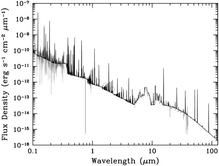
Figure 12.— The predicted SED from the P-I modeling (black line) and the observed spectrum of BoBn 1 from the $IUE$, Subaru/HDS, VLT/UVES, and $Spitzer$/IRS (gray lines). The circles are 2MASS data.

Figure 13.— The location of BoBn 1 and K 648 on the HR-diagram. The values of K 648 are from Rauch et al. (2002). The solid and broken lines represent the post-AGB He-burning evolution tracks of Vassiliadis & Wood (1994) for a metallicity of $\sim$ 0.5 $Z_{\odot}$.

To investigate the properties of the ionized gas, dust, and the PN central star in a self-consistent way, we have constructed a theoretical photo-ionization (P-I) model which aims to match the observed flux of emission lines and the spectral energy distribution (SED) between UV and mid-IR wavelength, using Cloudy c08.00 (Ferland 2004).

First, a rough value of the distance to BoBn 1 is necessary in fitting the observed fluxes. The distance to this object is estimated to be in the range between 16.5 and 29 kpc (see Table 1). Based on the assumption that BoBn 1 is a member of the Sagittarius dwarf galaxy, we fix the distance to be 24.8 kpc (Kunder & Chaboyer 2009). P-I model construction needs information about the incident SED from the central star and the elemental abundances, geometry, density distribution, and size of the nebula. Once one gets a proper prediction of line intensities from a proper modeling procedure, the central stellar physical properties employed in the P-I model can give us a hint of the nebular evolutionary history or that of its progenitor star. Especially, the central star temperature $T_{\star}$ and the SED of the PN central star are an important physical parameter in constructing the correct P-I model.

We estimated $T_{\star}$ of 125 930 $\pm$ 6100 K using the energy balance methods proposed by Gurzadyan (1997). Being guided by this $T_{\star}$, we used theoretical model atmosphere for a series of values of $T_{\rm eff}$ to supply the SED from the central star. We used Thomas Rauch’s non-LTE theoretical model atmospheres for halo stars ($[X,Y]$ = 0 and $[Z]$ = –1) with the surface gravity $\log$ g = 6.0, 6.125, 6.25, 6.375, 6.5, and 6.625. We varied $T_{\rm eff}$ and the luminosity $L_{\star}$ to match the observations.

For the elemental abundances X/H, we used the values from the case of $t^{2}$ = 0 as a starting point. For the C, N, O, and Ne abundances, we used the CELs abundances. We assumed no high-density cold clumps. Using the HDS slit-viewer image (Fig. 1), we measured the radius of the outer nebular shell $R_{\rm out}$ of $\sim$0.6^′′ (=0.072 pc) and fixed this value. We assumed the hydrogen density $N_{\rm H}$ to be a $R^{-2}$ smooth distribution, i.e., $N_{\rm H}$ = $N_{\rm H}$($R_{\rm in}$) $\times$ ($R_{\rm in}/R$)². In the models, within a small range we varied X/H, $N_{\rm H}$($R_{\rm in}$), and $R_{\rm in}$ to match the observed line fluxes from UV to mid-infrared wavelength, including 2MASS $JHK$ bands, and our mid-infrared bands, i.e., between 17 and 23 $\mu$m (IRS B) and between 27 and 33 $\mu$m (IRS C).

Since the IRS spectra show that the dust grains co-exist in the nebula of BoBn 1, we need information about the dust composition. Here we considered amorphous carbon and PAH grains. The optical constants were taken from Rouleau & Martin (1991) for amorphous carbon and from Desert et al. (1990), Schutte et al. (1993), Geballe (1989), and Bregman et al. (1989) for PAHs. The observed emission-line and base line continuum fluxes between 5.9 and 6.9 $\mu$m (PAH 6.4 $\mu$m) and between 7.4 and 8.4 $\mu$m (PAH 7.9 $\mu$m) were used to determine the PAH abundance. We assumed that the gas and dust co-exist in the same sized ionized nebula. We adopted a standard MRN $a^{-3.5}$ distribution (Mathis, Rumpl & Nordsieck 1977) with $a_{\rm min}$=0.001 $\mu$m and $a_{\rm max}$=0.25 $\mu$m for amorphous carbon. For PAHs we adopted an $a^{-4}$ size distribution with $a_{\rm min}$=0.00043 $\mu$m and $a_{\rm max}$=0.0011 $\mu$m. We adopted an $R^{-2}$ smooth dust density distribution. High-density clumped dust grains were not considered.

In Table 20, we compare the predicted with observed relative fluxes where $I$(H$\beta$) = 100. For most CELs and He lines and the wide band fluxes, as well, the agreement between the P-I model and the observation is within 30$\%$. The poor fit of [N i], [O i], and [S ii] would be due to the assumed density profile. The relation between $n_{\epsilon}$ and I.P. (Fig. 8 lower panel) shows that the electron density jumps from $\sim$2000 to $\sim$6000 cm^-3 around [S ii] emitting region. In our model, such a density jump was not considered. For important lines such as He i, ii, and C iii$]$, [N ii], [O ii], [O iii], [Ne iii], fairly good agreements in calculating ionic abundances are achieved. However, most of the C and O ORLs fit to the observations poorly. In most cases, the P-I models underestimate their line fluxes. As we discussed above, the O ORLs, and likely the Ne ORLs too, might be emitted from cold and metal-enhanced clumps.

In Table 21, we list the derived parameters of the PN central star, ionized nebula, and dust, and in Fig. 12 we present the predicted SED (black line). The predicted SED matches the UV to mid-infrared region well. Through the P-I modeling, we found the PN central star’s parameters: $T_{\rm eff}$ = 125 260 $\pm$ 200 K, $L_{\star}$ = 1180 $\pm$ 240 $L_{\odot}$, $\log$ g = 6.5, and a core mass of $\sim$0.62 $M_{\odot}$. The estimated 0.62 core mass is comparable to that of K 648 (0.62 $M_{\odot}$, Bianchi et al. 2001; 0.57 $M_{\odot}$ Rauch et al. 2002) and the high-excitation halo PN NGC 4361 (0.59 $M_{\odot}$: Traulsen et al. 2005). The ionized mass of BoBn 1 is 0.09 $M_{\odot}$, which is comparable to K 648 (0.07 $M_{\odot}$; Bianchi et al. 1995 ). In Fig. 13 we plot the locations of BoBn 1 and K 648 (Rauch et al. 2002) and the post-AGB He-burning evolutionary tracks for LMC metallicity ($Z$$\sim$0.5$Z_{\odot}$) by Vassiliadis & Wood (1994). These evolutionary tracks would suggest the possibility that the progenitors of BoBn 1 and K 648 were single 1-1.5 $M_{\odot}$ stars which would end their lives as white dwarfs with a core mass of $\sim$0.6 $M_{\odot}$. Alternatively, these halo PNe might have evolved from binaries composed of a 0.8 $M_{\odot}$ (= a typical halo star mass) secondary and a more massive primary, and gained mass ($\sim$0.1 $M_{\odot}$) from the primary through mass transfer or coalescence.

For K 648, Alves et al. (2000) support a binary evolution scenario. From F enhancement and similarity to carbon-enhanced metal poor stars (CEMP), Otsuka et al. (2008a) argued that BoBn 1 might have evolved from a binary composed of a 0.8 $M_{\odot}$ secondary and a $>$ 2 $M_{\odot}$ primary star. We should consider two possibilities: these halo PNe have evolved from single stars or from binaries.

The P-I model indicated elemental abundances except for C and S are in excellent agreement with those estimated by the empirical method using the ICFs. The discrepancy for C is due to the underprediction of C iv lines. The model predicted C⁺ = 2.0(–5) and C²⁺ = 3.4(–4), which are comparable to the observations. However, it predicted lower line fluxes of C iv $\lambda\lambda$1548/51 than the observations, and accordingly an underestimated C³⁺ as 6.95(–5). These might suggest that the origin of C iv lines is not the ionized nebula but the stellar wind zone. The discrepancy for S could be due to the low ionic the S⁺ abundance, which depends strongly on the assumed radial density profile.

For BoBn 1, we have for the first time estimated a dust mass of 5.78(–6) $M_{\odot}$ and the temperature of 80–180 K. The dust in BoBn 1 is carbon rich. The dust composition suggests that BoBn 1 had experienced the TDU during the latest thermal pulsing AGB phase (TP-AGB). Since the TDU efficiently takes place in $>$1 $M_{\odot}$ stars, the progenitor of BoBn 1 might be 1–3.5 $M_{\odot}$ from the aspect of elemental abundances and dust composition.

The dust-to-gas mass ratio $\psi$ of 5.84(–5) is much lower than the typical value in PNe ($<$$\sim$10^-3; Pottash 1984). For AGB stars, Lagadec et al. (2009) argued that $\psi$ scales linearly with the metallicity. They assume the ratio is

$$\psi=\psi_{\odot}\times 10^{[{\rm Fe/H}]}$$ (7)

where $\psi_{\odot}$ is 0.005. When we adopt $[$Fe/H$]$ = –2.22 for BoBn 1, we obtain $\psi$ = 3.01(–5).

Assuming that the inner and outer shells were expanding with $\sim$10 km s^-1 and most of the dust was formed during the ending period of the thermal pulse AGB phase, we estimated the dust mass-loss rate $\dot{M}$_dust of $\sim$3(–9) $M_{\odot}$ yr^-1. Lagadec et al. (2009) estimated $\dot{M}$_dust in metal-poor ([Fe/H]$\sim$–1) carbon stars IRAS16339-0317 and 18120+4530 in the Galactic halo and IRAS12560+1656 in the Sgr stream. They estimated 4–18(–9) $M_{\odot}$ yr^-1. For IRAS12560+1656, Groenewegen et al. (1997) estimated $\dot{M}$_dust of 1.9(–9) $M_{\odot}$ yr^-1. These $\dot{M}$_dust values are comparable to that of BoBn 1.

4.4. Comparison of observations and theoretical models

Through P-I modeling, we found two possibilities: BoBn 1 might have evolved from (a) a 1-1.5 $M_{\odot}$ single star or (b) a binary composing of $\sim$0.8 $M_{\odot}$ secondary and a more massive primary. In this section, we explore these possibilities by comparing the observed and predicted elemental abundances employing theoretical nucleosynthesis models for low- to intermediate mass stars.

In Table 22, we present observed elemental abundances and predicted values from the theoretical models of Karakas & Lugaro (2009) for 1.0, 1.5, and 2.0 $M_{\odot}$ stars with $Z$=10^-4 ([Fe/H]$\sim$–2.3). The abundances from the models are the values at the end of the AGB phase. For these models, Karakas & Lugaro (2009) chose an initial $\alpha$-enhanced abundance pattern, i.e., [$\alpha$/Fe]=+0.4. For s-process elements, they chose scaled solar abundances, i.e., [X/Fe]=0. These [$\alpha$/Fe] and [X/Fe] ratios are consistent with the values for RGB stars in Terzan 8, therefore the assumption of initial abundances seems very reasonable for BoBn 1. The accuracy of the predicted abundances by the models is within 0.3 dex. For the observed abundances, we adopted the $t^{2}$=0 CEL abundances except for C. The adopted C abundance was from ORLs.

On the possibility (a) that BoBn 1 has evolved from a single star and has survived in the Galactic halo, the abundances of BoBn 1 except for N can be properly explained by the 1.5 $M_{\odot}$ star model including a partial mixing zone of 0.004 $M_{\odot}$, which produces a ¹³C pocket during the interpulse period and releases free neutrons through ¹³C($\alpha$,n)¹⁶O. This model assumes that the stars end as white dwarfs with a core mass of $\sim$0.7 $M_{\odot}$, which is comparable to our estimated core mass.

The ¹³C($\alpha$,n)¹⁶O reaction proceeds in the upper surface layer of the He-burning shell. The F and s-process elements are synthesized by capturing these neutrons in the He-intershell. The observed F, probably Kr and Xe abundances are systematically larger ($\sim$+0.5 dex) than 1.5 $M_{\odot}$ star + partial mixing model. This suggests that hydrogen mixing mass is likely to be $>$ 0.004 $M_{\odot}$ or that BoBn1 had experienced helium-flash driven deep mixing (He-FDDM, Fujimoto et al. 2000; Suda et al. 2004) and obtained the extra neutrons. This process can occur in stars with [Fe/H] $<$–2.5 at the bottom of the He-burning shell because the entropy barrier between the H- and He-shell becomes low. The lower limit to [Fe/H] for BoBn1 is $-$2.46. This process would also produce ¹⁴N through the ¹³C($p$,$\gamma$)¹⁴N reaction, by mixing protons into the He-burning shell.

We note that BoBn 1 is similar to K 648, for the latter is also known as an extremely metal poor, C- and N-rich halo PN. On the assumption that K 648 has been evolved from a single star, the abundances of K 648 except for Ne can be explained by a 1.5 $M_{\odot}$ model. K 648 would not have experienced He-FDDM for abnormally increasing N.

However, can halo single stars with an initial mass of $\sim$1.5 $M_{\odot}$ and $Z$ = 10^-4 survive up to now? Such stars would end as white dwarfs in $\sim$2-3 Gyr. Their lifetime is much shorter than the age of Terzan 8; Forbes et al. (2004) estimated the age of Terzan 8 to be 13 $\pm$ 1.5 Gyr from an age-metallicity relation for the Sagittarius dwarf globular cluster. If the progenitor of BoBn 1 was a $\sim$0.8 $M_{\odot}$ single star, then it can have survived up to now, however it cannot evolve into a visible PN and cannot become extremely C-rich. To circumvent the evolutionary time scale problem, we should consider the other evolutionary scenario for BoBn 1.

Table 22Comparison of observations and the theoretical models for single and binary stars with $Z$=10^-4.

	Abundances ($\log$(X/H) + 12)
Model	C	N	O	F	Ne	Fe	Kr	Xe
1.00 $M_{\odot}$	8.13	6.52	6.98	3.79	6.45	5.18	2.00	0.97
1.50 $M_{\odot}$	9.21	6.81	7.76	5.28	8.11	5.21	2.43	1.46
+ partial mixing	9.17	6.78	7.85	5.30	8.31	5.21	2.47	1.50
2.00 $M_{\odot}$	9.55	6.87	7.92	5.93	8.66	5.24	2.37	1.53
0.75 $M_{\odot}$ + 1.50 $M_{\odot}$	9.51	7.09	7.67	5.04	7.47	5.22	2.11	1.30
0.75 $M_{\odot}$ + 1.80 $M_{\odot}$	9.31	6.72	7.50	4.74	7.17	5.20	1.88	1.07
0.75 $M_{\odot}$ + 2.10 $M_{\odot}$	9.23	6.58	7.41	4.69	7.11	5.20	1.73	0.91
BoBn 1 ($t^{2}$=0)	9.16	8.03	7.74	5.85	7.96	5.08	$<$2.88	$<$1.97
K 648 ($t^{2}$=0)	9.25	6.36	7.78	$\dots$	6.87	$\dots$	$\dots$	$\dots$

4.5. The Origin of BoBn 1

As mentioned earlier, BoBn 1 is likely to be a binary origin because the [C,N,F/Fe] abundances of BoBn 1 are comparable to those of the carbon-enhanced metal poor star (CEMP) HE 1305+0132 (Schuler et al. 2007) and other CEMP stars.

Most CEMP stars show large enhancements of C and N abundances. Some evolutionary models for CEMP stars have demonstrated that the C and N overabundances would be reproduced by binary interactions. Schuler et al. (2007) concluded that HE 1305+0132 might have experienced mass transfer and that s-process elements should be enhanced. Lugaro et al. (2008) concluded that HE 1305+0132 consisted of $\sim$2 M_⊙ (primary) and $\sim$0.8 M_⊙ (secondary) stars with Z = 10^-4 and that the enhanced C and F could be explained by binary mass transfer from the primary star via Roche lobe overflow and/or wind accretion. In Fig. 14, we present the diagram of [Xe,Ba/Ar]-[C/Ar]. The [Xe/Ar] for BoBn 1 is an upper limit. The data for Galactic PNe except BoBn 1 are taken from Sharpee et al. (2007). The data for s-process elements enhanced CEMP (CEMP-s) with [Fe/H] $>$ –2.5 and C-rich AGB are from the SAGA data base (Suda et al. 2008). For PNe, we use Xe as a heavy s-process element and adopt Ar as a metallicity reference. For CEMP-s and C-rich AGB stars, we use Ba and Fe as a metallicity reference. The diagram indicates that C and s-process elements are certainly synthesized in the same layer and brought up to the stellar surface by the TDU. We note that the enhancement of heavy s-process elements in BoBn1 is comparable to CEMP-s stars, in particular CS22948-027 (Aoki et al. 2007;[Fe/H] = –2.21, [Ba/Fe] = +2.31, [C/Fe] = +2.12, [N/Fe] = +2.48). The chemical similarities between BoBn 1 and CEMP-s stars suggest that this PN shares a similar origin and evolutionary history.

BoBn 1 is similar to K 648 in elemental abundances and nebular shape (see Fig. 1 and Table 19). K 648 has been for a long time suspected to have experienced binary evolution. Rauch et al. (2002) and Bianchi et al. (2001) analyzed the spectrum of the central star and estimated a core mass $\sim$0.6 $M_{\odot}$. The mass $\sim$0.6 $M_{\odot}$ corresponds to the initial mass of 1-1.5 $M_{\odot}$ from the HR-diagram as shown in Fig. 13. The initial mass of 1-1.5 $M_{\odot}$ suggests that K 648 might have evolved from a binary and accreted a part of the ejected mass by a massive primary or coalescence during the evolution. Alves et al. (2000) argued that K 648 has experienced mass augmentation in a close-binary merger and evolved as a higher mass star to become a PN. Such a high mass star would be a blue straggler. Ferraro et al. (2009) observed stars in the globular cluster M 30 using the $HST$/WFPC2 and concluded that blue stragglers are results of coalescence or binary mass-transfer.

In view of the internal kinematics and chemical abundances, the progenitor of K 648 seems to be a binary. K 648 has a bipolar outflow (Tajitsu & Otsuka 2006) and bipolar nebula (Alves et al. 2000). The statistical study of PN morphology shows that bipolar PNe have evolved from massive stars with initial mass $\gtrsim$ 2.4 $M_{\odot}$ or binaries. Otsuka et al. (2008b) showed that the [C/Fe] and [N/Fe] abundances of K 648 are compatible with CEMP stars. So far, there have been no reports on the detection for any binary signatures in both objects. The contradiction to the evolutionary time scale of this object can be avoided if BoBn 1 has indeed evolved from a binary. Similar to K 648, BoBn 1 could have evolved from a binary and undergone coalescence to become a PN.

We explore the possibility of binary evolution of BoBn 1 using binary nucleosynthesis models by Izzard et al. (2004, 2009). We assume a binary system composed initially of a 0.75 $M_{\odot}$ secondary and a 1.5/1.8/2.1 $M_{\odot}$ primary with $Z$=10^-4, separation = 219/340/468 $R_{\odot}$, respectively. We set eccentricity $e$ = 0, common envelope efficiency $\alpha$ = 0.5 and structure parameter $\lambda_{\rm CE}$ = 0.5. He-FDDM is not considered. We set a ¹³C pocket mass of 7.4$\times$10^-4 $M_{\odot}$. The ¹³C pocket contains 4.1$\times$10^-6 $M_{\odot}$ ¹³C and 1.3$\times$10^-7 $M_{\odot}$ ¹⁴N. We set the ¹³C pocket efficiency = 2 and adopt wind mass-loss rates from Reimers formula on the RGB and by Vassiliadis & Wood (1993) on the TP AGB.

When we choose these initial primary and secondary masses and $\alpha$, the binary system will experience Roche lobe overflow; and it will merge into a 1.2-1.4 $M_{\odot}$ single star at the TP-AGB phase and end its life as a white dwarf with a core mass of 0.62-0.68 $M_{\odot}$, 10.4-12.5 Gyr after the progenitor was born. We present the results in Table 22. The binary models might seem to explain the elemental abundances of BoBn 1 and K 648. Concerning K 648, the 0.75 $M_{\odot}$ + 1.5 $M_{\odot}$/1.8 $M_{\odot}$ models fairly well match the prediction to the observed abundances. Among the models, the 0.75 $M_{\odot}$ + 1.5 $M_{\odot}$ model seems to be the best fit to BoBn 1 for the moment because this model can explain not only the abundance patterns but also the observed core mass (the predicted core mass $\sim$0.64 $M_{\odot}$). If the progenitor has experienced extra mixing in the RGB phase and increased N, the N overabundance can be accommodated by this model. The issues with the evolutionary time scale and C and N enhancements might be resolved simultaneously if BoBn 1 has evolved from such a binary. At the present, we conclude consider that binary evolution scenario is more plausible for BoBn 1.

To discuss further the evolution of BoBn 1 and K 648, we need to increase detection cases of s-process elements and to investigate the isotope ratios of ¹²C/¹³C, ¹⁴N/¹⁵N, ¹⁶O/¹⁷O, and ¹⁶O/¹⁸O, which would be useful to investigate nucleosynthesis in the progenitors. It would be also necessary to completely trace mass-loss history to improve mass-loss rate. So far, mass-loss history of evolved stars has been revealing by investigating spatial distribution of dust grains and molecular gas using far-infrared to millimeter wavelength data. The Atacama Large Millimeter Array (ALMA) and the thirty meter telescope (TMT) could open new windows to study the evolution of metal-poor stars such as halo PNe.

Figure 14.— [Xe or Ba/Ar]-[C/Ar] diagram. The [Xe/Ar] value of BoBn 1 is upper limit. For PNe, we adopt Ar as a metallicity reference. For CEMP-s and C-rich AGB stars, we use Fe as a metallicity reference.

5. Conclusion

We have performed a comprehensive chemical abundance analysis of BoBn 1 using $IUE$ archive data, Subaru/HDS spectra, VLT/UVES archive data, and $Spitzer$/IRS spectra. We calculated the ionic and elemental abundances of 13 elements using ORLs and CELs. The estimations of C, N, O, and Ne abundances from the ORLs and Kr, Xe, and Ba from the CELs are done for the first time. The C, N, O, and Ne ORL abundances are systematically larger than those from CELs. We investigated the cause of the abundance discrepancies. The discrepancies except for O could be explained by a temperature fluctuation model, and that of O might be due to hydrogen deficient cold components.

In the optical high-dispersion spectra, we detected emission-lines of fluorine and s-process elements such as rubidium, krypton, xenon, and barium. The values of [F/H], [Kr/H], and [Xe/H] suggest that BoBn 1 is the most F-rich among F detected PNe and is a heavy s-process element rich PN. The enhancement of C, N, and heavy s-process is comparable to CEMP-s stars with [Fe/H] $>$–2.5. This suggests that BoBn 1 shares a similar origin and evolutionary history with CEMP-s stars.

We built photo-ionization model using non-LTE theoretical stellar atmosphere models to check consistency between elemental abundances derived by empirical methods and from the model and to investigate the properties of the central star, ionized nebula, and dust in a self-consistent way to fit the IR wavelength region. In the modeling, we considered the presence of dust. We compared the observed elemental abundances with theoretical nucleosynthesis model predictions for single stars and binaries with $Z$ = 10^-4. The observed elemental abundances except for N could be explained either by a 1.5 $M_{\odot}$ single star model or a binary model composed of 0.75 $M_{\odot}$ + 1.5 $M_{\odot}$ stars. Through the modeling, we estimated the luminosity and effective temperature and surface gravity of the central star and the total mass of ionized gas and dust and even for the SED of BoBn 1. Using theoretical evolutionary tracks for post-AGB stars, we found that the progenitor of the central star was perhaps a 1-1.5 $M_{\odot}$ star and evolved into a system of a white dwarf with a core mass of $\sim$0.62 $M_{\odot}$ and an $\sim$0.09 $M_{\odot}$ ionized nebula. We estimated a total mass of 5.8$\times$10^-6 $M_{\odot}$ in the nebula, which composes of amorphous carbon and PAHs. The presence of carbon dust indicates that BoBn 1 has experienced the third dredge-up during the thermal pulse AGB phase.

The progenitor might have been initially quite N-rich. The He-flash driven deep mixing might be responsible for the overabundance of N. From careful consideration of observational results and a comparison between BoBn 1 and K 648 in M 15, we propose that the progenitor was a 0.75 $M_{\odot}$ + 1.5 $M_{\odot}$ binary with, e.g. an initial separation of 219 $R_{\odot}$ and had experienced coalescence during its evolution to become a C- and N-rich PN. The similar evolutionary scenario would be also applicable to K 648.

Appendix A Observed line list (on-line table).

Table 23Observed and reddening corrected line ratios [$I(\rm H\beta)$=100] and identifications of BoBn 1. The few lines from the Table A1.

$\lambda_{\rm obs}$	Ion	$\lambda_{\rm lab}$	Comp.	$f(\lambda)$	$I(\lambda)$	$\delta$$I(\lambda)$	Source	Note
(Å)		(Å)
3301.48	O iii	3299.39	1	0.423	0.632	0.031	UVES1
3314.43	O iii	3312.33	1	0.418	1.644	0.038	UVES1
3336.76	Ne ii	3334.87	1	0.411	0.104	0.019	UVES1
$\cdots$
4717.13	[Ne iv]	4714.25	1	0.041	0.055	0.003	HDS
4718.61	[Ne iv]	4715.80	1	0.041	0.019	0.002	HDS
4727.07	[Ne iv]	4724.15	1	0.039	0.051	0.002	HDS
4728.51	[Ne iv]	4725.62	1	0.038	0.045	0.003	HDS
4743.20	[Ar iv]	4740.17	1	0.034	0.090	0.004	HDS
4757.92	[Fe iii]	4754.69	1	0.030	0.021	0.005	HDS
4788.04	C iv?	4785.90	1	0.021	0.044	0.005	HDS
4790.11	N iv	4786.92	1	0.020	0.013	0.005	UVES1
4792.87	[F ii]	4789.45	1	0.020	0.056	0.005	HDS
4801.07	[Fe ii]	4798.27	1	0.017	0.008	0.005	HDS
4805.62	Ne ii	4802.58	1	0.016	0.034	0.006	HDS
4855.14	He ii	4852.00	1.00	0.003	0.007	0.004	HDS	Raman line?
4856.93	[Fe iii]	4853.70	1	0.002	0.004	0.003	HDS
4862.36	He ii	4859.32	1	0.001	0.869	0.130	HDS
4864.46	H4	4861.33	1	0.000	100.000	0.202	HDS
4872.75	[F ii]	4868.99	1	–0.002	0.013	0.003	HDS
4879.17	[Co vi]	4876.26	1	–0.004	0.009	0.004	HDS
4884.34	[Fe iii]	4881.00	1	–0.005	0.021	0.005	HDS
4924.71	He i	4921.93	1	–0.016	0.277	0.011	UVES1
4925.21	He i	4921.93	2	–0.016	1.043	0.013	UVES1
			Tot.		1.320	0.017	UVES1
4934.42	[O iii]	4931.23	1	–0.019	0.044	0.004	HDS
4937.32	Ba ii	4934.08	1	–0.019	0.006	0.002	UVES1
4961.87	[O iii]	4958.91	1	–0.026	29.603	2.389	HDS
4962.03	[O iii]	4958.91	2	–0.026	32.311	1.991	HDS
4962.28	[O iii]	4958.91	3	–0.026	60.490	5.079	HDS
			Tot.		122.404	5.956	HDS
4967.84	C ii	4964.73	1	–0.027	0.027	0.004	HDS
5004.63	N ii	5001.47	1	–0.036	0.018	0.003	HDS
5009.85	[O iii]	5006.84	1	–0.038	55.674	13.550	HDS
5009.97	[O iii]	5006.84	2	–0.038	137.072	3.874	HDS
5010.25	[O iii]	5006.84	3	–0.038	158.090	16.602	HDS
			Tot.		350.836	21.776	HDS
5018.53	He i	5015.68	1	–0.040	0.291	0.012	HDS
5019.01	He i	5015.68	2	–0.040	1.481	0.014	HDS
			Tot.		1.772	0.019	HDS
5033.51	[Fe iv]	5030.33	1	–0.043	0.089	0.008	HDS
5035.14	C ii	5032.07	1	–0.044	0.053	0.005	HDS
5038.93	[Fe ii]	5035.48	1	–0.045	0.011	0.004	HDS
5039.16	C ii	5035.94	1	–0.045	0.018	0.003	UVES1
5050.58	He i	5047.74	1	–0.048	0.044	0.009	HDS
5051.11	He i	5047.74	2	–0.048	0.211	0.011	HDS
			Tot.		0.254	0.014
5059.25	Si ii	5055.98	1	–0.050	0.007	0.004	UVES2
5069.55	N ii	5066.46	1	–0.052	0.042	0.009	UVES2
5117.37	O v	5114.06	1	–0.063	0.013	0.030	HDS
5122.44	[Fe iii]	5119.97	1	–0.065	0.014	0.004	HDS
5125.06	C ii	5121.83	1	–0.065	0.029	0.002	HDS
5130.66	Fe iii	5127.39	1	–0.066	0.007	0.002	HDS
$\cdots$
9074.84	[S iii]	9068.60	1	–0.594	0.378	0.010	UVES2
9101.95	N ii	9096.16	1	–0.596	0.011	0.004	UVES2
9114.25	He ii	9108.54	1	–0.597	0.032	0.003	UVES2
9205.28	Fe i	9199.45	1	–0.603	0.012	0.002	UVES2
9216.31	He i	9210.34	1	–0.604	0.093	0.006	UVES2
9219.44	He i	9213.24	1	–0.604	0.025	0.004	UVES2
9223.29	Mg ii?	9218.25	1	–0.604	0.008	0.003	UVES2
9230.87	He ii	9225.23	1	–0.605	0.032	0.006	UVES2
9234.92	H i	9229.01	1	–0.605	2.545	0.043	UVES2
9350.69	He ii	9344.94	1	–0.613	0.572	0.011	UVES2

References

- (1) Acker, A., Marcout, J., Ochsenbein, F., Stenholm, B., & Tylenda, R. 1992, “Strasbourg - ESO catalogue of galactic planetary nebulae. Part 1; Part 2”
- (2) Aldrovandi, S. M. V. 1980, Ap&SS, 71, 393
- (3) Aller, L. H. 1984 “Physics of Thermal Gaseous Nebulae”, Astrophysics & Space Science Library vol. 112
- (4) Alves, D. R., Bond, H. E., & Livio, M. 2000, AJ, 120, 2044
- (5) Aoki, W., Beers, T. C., Christlieb, N., Norris, J. E., Ryan, S. G., & Tsangarides, S. 2007, ApJ, 655, 492
- (6) Badnell, N. R., & Pindzola, M. S., 2000, J. Phys. B., 33, 1013
- (7) Baluja, K. L., & Zeippen, C. J. 1988, J. Phys. B, 21, 1455
- (8) Barker, T. 1980, ApJ, 237, 482
- (9) Barker, T. 1983, ApJ, 270, 641
- (10) Barlow, M. J., Hales, A. S., Storey, P. J., Liu, X.-W., Tsamis, Y. G., & Aderin, M. E. 2006, IAU Symposium, 234, 367
- (11) Bernard-Salas, J., Peeters, E., Sloan, G. C., Gutenkunst, S., Matsuura, M., Tielens, A. G. G. M., Zijlstra, A. A., & Houck, J. R. 2009, ApJ, 699, 1541
- (12) Becker, S. R., Butler, K., & Zeippen, C. J. 1989, A&A, 221, 375
- (13) Benjamin, R. A., Skillman, E. D., & Smits, D. P. 1999, ApJ, 514, 307
- (14) Berrington, K. A., Burke, P. G., Dufton, P. L., & Kingston, A. E. 1985, Atomic Data and Nuclear Data Tables, 33, 195
- (15) Bhatia, A. K., & Kastner, S. O. 1995, ApJS, 96, 325
- (16) Bhatia, A. K., & Doschek, G. A. 1993, Atomic Data and Nuclear Data Tables, 55, 315
- (17) Bhatia, A. K., & Kastner, S. O. 1988, ApJ, 332, 1063
- (18) Bianchi, L., Bohlin, R., Catanzaro, G., Ford, H., & Manchado, A. 2001, AJ, 122, 1538
- (19) Bianchi, L., Ford, H., Bohlin, R., Paresce, F., & de Marchi, G. 1995, A&A, 301, 537
- (20) Biémont, E., Hansen, J. E., Quinet, P., & Zeippen, C. J. 1995, A&A, 333, 346
- (21) Biémont, E., & Hansen, J. E. 1986, Phys. Scr. 33, 117
- (22) Blum, D. & Pradhan, A. K. 1992, ApJS, 80, 425
- (23) Boeshaar, G. O., & Bond, H. E. 1977, ApJ, 213, 421
- (24) Brage, T., Fischer, C. F., & Judge, P. G. 1995, ApJ, 445, 457
- (25) Bregman, J. D., Allamandola, L. J., Witteborn, F. C., Tielens,A. G. G. M., & Geballe, T. R., 1989, ApJ, 344, 791
- (26) Butler, K., & Zeippen, C. J. 1994, A&AS, 108, 1
- (27) Cahn, J. H., Kaler, J. B., & Stanghellini, L. 1992, A&AS, 94, 399
- (28) Cardelli, J. A., Clayton, G. C., & Mathis, J. S. 1989, ApJ, 345, 245
- (29) Copetti, M. V. F., & Writzl, B. C. 2002, A&A, 382, 282
- (30) Cuisinier, F., Acker, A., & Köppen, J. 1996, A&A, 307, 215
- (31) Davey, A. R., Storey, P. J., & Kisielius, R. 2000, A&AS, 142, 85
- (32) Dekker, H., D’Odorico, S., Kaufer, A., Delabre, B., & Kotzlowski, H. 2000, SPIE, 4008, 534
- (33) Desert, F.-X., Boulanger, F., & Puget, J.L. 1990, A&A, 237, 215
- (34) Dopita, M. A., Mason, D. J., & Robb, W. D. 1976, ApJ, 207, 102
- (35) Dufton, P. L., Hibbert, A., Kingston, A. E., & Doschek, G. A. 1982, ApJ, 257, 338
- (36) Ellis, D. G., & Martinson, I. 1984, Phys. Scr., 30, 255
- (37) Escalante, V., & Victor, G. A. 1990, ApJS, 73, 513
- (38) Ferland, G. J. 2004, Bulletin of the American Astronomical Society, 36, 1574
- (39) Ferraro, F. R., et al. 2009, Nature, 462, 1028
- (40) Forbes, D. A., Strader, J., & Brodie, J. P. 2004, AJ,127, 3394
- (41) Froese-Fischer, C. 1994, Phys. Scr, 49, 323
- (42) Froese-Fischer, C., & Rubin, R. H. 1998, J. Phys. B., 31, 1657
- (43) Froese-Fischer C., & Saha, H. P. 1985, Phys. Scr., 32, 181
- (44) Froese-Fischer, C., 1983, J. Phys. B., 16, 157
- (45) Froese-Fischer, C., Tachiev, G., & Irimia, A. 2006, ADNDT, 92, 607
- (46) Fujimoto, M. Y., Ikeda, Y. & Iben, I. Jr. 2000, ApJL, 529, 25
- (47) Galavis, M. E., Mendoza, C., & Zeippen, C. J. 1995, A&AS, 111, 347
- (48) Garnett, D. R., & Lacy, J. H. 1993, ApJ, 419, L93
- (49) Garstang, R. H. 1958, MNRAS, 118, 572
- (50) Garstang, R. H. 1957, MNRAS, 117, 393
- (51) Garstang, R. H. 1951, MNRAS, 111, 115
- (52) Geballe, T. R., 1989, ApJ, 344, 791
- (53) Georgiev, L. N., Peimbert, M., Hillier, D. J., Richer, M. G., Arrieta, A., & Peimbert, A. 2008, ApJ, 681, 333
- (54) Grandi, S. A. 1976, ApJ, 206, 658
- (55) Groenewegen, M. A. T., Oudmaijer, R. D., & Ludwig, H.-G. 1997, MNRAS, 292, 686
- (56) Gurzadyan, G. A. 1997, “The Physics and Dynamics of Planetary Nebulae”, Springer-Verlag Berlin Heidelberg New York.
- (57) Hawley, S. A., & Miller, J. S. 1978, ApJ, 220, 609
- (58) Henry, R. B. C., Kwitter, K. B., & Balick, B. 2004, AJ, 127, 2284
- (59) Houck, J. R., et al. 2004, SPIE, 5487, 62
- (60) Howard, J. W., Henry, R. B. C., & McCartney, S. 1997, MNRAS, 284, 465
- (61) Izzard, R. G., Tout, C. A., Karakas, A. I., & Pols, O. R. 2004, MNRAS, 350, 407
- (62) Izzard, R. G., Glebbeek, E., Stancliffe, R. J., & Pols, O. R. 2009, A&A, 508, 1359
- (63) Jacoby, G. H., & Ford, H. C. 1983, ApJ, 1983, 266, 298
- (64) Johnson, C. T., Burke, P. G., & Kingston, A. E. 1987, J. Phys. B, 20, 2553
- (65) Johnson, C. T., Kingston, A. E., & Dufton, P. L. 1986, MNRAS, 220, 155
- (66) Karakas, A. I., & Lattanzio, J. C. 2003, PASA, 20, 393
- (67) Karakas, A. I. 2010, MNRAS, 403, 1413
- (68) Karakas, A. I., & Lugaro, M. 2009, arXiv:0909:5001
- (69) Kaufman, V., & Sugar, J. 1986, JPCRD, 15, 321
- (70) Keenan, F. P., Hibbert, A., Ojha, P. C., & Caylon, E. S. 1993, Phys. Scr., 48, 129
- (71) Kingdon, J., & Ferland, G. J. 1995, ApJ, 442, 714
- (72) Kingsburgh, R. L., & Barlow, M. J. 1992, MNRAS, 257, 317
- (73) Kisielius, R., & Storey, P. J. 2002, A&A, 387, 1135
- (74) Kisielius, R., Storey, P. J., Davey, A. R., & Neale, L. T., 1998, A&AS, 133, 257
- (75) Klose, J. Z., Fuhr, J. R., & Weise, W. L. 2002, J. Phys. Chem. Rev. Data, 31, 217 Ba2 A
- (76) Kniazev, A. Y., et al. 2008, MNRAS, 388, 1667
- (77) Komiya, Y., Suda, T., Minaguchi, H., Shigeyama, T., Aoki, W., & Fujimoto, M. Y. 2007, ApJ, 658, 367
- (78) Kunder, A., & Chaboyer, B. 2009, AJ, 137, 4478
- (79) Kwitter, K. B., & Henry, R. B. C., Milingo, J. B. 2003, PASP, 115, 80
- (80) Kwitter, K. B., & Henry, R. B. C. 1996, ApJ, 473, 304
- (81) Lagadec, E., Zijlstra, A., Mauron, N., Fuller, G., Josselin, E., Sloan, G. C., & Riggs, A. J. E. 2009, arXiv:0911.4376
- (82) Lau, H. H. B., Stancliffe, R. J., & Tout, C. A. 2007, MNRAS, 378, 563
- (83) Lennon, D. J., & Burke, V. M. 1994, A&AS, 103, 273
- (84) Liu, Y., Liu, X.-W., Barlow, M. J., & Luo, S.-G. 2004, MNRAS, 353, 1251
- (85) Liu, X.-W., Luo, S.-G., Barlow, M. J., Danziger, I. J., & Storey, P. J. 2001, MNRAS, 327, 141
- (86) Liu, X.-W., Storey, P. J., Barlow, M. J., & Clegg, R. E. S. 1995, MNRAS, 272, 369
- (87) Liu, X.-W., Storey, P. J., Barlow, M. J., Danziger, I. J., Cohen, M., & Bryce, M. 2000, MNRAS, 312, 585
- (88) Lodders, K. 2003, ApJ, 591, 1220
- (89) Lugaro, M., et al. 2008, A&A, 484, L27
- (90) Mal’Kov, Y. F. 1997, Astronomy Reports, 41, 760
- (91) Martin, I., Karwowski, J., Diercksen, G. H. F., & Barrientos, C., 1993, A&AS, 100, 595
- (92) Mathis, J. S., Rumpl, W., & Nordsieck, K. H. 1977, ApJ, 217, 425
- (93) McLaughlin B. M., & Bell K. L., 2000, J. Phys. B., 33, 597
- (94) McLaughlin, B. M., & Bell, K. L. 1993, ApJ, 408, 753
- (95) Mendoza, C. 1983, in Flower, D. R. ed., ”Planetary Nebulae”, Kluwer Dordrecht, 143
- (96) Mendoza, C. & Zeippen, C. J. 1982a, MNRAS, 198, 127
- (97) Mendoza, C. & Zeippen, C. J. 1982b, MNRAS, 199, 1025
- (98) Morisset, C., & Georgiev, L. 2009, A&A, 507, 1517
- (99) Mottini, M., Wallerstein, G., & McWilliam, A. 2008, AJ, 136, 614
- (100) Nahar, S. N., & Pradhan, A. K. 1996, A&AS, 119, 509
- (101) Naqvi, A. M. 1951 Thesis Harvard 1951
- (102) Noguchi, K., et al. 2002, PASJ, 54, 855
- (103) Nussbaumer, H., & Storey, P. J. 1984, A&AS, 56, 293
- (104) Nussbaumer, H., & Storey, P. J. 1981, A&A, 96, 91
- (105) Otsuka, M. 2007, Doctoral Thesis Tohoku Univ. (Japan)
- (106) Otsuka, M., Hyung, S., Lee, S.-J., Izumiura, H., & Tajitsu, A. 2009, ApJ, 705, 509
- (107) Otsuka, M., Izumiura, H., Tajitsu, A., & Hyung, S. 2008a, ApJ, 682, L105
- (108) Otsuka, M., Izumiura, H., Tajitsu, A., & Hyung, S. 2008b, Origin of Matter and Evolution of Galaxies, 1016, 427
- (109) Otsuka, M., Tajitsu, A., & Tamura, S. 2006, IAU Symposium, 234, 235
- (110) Otsuka, M., Tamura, S., Yadoumaru, Y., & Tajitsu, A. 2003, PASP, 115, 67
- (111) Pease, F. G. 1928, PASP, 40, 342
- (112) Peimbert, M. 1967, ApJ, 150, 825
- (113) Peña, M., Torres-Peimbert, S., & Ruiz, M. T. 1991, PASP, 103, 865
- (114) Péquignot, D., et al. 2002, RMxAA Conference Series, 12, 142
- (115) Péquignot, D., Petitjean, P., & Boisson, C. 1991, A&A, 251, 680
- (116) Péquignot, D., & Aldrovandi, S. M. V. 1976, A&A, 50, 141
- (117) Persson, W., & Petterson, S.-G. 1984, Phys. Scr., 29, 308
- (118) Peeters, E., Hony, S., Van Kerckhoven, C., Tielens, A. G. G. M., Allamandola, L. J., Hudgins, D. M., & Bauschlicher, C. W. 2002, A&A, 390, 1089
- (119) Pradhan, A. K. 1976, MNRAS, 177, 31
- (120) Pottasch, S. R. 1984, “Planetary Nebulae”, Astrophysics and Space Science Library, 107,
- (121) Ramsbottom, C. A., Bell, K. L., & Keenan, F. P. 2001, Atomic Data & Nuclear Data Tables, 77, 57
- (122) Ramsbottom, C. A., Bell, K. L., & Keenan, F. P. 1998, MNRAS, 293, 233
- (123) Ramsbottom, C. A., Bell, K. L., & Stafford R. P., 1996, ADNDT 63, 57
- (124) Ramsbottom, C. A., Berrington, K. A., Hibbert, A., & Bell, K. L., Pyhs. Scripta, 1994, 50, 246
- (125) Rauch, T., Heber, U., & Werner, K. 2002, A&A, 381, 1007
- (126) Robertson-Tessi, M., & Garnett, D. R. 2005, ApJS, 157, 371
- (127) Robinson, G. J., Reay, N. K., & Atherton, P. D. 1982, MNRAS, 199, 649
- (128) Rouleau, F., & Martin, P. G. 1991, ApJ, 377, 526
- (129) Rubin, R. H. 1989, ApJS, 69, 897
- (130) Saraph, H. E. & Tully, J. A., 1994, A&AS, 107, 29
- (131) Schlegel, D. J., Finkbeiner, D. P., & Davis, M. 1998, ApJ, 500, 525
- (132) Schuler, S. C., Cunha, K., Smith, V. V., Sivarani, T., Beers, T. C., & Lee, Y. S. 2007, ApJ, 667, L81
- (133) Schutte, W. A., Tielens, A. G. G. M., & Allamandolla, L. J., 1993, ApJ, 415, 397
- (134) Schöning, T. 1997, A&A, 122, 277
- (135) Schöning, T., & Butler, K. 1998, A&A, 128, 581
- (136) Seaton, M. J. 1958, Reviews of Modern Physics, 30, 979
- (137) Seaton, M. J. 1979, MNRAS, 187, 73P
- (138) Sharpee, B., Zhang, Y., Williams, R., Pellegrini, E., Cavagnolo, K., Baldwin, J. A., Phillips, M., & Liu, X.-W. 2007, ApJ, 659, 1265
- (139) Sneden, C., Pilachowski, C. A., & Kraft, R. P. 2000, AJ, 120, 1351
- (140) Stancliffe, R. J. 2010, MNRAS, 403, 505
- (141) Stanghellini, L., & Kaler, J. B. 1989, ApJ, 343, 811
- (142) Storey, P. J. A&A, 1994, 282, 999
- (143) Storey, P. J., & Hummer, D. G. 1995, MNRAS, 272, 41
- (144) Storey, P. J., & Zeippen, C. J. 2000, MNRAS, 312, 813
- (145) Suda, T., et al. 2008, PASJ, 60, 1159
- (146) Suda, T., Aikawa, M., Machida, M. N., Fujimoto, M. Y., & Iben, I.Jr. 2004, ApJ, 611, 476
- (147) Tajitsu, A., & Otsuka, M. 2006, IAU Symposium, 234, 523
- (148) Tayal, S. S., & Gupta, R. P., 1999, ApJ, 526, 544
- (149) Torres-Peimbert, S., Peimbert, M., & Daltabuit, E. 1980, ApJ, 238, 133
- (150) Torres-Peimbert, S., Rayo, J. F., & Peimbert, M. 1981, RMxAA, 6, 6, 315
- (151) Traulsen, I., Hoffmann, A. I. D., Rauch, T., Werner, K., Dreizler, S., & Kruk, J. W. 2005, 14th European Workshop on White Dwarfs, 334, 325
- (152) Tsamis, Y. G., Barlow, M. J., Liu, X.-W., Danziger, I. J., & Storey, P. J. 2003, MNRAS, 338, 687
- (153) Tsamis, Y. G., Barlow, M. J., Liu, X.-W., Storey, P. J., & Danziger, I. J. 2004, MNRAS, 353, 953
- (154) van Diedenhoven, B., Peeters, E., Van Kerckhoven, C., Hony, S., Hudgins, D. M., Allamandola, L. J., & Tielens, A. G. G. M. 2004, ApJ, 611, 928
- (155) Vassiliadis, E., & Wood, P. R. 1994, ApJS, 92, 125
- (156) Vassiliadis, E., & Wood, P. R. 1993, ApJ, 413, 641
- (157) Verner, D. A., Verner, E. M., & Ferland, G. J. 1996, ADNDT, 64, 1
- (158) Viegas, S. M., & Clegg, R. E. S. 1994, MNRAS, 271, 993
- (159) Wang, W., & Liu, X.-W. 2007, MNRAS, 381, 669
- (160) Wang, W., Liu, X.-W., Zhang, Y., & Barlow, M. J. 2004, A&A, 427, 873
- (161) Wesson, R., Liu, X.-W., & Barlow, M. J. 2005, MNRAS,362, 424
- (162) Wesson, R., Liu, X.-W., & Barlow, M. J. 2003, MNRAS, 340, 253
- (163) Wiese, W. L., Fuhr, J. R., & Deters, T. M. 1996, J.Phys.Chem.Ref.Data,Monograph No.7, “Atomic Transition Probabilities of Carbon, Nitrogen and Oxygen”, American Chemical Society, Washington,DC, and American Institute of Physics, New York
- (164) Wright, S. A., Corradi, R. L. M., & Perinotto, M. 2005,A&A, 436, 967
- (165) Zeippen, C. J., Butler, K., & Le Bourlot, J. 1987, A&A, 188, 251
- (166) Zhang, H. 1996, A&AS, 119, 523
- (167) Zhang, H. L., & Pradhan, A. K. 1997, A&AS, 126, 373
- (168) Zhang, Y., & Liu, X.-W. 2005, ApJ, 631, L61
- (169) Zhang, Y., Liu, X.-W., Luo, S.-G., Péquignot, D., & Barlow, M. J. 2005a, A&A, 442, 249
- (170) Zhang, Y., Liu, X.-W., Liu, Y., & Rubin, R. H. 2005b, MNRAS, 358, 457
- (171) Zhang, Y., Liu, X.-W., Wesson, R., Storey, P. J., Liu, Y., & Danziger, I. J. 2004, MNRAS, 351, 935
- (172) Zijlstra, A. A., Gesicki, K., Walsh, J. R., Péquignot, D., van Hoof, P. A. M., & Minniti, D. 2006, MNRAS, 369, 875