Accurate photoionisation cross section for He at non-resonant photon energies

Abstract

The total single-photon ionisation cross section was calculated for helium atoms in their ground state. Using a full configuration-interaction approach the photoionisation cross section was extracted from the complex-scaled resolvent. In the energy range from ionisation threshold to 59 eV our results agree with an earlier $B$-spline based calculation in which the continuum is box discretised within a relative error of $0.01\%$ in the non-resonant part of the spectrum. Above the $\mathrm{He}^{++}$ threshold our results agree on the other hand very well to a recent Floquet calculation. Thus our calculation confirms the previously reported deviations from the experimental reference data outside the claimed error estimate. In order to extend the calculated spectrum to very high energies, an analytical hydrogenic-type model tail is introduced that should become asymptotically exact for infinite photon energies. Its universality is investigated considering also H^-, Li⁺, and HeH⁺. With the aid of the tail corrections to the dipole approximation are estimated.

1 Introduction

Since the beginning of quantum mechanics the photoionisation cross section (PCS) of the helium atom was investigated in a number of experiments and numerical calculations. Helium is one of the simplest quantum mechanical systems that is relatively easily experimentally accessible, but also amenable to very accurate calculations. At the same time, it is theoretically challenging, since even within non-relativistic quantum mechanics the helium atom cannot be solved analytically. Due to this special characteristics the helium PCS is very attractive for a direct comparison of theory and experiment.

In 1994 high-precision measurements of the PCS were performed by Samson et al[1, 2] using a double ion chamber and a high-voltage spark discharge. Since then the therein reported values for the PCS of helium with an estimated accuracy of $1-1.5\%$ in the low-energy range and about 2 % for the high-energy part beyond the double ionisation threshold were used in many applications in, e. g., astrophysics, plasma physics, and chemistry. Recently, the PCS of helium became also relevant for the characterisation of novel light sources like high-harmonic radiation or free-electron lasers (FEL). The supposedly very accurately known PCS of helium provides a natural way for tests and calibrations (especially of the intensity) of these new-generation light sources [3, 4]. For example, in the SASE (Self-Amplified Stimulated Emission) experiment at FLASH (Hamburg) the two-photon double photoionisation of helium is used to determine the duration of ultrashort femtosecond pulses [5]. Thereby, the nonlinear autocorrelation of direct $\mathrm{He}\rightarrow\mathrm{He}^{2+}+2e^{-}$ and sequential $\mathrm{He}\rightarrow\mathrm{He}^{+}+e^{-}\rightarrow\mathrm{He}^{2+}+2e^{-}$ double ionisation process is measured. The first step of the sequential process corresponds, of course, to single-photon ionisation of He.

However, despite the development of new theoretical approaches and the access to increasing computational power it has so far not been possible to reproduce the experimental reference data in [1, 2] to the therein claimed accuracy. Supposedly very accurate theoretical values for the PCS of helium from the ionisation threshold to photon energies of 71 eV were reported by Venuti et alin [6]. This was a follow-up work to the one presented in [7] which extended to 2 keV but was less accurate. The calculations were performed within the configuration-interaction approach in which the orbitals were expressed in $B$ splines (for the radial part) multiplied by spherical harmonics (for the angular part). The finite range of the adopted $B$ splines leads to a box-type discretisation for the continuum wave functions. From convergence studies and the agreement between the results obtained using the length, velocity, or acceleration form of the dipole operator the authors of [6] estimated the error to be smaller than $0.001\,\mathrm{Mb}$ which corresponds to a relative error of $0.014-0.063\,\%$. In comparison to the experimental data in [1, 2] a deviation of up to about 2.6 % was, however, found in the considered low-energy range which is almost twice the estimated experimental error.

More recently, Ivanov and Kheifets implemented a Floquet approach and calculated the PCS of helium starting at a photon energy of 80 eV [8]. Again, the authors claim to reach an accuracy of the order of the fraction of a percent, but find noticeable deviations from the experimental reference data that easily reach up to 6 %. For a single value of the photon energy, 40 eV, a good agreement was on the other hand found with the theoretical results in [6]. As a consequence, the non-relativistic dipole and infinite-mass approximations used in both calculations appear to be inadequate or either the calculations or the experimental data are less accurate than claimed by the respective authors. In order to shed more light on this question, we performed calculations with a different theoretical approach in which the orbitals used in the subsequent configuration-interaction method are constructed from Slater-type orbitals. Furthermore, the PCS is extracted from the complex-scaled resolvent and thus no box discretisation as, e. g., in [6] is used. We extend our ab initio results to very high photon energies by introducing an analytical, hydrogen-like model tail. This is of interest, for example, in view of the present efforts of extending the FEL sources to the x-ray regime, as with the LCLS (linac coherent light source) at Stanford, the XFEL (x-ray free electron laser) in Hamburg, or the SPring8-XFEL project in Japan. The universality of the here introduced tail is investigated by considering also the other two-electron systems H^-, Li⁺, and even the molecular ion HeH⁺. The tail is finally used to obtain an analytical estimate of the first-order correction to the dipole approximation.

2 Method and Computational Details

2.1 Ab initio calculation

In view of the large mass difference of the He nucleus and the electrons we adopt the infinite-mass approximation for the $\mathrm{He}$ nucleus in our calculations. This should be justified, since for the PCS of the $\mathrm{He}^{+}$ ion, for which the analytical result is known, the size of the modification due to the finite mass of the nucleus is only of the order of $0.1\%$. It is expected that this effect has a similar size in the case of the neutral $\mathrm{He}$ atom. Furthermore, there should not be a strong energy-dependent contribution due to the finite mass. In fact, for the ion it is energy independent. Relativistic effects should also be negligible, because their scaling parameter, the nuclear charge, is evidently a small value in the case of helium atoms.

To obtain the wavefunctions and the corresponding energy eigenvalues of He we used a direct expansion in Slater-type orbitals (STOs). In the calculation of the ¹S helium ground state the same basis-set parameters were used as in our recent calculation of the final-state spectrum of helium atoms after $\beta$ decay of tritium anions [9]. The previous results for a large number of energy eigenvalues exhibited a very good agreement with literature values. For the ¹P states we modified the ¹S basis set as to adapt it to the different symmetry. As a result, we used 360 STOs leading to 3331 configuration state functions (CSFs) for all ¹P states and 555 STOs resulting in 3481 CSFs for the ¹S ground state. More details about the structure of the basis set and the construction of the symmetry-adapted CSFs used in the subsequent configuration-interaction (CI) calculation can be found in [9].

The photoionisation cross section $\sigma$ is related to the optical oscillator strength density ${\mathrm{d}f}/{\mathrm{d}E}$ by the relation [10]

$$\sigma=\frac{\pi e^{2}\hbar}{2\epsilon_{0}m_{e}c}\frac{\mathrm{d}f(E)}{\mathrm{d}E}=109.7609\,\mathrm{Mb}\,\frac{\mathrm{d}f(E)}{\mathrm{d}E}\,\mathrm{eV}$$ (1)

with the electron mass $m_{e}$ and charge $e$, the reduced Planck constant $\hbar$, the electric constant $\epsilon_{0}$, and the speed of light in vacuum $c$. Using atomic units ($m_{e}=1$, $e=1$, $\hbar=1$) the ${\mathrm{d}f}/{\mathrm{d}E}$ can be evaluated from the dipole transition probabilities $P(E)$

$$\left(\frac{\mathrm{d}f(E)}{\mathrm{d}E}\right)_{\mathrm{a.u.}}=2\cases{EP(E)&in length form\\ {P(E)}/E&in velocity form.\\ }$$ (2)

Finally the $P(E)$ can be extracted from the complex-scaled resolvent according to [11, 12]

$$P(E)=\frac{1}{\pi}\mathrm{Im}\left\{\sum_{k}\frac{\langle\Psi_{i}^{\rm S}(\theta^{*})|\hat{\textrm{d}}(\theta)|\Psi_{k}^{\rm P}(\theta)\rangle\langle\Psi_{k}^{\rm P}(\theta^{*})|\hat{\textrm{d}}(\theta)|\Psi_{i}^{\rm S}(\theta)\rangle}{E_{k}^{\rm P}(\theta)-E_{i}^{\rm S}(\theta)-E}\right\}\,.$$ (3)

The complex-scaling angle is denoted by $\theta$ and $\langle\Psi(\theta^{*})|$ is the biorthonormal eigenstate to $|\Psi(\theta)\rangle$. It is obtained from the latter by a transposition and complex conjugation of the angular part, while the radial part is only transposed but not conjugated. A variation of the angle $\theta$ allows the determination of an optimal angle $\theta_{\mathrm{opt}}$ by requiring

$$\left.\frac{\partial P(E)}{\partial\theta}\right|_{\theta_{\mathrm{opt}}}=\mathrm{min.}$$ (4)

In other words, the best approximation of $P(E)$ is obtained with that value of $\theta$ for which $P(E)$ shows the smallest dependence on $\theta$. For more details about complex-scaling see [9, 11, 13] and references therein. An application of this method for the photoionisation of the molecular ion $\mathrm{HeH}^{+}$ was described in [12].

In Equation (3) the $|\Psi_{k}^{\rm P}\rangle$ are the final helium ¹P wavefunctions and $E_{k}^{\rm P}$ the associated energy eigenvalues. Analogous definitions apply to the ¹S initial state. The operator $\hat{\textrm{d}}$ describes the coupling of an atomic electron to a (classical) electromagnetic field. Thereby the latter is represented by a plane wave in the spatial domain, $e^{\textrm{i}\textrm{{{k}}}\textrm{{{r}}}}$, with the wave vector k and the spatial vector r. Without loss of generality we can assume the wave is propagating along the $z$ axis and the operator becomes in length and velocity forms

$$\hat{\textrm{d}}_{l}=-e^{\textrm{i}k\hat{z}}\hat{z}$$ (5)

and

$$\hat{\textrm{d}}_{v}=-e^{\textrm{i}k\hat{z}}\hat{\textrm{v}}_{z}\quad,$$ (6)

respectively. For sufficiently low energies the dipole approximation $e^{\textrm{i}k\hat{z}}\approx 1$ can be applied to a high level of reliability. The complex-scaled versions of the operators are simply given by $\hat{\textrm{d}}_{l}(\theta)=-e^{+\textrm{i}\theta}\hat{\textrm{z}}$ and $\hat{\textrm{d}}_{v}(\theta)=-e^{-\textrm{i}\theta}\hat{\textrm{v}}_{z}$. For an $N$-electron system the electronic part of the operator is simply the sum of the $N$ one-electron operators.

2.2 Analytical model for high photon energies

For very high photon energies we introduce an analytic tail. The concept behind its construction is that in the case of single-photon ionisation the ejected electron takes away a large fraction of the energy of the absorbed photon. Thus it escapes very fast from the nucleus and the remaining (spectator) electron. Therefore, the fast electron experiences the remaining system (with a maximum screening of the nucleus by the spectator electron) to a good approximation as a point charge $Z_{f}$ which is the sum of the charges of all remaining particles. (In the case of a $\mathrm{He}$ atom, the escaping electron experiences the remaining $\mathrm{He}^{+}$ ion as a point charge with $Z_{f}=+1$.) As a result, we may approximate the ¹P two-electron wave function as (the spin part is omitted for better readability)

$$|\tilde{\Psi}^{1s\mathcal{E}p}(\mathcal{E})\rangle=2^{-\frac{1}{2}}\left[|1s^{Z_{i}}\mathcal{E}p^{Z_{f}}\rangle+|\mathcal{E}p^{Z_{f}}1s^{Z_{i}}\rangle\right]\quad.$$ (7)

Here, $|\mathcal{E}p^{Z_{f}}\rangle$ is the Coulomb continuum p-wave function for energy $\mathcal{E}$ and charge $Z_{f}$, while $|1s^{Z_{i}}\rangle$ is a hydrogen-like ground-state wave function with effective charge $Z_{i}$. The initial ¹S state is approximated as a product of two hydrogenic s orbitals with the same effective charge $Z_{i}$,

$$|\tilde{\Psi}^{1s^{2}}\rangle=|1s^{Z_{i}}1s^{Z_{i}}\rangle.$$ (8)

In this model it is assumed that during the (fast) photoionisation process (escape of the emitted electron) the spectator electron has no time to relax. As a consequence, the effective charge $Z_{i}$ of the spectator electron remains the same in the initial (8) and the final (7) wave functions, but changes from $Z_{i}$ to $Z_{f}$ for the fast escaping electron.

Using this model we derive an analytical formula for the photoionisation cross section for two electron systems at high photon energies which reads in atomic units

$$\tilde{\sigma}_{0}^{L}(E)=N\frac{512\exp\left(-\frac{4Z_{f}\arctan\left({\kappa}/{Z_{i}}\right)}{\kappa}\right)EZ_{i}^{3}Z_{f}\left(Z_{f}-2Z_{i}\right)^{2}\left(Z_{f}^{2}+\kappa^{2}\right)}{3\left(1-\exp\left(-\frac{2\pi Z_{f}}{\kappa}\right)\right)\left(Z_{i}^{2}+\kappa^{2}\right)^{6}}$$ (9)

with $\kappa=\sqrt{2(E-I)}$, the photon energy $E$, the ionisation potential $I$, and the number of electrons $N$. This expression is obtained when using the length-form representation of the dipole operator. For the velocity form of the dipole operator the model cross-section is

$$\tilde{\sigma}_{0}^{V}(E)=\left(\frac{Z_{v}\left(Z_{v}^{2}+\kappa^{2}\right)}{2E\left(Z_{f}-2Z_{v}\right)}\right)^{2}\tilde{\sigma}_{0}^{L}(E)$$ (10)

For the one-electron case ($N=1$, $Z_{i}=Z_{v}=Z_{f}$) the two representations become equal. This is, however, not the case for our two-electron model, since it adopts approximate wave functions. As a consequence, the corresponding commutator relation leading to equivalence between length and velocity forms of the dipole operator is not fulfilled.

Within the model, two of the three parameters entering Equation (9) and Equation (10), $Z_{f}$ and $I$, are fixed by the sum of the charges of the remaining particles and the either experimentally or theoretically known ionisation potential, respectively. The choice of $Z_{i}$ ($Z_{v}$) is on the other hand less evident. One possibility is to relate it to the ionisation potential via $Z_{i}=\sqrt{2I}$ which leads to a parameter-free model tail [14, 15]. A second choice is based on the requirement to yield the best possible ground-state description when adopting the trial wavefunction of (8) in a variational calculation. For He this results in the mean-field value $Z_{i}=1.6875$ [16] compared to about $1.34$ for $Z_{i}=\sqrt{2I}$. A third alternative for the choice of $Z_{i}$ is to fit this parameter in order to provide the best agreement of the resulting tail with some ab initio or experimental PCS, within some energy interval. It should be noted that for $N=1$ and $Z_{i}=Z_{f}=\sqrt{2I}$ Equation (9) is also evidently applicable for H-like systems and in this case one obtains the result given in [16] and proposed as an approximate tail also for the generalised oscillator strength density in [14]. Clearly, as is discussed below for the example of HeH⁺, also the present tail can be adopted to molecular systems. In the spirit of the Born-Oppenheimer approximation it may be useful to use in such a case an internuclear-separation dependent electron binding energy $I(R)$ instead of the experimental ionisation potential [17, 18, 19].

Through its simplicity this model offers the possibility to study analytically effects beyond the dipole approximation. Since the model becomes better for higher energy it is valid in the regime where the wavelength of the electric field may approach or even extends below the magnitude of $1\,\mathrm{nm}$ and is thus comparable to inner-atomic distances. To estimate these effects in helium we derived expressions for the first-order corrections to the dipole approximation. In this case the one-electron interaction operator in length form is given by

$$\hat{\textrm{d}}_{l}=-\hat{\textrm{z}}\exp(\textrm{i}k\hat{\textrm{z}})\approx-\hat{\textrm{z}}-\textrm{i}E\alpha\hat{\textrm{z}}^{2}$$ (11)

with the photon energy $E=c\hbar k=({k}/{\alpha})$ (in a. u.) and the fine-structure constant $\alpha$. Since the initial state given in Equation (8) has ¹S symmetry, the correction term $\textrm{i}E\alpha\hat{\textrm{z}}^{2}$ couples it only to final states with either ¹S or ¹D symmetry. In the spirit of the model one has then to substitute $|\mathcal{E}p^{Z_{f}}\rangle$ in Equation (7) with $|\mathcal{E}s^{Z_{f}}\rangle$ and $|\mathcal{E}d^{Z_{f}}\rangle$ for the continuum states with ¹S and ¹D symmetry, respectively.

Since two distinct final states are reached at a given energy, the (incoherent) superposition of the cross-sections into the ¹S and ¹D channels is given by

$$\tilde{\sigma}^{L}_{1}(E)=\tilde{\sigma}^{L}_{0}(E)\left(1+\left(E\alpha\right)^{2}\left(A_{s}^{2}+A_{d}^{2}\right)\right)$$ (12)

with

$$A_{s}=\frac{3Z_{i}\left(2Z_{f}^{2}-\kappa^{2}-Z_{i}\left(3Z_{f}+Z_{i}\right)\right)+Z_{f}(2\kappa^{2}-Z_{f}^{2})}{\sqrt{3}\left(Z_{f}-2Z_{i}\right)\sqrt{Z_{f}^{2}+\kappa^{2}}\left(Z_{i}^{2}+\kappa^{2}\right)}$$ (13)

and

$$A_{d}=\frac{4\left(Z_{f}-3Z_{i}\right)\sqrt{Z_{f}^{2}+4\kappa^{2}}}{\sqrt{15}\left(Z_{f}-2Z_{i}\right)\left(Z_{i}^{2}+\kappa^{2}\right)}\quad.$$ (14)

In the case of the ¹S final states one obtains formally a term $\langle\mathcal{E}s^{Z_{f}}|1s^{Z_{i}}\rangle\langle 1s^{Z_{i}}|\hat{\textrm{z}}^{2}|1s^{Z_{i}}\rangle$ which can be interpreted as a shake up of the electrons. It is an artifact from the unequal treatment of the two electrons in our model. Since in this case only one bound electron interacts with the electromagnetic field, the other electron (which will be ejected) plays the role of the spectator and consequently experiences no relaxation. Thus to stay consistent within our model we have to exchange the effective charges in this term to $\langle\mathcal{E}s^{Z_{i}}|1s^{Z_{i}}\rangle\langle 1s^{Z_{f}}|\hat{\textrm{z}}^{2}|1s^{Z_{i}}\rangle$ which due to orthogonality of the $|\mathcal{E}s^{Z_{i}}\rangle$ and $|1s^{Z_{i}}\rangle$ orbitals vanishes.

We successfully tested the derived expressions for the cross-sections in the one-electron case $Z=Z_{i}=Z_{f}$ with the aid of the sum rule [20]

$$S_{0}=\sum_{n}{2\left(E_{n}-E_{0}\right)\left|\langle 0|\hat{\textrm{z}}^{k}|n\rangle\right|^{2}}+\int_{I}^{\infty}\tilde{\sigma}^{L}(E)\,dE=k^{2}\langle 0|\hat{\textrm{z}}^{2k-2}|0\rangle\quad.$$ (15)

In Equation (15) the sum runs over all bound states $|n\rangle$ and $|0\rangle$ denotes the initial state, e. g., the ground state. In the case $k=1$ (dipole approximation) one has $\tilde{\sigma}^{L}=\tilde{\sigma}^{L}_{0}$ and the sum-rule result should be equal to the number of electrons. For $k=2$ (corrections) one finds $S_{0}={4}/{Z^{2}}$ by using $\tilde{\sigma}^{L}=\tilde{\sigma}^{L}_{0}(A_{s}^{2}+A_{d}^{2})$.

3 Results

3.1 Low-Energy Photoionisation Cross-Section

Table 1: Total photoionisation cross sections $\sigma$ (in Mb) for $\mathrm{He}$ as a function of the photon energy $E$ (in eV). The present results are compared with experimental values of Samson et al[1] and with the B-splines calculations of Venuti et al[6].

• 	This work		Venuti et al[6]		Samson et al[1]
  $E$	$\sigma_{l}$	$\sigma_{v}$	$\sigma_{l}$	$\sigma_{v}$	$\sigma_{\mathrm{exp}}$
  24.596	7.38544	7.38369	7.39714	7.39676	7.40
  25	7.20885	7.20965	7.22037	7.22010	7.21
  26	6.79541	6.79524	6.79959	6.79946	6.79
  27	6.40743	6.40705	6.41103	6.41087	6.40
  28	6.04341	6.04224	6.04442	6.04412	6.05
  29	5.70323	5.70231	5.70546	5.70499	5.70
  30	5.38596	5.38555	5.38866	5.38802	5.38
  31	5.09035	5.08960	5.09260	5.09185	5.10
  32	4.81460	4.81401	4.81668	4.81586	4.82
  33	4.55779	4.55718	4.55960	4.55878	4.57
  34	4.31850	4.31751	4.31996	4.31918	4.32
  35	4.09519	4.09560	4.09642	4.09571	4.09
  36	3.88678	3.88722	3.88771	3.88707	3.88
  37	3.69217	3.69142	3.69277	3.69220	3.68
  38	3.51038	3.50966	3.51075	3.51024	3.50
  39	3.34037	3.33981	3.34078	3.34032	3.32
  40	3.18127	3.18072	3.18173	3.18129	3.16
  41	3.03227	3.03168	3.03260	3.03217	3.01
  42	2.89263	2.89335	2.80295	2.89251	2.86
  43	2.76174	2.76247	2.76217	2.76171	2.72
  44	2.63892	2.63966	2.63931	2.63882	2.60
  45	2.52360	2.52437	2.52395	2.52344	2.48
  46	2.41526	2.41607	2.41572	2.41519	2.38
  47	2.31341	2.31362	2.31387	2.31332	2.28
  48	2.21781	2.21778	2.21820	2.21764	2.19
  49	2.12792	2.12790	2.12830	2.12773	2.10
  50	2.04344	2.04346	2.04373	2.04317	2.02
  51	1.96412	1.96416	1.96442	1.96388	1.94
  52	1.88976	1.88986	1.88999	1.88046	1.85
  53	1.82026	1.82046	1.82049	1.81999	1.77
  54	1.75562	1.75596	1.75584	1.75537	1.71
  55	1.69624	1.69692	1.69639	1.69594	1.67
  56	1.64283	1.64347	1.64289	1.64247	1.63
  57	1.59740	1.59797	1.59734	1.59695	1.61
  58	1.56612	1.56668	1.56606	1.56569	1.58
  59	1.57722	1.57741	1.57656	1.57618	1.56

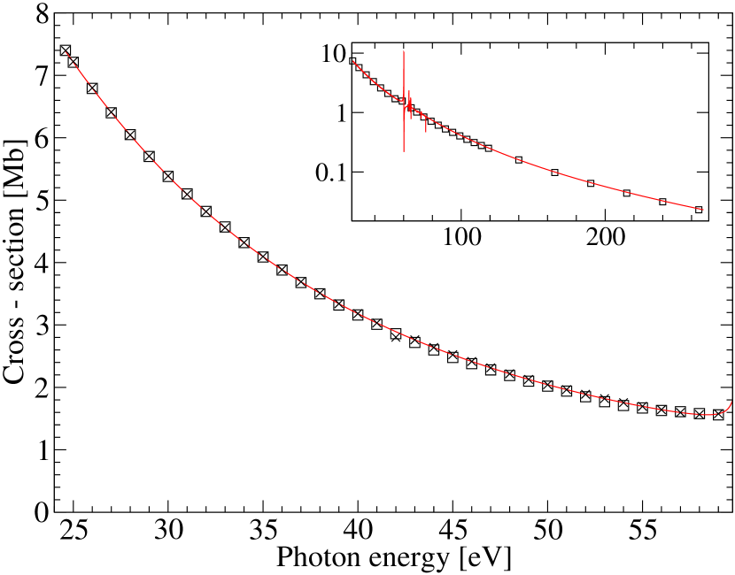
Figure 1: (Colour online) Total photoionisation cross section of helium (¹S ground state) from the ionisation threshold to 59 eV (red ——: present work, $\times$: theoretical values of Venuti et al[6], □: experimental values of Samson et al[1, 2]). The inset shows the theoretical PCS of this work and experimental values of Samson et alon a logarithmic scale for higher photon energies.

In Table 1 the calculated ab initio PCS values are listed for the length and velocity forms of the dipole operator. A remarkable agreement of the order of $10^{-3}\mathrm{Mb}$ can be noticed between these two formulations that for exact wave functions yield identical results. The results are given for the optimal values $\theta_{\mathrm{opt}}$ obtained according to Equation (4). However, overall, only a very small variation of the PCS with $\theta$ is found which indicates that the used basis set is rather complete for the considered energy range.

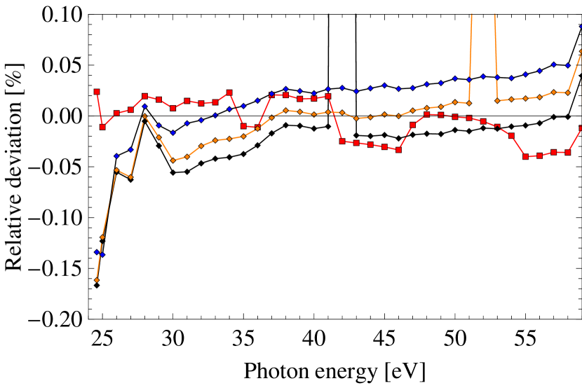
Figure 2: (Colour online) Relative deviation of our results in velocity form (red □) and of the results of Venuti et al[6] (◆) in length (orange), velocity (black), and acceleration forms (blue) from the helium photoionisation cross section calculated in this work within the length formulation.

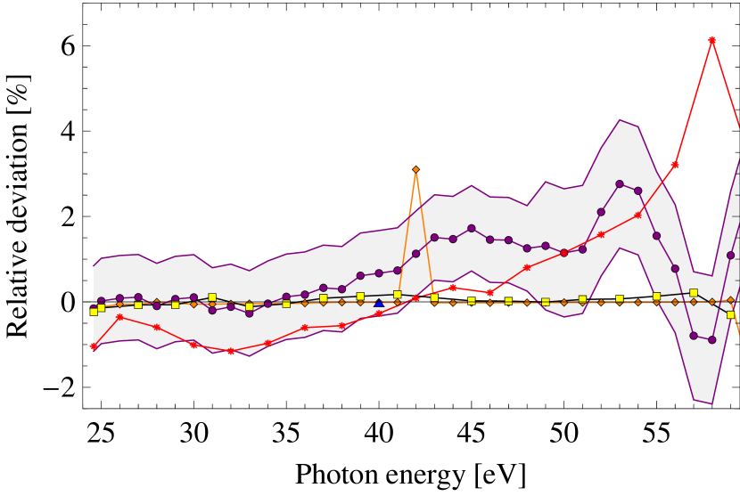
Figure 3: (Colour online) Relative deviation from the helium photoionisation cross section calculated in this work (length form): theoretical data of Venuti et al[6] (orange ◆, length form), Chang and Fang [21] (yellow □, length form), as well as Ivanov and Kheifets (single point at 40 eV, blue △) [8], the experimental values of Samson et al[1, 2] (violet ○), and the compiled data of Yan et al[22] (red $\ast$). The shaded area illustrates the error range estimated by Samson et alfor their experiment ($\pm 1\%$ until 48 eV and $\pm 1.5\%$ starting from 49 eV).

Table 1 also compares the present results with the experimental data of Samson et al[1] and the supposedly most accurate previous calculation of Venuti et al[6]. If shown graphically, as in Figure 1, there are almost no visible differences between the various theoretical and experimental results.

The very good agreement of the present results with the ones in [6] is confirmed in Figure 2 that shows the relative deviation to the present length-form data for photon energies below 59 eV. Despite the completely different theoretical approaches the agreement is remarkably good, since the deviation is less than $0.16\%$ and especially in the energy range from $38\,\mathrm{eV}$ to $58\,\mathrm{eV}$ the relative deviation is of the order of $\pm 0.03\%$ (except for the values in [6] at $42\,\mathrm{eV}$ (length form) and at $52\,\mathrm{eV}$ (velocity form), which we suggest to be typos). Figure 2 shows also the deviation between our results in length and velocity form. Again good agreement with deviations less than $\pm 0.04\%$ is found. In an earlier work, Chang and Fang adopted in [21] a theoretical approach that is practically identical to the one used in [6], but a smaller basis set was used. Our results agree also well with the ones in [21] (relative error of about $0.1\%$), but are consistently in better agreement with the ones in [6]. Clearly, on this level of accuracy convergence of the adopted basis set is finally decisive, while the two completely different approaches ($B$ splines with box discretisation vs. Slater-type orbitals with complex scaling) appear to yield identical results within the achieved level of convergence. This indicates the correct and numerically stable implementation of both approaches. In fact, in the case of the single data point (at 40 eV) given within the energy range shown in Figure 2, the result of the Floquet calculation by Ivanov and Kheifets [8] agrees also within $0.03\%$ with our results and the one in [6]. Therefore, three different theoretical approaches agree within an extremely small relative error.

On the other hand, the experimental helium PCS of Samson et al[1, 2] is still the primary reference for benchmarks and comparison, despite the fact that recent numerical calculations [6, 8] yielded cross sections that differ from the experimental values outside the estimated experimental error bars. In view of the already discussed very good agreement with the theoretical data in [6] (Figure 2), we confirm the deviations to the experimental data in [1, 2] outside the error bars. This can clearly be seen in Figure 3. For photon energies between $51\,\mathrm{eV}$ and $55\,\mathrm{eV}$ the relative deviation of the results of Samson et alfrom our data and also from the ones of Venuti et alis evidently above the error of $\pm 1.5\%$ estimated by Samson et al[1, 2]. The largest deviation of approximately $2.6\,\%$ in comparison to our values occurs at $53\,\mathrm{eV}$ and $54\,\mathrm{eV}$. These deviations are too large to be explained by a failure of the approximations adopted in the present calculation. Neither effects due to the finite size of the nucleus nor relativistic effects should be of a magnitude that is sufficient for explaining such a discrepancy that in addition would have to be strongly photon-energy dependent. As is discussed below on the basis of the derived analytical high-energy tail, also the consideration of non-dipole terms and thus a break-down of the dipole approximation yields corrections that are orders of magnitudes smaller than the ones required to find agreement between theory and experiment.

In view of the in the Introduction discussed importance of the He PCS there exist also data sets that represent a compilation of experimental and theoretical data and try to cover large photon-energy ranges. Such a data set was reported by Yan et al[22] and was claimed by its authors to be reliable for all energies. The comparison in Figure 3 shows that agreement with the here considered theoretical results is reasonable, but not really good. In fact, at both ends of the shown energy range the agreement of the theoretical data with the compiled ones is less good than the one found for the experimental data in [1, 2]. Since the compiled data lie below the theoretical ones for low energies and above for larger energies, the agreement is only good for intermediate energies close to the crossing point at about 42 eV. Especially close to the ionisation threshold the experimental data in [1, 2] appear to be clearly superior to the compiled ones in [22]. In fact, within the first 10 eV above the ionisation threshold the experimental data are in remarkable agreement to theory with a deviation of less than about $0.15\,\%$.

3.2 High-Energy Photoionisation Cross-Section

Table 2: Total photoionisation cross sections $\sigma$ for $\mathrm{He}$ at high photon energies $E$ (in eV). Until $E=250\,$eV the $\sigma$ values are given in Mb and our results stem from the full ab-initio calculation. Starting from 400 eV the results for the model tail (9) are given and all $\sigma$ values are in Barn. Our results are compared to the experimental values of Samson et al[1], the B-spline calculation of Decleva et al[7], and the Floquet results of Ivanov and Kheifets [8].

• 	This work		Decleva et al[7]		Samson et al[1]	Ivanov et al[8]
  $E$	000$\sigma_{l}$	000$\sigma_{v}$	000$\sigma_{l}$	000$\sigma_{v}$	000$\sigma_{\mathrm{exp}}$	000$\sigma_{\mathrm{Fl}}$
  0080	0000.73721	0000.73777	0000.759	0000.74	0000.693	0000.7369
  0085	0000.63041	0000.63099	-—	-—	0000.595	0000.6308
  0091	0000.52708	0000.52762	-—	-—	0000.502	0000.5272
  0095	0000.47011	0000.47063	-—	-—	0000.45	0000.4701
  0100	0000.40960	0000.41004	0000.417	0000.403	0000.393	-—
  0111	0000.30808	0000.30854	-—	-—	0000.3	0000.3082
  0120	0000.24809	0000.24863	0000.251	0000.243	0000.244	-—
  0140	0000.16041	0000.16108	0000.167	0000.158	0000.160	-—
  0160	0000.10924	0000.10985	0000.112	0000.108	0000.108	-—
  0180	0000.07749	0000.07799	0000.802	0000.077	0000.076	-—
  0205	0000.05270	0000.05321	-—	-—	0000.051	0000.0529
  0250	0000.02881	0000.02939	0000.0306	0000.0293	0000.0277	-—
  0400	6561	6812	7270	7009	6370	-—
  0600	1785	1871	2001	1940	1770	-—
  1000	0335	0354	0395	0384	0339	-—
  2000	0033.1	0035.2	0039.5	0040	0034.8	-—
  3000	0008.42	0008.96	-—	-—	0008.77	-—
  4000	0003.17	0003.38	-—	-—	0003.20	-—
  5000	0001.48	0001.58	-—	-—	0001.47	-—
  6000	0000.79	0000.85	-—	-—	0000.77	-—
  7000	0000.47	0000.50	-—	-—	0000.45	-—
  8000	0000.30	0000.32	-—	-—	0000.28	-—

Motivated by the recent work of Ivanov and Kheifets [8] who claim an even larger deviation from the experimental data of Samson et alfor larger photon energies than for the lower ones considered in [6], we also studied the single-photon ionisation process in the non-resonant energy regime above the $\mathrm{He}^{+}$ ionisation threshold ($E\approx 79\,\mathrm{eV}$).

Although our approach, the expansion of the two-electron wave function in Slater-type orbitals, was originally developed for bound-state transitions, the extension by the complex-scaling method provides also an excellent description of high-energy continuum states of the $\mathrm{He}$ atom [9]. Figure 4 shows the deviation of various theoretical, experimental, and compiled data from our results for energies between $80\,\mathrm{eV}$ and $205\,\mathrm{eV}$. The agreement with an older B-spline calculation by Decleva et al[7] is by far not as good as the one found with the later work [6] of the same authors that concentrated on the low-energy regime. However, the deviation of our values from the Floquet results of Ivanov and Kheifets [8] is for most of the data points less or equal to about $0.03\%$. Only at the highest energy, $205\,\mathrm{eV}$, a deviation of $0.37\%$ is found. Therefore, we again confirm the discrepancy between previous theoretical calculations and the experimental reference data of Samson et al, this time reaching to about $6\%$ at $80\,\mathrm{eV}$, as can also be seen from the comparison of the different results in Table 2.

On the other hand, we find in the energy range between about 110 eV and 160 eV a deviation from experiment that remains basically below $2\,\%$. Furthermore, the compiled data of Yan et al[22] agree in this complete energy interval better with the theoretical results than the experimental results of Samson et al, in contrast to the findings at lower photon energies. In the energy interval between about 80 eV and 100 eV the experimental values reported by Bizau and Wuilleumier [23] deviate from our calculation in a qualitatively very similar fashion as the experimental data of Samson et al. However, quantitatively, the deviation is smaller and remains in between 3 and $5\,\%$. In between 100 eV and 150 eV the data in [23] are on the other hand substantially smaller than our theoretical results, leading to a deviation of up to $7\,\%$. For the higher energies shown in Figure 4 the deviation of both experimental data sets from our results is again qualitatively similar, but the ones of Bizau and Wuilleumier lie below our results and approach the latter with increasing energy, while the ones of Samson et allie above and thus agreement with our data becomes worse for increasing photon energy.

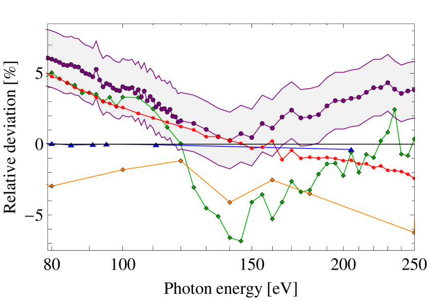
Figure 4: (Colour online) Relative deviation from the helium photoionisation cross section calculated in this work: Floquet calculation of Ivanov and Kheifets [8] (blue △), B-spline calculation of Decleva et al[7] (orange ◆) experimental data measured by Samson et al[1] (violet ○) or Bizau and Wuilleumier [23] (green ◆), and the compiled values by Yan et al[22] (red $\ast$). The shaded area illustrates the error range estimated by Samson et alfor their experiment ($\pm 2\%$).

For very high photon energies above $300\,\mathrm{eV}$ we propose to use the analytical model tail introduced in Equation (9). In order to determine the tail parameter $Z_{i}$, we performed a least-squares fit of the tail to our ab initio calculation in the energy range from $136\,\mathrm{eV}$ to $272\,\mathrm{eV}$ and obtained $Z_{i}=1.5293$. This value lies in between the prediction based on either $Z_{i}=\sqrt{2I}=1.34$ or the mean-field result, $Z_{i}=1.6875$. Although the fit interval spans only a small energy region of the calculated PCS, the extrapolated PCS agrees in a much larger energy range well with the ab-initio results and in the complete shown energy range from 300 eV to $8\,\mathrm{keV}$ very well with the experimental data of Samson et al(Figure 5). In fact, we found almost the same effective initial charge, $Z_{i}=1.53\pm 0.01$, when fitting the tail to the experimental data of Samson et al. The indicated uncertainty arises from different starting points of the energy span at the fitting procedure, while the end point was always chosen at an energy of $8\,\mathrm{keV}$. Figure 6 shows two alternative tails besides the already discussed one. If $Z_{i}$ is fixed to its mean-field value (1.6875) and $Z_{f}$ is used as a fit parameter, the resulting tail lies above the experimental data of Samson et al. While the slope differs for photon energies at about 300 eV, an almost constant off-set is found between the tail and the experimental data for large energies, if plotted on a doubly logarithmic scale. A further off-set is observed, if all tail parameters are fixed on the basis of simple arguments, i. e., the initial charge $Z_{i}$ is set to the mean-field value $1.6875$ and the final charge $Z_{f}$ to the value $1.0$ that should be appropriate at very large separation of the ejected electron. Not shown is the tail that is obtained under the assumption of no relaxation ($Z_{i}=Z_{f}$), since this tail does not agree to the experimental data at all.

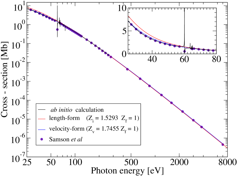
Figure 5: (Colour online) Analytical model tails for different representations of the dipole operator: length-form (red line) and velocity-form (blue line) for their optimal parameters $Z_{i}$ and $Z_{v}$. Also the present ab initio results and the experimental data of Samson et alare plotted. The inset shows the curves on a linear scale for low energies.

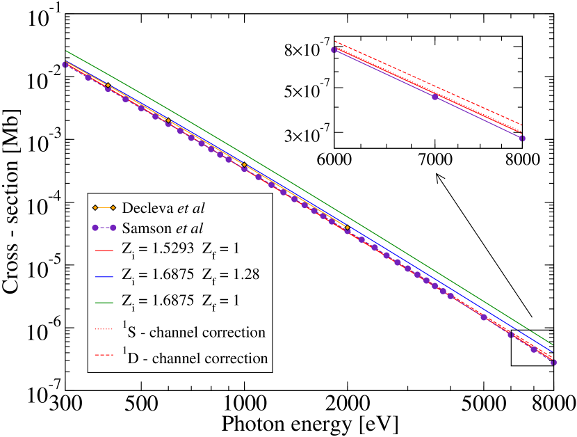
Figure 6: (Colour online) The analytic tail (see Equation (9), solid lines) that is an approximation to the photoionisation cross section of He at high energies is shown for different parameters $Z_{i}$ and $Z_{f}$ (as specified in the graph) and is compared to the experimental values of Samson et al[1] (violet ○) and the calculation of Decleva et al[7] (orange ◆). The dotted and dashed lines show the first-order corrections to the dipole approximation according to Equation (12) due to final states with S or D symmetry, respectively. The inset shows the high-energy part of the spectrum on a linear scale.

Alternatively to the described tail, an asymptotic representation of the cross section is often used as an estimate in the high-energy regime. The asymptotic limit of our length-form model tail is (in atomic units)

$$\tilde{\sigma}_{0}^{L}(E)\approx N\frac{8\sqrt{2}Z_{i}^{3}(Z_{f}-2Z_{i})^{2}}{3\pi}E^{-7/2}$$ (16)

and for the photoionisation of helium we obtain $\tilde{\sigma}_{0}^{\mathrm{He}}(E)\approx 487.956\,E\,(\mathrm{keV})^{-7/2}$. The pre-factor is consistent with the values discussed by Samson et alfor different experimental data. It should be noted, however, that the analytic tail in (9) possesses a much larger validity regime than the asymptotic expression in (16), since it shows good agreement with experiment and ab initio theory already for much lower photon energies.

As mentioned above the length and velocity representations of the dipole operator lead to different expressions for the model tail. However, one may use the different representations to perform a consistency check of our model and to learn about the reliability of the fit procedure. For energies near infinity where the model is surely applicable the representations should lead to equivalent values. Thus we demanded the identity of the length and velocity model tails in the first order of the asymptotic expansion. The asymptotic limit of the model tail in velocity representation is

$$\tilde{\sigma}_{0}^{V}(E)\approx N\frac{8\sqrt{2}Z_{v}^{5}}{3\pi}E^{-7/2}\quad.$$ (17)

Combining (16) and (17) allows to define a fixed relation between $Z_{i}$ and $Z_{v}$ and thus to define a new parameter $Z_{v}^{*}$ that fulfils this relation,

$$Z_{v}^{*}=\left(4Z_{i}^{5}-4Z_{f}Z_{i}^{4}+Z_{f}^{2}Z_{i}^{3}\right)^{1/5}\quad.$$ (18)

For $Z_{i}=1.5293$ and $Z_{f}=1$ this expression leads to $Z_{v}^{*}=1.7224$, while by applying the same fit procedure for $\tilde{\sigma}_{0}^{V}$ as was used before for $\tilde{\sigma}_{0}^{L}$ we find $Z_{v}=1.7455$. Clearly, the differently obtained values for $Z_{v}$ and $Z_{v}^{*}$ are in quite reasonable agreement. Thus we conclude that the model tail, although it is derived with approximate wave functions, yields for very high energies the required independence of the chosen representation (length or velocity form) of the dipole operator. Furthermore, because the results of Equation (18) and the fit are in very good agreement, it is evident that the fit procedure is most suitable to derive the parameter values for the model tail. It may finally be observed that $Z_{v}$ (and $Z_{v}^{*}$) are close to the mean-field value 1.6875. This may indicate that, if one would like to avoid the fit or if no data are available for performing a fit, the best choice for a parameter-free tail is the tail in velocity form adopting the mean-field prediction for $Z_{v}$.

In Figure 5 the length and velocity model tails are plotted for their optimal values. It can be observed that the photon energy where the model tail approaches the ab initio calculation is lower for the velocity form than for the length form. In fact, it is quite surprising how well the velocity-form tail agrees to the full ab-initio results and the experimental data even down to the ionisation threshold. This superiority of the velocity form compared to the length form found at low energies is, however, on the first glance a little bit surprising, since the transition dipole matrix elements in length form are usually supposed to be preferable at low photon energies [8, 24]. This is often explained by the lower sensitivity of the length-form matrix elements to errors in the long-range part of the wavefunctions and the fact that low-energy transitions are more sensitive to this long-range part. However, it may be remembered that the obtained value of $Z_{v}$ is quite close to the mean-field prediction. Since the low-energy part of the photoionisation spectrum is more sensitive to the details of the atomic potential, a model like the velocity-form tail that is closer to the mean-field prediction may thus be favourable compared to the length-form tail with a rather different value found for the corresponding parameter $Z_{i}$.

In order to demonstrate the generality of the analytical tail, we investigated its applicability to other two-electron systems. Besides the neutral helium atom we considered the hydrogen anion, the lithium cation, and even the $\mathrm{HeH}^{\,+}$ molecular cation. The used tail parameters are listed in Table 3. Figure 7 shows a comparison of the tails for these systems with corresponding literature data and, for the atoms, also with ab-initio results calculated in this work. The found agreement is in all cases good or even very good. This indicates the universality of the tail concept. It is, in fact, interesting that the tail works well even for a system like $\mathrm{H}^{-}$ in which the escaping electron experiences within the tail model no influence from the remaining hydrogen atom, since polarisation effects are ignored. Furthermore, the initial state of H^- is only bound due to correlation and thus a mean-field model is in principle not applicable. Nevertheless, also in this case the tail seems to work well. In the case of HeH⁺ a high-energy tail had been proposed before [12], but a paramter-free tail (with $Z_{i}=Z_{f}=\sqrt{2I})$ had been used. The result is also shown in Figure 7. It also compares reasonably well with the full ab-initio results. The reason is that in this case $Z_{i}$ is very close to $Z_{f}$ and, in fact, also to $\sqrt{I}$. Note, for a molecular system there is the additional complication due to nuclear motion. However, in the spirit of the high-energy tail it should have a negligible influence on the high-energy part of the photoionisation spectrum. Therefore, the tail is formally obtained for a single internuclear separation, usually the equilibrium distance. Here, we chose in agreement to [12] the ionisation energy $I=45\,$eV.

Table 3: Parameters for the model tail for various one- and two-electron systems.

• Parameters	$\mathrm{H}^{-}$	H	$\mathrm{He}$	$\mathrm{He}^{+}$	$\mathrm{Li}^{+}$	$\mathrm{HeH}^{+}$
  $Z_{i}$	0.5586	1	1.5293	2	2.5191	1.9414
  $Z_{v}$	0.7662	1	1.7455	2	2.7390	1.9026
  $Z_{v}^{*}$	0.7371	1	1.7224	2	2.7152	1.9177
  $Z_{f}$	0	1	1	2	2	2
  $N$	2	1	2	1	2	2
  $I$ [$\mathrm{eV}$]	0.75436	13.606	24.5912	54.4234	75.64	45

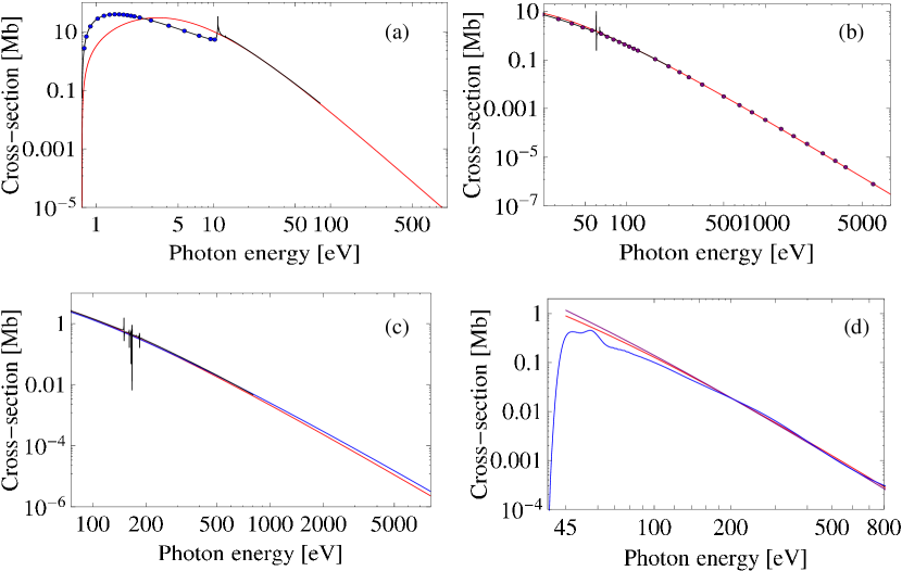
Figure 7: (Colour online) Analytical model tails (length form, red solid lines) for different two-electron systems are compared to literature data. a) $\mathrm{H}^{-}$: Venuti and Decleva [25] (blue ○), b) $\mathrm{He}$: Samson et al[1] (violet ○), c) $\mathrm{Li}^{+}$: Verner et al[26] (blue line), and d) $\mathrm{HeH}^{+}$ (parallel contribution): Saenz [12] (blue line). For the atoms (a to c) also ab-initio cross sections obtained within this work are shown (black solid lines), while for HeH⁺ the alternative tail proposed in [12] is additionally given (purple solid line).

According to (12) the model tail provides the possibility to give an analytical estimate of the first-order correction to the dipole approximation. The two contributions from final states with S and D symmetry are also shown in Figure 6. While the D contribution is clearly dominant, the total correction to the dipole approximation is still negligibly small at photon energies of several keV. Note, however, that the relative contribution reaches already $11\%$ at $8\,\mathrm{keV}$ due to the very small cross section of less than $1\,\mathrm{barn}$. This allows to conclude that very accurate studies of the photoionisation cross section of He performed in the keV photon energy range must take corrections to the dipole approximation into account. However, since the correction is proportional to the squared photon energy and the cross section itself increases by almost five orders of magnitude when going from 8 keV to 300 eV photons, corrections due to a break-down of the dipole approximation are negligible within the here considered level of accuracy for photon energies below 200 eV. Therefore, the deviations between the theoretical results of the present work as well as the ones in [25] or [8] from the experimental reference data of Samson et al[1, 2] or Bizau and Wuilleumier [23] cannot be explained by a failure of the dipole approximation.

4 Summary

An ab initio calculation of the photoionisation cross section of He has been performed for photon energies covering the non-resonant part of the spectrum from the ionisation threshold until about 300 eV. An analytical high-energy model tail has been introduced and the ab initio data were used in order to determine the single fit parameter. With this tail it became possible to predict the photoionisation spectrum for arbitrarily large photon energies within the underlying non-relativistic dipole approximation. Furthermore, the first-order correction to the dipole approximation could be estimated analytically with the aid of the model tail.

Our theoretical results agree extremely well with the ones obtained by different theoretical approaches in the low and the high energy parts by Venuti et al[6] and Ivanov and Kheifets [8], respectively. Therefore, we confirm the pronounced deviation between theoretical and experimental results noted in those earlier works. Particularly, at the photon-energy range around $50\,$eV that is very relevant to present-day FELs like FLASH or high-harmonic sources the relative deviation is unambiguously larger than the error estimates of the experiment of Samson et al[1, 2]. Since we also demonstrated the validity of the dipole approximation at least for photon energies up to 200 eV where the previous comparisons were performed, this possible source of disagreement between theory and experiment is excluded. We thus conclude that the quality of theoretical calculations of the helium photoionisation cross section has reached a consistently higher level than the experiment. In view of the fundamental importance of the photoionisation cross section of helium we hope that the present work stimulates future experimental efforts to resolve the discrepancies between theory and experiment. Until this has been achieved, we propose to use the theoretical results, especially the ones of the present work that cover a large photon energy range in a consistent fashion, instead of the experimental ones as reference data for, e. g., calibrating new light sources, since they appear to be more accurate and reliable.

References

References

- [1] Samson J A R, He Z X, Yin L and Haddad G N 1994 J. Phys. B 27 887
- [2] Samson J A R and Stolte W C 2002 J. Electr. Spectros. Relat. Phenom. 123 265
- [3] Wellhöfer M, Hoeft J T, Martins M, Wurth W, Braune M, Viefhaus J, Tiedtke K and Richter M 2008 3 P02003
- [4] Nagasono M, Suljoti E, Pietzsch A, Hennies F, Wellhöfer M, Hoeft J T, Martins M, Wurth W, Treusch R, Feldhaus J, Schneider J R and Föhlisch A 2007 Phys. Rev. A 75 051406
- [5] Mitzner R, Sorokin A A, Siemer B, Roling S, Rutkowski M, Zacharias H, Neeb M, Noll T, Siewert F, Eberhardt W, Richter M, Juranic P, Tiedtke K and Feldhaus J 2009 Phys. Rev. A 80 025402
- [6] Venuti M, Decleva P and Lisini A 1996 J. Phys. B 29 5315
- [7] Decleva P, Lisini A and Venuti M 1994 J. Phys. B 27 4867
- [8] Ivanov I A and Kheifets A S 2006 Eur. Phys. J. D 38 471
- [9] Stark A and Saenz A 2010 Phys. Rev. A 81 032501
- [10] Fano U and Cooper J W 1968 Rev. Mod. Phys. 40 441
- [11] Rescigno T N and McKoy V 1975 Phys. Rev. A 12 522
- [12] Saenz A 2003 Phys. Rev. A 67 033409
- [13] Saenz A, Weyrich W and Froelich P 1993 Int. J. Quant. Chem. 46 365
- [14] Barbieri R S and Bonham R A 1991 Phys. Rev. A 44 7361
- [15] Saenz A and Froelich P 1997 Phys. Rev. C 56 2162
- [16] Bethe H A and Salpeter E E 1977 Quantum Mechanics of One- and Two-Electron Atoms (New York: Plenum)
- [17] Saenz A 2000 J. Phys. B 33 4365
- [18] Saenz A 2000 Phys. Rev. A 61 051402(R)
- [19] Lühr A, Vanne Y V and Saenz A 2008 Phys. Rev. A 78 042510
- [20] Wang S 1999 Phys. Rev. A 60 262
- [21] Chang T N and Fang T K 1995 Phys. Rev. A 52 2638
- [22] Yan M, Sadeghpour H R and Dalgarno A 1998 Astrophys. J. 496 1044
- [23] Bizau J M and Wuilleumier F J 1995 J. Electr. Spectros. Relat. Phenom. 71 205
- [24] Johnston R R 1964 Phys. Rev. 136 A958
- [25] Venuti M and Decleva P 1997 J. Phys. B 30 4839
- [26] Verner D A, Ferland G J, Korista K T and Yakovlev D G 1996 Astrophys. J. 465 487