Inferring the eccentricity distribution

Abstract

Standard maximum-likelihood estimators for binary-star and exoplanet eccentricities are biased high, in the sense that the estimated eccentricity tends to be larger than the true eccentricity. As with most non-trivial observables, a simple histogram of estimated eccentricities is not a good estimate of the true eccentricity distribution. Here we develop and test a hierarchical probabilistic method for performing the relevant meta-analysis, that is, inferring the true eccentricity distribution, taking as input the likelihood functions for the individual-star eccentricities, or samplings of the posterior probability distributions for the eccentricities (under a given, uninformative prior). The method is a simple implementation of a hierarchical Bayesian model; it can also be seen as a kind of heteroscedastic deconvolution. It can be applied to any quantity measured with finite precision—other orbital parameters, or indeed any astronomical measurements of any kind, including magnitudes, distances, or photometric redshifts—so long as the measurements have been communicated as a likelihood function or a posterior sampling.

Section 1 Introduction

With rare exceptions, binary star and exoplanet science hinges not on the specific value of any individual eccentricity (or mass or period), but rather on the distribution, or the distribution as a function of stellar properties or other parameters. The goal of any statistical study should be to determine the distribution of the quantity of interest—we will concentrate on orbital eccentricity for specificity—that would have been observed if the investigator had extremely high signal-to-noise data and some (magical) method for precise determination of all nuisance parameters, such as instrument calibration and system inclination and so forth. That is, the investigator wants the observational-uncertainty-deconvolved distribution of the quantity of interest.

One exciting development in the study of binaries and exoplanets is that many groups are building probabilistic modeling software (Ford 2005; Gregory 2005; Balan & Lahav 2009). Rather than fitting and returning a single set of parameters, These probabilistic packages (approximately) sample from the posterior probability distribution under weak-prior assumptions. These posterior samplings are much more useful than best-fit parameter values, because they permit subsequent investigators to perform probabilistic inference on the output without going back to the raw radial-velocity data while still properly propagating uncertainties. In this Article, we give an example of probabilistic meta-analysis that becomes possible when the parameter outputs for individual stars are probabilistic.

For any plausibly exoplanet- or binary-hosting star $n$, there are parameters

$$\displaystyle\boldsymbol{\omega}_{n} \equiv \left(\kappa_{n},T_{n},\phi_{n},e_{n},\varpi_{n}\right)\quad,$$ (1)

where $\kappa_{n}$ is the velocity amplitude, $T_{n}$ is the period, $\phi_{n}$ is some orbital phase or fiducial time, $e_{n}$ is the eccentricity, and $\varpi_{n}$ is the longitude of perihelion. Fitting to these parameters is non-linear and unbiased estimators are rare. For these reasons, maximum-likelihood (or, for Gaussian noise, minimum-$\chi^{2}$) parameters are not in general unbiased estimators of the true parameters—maximum-likelihood estimators only become unbiased in the limit of an infinite amount of data. Almost all single-point estimates, including maximum-a-posteriori or median-of-sampling parameters, are also biased in general (Lehmann & Casella 1998).

Indeed, along these lines, it has been shown that the eccentricity $e_{n}$ of any star $n$ has this property: The maximum-likelihood estimate $\tilde{e}_{n}$ of the eccentricity is biased high; any histogram of estimated eccentricities $\tilde{e}_{n}$ will have a mean (and variance) that is higher than that of the true distribution of true eccentricities $e_{n}$ (Shen & Turner 2008). These results—and the incredible diversity of eccentricities observed in exoplanet systems—motivate a concentration on the eccentricity distribution in what follows. Without the analysis methods we propose here, it is possible that conclusions about the high eccentricities of exoplanet systems might be over-stated or distorted.

There are three fundamental approaches to determination of the true eccentricity distribution—or true distribution of any quantity—given noisy measurements $\tilde{e}_{n}$, where $n$ is an index over instances (in this case, stars with binary or exoplanet companions). The first (and worst) is just to adopt the estimated values as good estimates of the true values and create a histogram (or other density estimate) of the observed values $\tilde{e}_{n}$. Because these estimators are biased, and because they are noisy, the distribution created in this way will have the wrong mean and variance; it will be a strongly biased estimate of the true distribution of true eccentricities $e_{n}$. Furthermore, adding new $\tilde{e}_{n}$ estimates from new stars $n$ will not decrease these biases; there is no $\sqrt{N}$ improvement as new data are added. There are suggestions of less-biased estimators for eccentricity (Zakamska et al 2010), but anything unbiased in eccentricity $e$ will still be biased for any nonlinear function of $e$, and point estimates still have the property that the distribution of point estimates will in general be different in variance from the true distribution, if only because of observational noise.

The second approach is to deconvolve the distribution of maximum-likelihood or best-fit $\tilde{e}_{n}$ values. In this approach the investigator recognizes that the distribution of estimates $\tilde{e}_{n}$ is the true distribution convolved with the uncertainty distribution, where that uncertainty can be described as the probability of estimating $\tilde{e}_{n}$ when the true value is $e_{n}$, or $p(\tilde{e}_{n}|e_{n})$. The investigator finds the distribution of true values $e_{n}$ that, when it is convolved with the uncertainties, produces the distribution of estimates $\tilde{e}_{n}$. Done correctly, this will be performed in a forward-modeling of the observed distribution, starting at the true distribution. This method is much more responsible, but when the investigator works at the distribution level (that is, not at the individual-star level), the investigator must assume things about the distribution of uncertainties, equivalent to assuming that all the stars have the same relationship $p(\tilde{e}_{n}|e_{n})$ between the estimated and true values. It is also a disadvantage that when performed naïvely, deconvolutions can be very sensitive to histogram binning (or, equivalently, choices about the density estimation) and are unstable to “ringing” and other issues coming from shot noise in the observed distribution.

The third approach—and the approach taken here—is forward modeling of the heteroscedastic observed data (or eccentricity estimates, if these estimates are not single point estimates but rather posterior samplings). That is, the investigator makes a non-parametric (or highly parameterized) model of the frequency distribution function ${f_{\boldsymbol{\alpha}}}(e)$ for the true $e_{n}$ values, and finds the best-fit values of the distribution parameters $\boldsymbol{\alpha}$—the values of the parameters $\boldsymbol{\alpha}$ that, after convolution with the (suitably transformed) distributions in the nuisance parameters, explains best the full set of eccentricity samplings. This is also essentially deconvolution, but it has the enormous advantage over naïve deconvolution that it accounts for the fact that different stars have different levels of (and functional forms for) uncertainty in the nuisance parameters. This forward-modeling approach is slowly being adopted in astrophysics (an early proponent is Loredo 2004); we used a simple version of it to estimate the galaxy luminosity function (Blanton et al 2003) and the velocity distribution in the Galaxy disk (Bovy et al 2009a), and we built a general tool for situations in which distributions are smooth and observational uncertainties are simple (Bovy et al 2009b).

Here we perform this forward modeling for a situation in which the observational uncertainties are not simple (uncertainties are asymmetric; measurements are biased) in an area (exoplanet eccentricities) of great current scientific interest. Everything that follows is straightforwardly generalized to other parameters and other kinds of systems. For example, parallax-based stellar distances, photometric redshifts, and faint-source fluxes also suffer from systematic biases (Lutz & Kelker 1973; Connolly et al 1995; Hogg & Turner 1998). Scientific results based on these measurements rely on the true distributions, not the distributions of (biased) measurements, and in all of these cases, the objects of greatest interest have measurements at relatively low precision or low signal-to-noise. Reliable scientific results can be obtained nonetheless, though only by modeling the data; that is the fundamental motivation for this work.

Section 2 Method

There are $N$ stars $n$ ($1\leq n\leq N$), each of which has some number $M_{n}$ of radial velocity measurements $v_{nj}$. For each star $n$, the set of measurements (data)

$$\displaystyle\boldsymbol{D}_{n} \equiv \left\{{v_{nj}}\right\}_{j=1}^{M_{n}}$$ (2)

is modeled as being affected by a single companion. We are not explicitly considering multiple companion stars or planets at this stage, although the generalization is straightforward. The model is

$$\displaystyle v_{nj} = V_{n}+g_{n}(t_{nj})+E_{nj}\quad,$$ (3)

where $V_{n}$ is an overall system velocity, the function $g(t_{nj})$ is the radial velocity equation, and the $E_{nj}$ are noise contributions drawn from a Gaussian of zero mean and variance $[\sigma_{nj}^{2}+S_{n}^{2}]$, where $\sigma_{nj}^{2}$ is the uncertainty variance for the $j$th observation of star $n$ and $S_{n}^{2}$ is a noise variance from intrinsic stellar variability and other unmodeled sources of noise. The radial velocity equation $g_{n}(t)$ for star $n$ is parameterized by velocity amplitude $\kappa_{n}$, period $T_{n}$, orbital phase $\phi_{n}$, eccentricity $e_{n}$, and longitude of perihelion $\varpi_{n}$. (five parameters). This model of one star has 7 parameters ($V_{n}$, $S_{n}$, and five orbit parameters per star), which we can think of as living in a list ${\boldsymbol{\omega}_{n}}$, and the model of al $N$ stars has $[7\,N]$ continuous parameters in a bigger list $\left\{{{\boldsymbol{\omega}_{n}}}\right\}_{n=1}^{N}$.

The likelihood $\mathscr{L}_{n}$ for the seven parameters ${\boldsymbol{\omega}_{n}}$ for star $n$ is just the probability of the data $\boldsymbol{D}_{n}$ for star $n$ given the parameters ${\boldsymbol{\omega}_{n}}$ for star $n$

$$\displaystyle\mathscr{L}_{n} \equiv p(\boldsymbol{D}_{n}|{\boldsymbol{\omega}_{n}})$$

$$-2\,\ln\mathscr{L}_{n} = Q+\sum_{j=1}^{M_{n}}\ln(\sigma_{nj}^{2}+S_{n}^{2})+\sum_{j=1}^{M_{n}}\frac{\left[V_{n}+g_{\boldsymbol{\omega}_{n}}(t_{nj})-v_{nj}\right]^{2}}{\sigma_{nj}^{2}+S_{n}^{2}}\quad,$$ (4)

where $Q$ is some constant. This looks like $\chi^{2}$ but is modified for the jitter parameter $S_{n}^{2}$.

For each system $n$ we imagine that we have been provided (by the exoplanet observing or fitting team, say) not the original data, but just a $K$-element sample from a posterior probability distribution function (posterior PDF) created from the likelihood and an uninformative prior PDF $p_{0}({\boldsymbol{\omega}_{n}})$:

$$\displaystyle p({\boldsymbol{\omega}_{n}}|\boldsymbol{D}_{n}) = \frac{1}{Z_{n}}\,p(\boldsymbol{D}_{n}|{\boldsymbol{\omega}_{n}})\,p_{0}({\boldsymbol{\omega}_{n}})\quad,$$ (5)

where $Z_{n}$ is a normalization constant (for our purposes). The prior PDF $p_{0}({\boldsymbol{\omega}_{n}})$ will be decided not by us but by the exoplanet-fitter; we expect (need) it to be uninformative, for example, flat in all parameters, or in their logarithms. For each star $n$ this sampling takes the form of a chain of $K$ samples $k$, each of which is a set of 7 parameters ${\boldsymbol{\omega}_{n}}_{k}$, such that the distribution of the samples is consistent with a random draw from the posterior PDF.

The total likelihood $\mathscr{L}$ for all the parameters of all the stars $n$ is just the product of the individual-star likelihoods

$$\displaystyle\mathscr{L} \equiv p(\left\{{\boldsymbol{D}_{n}}\right\}_{n=1}^{N}|\left\{{{\boldsymbol{\omega}_{n}}}\right\}_{n=1}^{N})$$ (6)

$$= \prod_{n=1}^{N}\mathscr{L}_{n}\quad.$$

This product formulation of the total likelihood makes the implicit assumption that the different star observations are independent; that is, we are assuming that there are no likelihood covariances among the parameters of different systems $n$. That assumption will be at least weakly violated in any real survey of binaries or exoplanets, because different observations will share hardware issues and calibration information.

We want, however, not the likelihood for all the star and orbital parameters but instead the likelihood $\mathscr{L}_{\boldsymbol{\alpha}}$ for the parameters $\boldsymbol{\alpha}$ of the eccentricity distribution ${f_{\boldsymbol{\alpha}}}(e)$. This requires a slight re-thinking, because once we know the true eccentricity distribution, that is a better prior PDF to be using than the uninformative prior PDF $p_{0}({\boldsymbol{\omega}_{n}})$. It is this process—opening up the prior PDF to modeling and putting what we want to infer in the place of the prior PDF from previous inferences—that makes the method hierarchical. To make this inference we must change variables and integrate out the individual-star parameters which are—for our purposes—nuisance parameters. For the likelihood function $\mathscr{L}_{\boldsymbol{\alpha}}$, this change of variables and integration is

$$\displaystyle\mathscr{L}_{\boldsymbol{\alpha}} \equiv p(\left\{{\boldsymbol{D}_{n}}\right\}_{n=1}^{N}|\boldsymbol{\alpha})$$

$$\mathscr{L}_{\boldsymbol{\alpha}} = \prod_{n=1}^{N}\int\mathrm{d}{\boldsymbol{\omega}_{n}}\,p(\boldsymbol{D}_{n}|{\boldsymbol{\omega}_{n}})\,p({\boldsymbol{\omega}_{n}}|\boldsymbol{\alpha})$$

$$p({\boldsymbol{\omega}_{n}}|\boldsymbol{\alpha}) \equiv \frac{{f_{\boldsymbol{\alpha}}}(e_{n})\,p_{0}({\boldsymbol{\omega}_{n}})}{p_{0}(e_{n})}\quad,$$ (7)

where the integrals are over the $N$ 7-dimensional parameter spaces and we have multiplied the uninfomative prior PDF $p_{0}({\boldsymbol{\omega}_{n}})$ by a ratio of the eccentricity distribution we want to infer to its uninformative counterpart. This is a marginalized likelihood (or “marginal likelihood”) because we have inserted a prior PDF for the nuisance parameters and integrated them out, but left the result in the dimensions of likelihood (probability of data given parameters).

In multiplying the prior PDF by ${f_{\boldsymbol{\alpha}}}(e)/p_{0}(e)$ we have implicitly assumed that the true distribution of parameters is separable; that is, that both the uninformative prior PDF and the informative prior PDF parameterized by $\boldsymbol{\alpha}$ can be written as a prior PDF on the eccentricity $e$ multiplied by a prior PDF on the other parameters. This is not true in general, and is a limitation of this formulation. The limitation is not fundamental; ${f_{\boldsymbol{\alpha}}}(e)$ can be replaced with a multivariate distribution function in the general case.

The $[7\,N]$-dimensional integral (or product of $N$ 7-dimensional integrals) looks intimidating, but that integration is exactly the capability that the sampling from each individual system $n$ provides for us: Given a $K$-element sampling with elements ${\boldsymbol{\omega}_{n}}_{k}$,

$$\displaystyle\int\mathrm{d}{\boldsymbol{\omega}_{n}}\,p_{0}({\boldsymbol{\omega}_{n}}|\boldsymbol{D}_{n})\,F({\boldsymbol{\omega}_{n}}) \approx \frac{1}{K}\,\sum_{k=1}^{K}F({\boldsymbol{\omega}_{n}}_{k})\quad;$$ (8)

where $p_{0}()$ represents the posterior PDF under the uninformative prior PDF upon which the sampling is based. The point is that all probability integrals can be approximated as sums over samples. So the sampling approximation to the marginalized likelihood for the $\boldsymbol{\alpha}$ is just

$$\displaystyle\mathscr{L}_{\boldsymbol{\alpha}} \approx \prod_{n=1}^{N}\frac{1}{K}\,\sum_{k=1}^{K}\frac{{f_{\boldsymbol{\alpha}}}(e_{nk})}{p_{0}(e_{nk})}\quad,$$ (9)

where all that is inside the sum is the ratio between the uninformative prior PDF (on which the sampling is based) and the new prior PDF that we want to infer, and the $e_{nk}$ are the $K$ samples of each $e_{n}$. This sampling approximation to the likelihood $\mathscr{L}_{\boldsymbol{\alpha}}$ for the parameters $\boldsymbol{\alpha}$ can be optimized to obtain a maximum-likelihood true eccentricity distribution, or it can be multiplied by a prior PDF, normalized, and sampled to obtain a posterior PDF sampling for the parameters $\boldsymbol{\alpha}$. Either way, it is the likelihood that non-trivially enters into our inference.

The expression for the likelihood $\mathscr{L}_{\boldsymbol{\alpha}}$ in equation (9) is an importance-sampling approximation to the ratio of Bayes factors (integrals of the posterior probability distribution over the nuisance parameters). The comparison of marginalized likelihoods of two models (between the default prior PDF and the distribution parameterized by $\boldsymbol{\alpha}$ or between two different values of the parameters $\boldsymbol{\alpha}$) is equivalent to a marginalized Bayesian comparison between two models. It is an importance sampling because it uses a sampling but re-weights the samples by the ratio of probabilities between the two models. The usual caveats concerning importance sampling apply here as well: Since the samples returned by the MCMC are generally not independent, the importance-sampling approximation does not improve as $\sqrt{N}$ and if the default prior PDF and the distribution parameterized by $\boldsymbol{\alpha}$ are very different, the importance-sampling approximation will be noisy. Therefore, we prefer the default prior PDF to be uninformative. We also need it to be uninformative to ensure that the posterior PDF generated with $p_{0}(e)$ has support—and samples—wherever the posterior PDF generated with ${f_{\boldsymbol{\alpha}}}(e)$ is significant.

From an inference perspective, it is more sensible to simultaneously infer $\boldsymbol{\alpha}$ and all the ${\boldsymbol{\omega}_{n}}$ for all the systems, and perform the marginalization on the joint inference. Here we use this importance-sampling approximation because by assumption we do not have the exoplanet data; we have only the $K$-element samplings from the posterior PDFs (the posterior PDFs created with the uninformative prior PDF).

All that remains is to choose functional forms for (parameterizations of) the eccentricity distribution function ${f_{\boldsymbol{\alpha}}}(e)$, and a prior PDF on the parameters $\boldsymbol{\alpha}$ (if we want to perform sampling or further marginalization, which we do). There are many possible choices here, and a true Bayesian doesn’t choose but rather does them all and includes them all in the output. However, for specificity and clarity, we consider only two forms for the eccentricity distribution. The first is a step function with $M$ steps:

$$\displaystyle{f_{\boldsymbol{\alpha}}}(e) \equiv \sum_{m=1}^{M}\exp(\alpha_{m})\,{\textstyle s(e;\frac{m-1}{M},\frac{m}{M})}$$

$$s(x;L,H) \equiv \left\{\begin{array}[]{cl}0&\quad\mbox{for}~{}x<L\\ (H-L)^{-1}&\quad\mbox{for}~{}L\leq x\leq H\\ 0&\quad\mbox{for}~{}H<x\\ \end{array}\right.$$ (13)

$$\sum_{m=1}^{M}\exp\alpha_{m} = 1\quad,$$ (14)

where we have laboriously defined the step function as a mixture of top-hats and given the normalization constraint on the elements $\alpha_{m}$ of the parameter vector $\boldsymbol{\alpha}$. For the prior PDF on the $\boldsymbol{\alpha}$ we use

$$\displaystyle p(\boldsymbol{\alpha}) \propto \delta(1-\sum_{m=1}^{M}\exp\alpha_{m})\,\exp(-\frac{1}{2}\,\epsilon\,\sum_{m=2}^{M}[\alpha_{m}-\alpha_{m-1}]^{2})\quad,$$ (15)

where the delta function ensures the normalization of ${f_{\boldsymbol{\alpha}}}(e)$, and $\epsilon$ is a control parameter that controls our expectation that ${f_{\boldsymbol{\alpha}}}(e)$ be smooth. Of course this smoothness parameter $\epsilon$—and the bin number $M$—should be learned along with $\boldsymbol{\alpha}$, but as this is beyond our scope, we simply set $\epsilon=2$ and $M=20$. Empirically, this keeps the distributions smooth when the data sets get small, but permits good freedom and doesn’t influence the results much for large data sets, as we show below. This is a simple smoothness prior (Kitagawa & Gersch 1996); more sophisticated versions can employ a Gaussian process (Rasmussen & Williams 2006) on the $\alpha_{m}$—the prior in equation (15) is a special case of this—and the hyper-parameters (only $\epsilon$ in this case) controlling the smoothness of the distribution can be marginalized out. This has the advantage that the number of bins can be very large, but it has the disadvantage that sampling highly correlated bin heights is challenging (Murray et al 2010a, b).

The second form we consider for the eccentricity distribution is that of the beta distribution

$$\displaystyle{f_{\boldsymbol{\alpha}}}(e) = \frac{\Gamma(a+b)}{\Gamma(a)\,\Gamma(b)}\,e^{[a-1]}\,(1-e)^{[b-1]}$$

$$\boldsymbol{\alpha} \equiv (a,b)\quad,$$ (16)

where $\Gamma(z)$ is the gamma function, and we are redefining the parameter list $\boldsymbol{\alpha}$ to contain the beta distribution shape parameters $a$ and $b$. This distribution is defined on the interval $0<e<1$ and has remarkable freedom with only two parameters. We take the prior PDF on the parameters $(a,b)$ to be flat in the allowed region $a>0$ and $b>0$. Technically this prior PDF is improper, but the posterior PDF under any realistic data set is proper.

In either case—step function or beta distribution—when we have a set of $J$ samples $\boldsymbol{\alpha}_{j}$ of the distribution-function parameter vector that are effectively samples from the posterior probability distribution, we can use that distribution of distributions or else marginalize out the parameters. The marginalized distribution $\left<{f_{\boldsymbol{\alpha}}}(e)\right>$ is given by

$$\displaystyle\left<{f_{\boldsymbol{\alpha}}}(e)\right>=\frac{1}{J}\,\sum_{j=1}^{J}{f_{\boldsymbol{\alpha}}}_{j}(e)\quad,$$ (17)

where by “${f_{\boldsymbol{\alpha}}}_{j}(e)$” we mean the distribution ${f_{\boldsymbol{\alpha}}}(e)$ made using parameters $\boldsymbol{\alpha}_{j}$ of the $j$th posterior sample.

Section 3 Experiments

We generated $N=400$ ersatz radial velocity data sets $n$, each of which contained $M_{n}=30$ radial velocity measurements scattered uniformly over a time baseline of 1000 days. These measurements were created using the model for the radial velocity of the parent star of a theoretical exoplanet (or companion star in a binary system) described by equation (3). We assumed reasonable distributions for the governing parameters of the model, together with some (trivial) simplifications:

Each ersatz parent or primary star was assumed to have a mass of $M_{n}=1\,M_{\sun}$ and vanishing overall system velocity ($V_{n}=0$) in the absence of its exoplanet (or stellar companion). Intrinsic radial velocity and primary star mass were, though, left free in fitting. Each ersatz exoplanet or companion star was assigned a mass $m_{n}$ drawn from a distribution $p(m)\propto 1/m$ (flat in $\ln m$) constrained to lie in $[0.1\,M_{\mathrm{Jup}}]<m_{n}<[10\,M_{\mathrm{Jup}}]$. Companions were given orbital periods drawn from a distribution $p(T)\propto 1/T$ constrained to lie in $[2\,\mathrm{d}]<T<[2000\,\mathrm{d}]$. Phases $\phi_{n}$ and $\varpi_{n}$ were drawn from uniform distributions $0<\phi<2\pi$, except for the inclination $i_{n}$, which was drawn from a distribution flat in $\cos i$. The masses $M_{n}$ and $m_{n}$ and inclinations $i_{n}$ enter into the radial velocity model through the $\kappa_{n}$:

$$\displaystyle\kappa_{n} = \frac{[2\pi\,G]^{1/3}\,m_{n}\,\sin i_{n}}{T_{n}^{1/3}\,[M_{n}+m_{n}]^{2/3}\,[1-e_{n}^{2}]^{1/2}}\quad.$$ (18)

The eccentricity $e_{n}$ for each ersatz companion was drawn from one of two frequency distributions: The first is an intuitive distribution

$$\displaystyle f(e)=\frac{1}{Z}\left[\frac{1}{[1+e]^{4}}-\frac{e}{2^{4}}\right]$$ (19)

(Shen & Turner 2008), where $Z$ is a normalization constant; hereafter we call this distribution “ST4”. The second is an unrealistic straw-man designed to stress-test the inference methodology. It is a Gaussian with mean $e=0.3$ and variance $(0.05)^{2}$ (but set to zero outside of the range $0<e<1$).

The error added to each ersatz measurement was drawn from a Gaussian of known observational noise variance, but with every point assigned its own individual (heteroscedastic) noise variance, uniformly distributed (in variance) in the interval $(\sqrt{10}~{}\mathrm{m}\,\mathrm{s}^{-1})^{2}<\sigma_{nj}^{2}<(10~{}\mathrm{m}\,\mathrm{s}^{-1})^{2}$. For the ersatz observations, the jitter parameters $S_{n}^{2}$ were set to vanish, but, as with the system velocity and mass of the parent (or primary) star, the jitter parameters $S_{n}^{2}$ were left free in the fitting.

We optimized, fit, and marginalized the radial velocity model to each of the ersatz data sets using Metropolis-Hastings Markov Chain Monte Carlo (MCMC) sampling. For the MCMC we adopted a standard uninformative prior PDF that is flat in $\ln\kappa_{n}$, flat in $\ln T_{n}$, flat in $\phi_{n}$, flat in $\varpi_{n}$, and flat in $e_{n}$. We performed the sampling not in the naive parameter space $(\ln\kappa_{n},\ln T_{n},\phi_{n},e_{n},\varpi_{n})$ but in a better-behaved sampling space of

$$\displaystyle(\ln T_{n},\kappa_{n}\,\cos[\phi_{n}+\varpi_{n}],\kappa_{n}\,\sin[\phi_{n}+\varpi_{n}],e_{n}\,\cos\varpi_{n},e_{n}\,\sin\varpi_{n})\quad.$$ (20)

In this space, sampling is better behaved, but the “natural prior” PDF is not flat in $\ln\kappa_{n}$ or $e_{n}$, so a compensating prior PDF (or Jacobian) must be multiplied in. We confirmed that our sampler is using the correct uninformative prior PDF by running it on empty data sets; the resulting no-data samplings are samplings of the prior PDF.

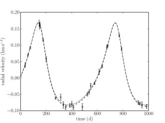
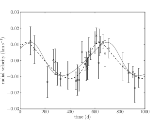
On each system $n$ we set parameter step-sizes (for a Gaussian proposal distribution in the sampling space) such that acceptance ratios were near $0.4$. On each system $10^{6}$ links of MCMC were run, checked for mixing (convergence), and thinned (subsampled uniformly) to produce a set of $K=10^{5}$ nearly independent parameter samples ${\boldsymbol{\omega}_{n}}_{k}$—independence is however not required for the sampling approximation of equation (9) to work. Radial velocity curves for two ersatz exoplanets are shown in Figure 1, together with their MCMC samplings in period and eccentricity. For each system $n$ we search the chain for the maximum-a-posteriori parameters. We also used a modified (simulated annealing) MCMC sampling to find the maximum-likelihood parameters $\tilde{{\boldsymbol{\omega}_{n}}}$, one member of which is the “best-fit” eccentricity $\tilde{e}_{n}$.

At this point we have the full $N\times K$ sampling $e_{nk}$. This makes it possible to compute the marginalized likelihood of equation (9) for any parameters $\boldsymbol{\alpha}$. Again, we perform Metropolis-Hastings MCMC, but now in the space of $\boldsymbol{\alpha}$ with the prior PDF of equation (15). The proposal distribution used in the MCMC was a small Gaussian perturbation applied to every component of $\boldsymbol{\alpha}$, with Gaussian variance chosen to keep the acceptance ratio near 0.4. For each experiment $10^{4}$ links of MCMC were run, and checked for mixing. From this posterior sampling, we can obtain whatever results are desired, the maximum-a-posteriori distribution, the marginalized (mean-of-posterior) distribution, a sampling of distributions consistent with the data, or any quantile of the eccentricity distribution.

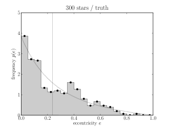
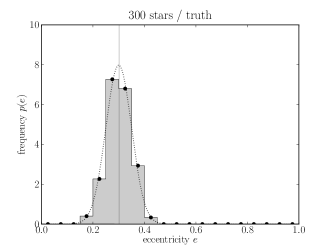
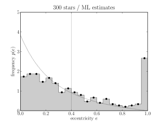
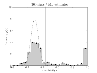
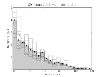
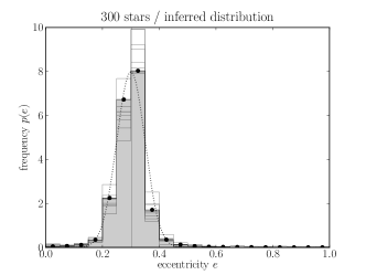
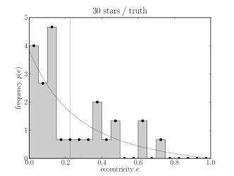
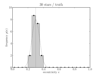
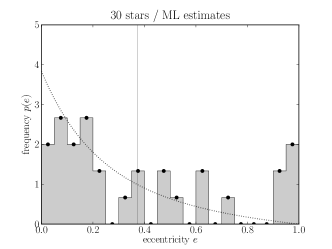
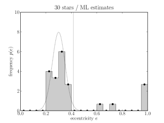
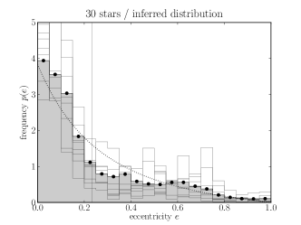
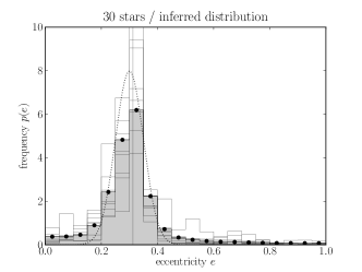
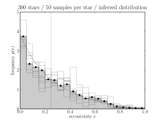
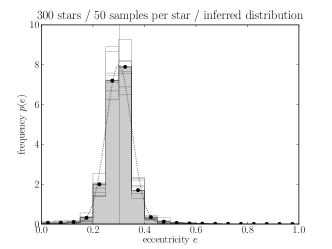
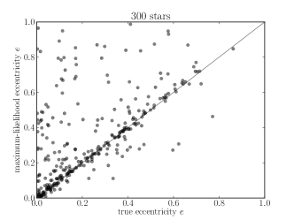
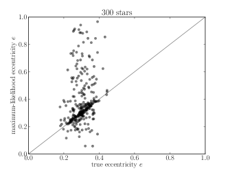
In Figure 2 and Figure 3 we show the results of four experiments, two with $N=300$ systems and two with $N=30$, and two with the ST4 input eccentricity distribution, and two with the Gaussian input eccentricity distribution. We show the true (input) eccentricities, the maximum-likelihood eccentricities, and the inferred distribution. In each case, we find—as expected—that the marginalized (mean-of-posterior) inferred eccentricity distribution is a far better description of the original input eccentricity distribution than the naive distribution created by histogramming the maximum-likelihood eccentricity estimates $\tilde{e}_{n}$. The inferred distribution captures well the smooth distribution that was used to generate the ersatz data. Furthermore, where the actual finite sampling of true values departs (just by Poisson statistics) from the smooth distribution, the inferred distribution even captures those deviations, especially when there are $N=300$ systems (Figure 2).

Figure 2 and Figure 3 also show that the mean of the eccentricity distribution is over-estimated when the best-fit eccentricities $\tilde{e}_{n}$ are used to represent the eccentricity distribution, and that the over-estimate does not decrease as the number of objects increases. However, the marginalized inferred mean—the mean obtained by marginalizing over samples—is a very good estimate of the true mean of the true distribution. The same holds for all of the quantiles of the distribution.

The sampling in $\boldsymbol{\alpha}$ provides full uncertainty information, including the uncertainty in every component of $\boldsymbol{\alpha}$ and also all of the component–component covariances. In Figure 2 and Figure 3 we show only a superimposed sampling. This conveys information about the uncertainty distribution in each bin, but it doesn’t display the full power of the sampling for error analysis and propagation.

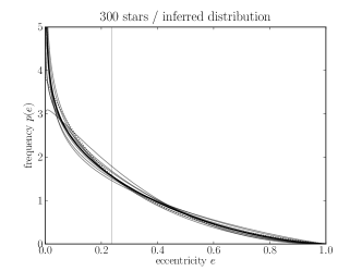
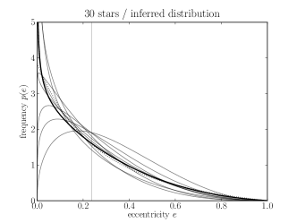
We repeat these experiments but now using the beta distribution for ${f_{\boldsymbol{\alpha}}}(e)$. Once again we perform Metropolis-Hastings MCMC, but now in the space of the beta-distribution shape parameters $\boldsymbol{\alpha}\equiv(a,b)$. Again the proposal distribution used in the MCMC was a small Gaussian perturbation applied to the two components of $\boldsymbol{\alpha}$, with Gaussian variance chosen to keep the acceptance ratio near 0.4. For each experiment $2\times 10^{3}$ links of MCMC were run, and checked for mixing. We show the results of the beta-distribution fitting in Figure 4. It also performs extremely well.

We obtained $K=10^{5}$ samples per star, but this is almost certainly overkill. In Figure 5 we show how the results change when this sampling is thinned down to just $K=50$ samples of the posterior PDF. The thinning was done uniformly, taking every 2000th sample from the parent set of $10^{5}$. The results are only slightly worse with $K=50$; this speeds up the code by a factor of 2000, of course.

Section 4 Discussion

We have shown that proper inference of the eccentricity distribution outperforms the naive approach of histogramming best-fit eccentricity values. Our inference proceeds by inserting the model eccentricity distribution as a prior on the eccentricities, after which a good eccentricity distribution is one that makes the data—the set of all exoplanet observations—probable. Because this method models the distribution prior to observation, it is effectively a deconvolution working on heteroscedastic data; it is a generalization to arbitrarily non-Gaussian uncertainties of previous work in this area (Bovy et al 2009b). There is nothing crucial about eccentricity; the method presented here can be applied to any problem in which the true distribution $f(x)$ is desired and there are only noisy measurements. As long as the measurements are presented as likelihood functions or samplings under an uninformative prior, the function $f(x)$ can be inferred as described here.

Though it is common for investigators to present as measured distribution functions the histogram of estimated values, sometimes even worse mistakes are made. For example, it is sometimes tempting for an investigator to see the output of the sampler as providing a better estimate of the distribution function. The thinking is “well, the object has some probability of being in each of these eccentricity bins, so I will add a bit into each bin on its behalf”. This thinking is wrong: It convolves the error-convolved distribution with the errors once again. We will not cite specific examples (to protect the guilty), but this is occasionally done and always incorrect.

One limitation of this study is that we made a simplifying assumption of a separable prior; that is, we imagined that there was one eccentricity distribution for all of the stars in the sample. In reality, the eccentricity distribution will depend on parent star and exoplanet parameters, and there will be no clean separation of the eccentricity distribution. There are two reactions to this. The first is to live with the result, understanding that the distribution returned by the method is correct for the specific sample in hand, marginalizing over all other parameters. The second is to permit non-separable distribution functions. In this latter case, hierarchical modeling becomes even more necessary. All of the correlations between orbital parameters or dependences on the parent star’s properties can be modeled on the prior level and fit as we did here. This situation is not substantially more complicated; it is just that the terms in the sum in the likelihood of equation (9) becomes a function of multiple parameters, and the parameterization of the function changes.

Another limitation of this work is that we only considered single-planet systems. This was in part because we do not have a simple prior for generating realistic multiple-planet systems, but also because there is nothing fundamental that changes if we switch to multiple-planet systems. We also permitted additional “jitter” in the observations but did not in fact add jitter or any other kind of additional noise or data outliers. Again, addition of these things—and proper modeling of them—changes the individual-object likelihood functions and samplings, but does not change the procedure by which the eccentricity distribution is inferred.

Finally, this study has some danger of “garbage in, garbage out:” we generated data in accord with our general expectations, and fit it in accord with those same expectations. This is a limitation of all studies on artificial data, of course. However, we note that the parameterized eccentricity distributions that we fit are mixtures of step functions and beta distributions; neither of these are related directly to—or even very appropriate for representing—either of the distributions we used to generate the ersatz data. Furthermore, the “uninformative” prior PDF we used in the exoplanet samplings were wrong, not just because it got the eccentricity prior PDF wrong (the subject of this Article) but because they also got the velocity amplitude $\kappa$ prior PDF wrong: The ersatz exoplanets were generated with isotropic inclinations and a power-law distribution of masses $m$; this does not generate a power-law frequency distribution in $\kappa$. That is, this method works well even when the priors in the other parameters are substantially wrong. And of course these prior PDFs can be inferred too, in a generalization.

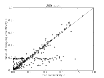
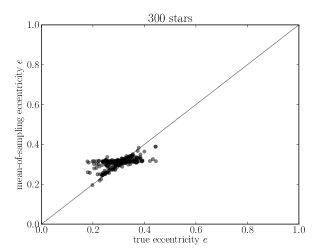
In Figure 2 and Figure 3, there are many objects whose eccentricities have been over-estimated by the maximum-likelihood method, some of them drastically. This arises naturally because the maximum-likelihood eccentricity tends to be higher than the true eccentricity, but it also arises a bit un-naturally because we have included in these figures some ersatz systems for which the exoplanet is not detected at significant signal-to-noise. That is, we threw in every system, even though at some periods, masses, and inclinations, the signal-to-noise is near or below unity. In most real experiments, these systems are removed (no-one measures the eccentricity distribution for undetected planets!). However, this method is not thrown off significantly by the low signal-to-noise systems. This is a good property of a proper probabilistic data analysis methodology: It is not moved around by the lowest signal-to-noise objects. Many popular methods in astrophysics do not have this simple property (necessary property, some would say). For example, in principal components analysis, the highest-noise systems often dominate the total data variance and therefore dominate the analysis. In general, measurements of variance (as measurements of distribution functions often are) can be thrown by noisy data. Forward models tend not to be.

In the real world, an investigator might want to infer the eccentricity distribution, but use input from many different exoplanet observers, each of whom might have sampled their exoplanets with different uninformative priors $p_{0}(e)$. This is not a problem; in the importance sampling of equation (9), the sum for each object $n$ should make use of the uninformative prior $p_{0}(e)$ used on object $n$. Also in the real world, an investigator might want to infer the eccentricity distribution using a mixture of measurements, some of which have been delivered as samplings, and some of which have been delivered just as maximum-likelihood estimates. Unfortunately these latter—maximum-likelihood estimates or any other single-point estimates—are nearly useless for modeling.

The method presented here is a baby step towards a hierarchical Bayesian method. The method would be fully hierarchical if we went back to the objects and re-sampled them using the inferred prior, or, even better, inferred the prior and performed the individual-object samplings simultaneously. That is, this method becomes fully hierarchical when the inferred distribution function is used to improve the individual-object estimates. When the measurements are given as likelihood functions, this should be the preferred method.

Along those lines, we could have performed a less simple but faster hierarchical sampling: Rather than marginalizing over the individual eccentricities by summing over a (potentially large) number of eccentricity samples for each exoplanet, we can use the provided samplings of the individual eccentricities as the basis of an approach that samples both the parameters of the eccentricity distribution and the true eccentricities of the planets. This approach avoids the sum in equation (9). It also returns updated posterior samples of the individual eccentricies using the better prior—the prior inferred from the population of planets.

Briefly, this approach entails writing down the joint posterior probability of the individual eccentricies and the parameters of the eccentricity distribution. Using Bayes’s theorem, we can write this joint distribution as

$$\displaystyle p(\{e_{n}\},\boldsymbol{\alpha}|\left\{{\boldsymbol{D}_{n}}\right\}_{n=1}^{N}) \propto p(\left\{{\boldsymbol{D}_{n}}\right\}_{n=1}^{N}|\{e_{n}\})\,p(\{e_{n}\}|\boldsymbol{\alpha})\,p(\boldsymbol{\alpha})\,.$$ (21)

By sampling from this posterior distribution, we simultaneously obtain samples of the eccentricities of the individual planets and of the parameters of the eccentricity distribution. These eccentricity samples will then have used the better eccentricity prior parameterized by $\boldsymbol{\alpha}$, rather than the uninformative original prior. For planets detected at low signal-to-noise, this leads to more realistic estimates of the eccentricity (see Figure 6).

We can re-write equation (21) as

$$\displaystyle p(\{e_{n}\},\boldsymbol{\alpha}|\left\{{\boldsymbol{D}_{n}}\right\}_{n=1}^{N}) \propto \left[p(\left\{{\boldsymbol{D}_{n}}\right\}_{n=1}^{N}|\{e_{n}\})\,p_{0}(\{e_{n}\})\right]\,\frac{p(\{e_{n}\}|\boldsymbol{\alpha})}{p_{0}(\{e_{n}\})}\,p(\boldsymbol{\alpha})\quad.$$ (22)

The provided eccentricity chains give us samples of the distribution in square brackets. We can re-use these samples in a manner similar to that in equation (9) to sample from the joint distribution of $\{e_{n}\}$ and $\boldsymbol{\alpha}$. Starting from initial $(\{e_{n}\}^{(i)},\boldsymbol{\alpha}^{(i)})$, first (1) Metropolis-sample $\{e_{n}\}^{(i+1)}$ from $p(\{e_{n}\}|\left\{{\boldsymbol{D}_{n}}\right\}_{n=1}^{N},\boldsymbol{\alpha}^{(i)})$ by sampling from

$$\displaystyle p(\left\{{\boldsymbol{D}_{n}}\right\}_{n=1}^{N}|\{e_{n}\})\,p_{0}(\{e_{n}\})\quad;$$ (23)

which can be done by just picking a random sample from the given eccentricity chains for the individual planets—and using the Metropolis-Hastings acceptance probability on

$$\displaystyle\frac{p(\{e_{n}\}^{(i+1)}|\boldsymbol{\alpha}^{(i)})\,p_{0}(\{e_{n}\}^{(i)}|\boldsymbol{\alpha}^{(i)})}{p(\{e_{n}\}^{(i)}\boldsymbol{\alpha}^{(i)})\,p_{0}(\{e_{n}\}^{(i+1)}|\boldsymbol{\alpha}^{(i)})}\quad.$$ (24)

Using this acceptance probability ensures that the samples are “importance-resampled” according to the new prior parameterized by $\boldsymbol{\alpha}$. Then, (2) sample $\boldsymbol{\alpha}^{(i+1)}$ from $p(\boldsymbol{\alpha}|\{e_{n}\}^{(i+1)})$ using any MCMC sampler. The resulting sampling of $\boldsymbol{\alpha}$ can then be used in exactly the same way as in Section 3.

Just to demonstrate the power of the hierarchical approach, in Figure 6 we show a comparison of the maximum-likelihood eccentricity estimates to the mean-of-sampling estimates made with the inferred prior. That is, we take the marginalized inferred distribution $\left<{f_{\boldsymbol{\alpha}}}(e)\right>$, re-weight the eccentricity samples with this inferred distribution, and produce as a point estimate for each system $n$ the mean of the re-weighted sampling. These mean-of-sampling estimates, made with a correctly informative prior, are—not surprisingly—better than the maximum-likelihood estimates.

In general, hierarchical inference must become a standard tool in astrophysics going forward: Our science is fundamentally statistical, and the objects of greatest interest are measured always at the limits of instrumental sensitivity. Hierarchical methods are the right tools for these jobs.

Figure 1: Two example ersatz exoplanets, one with relatively high signal-to-noise and one with relatively low. The top panels show the heteroscedastic radial velocity data with the true radial velocity model overplotted as a solid grey line, and the the maximum-likelihood (best-fit) radial velocity model overplotted as a dashed black line. The middle and bottom panels show the distribution of periods and eccentricities in ten percent of the $K=10^{5}$ samples in the thinned chain from the MCMC. Again, the solid grey line shows the true value, and the dashed black line shows the maximimum-likelihood value.

Figure 2: True, maximum-likelihood, and inferred eccentricity distributions for two samples of 300 ersatz exoplanets. The top panels show—as dotted curves—the frequency distributions from which the true eccentricities were drawn, the ST4 distribution on the left, and the Gaussian distribution on the right (see text for details). Superimposed is shown—as histograms—the obtained sampling of true eccentricities. The vertical lines indicate the means of the histogrammed distributions. The middle panels show—as histograms—the distributions of the maximum-likelihood (best-fit) eccentricities. Again, the vertical lines show the means of the histogrammed distributions. The bottom panels show a sampling—as a set of superimposed light histograms—of inferred distribution functions, drawn from the posterior PDF, and—as a solid line with dots—the marginalized inferred distribution (the mean of a $10^{4}$-point sampling). The vertical line shows the mean of the marginalized inferred distribution (the marginalized mean). The dotted curves are repeated in all panels to guide the eye.

Figure 3: Same as Figure 2 but for just the first 30 ersatz exoplanets.

Figure 4: On the left, similar to the bottom-left panel of Figure 2 (300 stars, ST4 distribution), but using the beta distribution rather than the step function for ${f_{\boldsymbol{\alpha}}}(e)$. The true ST4 distribution is shown with a dotted line, a sampling from the posterior PDF is shown with solid grey lines, and the marginalized inferred distribution (the mean of a $2\times 10^{3}$-point sampling) is shown with a solid black line. On the right, the same but similar to the bottom-left panel of Figure 3 (30 stars, ST4 distribution).

Figure 5: Same as the bottom row of Figure 2 but thinning the individual-exoplanet posterior PDF samplings down by a factor of 2000, from $K=10^{5}$ to $K=50$ samples per exoplanet.

Figure 6: Improving point estimates hierarchically. The top row shows a comparison of true eccentricities (for our ersatz exoplanets) with the maximum-likelihood estimates, for the ST4 (left) and Gaussian (right) true distributions. The bottom row shows the comparison of mean-of-sampling eccentricity estimates (see text), made using as prior PDFs on the eccentricity the (highly informative) marginalized inferred distributions of Figure 2. The horizontal line near 0.2 in the left figure and near 0.3 in the right figure comes from very low signal-to-noise systems (signal-to-noise at or below unity) for which the mean-of-sampling estimate ends up being very close to the mean of the prior PDF; this is the only reasonable mean estimate when the data are not informative.

References

- Balan & Lahav (2009) Balan, S. T. & Lahav, O., 2009, MNRAS, 394, 1936
- Blanton et al (2003) Blanton, M. R. et al, 2003, ApJ, 592, 819
- Bovy et al (2009a) Bovy, J., Hogg, D. W., & Roweis, S. T. 2009a, ApJ, 700, 1794
- Bovy et al (2009b) Bovy, J., Hogg, D. W., & Roweis, S. T. 2009b, arXiv:0905.2979
- Connolly et al (1995) Connolly, A. J., Csabai, I., Szalay, A. S., Koo, D. C., Kron, R. G., & Munn, J. A., 1995, AJ, 110, 2655
- Ford (2005) Ford, E. B., 2005, AJ, 129, 1706
- Gregory (2005) Gregory, P. C., 2005, ApJ, 631, 1198
- Hogg & Turner (1998) Hogg, D. W., & Turner, E. L., 1998, PASP, 110, 727
- Kitagawa & Gersch (1996) Kitagawa, G. & Gersch, W., 1996, Smoothness Priors Analysis of Time Series, Lecture Notes in Statistics 116 (Springer)
- Lehmann & Casella (1998) Lehmann, E. L. & Casella, G., 1998, Theory of Point Estimation (Springer)
- Loredo (2004) Loredo, T. J., 2004, American Institute of Physics Conference Series, 735, 195
- Lutz & Kelker (1973) Lutz, T. E., & Kelker, D. H., 1973, PASP, 85, 573
- Murray et al (2010a) Murray, I., Adams, R. P., & Mackay, D. J. C., 2010a, In Proceedings of the 13th International Conference on Artificial Intelligence and Statistics (AISTATS), Vol. 9, ed. Y. W. Teh & M. Titterington, 541
- Murray et al (2010b) Murray, I., & Adams, R. P., 2010b, arXiv:1006.0868
- Rasmussen & Williams (2006) Rasmussen, C. E. & Williams, C., 2006, Gaussian Processes for Machine Learning (MIT Press)
- Shen & Turner (2008) Shen, Y. & Turner, E. L., 2008 ApJ 685, 553
- Zakamska et al (2010) Zakamska, N. L., Pan, M., & Ford, E. B., 2010, MNRAS, in press (arXiv:1008.4152)