The JCMT Nearby Galaxies Legacy Survey V: The CO(J=3-2) Distribution and Molecular Outflow in NGC 4631

Abstract

We have made the first map of CO(J=3-2) emission covering the disk of the edge-on galaxy, NGC 4631, which is known for its spectacular gaseous halo. The strongest emission, which we model with a Gaussian ring, occurs within a radius of 5 kpc. Weaker disk emission is detected out to radii of 12 kpc, the most extensive molecular component yet seen in this galaxy. From comparisons with infrared data, we find that CO(J=3-2) emission more closely follows the hot dust component, rather than the cold dust, consistent with it being a good tracer of star formation. The first maps of $R_{3-2/1-0}$, H₂ mass surface density and SFE have been made for the inner 2.4 kpc radius region. Only 20% of the SF occurs in this region and excitation conditions are typical of galaxy disks, rather than of central starbursts. The SFE suggests long gas consumption timescales ($>$ $10^{9}$ yr).

The velocity field is dominated by a steeply rising rotation curve in the region of the central molecular ring followed by a flatter curve in the disk. A very steep gradient in the rotation curve is observed at the nucleus, providing the first evidence for a central concentration of mass: M${}_{dyn}\,=\,5\,\times\,10^{7}$ M_⊙ within a radius of 282 pc. The velocity field shows anomalous features indicating the presence of molecular outflows; one of them is associated with a previously observed CO(J=1-0) expanding shell. Consistent with these outflows is the presence of a thick ($z$ up to $1.4$ kpc) CO(J=3-2) disk. We suggest that the interaction between NGC 4631 and its companion(s) has agitated the disk and also initiated star formation which was likely higher in the past than it is now. These may be necessary conditions for seeing prominent halos.

1 Introduction

NGC 4631 (Fig. 1, Table 1) is an edge-on galaxy that is known for a spectacular multi-phase halo. This galaxy is one of the targets of the James Clerk Maxwell Telescope (JCMT) Nearby Galaxies Legacy Survey (NGLS) (Wilson et al., 2009; Warren et al., 2010) whose goals include searching for molecular gas and dust in nearby galaxies and comparing the global properties of such systems. In addition, the spatial and spectral coverage of the 325 - 375 GHz band presented by the new Heterodyne Array Receiver Programme - B-band (HARP-B) detector together with the wide-band Auto-Correlation Spectrometer Imaging System (ACSIS) has also made it possible to study individual galaxies in the sample in some detail. For NGC 4631, our goals are to examine the CO(J=3-2) properties and distribution in this unique galaxy and to relate, where possible, the molecular emission to known outflow features.

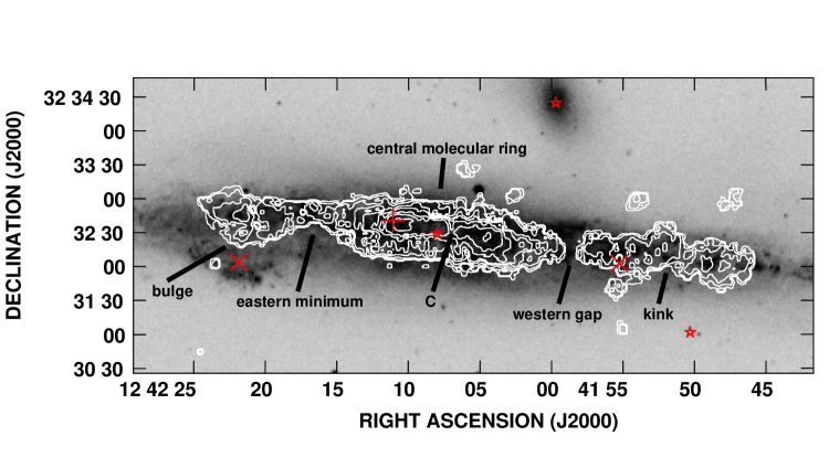
Figure 1: CO(J=3-2) integrated intensity (zeroth moment) map of NGC 4631 superimposed on the Second Digitized Sky Survey (DSS2) blue image. The CO(J=3-2) field of view shown here is 9.8^′ $\times$ 4.1^′ in right ascension and declination, respectively. Contours are at 0.25, 0.75, 2.0, 5.0, 8.0, 15, 24, and 45 K km s^-1 and the peak value is 57.7 K km s^-1. The moment-generating routine applied a spatial gaussian smoothing function of 40^′′ FWHM and a cutoff level of 0.018 K before integrating over the unsmoothed cube from 437 km s^-1 to 821 km s^-1 (see text). Red stars denote the centers of NGC 4631 (Table 1), the dwarf elliptical companion, NGC 4627 to the north-west, and the optical dwarf galaxy candidate, NGC 4631 Dw A, to the south-west. The red plus (+) and two crosses (X) denote the approximate centers of the CO(J=1-0) shell found by Rand (2000a) and the two HI supershells found by Rand & van der Hulst (1993, their Fig. 3), respectively. Features discussed in Sect. 3.1 are labelled.

The strength, prevalence, and multi-phase aspects of the halo of NGC 4631 make this galaxy unique and an important target for disk-halo studies. The halo is observed in all ISM components, including cosmic rays (CRs) and magnetic fields as indicated by polarized radio continuum emission (Golla & Hummel, 1994a; Hummel et al., 1991; Strickland et al., 2004a), HI (Rand, 1994; Rand & Stone, 1996) diffuse ionized gas (Martin & Kern, 2001; Rand et al., 1992; Otte et al., 2003; Hoopes et al., 1999), dust (Neininger & Dumke, 1999; Martin & Kern, 2001), molecular gas (Rand, 2000a), and hot, X-ray emitting gas (Vogler & Pietsch, 1996; Tüllmann et al., 2006a, b; Wang et al., 2001, 1995; Strickland et al., 2004a; Yamasaki et al., 2009). Expanding shells have also been observed in HI (Rand & van der Hulst, 1993) and CO(J=1-0) (Rand, 2000a). The halo extends over the entire star forming disk, reaching a variety of vertical heights, $z$, depending on the component considered, from 900 pc in molecular gas (Rand, 2000a) to 10 kpc in the radio continuum (Golla & Hummel, 1994a).

NGC 4631 is interacting with two companions, a dwarf elliptical, NGC 4627, $2.6^{\prime}$ (6.8 kpc, $\Delta V_{sys}\,=\,64$ km s^-1) to the north-west (Fig. 1) and NGC 4656, another large edge-on galaxy about $32^{\prime}$ (84 kpc, $\Delta V_{sys}\,=\,-40$ km s^-1) to the south-east, the result being 4 long intergalactic HI streamers (Weliachew, 1969; Weliachew et al., 1978; Rand, 1994) stretching to $\approx\,$42 kpc. The bases of these tidal streamers overlap with the halo of NGC 4631. In addition, three more faint companions have been detected in HI (Rand & Stone, 1996; Rand, 1994) as well as a faint optical dwarf galaxy candidate, NGC 4631 Dw A, $2.5$ kpc below the plane of NGC 4631 (Seth et al., 2005a) for which no redshift data are yet available. Of these companions, two (NGC 4627 and NGC 4631 Dw A) fall within the field shown in Fig. 1 and are marked with stars. Presumably, the star formation (SF) activity (and hence the halo) in NGC 4631 has been triggered and/or enhanced by interactions. Interactions have also likely produced the observed thick stellar disk, i.e. the optical emission shows $sech^{2}\left(z/z_{0}\right)$ scale heights, $z_{0}$, up to 1.4 kpc (depending on the stellar population considered) with detections to many scale heights in $z$ (Seth et al., 2005b).

Studies of the mid-IR emission and dust properties in NGC 4631 can be found in Draine et al. (2007), Dumke et al. (2004), Smith et al. (2007), Stevens et al. (2005), Bendo et al. (2003, 2006), and Dale et al. (2005, 2007). Previous CO observations in lower $J$ transitions have been carried out by Paglione et al. (2001), Golla & Wielebinski (1994b), Rand (2000a), Taylor & Wang (2003), and Israel (2009). Israel (2009) also obtained a CO(J=3-2) measurement in a single beam at the center of the galaxy. Limited previous CO(J=3-2) mapping has been carried out by Dumke et al. (2001) who detected emission only in the inner, 2.6^′ diameter region with a spatial resolution of $\approx\,23^{\prime\prime}$. The data presented here are of both higher resolution and sensitivity and, as will be shown, reveal the distribution of CO(J=3-2) both in the central regions as well as throughout the disk of NGC 4631.

Sect. 2 outlines the observations and data reductions. In Sect. 3 we describe the CO(J=3-2) distribution, and will be considering the distribution in the disk and a comparison with other wavebands, the CO(J=3-2) excitation, molecular mass and star formation, the velocity distribution and anomalous velocity and high latitude emission. Sect. 4 presents the discussion and Sect. 5 the conclusions.

Table 1: Basic Parameters of NGC 4631

parameter	value
Hubble type	SB(s)d sp or Sc sp
RA (J2000) (h m s)b	12 42 08.01
DEC (J2000) (∘ ′ ′′)	32 32 29.4
$V_{sys}$ (km s-1)	606
$D$ (Mpc)	9.0
a $\times$ b (′ $\times$ ′)	15.5 $\times$ 2.7
$PA$	86∘
$i$	86∘
$L_{FIR}$ (erg s-1)	$9.5\,\times\,10^{43}$
$L_{FIR}/D_{25}^{2}$ ($10^{40}$ erg s-1 kpc-2)	7.76
SFRFIR (M⊙ yr-1)	4.3
SFRHα,corr (M⊙ yr-1)	2.4
$M_{HI}$ (M⊙)	$1.0\,\times\,10^{10}$
$M_{dust}$ (M⊙)	$9.7\,\times\,10^{7}$

2 Observations and Data Reduction

Data were obtained of the ¹²CO(J=3-2) (rest frequency, $\nu_{0}$ = 345.7959899 GHz) spectral line at the JCMT using the HARP-B front-end and the ACSIS back-end (Smith et al. 2003). The HARP-B array contains 16 receivers in a 4 $\times$ 4 pattern separated by 30^′′ (about two beam-widths). In order to fully sample the field, the observing was set up as a sequence of raster scans in a “basket weave” pattern so that scanning was carried out in both the major and minor axis directions. The final sampling spacing was 1/2 of the beam size. Complete details of the observing set-up can be found in Warren et al. (2010) and Table 2. In total, 14 scans were obtained over two nights under good conditions with the $\nu\,=\,225$ GHz optical depth, $\tau_{225\,GHz}$, ranging from 0.051 to 0.070 on January 5 and from 0.041 to 0.068 on January 6. The calibration sources were IRC+10216 and Mars. Pointing offsets over the course of the observations were 2^′′ rms.

Data reduction was initially carried out using the Joint Astronomy Centre version of the Starlink software using the KAPPA, SMURF and CONVERT packages for editing, cube making, and converting to flexible image transport system (FITS) format, respectively. Visualization programs such as GAIA and SPLAT allowed us to inspect the data. Two of the 16 receptors were not functioning properly and had to be removed from all data. The editing was iterative, beginning by inspecting cubes from each scan individually, removing end channels, removing obvious interference spikes, binning to 20 km s^-1, removing a linear baseline, and then collapsing the cube to inspect the total intensity (zeroth moment) map. This usually revealed pixels that had obviously poor baselines for any given scan. Poor data points were removed from the unbinned, unbaselined data, and the process repeated, as required. All scans of the edited, but otherwise original resolution data were then combined into a single cube, using a ‘SincSinc’ kernel with a cell size of 3.638 arcsec (1/4 of the beam) and then saved in FITS format.

The fits cube was then read into the Astronomical Image Processing System (AIPS) package for the remainder of the processing and analysis. The data were box-car binned to a velocity resolution of 10.4 km s^-1 and a linear baseline was removed, fitted pixel by pixel. Some further minor editing was then carried out in AIPS. In addition, residual baseline curvature was still evident in some sections of the cube and these were then flattened using a 3rd order polynomial.

The final data were subsequently corrected for the main beam efficiency, $\eta_{MB}=0.60$ (estimated uncertainty between 10 and 15%) in order to convert into units of main beam brightness temperature, T_MB. Final channel maps for those channels that display emission are shown in Fig. 2a and b. The resulting measured rms noise (Table 2) per channel, met our goal for the NGLS. An examination of each individual HARP beam from independent observations of Mars shows that sidelobes of order 3% of the peak occur at distances of 24^′′ from the beam center which is well within our estimated uncertainties (see below). Sidelobes at larger distances are estimated to be less than this (P. Friberg, private communication) and therefore negligible.

A total intensity (zeroth moment) map was then made, which involved smoothing the data cube spatially, imposing a flux cutoff based on the smoothed cube, and then integrating in velocity over the original cube, using only those pixels that, in the smoothed cube, were above the flux cutoff. The result is shown in Fig. 1, with cutoff and smoothing details given in the caption. The field of view has also been reduced slightly (to 80% of the original) in order to trim noisy edge points.

The noise, taken to represent the uncertainty due to random errors in our total intensity map, is $\approx\,$1.6 K km s^-1, based on the noise per channel and number of channels entering into the sum at any typical position containing emission. In addition, we can compare our map to one obtained independently from the same data but using different software, editing, pixel size, channel width, and baseline smoothing (see Warren et al., 2010). The maxima of the two maps differ by 4%, and a histogram of the difference map is well fit by a Gaussian with a peak at 0.20 K km s^-1 and a standard deviation of 1.0 K km s^-1. These differences, the largest of which are likely due to differences in baseline flattening, are less than our estimated uncertainty above. Aside from these random errors, an absolute calibration error of 10 to 15% is present due to uncertainties in the value of $\eta_{MB}$; this uncertainty affects all pixels and does not change the appearance of the map. We have also compared the integrated intensity from the center of Fig. 1 to the single value given by Israel (2009) who also used the JCMT but with a different receiver. Our mean value of 24 $\pm$ 3 K km s^-1 in a 14.5^′′ beam agrees with his result of 22 $\pm$ 3 K km s^-1 in a 14^′′ beam at the same central position.

The ancillary data used in this paper were taken from the Spitzer Infrared Nearby Galaxies Survey (SINGS) Ancillary Data Archive unless otherwise indicated. The archive contains primarily Spitzer data but also includes ancillary images such as the H$\alpha$ image used in this paper. More information about the SINGS program can be found in Kennicutt et al. (2003).

Table 2: Observing & Map Parameters of NGC 4631

parameter	value
Observing Date	Jan. 05 & 06, 2008
Total bandwidth	1 GHz
Original channel width	0.488 MHz (0.43 km s-1)
Velocity-binned channel width	11.7 MHz (10.4 km s-1)
Angular resolution	14.5′′
rms (TMB) per channel	0.034 K

Figure 2: (a) CO(J=3-2) channel maps. Contours are at 0.10 ($3\,\sigma$), 0.20, 0.30, 0.50, and 0.75 K. The declination and right ascension scales are shown in Fig. 2b. The velocity of each channel is given at upper right and the beam is shown at the lower left of the first frame.

Figure 2: (b) CO(J=3-2) channel maps as in Fig. 2a.

3 Results

3.1 The CO(J=3-2) Distribution

As shown in the channel maps (Fig. 2) the east side of the galaxy is receding and the west side is approaching. Both the channel maps and the total intensity map (Fig. 1) show that the strongest emission is concentrated in a region of diameter, $3.8^{\prime}$ (10.0 kpc) centered on the nucleus (labelled the ‘central molecular ring’ in Fig. 1 for reasons outlined in the next subsection). At larger radii, there is weaker more extended disk emission. Several other features which we refer to below are also labelled in Fig. 1. Fig. 3 shows a slice in emission along the major axis of Fig. 1 at a position angle (83.5^∘) chosen so that it passes through the two broad maxima on either side of the nucleus (rather than the global optical major axis position angle of Table 1). Structures along the CO(J=3-2) major axis are well represented by this slice. In the next subsections, we discuss features associated with the disk of NGC 4631; discussion of the vertical distribution is deferred until Sect. 3.7.

3.1.1 The Strong Central Molecular Emission

The strong central molecular emission is characterized by two peaks on either side of the nucleus with a central minimum between them, and a slight major axis curvature that is well-known in this galaxy. This central emission extends between a minimum in the emission on the east (the ‘eastern minimum’) and a gap in the emission on the west (the ‘western gap’), as labelled in Fig. 1. The eastern peak is 15% higher than the western one, in agreement with the rudimentary CO(J=3-2) map of Dumke et al. (2001). Since the CO(J=1-0) distribution (Golla & Wielebinski, 1994b; Rand, 2000a) also shows a central minimum, the observed central CO(J=3-2) minimum cannot be a result of lack of sufficient excitation but must reflect a true minimum in the molecular gas distribution between the two peaks. A similar structure is also observed in dust emission (e.g. Bendo et al., 2002; Dumke et al., 2004; Bendo et al., 2006; Stevens et al., 2005); we discuss comparisons with other wavebands in Sect. 3.2.

Fig. 3 clearly shows that this double-peaked central molecular emission dominates the CO(J=3-2) distribution. The red curve represents an edge-on Gaussian ring with peak amplitudes that are slightly asymmetric and whose fitted parameters are given in Table 3. The emission was modelled following the method of Irwin (1994) and Irwin & Sofue (1996) which reproduces the line profiles of the cube. We imposed a cutoff radius at $100^{\prime\prime}$ in order to model the strong central emission only. The displayed model profile was then obtained in the same way as the data slice. This Gaussian ring describes the central emission very well except for excess emission in the wings at larger radii and also some departures near the nucleus. The inset shows the residuals.

The geometry of the central molecular gas distribution may be more complex than a simple ring. For example, bright spiral arms, rich in molecular gas of the kind seen in more face-on galaxies such as M 51 (Brunner et al., 2008), may mimic a ring or pseudo-ring when observed edge-on. There has also been some suggestion that NGC 4631 is barred. For example, there has been uncertainty in the optical classification (see Table 1) and Roy et al. (1991) have suggested that the entire region that we have modelled as a ring could be a large bar. A molecular bar could also mimic the distribution shown in Fig. 3, provided its density distribution is peaked at the bar ends. While this is possible, it has been shown (see Kuno et al., 2007, and references therein) that barred galaxies are much more likely to show strong central peaks or concentrations of CO, rather than the central minimum that we observe in NGC 4631. Rand (2000a) also finds no evidence for a bar, and a new high quality optical mosaic in gri colours from the Sloan Digital Sky Survey shows no clear bar in this galaxy either.

In summary, other specific geometries could be invoked to explain the strong central molecular emission, but since the Gaussian ring can do so with very few free parameters, we will use the term ‘central molecular ring’ to describe this region. Its velocity distribution will be discussed in Sect. 3.6.1 but it is worth noting here that the central molecular emission is kinematically distinct from the outer emission.

Table 3: Parameters of Modelled Central Molecular Ring

parameter	value
RA (J2000) (h m s)	12 42 7.7 $\pm$ 0.4
DEC (J2000) (∘ ′ ′′)a	32 32 30 $\pm$ 5
$i$ (deg)	89 $\pm$ 4
$R_{0}$ (′′, kpc)	42 $\pm$ 3, 1.8 $\pm$ 0.1
$D_{o}$ (′′, kpc)	6.4 $\pm$ 0.7, 0.28 $\pm$ 0.03
$D_{i}$ (′′, kpc)	2.1 $\pm$ 0.7, 0.09 $\pm$ 0.03

3.1.2 The Nucleus

As pointed out by Golla & Wielebinski (1994b), there are disagreements in the location of the center of the galaxy, depending on how the center is defined or which component is considered, consistent with a system that is highly disturbed. Fig. 1, for example, shows a central minimum in the CO(J=3-2) distribution (marked with a ‘C’). This minimum agrees with the minimum seen in the CO(J=1-0) map (Golla & Wielebinski, 1994b; Rand, 2000a) but is 15^′′ to the west of the infrared (IR) center of Table 1 (marked with a star).

The center of our modelled ring (Table 3), however, agrees with the IR center within uncertainties, but not with the position of C. The IR center coincides with the central radio peak (Golla, 1999), and our global CO(J=3-2) flux (not just the ring) is more symmetric about the infrared center than about C. In Sect. 3.6 we will also present a dynamical argument for the nucleus to be more closely represented by the IR center. Therefore in this paper, when we refer to the center or nucleus, we mean the IR center of Table 1. Note that there is a small peak in CO(J=3-2) right at the nucleus as can be seen in Fig. 3 (see also Sect. 3.6.1).

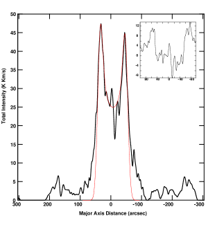
Figure 3: Slice along the major axis of the total intensity CO(J=3-2) distribution shown in Fig. 1, averaged over a width 11^′′ (3 pixels) in $z$. East is on the left and west is on the right. Offsets are with respect to the infrared center (Table 1). The thin red curve shows a gaussian ring with parameters as given in Table 3. The inset shows the residuals (data - model) for the central molecular ring.

3.1.3 The Weaker, Extended Disk Emission

In addition to the strong central molecular ring, we also observe weaker CO(J=3-2) emission at much larger radii, evidently associated with the larger rotating galactic disk (for example, see velocities of 499.3 km s^-1 and 738.3 km s^-1 in Fig. 2). This weaker broader disk emission appears distinct from the central molecular ring, separated from it by the eastern minimum and western gap (see Fig. 1); at these two locations, there is also an abrupt change in the rotation curve gradient (see Sect. 3.6). We will refer to this emission as the ‘outer disk’ to distinguish it from the central molecular ring.

This outer CO(J=3-2) disk tends to follow the optical disk emission. For example, the far eastern emission, centered at a right ascension of about 12^h 42^m 21^s (the ‘bump’, Fig. 1) maintains the bulging shape of the underlying optical disk. On the far western side there is a distinct corrugation in the CO(J=3-2) emission centered at a right ascension of $\approx$ 12^h 41^m 52^s (the ‘kink’, Fig. 1). The outer disk also harbours the two expanding HI supershells found by Rand & van der Hulst (1993) (marked with crosses in Fig. 1).

The maximum extent of the detected emission is 3.5^′ (9.25 kpc) to the east of the nucleus and 4.7^′ (12.4 kpc) to the west. This radial extent exceeds that of previous CO observations in any transition, although the CO(J=1-0) emission detected by Golla & Wielebinski (1994b) is almost as extensive to the west.

3.2 Comparison of Disk Emission with other Wavebands

The CO(J=3-2) emission is displayed in a number of overlays in Fig. 4 which show distributions that are taken to be proxies for unobscured star formation (H$\alpha$), the hot dust distribution (MIPS $\lambda\,$24 $\mu$m) and the cold dust distribution (MIPS $\lambda\,$160 $\mu$m). For the high resolution, high contrast $\lambda\,$24 $\mu$m map, we also show an inset of the central region. It is well known that molecular gas, dust and star formation correlate and we can see evidence for this in these overlays. For example, the CO(J=3-2) bump on the eastern side is evident in the H$\alpha$ map as well as the $\lambda\,$24 $\mu$m map, and the general trend of strong central emission and weaker secondary peaks at larger radii is common to the CO(J=3-2) and the two dust-emitting bands.

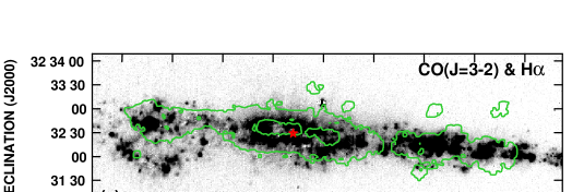
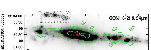
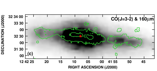
Figure 4: Overlays of the lowest and second highest contours of CO(J=3-2) emission from Fig. 1 on greyscales of (a) the H$\,\alpha$ image, (b) the MIPS 24 $\mu$m image, and (c) the MIPS 160 $\mu$m image. The greyscale images are shown at their original resolutions which are 3.0^′′ for the H$\,\alpha$ image (from measurements of point sources in the field), 6^′′ for the 24 $\mu$m image, and 40^′′ for the 160 $\mu$m image (Bendo et al., 2006). The greyscale ranges are arbitrary and have been chosen to emphasize low to moderate intensity features. For the high contrast, high resolution 24 $\mu$m image, we also show the central region in an inset. The star denotes the infrared center.

To explore these relations more quantitatively, Fig. 5 further shows comparative major axis slices of CO(J=3-2), $\lambda\,$24 $\mu$m, $\lambda\,$160 $\mu$m, and H$\alpha$ emission at a common spatial resolution and normalized to their peak flux values. Note that these slices contain most of the emission in any of the maps, since the width of the slice is 40 arcsec. Here, the general trend of the two dust components following the molecular gas distribution is again seen, but the departure of the H$\alpha$ emission is more obvious since this latter component is strongly affected by dust obscuration. The correlation coefficient is 0.99 between CO(J=3-2) and $\lambda\,$24 $\mu$m emission as well as between CO(J=3-2) and $\lambda\,$160 $\mu$m, whereas it is -0.001 between CO(J=3-2) and H$\alpha$ emission.

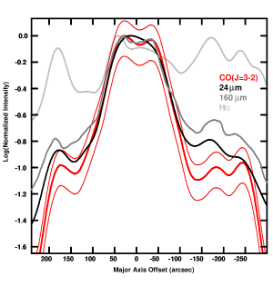
Figure 5: Comparison of major axis slices at 40^′′ resolution, averaged over 40^′′ in $z$ and normalized to their peak values. The positive x axis is to the east. The thick red curve shows the CO(J=3-2) emission taken from Fig. 1 and the thin red flanking curves show the extent of its error bars (which are the dominant uncertainties in the figure). The steep fall-off around +200 and -250 arcsec is due to the moment-generating routine. The black curve is the $\lambda\,24$ $\mu$m emission from Fig. 4b, the medium grey curve represents the $\lambda\,160$ $\mu$m emission from Fig. 4c and the light grey curve represents H$\alpha$ from Fig. 4a.

Focussing only on molecular gas and dust, Fig. 5 also shows that the CO(J=3-2) emission follows the hot dust emission ($\lambda\,$24 $\mu$m) more closely than the cold dust ($\lambda\,$160 $\mu$m). Colder dust displays a broader distribution that declines more slowly from the central molecular ring. Between $\pm$ 200 arcsec, for example, the mean of the ratios, CO(J=3-2)/$\lambda\,$24 $\mu$m and CO(J=3-2)/$\lambda\,$160 $\mu$m along the major axis (not shown) are 0.91 and 0.35, respectively, supporting the closer connection between CO(J=3-2) and hot dust. This result is consistent with the fact (see next section) that CO(J=3-2) is a good tracer of star formation and we would therefore expect it to be more closely aligned with hotter dust. Cold dust is more likely to trace both molecular gas farther from star forming regions as well as the more broadly distributed atomic component.

Bendo et al. (2006) have found that there is no significant variation with radius between the $\lambda\,70$ $\mu$m, $\lambda\,160$ $\mu$m, and $\lambda\,450$ $\mu$m emission in this galaxy and so we would expect plots of $\lambda\,70$ $\mu$m and $\lambda\,450$ $\mu$m emission to follow the cold dust emission of $\lambda\,160$ $\mu$m displayed in Fig. 5. Available $\lambda\,450$ $\mu$m data do not have sufficient signal-to-noise to test this but the close relation between $\lambda\,70$ $\mu$m and $\lambda\,160$ $\mu$m data allows us to repeat the above analysis at a higher spatial resolution (18^′′) using $\lambda\,70$ $\mu$m as a cold dust indicator. Again we find the same conclusion that CO(J=3-2) more closely follows hot rather than cold dust.

Fig. 5 appears to show an exception to this result right at the nucleus where there is a peak in the $\lambda\,24$ $\mu$m hot dust distribution but minima in both CO(J=3-2) and $\lambda\,160$ $\mu$m cold dust. However, at higher spatial resolution (see the inset of Fig. 4b) we see that the nuclear peak at $\lambda\,24$ $\mu$m is due to a strong ‘hot spot’ located within a region of approximately 17 arcsec (740 pc) diameter. As pointed out in Sect. 3.1.2, there is also a small CO(J=3-2) peak at the nucleus so the CO(J=3-2)/hot dust relation appears to hold even there, although relative emission strengths may vary. We will show in the next section that the star formation rate is higher at the nucleus than in the immediately surrounding region.

3.3 CO(J=3-2) Excitation

We can study the CO(J=3-2) excitation in NGC 4631 by forming a ratio map of CO(J=3-2) to CO(J=1-0) emission. To this end, we use CO(J=1-0) data obtained using the Berkeley Illinois Maryland Array (BIMA), originally at resolution of $\approx$ 8^′′, kindly supplied by R. J. Rand (Rand, 2000a). The total intensity CO(1-0) map from Rand (2000a) (his figure 1) was interpolated to the same grid as our total intensity CO(J=3-2) map and then both images were smoothed to 17^′′ resolution to reduce noise in the ratio map. The CO(J=1-0) map was then converted to units of K km s^-1. As a check on the CO(J=1-0) map, we made comparisons with previous single dish CO(J=1-0) data from the literature. As indicated by Rand (2000a), the BIMA total flux agrees with that of Golla & Wielebinski (1994b) within uncertainties. Also, the BIMA integrated intensity agrees with the Institut de Radioastronomie Millimétrique (IRAM) value at the same central position and resolution as given in Israel (2009). A comparison of major axis slices between the BIMA data and IRAM data of Golla & Wielebinski (1994b) at the same resolution also shows good agreement in the region of the central molecular ring. Both the BIMA map and our JCMT CO(3-2) map at 17^′′ resolution were then cut off at a conservative 5$\sigma$ level before forming the ratio. The resulting CO(J=3-2)/CO(J=1-0) map, $R_{3-2/1-0}$, shown in Fig. 6a, could be formed only over the brightest, inner 1.8^′ diameter (4.7 kpc) part of the central molecular ring, i.e. approximately over the FWHM of the emission shown in Fig. 3. The matching smoothed JCMT CO(J=3-2) map is shown in Fig. 6b.

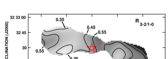
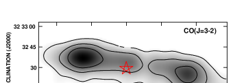
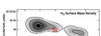
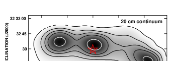
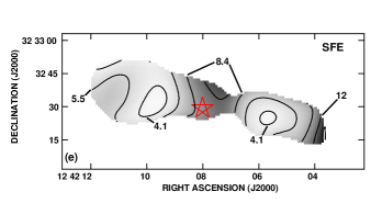
Figure 6: Comparison of emission in the brightest part of the central molecular ring. All maps have been smoothed to 17^′′ resolution, cut off at the 5$\sigma$ level, and are represented in both contours and greyscale with darker representing higher values. The star marks the galaxy’s center. (a) The integrated intensity ratio map, $R_{3-2/1-0}$. Contours are at 0.35, 0.45, 0.55, 0.65, and 0.75. (b) The JCMT CO(J=3-2) map in greyscale and contours of the inner region of Fig. 1. Contours are at 11, 22, and 33 K km s^-1 and the peak is 48.9 K km s^-1. (c) Molecular hydrogen surface mass density, $\Sigma_{H_{2}}$, formed from the CO(J=1-0) total intensity map, adopting X = $2.0\,\times\,10^{20}$ mol cm^-2 (K km s^-1)^-1. Contours are at 125, 200, and 350 M_⊙ pc^-2 and the peak is 380 M_⊙ pc^-2. (d) Radio continuum emission from the FIRST survey. Contours are at 3, 6, 9, 12 and 18 mJy beam^-1 and the peak is at 21.4 mJy beam^-1. The transformation to $\Sigma_{SFR}$ is given in Eqn. 2. (e) $SFE$, with contours at 4.1, 5.5, 8.4, and 12 $\times\,10^{-10}$ yr^-1. The peak is 17.3 $\times\,10^{-10}$ yr^-1.

To estimate the uncertainty in the $R_{3-2/1-0}$ map, we have formed a relative error map (not shown), based on random errors in the two individual maps. The average of the absolute values of the relative errors, is 11% (lower in regions of higher S/N). Errors due to positional offsets are much lower than this. Allowing for an additional absolute calibration error due to uncertainties in $\eta_{MB}$ (Sect. 2), we estimate that the average uncertainty in Fig. 6a is of order 25%. However, the calibration error can be neglected when examining the distribution of $R_{3-2/1-0}$ over the map since it would shift all points the same way. We have verified that our value of $R_{3-2/1-0}$ agrees with the result of Israel (2009) for the central position when smoothed to the same resolution.

The average value of $R_{3-2/1-0}$ over the region displayed in Fig. 6a is 0.47 with an rms of 0.11 and extrema of 0.24 and 0.92. Ninety-five percent of all pixels lie within the range, 0.28 to 0.66. These variations in $R_{3-2/1-0}$ appear to be real since they exceed the approximately 11% uncertainty discussed above.

Lower values of $R_{3-2/1-0}$, on average, are generally found for galaxy disks or for galaxies globally, for example those that are typically found in the molecular medium along the Milky Way disk ($\approx$ 0.4, Sanders, 1993), the disks of galaxies, or samples of nearby galaxies (0.2 to 0.7, Mauersberger, 1999; Wilson et al., 2009). Higher values, on the other hand, are seen in the central regions of galaxies (e.g. 0.7 to 1.2 for M 83, 0.9 for M 82, 0.6 for M 51, Muraoka et al., 2007; Tilanus et al., 1991; Israel et al., 2006, respectively), in high excitation regions or regions associated with star formation (e.g. up to 1.6 for the Antennae and up to 1.2 for specific regions in M 33, Petitpas et al., 2005; Tosaki et al., 2007, respectively), or in galaxies in which temperatures and/or molecular gas densities are higher, on average (Mauersberger, 1999). Therefore, the line ratios found in the central molecular ring of NGC 4631 appear to be typical of galaxy disks rather than of regions containing strong starbursts.

For the central 21 arcsec diameter region of NGC 4631 only, Israel (2009) finds that the molecular gas is best represented by two molecular components, with most of the mass (80%) in a cold ($T_{kin}\,=\,10$ K), tenuous (n${}_{H_{2}}\,\approx\,300$ cm^-3) component, and a lesser amount (20%) in a warm ($T_{kin}\,=\,150$ K), moderately dense (n${}_{H_{2}}\,\approx\,10^{3}$ cm^-3) state. Fig. 6a has now extended the measurement of $R_{3-2/1-0}$ over a much larger region than that measured by Israel (2009). With a single line ratio, we cannot place strong constraints on the state of the molecular gas over the extended region. In general, however, if a single physical state is present, the relationship between kinetic temperature, molecular gas density, and $R_{3-2/1-0}$ can be represented by Fig. 7 in which we show a large velocity gradient (LVG) model (e.g. Goldreich & Kwan, 1974; Irwin & Avery, 1992) with an abundance per unit velocity gradient of $X_{{}^{12}CO}/(dv/dR)\,=\,10^{-6}$ pc (km s${}^{-1})^{-1}$ (the latter value as suggested by the results of Zhu et al., 2003). Values of $R_{3-2/1-0}$ from 0.28 to 0.66 would then imply gas densities of order $10^{3}$ cm^-3 over the range of temperatures shown. Note that this density refers to the individual cloud densities that are responsible for CO excitation, rather than mean densities within the beam. If two components are present throughout the region with a lower density component dominating, such as found by Israel (2009) for the center, then $10^{3}$ cm^-3 should be an upper limit to $n_{H_{2}}$. Therefore, again we find that the conditions within molecular clouds in the central region of NGC 4631 appear to be typical of low density molecular gas regions in galaxy disks (i.e. $n_{H_{2}}\,<\,10^{4}$ cm^-3) rather than the $\,\hbox{\raise 2.15277pt\hbox{$>$}\kern-7.70004pt\lower 2.15277pt\hbox{$\sim$}$\,$}\,10^{4}$ cm^-3 which are more typical of central starburst regions (see, e.g. Weiß et al., 2001; Hailey-Dunsheath et al., 2008; Iono et al., 2007).

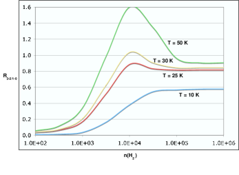
Figure 7: Plot of the ratio, $R_{3-2/1-0}$ as a function of molecular hydrogen density, $n_{H_{2}}$ (cm^-3) for a range of temperature (labelled) from an LVG code, assuming an abundance per unit velocity gradient of $X_{{}^{12}CO}/(dv/dR)\,=\,10^{-6}$ pc (km s${}^{-1})^{-1}$ and a single component model.

3.4 Molecular Mass and Gas/Dust Ratio

The distribution of molecular hydrogen mass surface density, $\Sigma_{H_{2}}$, in the central molecular ring of NGC 4631 is shown in Fig. 6c. This map was formed from the Rand (2000a) CO(J=1-0) map and therefore shows essentially the CO(J=1-0) distribution. We have used a standard and constant CO(J=1-0) integrated intensity to H₂ conversion factor of X = $2.0\,\times\,10^{20}$ mol cm^-2 (K km s^-1)^-1, consistent with Wilson et al. (2009), corresponding to 3.2 M_⊙ pc^-2 (K km s^-1)^-1 of molecular hydrogen (uncorrected for heavier elements). The mass distribution shows similar peaks and minima as the CO(J=3-2) map; differences are highlighted by the ratio map Fig. 6a. For this value of X the total molecular hydrogen mass over the region shown in Fig. 6c is M${}_{H_{2}}\,=\,7.4\,\times\,10^{8}$ M_⊙.

For this galaxy, there have been several measurements of the value of X from independent line ratio analyses. Israel (2009) finds X = $0.3\,\times\,10^{20}$ mol cm^-2 (K km s^-1)^-1 within the central 21 arcsec and Paglione et al. (2001) finds X = $0.5^{+2.0}_{-0.3}\,\times\,10^{20}$ mol cm^-2 (K km s^-1)^-1 within the central 46 arcsec and X = $1.8^{+7.1}_{-1.0}\,\times\,10^{20}$ mol cm^-2 (K km s^-1)^-1 outside of the central 46 arcsec. The two Paglione et al. (2001) values agree with each other and also with our adopted value within uncertainties. If we adopt the Israel (2009) value of X for the central 21 arcsec only, then M${}_{H_{2}}$ reduces by approximately 11% which is not significantly different from the above result, given the uncertainties. Although adopting a lower central value of X does not significantly perturb our calculation of total mass obtained from Fig. 6c, there would be changes in the appearance of this map, should X vary with position.

In addition, since we have observed CO(J=3-2) over a larger region than shown in Fig. 6, and to larger radii than previously detected in any CO transition, we can estimate the total molecular hydrogen mass in NGC 4631 by applying an appropriate value of $R_{3-2/1-0}$ over the entire emission shown in Fig. 1 and using the standard value of X listed above. Adopting the mean value from the central region, $R_{3-2/1-0}$ = 0.47, we find a total mass of M${}_{H_{2}}\,=\,2.2\,\times\,10^{9}$ M_⊙ with an error of $\approx$ 25% which represents the uncertainty in Fig. 6a including the calibration error. This uncertainty does not include uncertainties in X or in its possible variation with position in the galaxy. Our result has improved on that of M${}_{H_{2}}\,=\,1.5\,\times\,10^{9}$ M_⊙ (adjusted to our distance and value of X) provided by Golla & Hummel (1994a), whose map does not extend as far out as ours and who suggested a factor of 2 uncertainty on their quantity.

The total molecular gas mass is 22% of the total HI mass of M_HI = 1.0 $\times\,10^{10}$ M_⊙ found by Rand (1994) (Table 1). The total HI + H₂ mass is therefore M${}_{HI+H_{2}}\,=\,1.22\,\times\,10^{10}$ M_⊙ and dominated by HI. Adjusted for heavy elements (a factor of 1.36), the total gas mass is then M_g = $1.66\,\times\,10^{10}$ M_⊙ The total dust mass in NGC 4631 is estimated to be M${}_{d}\,=\,9.7\,\times\,10^{7}$ M_⊙ (Bendo et al., 2006), leading to a global gas-to-dust ratio of 170, a value that is typical of spiral galaxies, including the Milky Way (e.g. Draine et al., 2007). These masses are integrated over the entire galaxy and do not necessarily represent the relationships between atomic, molecular, and dust components in individual regions; we do not have sufficient information to determine region-specific quantities without a model for each of those components in this edge-on galaxy.

3.5 Star Formation

In Table 1, we list two estimates of the global SFR, the first from the FIR luminosity, and the second from the H$\,\alpha$ emission corrected for extinction using $\lambda\,24$ $\mu$m data (H$\,\alpha_{corr}$). The two values differ by about a factor of two. SFRs can be determined from a variety of different tracers but in a galaxy as edge-on as NGC 4631, optical depth effects can become large, uncertain, and can vary in an irregular fashion with position. The empirical relation for determining H$\,\alpha_{corr}$, for example, although considered relatively robust, has not been determined for galaxies that are edge-on (Calzetti et al., 2007). Fig 5 also confirms that there are large differences between the shape of the H$\,\alpha$ curve and other tracers that are not as badly affected by extinction. To probe the spatially resolved SFR, then, H$\,\alpha_{corr}$ cannot be used with full confidence (see also Footnote 37) and the FIR luminosity does not have sufficient resolution.

An alternative is to use radio continuum emission which requires no correction for optical depth effects and for which we have data for the high signal-to-noise region at the center of the galaxy as shown in Fig. 6d, taken from the Faint Images of the Radio Sky at Twenty-Centimeters (FIRST) survey (Becker et al., 1995) and smoothed from an original spatial resolution of 5 arcsec. The FIRST survey is insensitive to structure greater than 2^′ in scale which is approximately the diameter of the region shown in Fig. 6 and therefore there should be no missing flux on the scales that we are probing. In addition, although CR electrons diffuse from their source of origin in comparison to other tracers of SF, the scale over which this occurs for NGC 4631 (Marsh & Helou, 1998) is less than the beam size of Fig. 6. Finally, there is no evidence for a radio emitting AGN (or candidate) in this galaxy at a flux level that could affect the SFR determination (see Golla, 1999). The radio continuum is therefore a good measure of massive SF in the displayed region from which we can then estimate the total SFR.

We first use the relation given in Condon (1992) which provides only the massive ($M\,>\,5~{}M_{\odot}$) SFR, SFR_m from the radio emission, i.e.

$$\frac{{\rm SFR}_{m}}{[{\rm M}_{\odot}~{}{\rm yr}^{-1}]}\,=\,2.47\,\times\,10^{-22}\,\frac{L_{1.4}}{[{\rm W}~{}{\rm Hz}^{-1}]}$$ (1)

where $L_{1.4}$ is the 1.4 GHz radio luminosity per unit bandwidth and we have assumed that the 1.4 GHz emission is dominated by the non-thermal component with a typical spectral index of 0.8.

Integrated over the region displayed in Fig. 6d, we find SFR_m = 0.34 $M_{\odot}$ yr^-1 (or $\nu\,=\,0.014$ SNe yr^-1, from relations in Condon, 1992). We can also obtain SFR_m for the entire galaxy (not just the region shown in Fig. 6) from Eqn. 1 and the global radio continuum flux (771.7 mJy Strickland et al., 2004b) resulting in SFR_m = 1.8 ${\rm M}_{\odot}$ yr^-1. Therefore, $\approx\,$19% of the massive SF is occurring in the region shown in Fig. 6. Thus, the massive star formation in this galaxy is widely distributed in contrast to ‘nuclear starbursts’ such as M 82 (see also arguments in Tüllmann et al., 2006b). The Galaxy Evolution Explorer (GALEX) UV image also reveals widely distributed UV emission consistent with distributed star formation in this galaxy (de Paz et al., 2007).

We can now apply a factor to account for non-massive star formation, i.e. SFR/SFR${}_{m}\,=\,2.4$, where SFR is taken to be SFR_FIR from Table 1 and SFR_m is given above. Note that this correction factor is mid-range between the correction factors that would result by applying a disk IMF given by Chabrier (2003) (a factor of 1.1) and a Salpeter IMF (a factor of 5.5) over a total mass range of $0.1\,\leq\,{\rm M}\,\leq\,100\,{\rm M}_{\odot}$ yr^-1. The result, which converts the values of Fig. 6d to SFR per unit area, is

$$\frac{\Sigma_{SFR}}{[{\rm M}_{\odot}~{}{\rm yr}^{-1}\,{\rm pc}^{-2}]}\,=\,9.2\,\times\,10^{-6}\,\frac{I_{1.4}}{[{\rm Jy}~{}{\rm beam}^{-1}]}$$ (2)

We now provide a measure of the efficiency of star formation, $SFE$, in the central regions of NGC 4631 by forming the ratio map of ${\rm SFE}/[{\rm yr}^{-1}]\,=\,\Sigma_{\rm SFR}/[{\rm M}_{\odot}~{}{\rm yr}^{-1}~{}{\rm pc}^{-2}]/\Sigma_{H_{2}}/[{\rm M}_{\odot}~{}{\rm pc}^{-2}]$, which assumes that the stars mainly form in molecular gas (excluding HI). The result is shown in Fig. 6e. Note that we make no correction for inclination, so the values in this figure represent SFEs over the line of sight through the region. The mean value is ${\rm SFE}\,=\,6.4\,\times\,10^{-10}$ yr^-1 with an uncertainty of $2.5\,\times\,10^{-10}$ yr^-1 (based on the rms of the map) and extrema of $3.5$ and $17.3\,\times\,10^{-10}$ yr^-1. This result falls within the 1$\sigma$ error bar of the sample of Rownd & Young (1999) (after conversion to their definition of SFE) who examined global SFEs for 568 galaxies; that is, although there is a strong concentration of molecular gas in the central region of NGC 4631 and the galaxy is interacting (Sect. 1), the SFE in this region is typical of galaxy disks in general.

The inverse of SFE is a simple measure of the gas consumption timescale, $t_{g}$, if the SFR remains constant with time. Following Knapen & James (2009) and references therein, including a correction for recycling of material by stars into the ISM yields $t_{g}\,=\,1/(0.6\,{\rm SFE})$. For the region shown in Fig. 6e, we find a mean timescale of $\approx\,2.6\,\times\,10^{9}$ yr (to within approximately a factor of two, given the above uncertainties). This result will be a lower limit to the total gas consumption timescale since it does not include HI. From the arguments of the previous section, we expect the mean value of $t_{g}$ to increase by a factor of 2 or 3, should HI be included. All uncertainties considered, this result is still consistent with values found in other galaxies (Knapen & James, 2009; Bigiel et al., 2008; Leroy et al., 2008; Kennicutt et al., 1994; Golla & Wielebinski, 1994b). Clearly, the central region of NGC 4631 contains a strong build-up of molecular gas (Fig. 3), but the gas consumption timescale is long for a constant SFR. We return to this point in Sect. 4.

There is clearly a similarity between the $R_{3-2/1-0}$ map (Fig. 6a), representing molecular gas excitation (higher density and/or higher temperature as indicated by Fig. 7) and the SFE map (Fig. 6e) representing the star formation rate per unit molecular gas mass. Regions of lower ratio, as noted in Sect. 3.4 approximately correspond to regions of lower SFE – a trend also observed in M 83 by Muraoka et al. (2007). There are still differences, however. For example, a map of the ratio of SFE/$R_{3-2/1-0}$ (not shown) results in an rms variation of 25%, the most important difference being at the nucleus at which the SFE appears to be enhanced in comparison to $R_{3-2/1-0}$. Since both of these maps have been formed by normalization with the CO(J=1-0) distribution, the nuclear enhancement can be easily seen by directly comparing the CO(J=3-2) distribution of Fig. 6b (from which $R_{3-2/1-0}$ has been formed) to the 20 cm radio continuum map of Fig. 6d (from which SFE was derived). The radio continuum map shows a strong nuclear peak whereas the CO(3-2) map does not. Thus, there is an enhancement in SFR and SFE right at the nucleus in comparison to the surrounding region.

3.6 The Velocity Distribution

The global profile and position-velocity (PV) slices along and parallel to the major axis of NGC 4631 are shown in Fig. 8 and Fig. 9, respectively.

It is unusual to show a CO(J=3-2) global profile for a galaxy and Fig. 8 serves to illustrate the high quality of the HARP data. From this plot, the line width at half-maximum is $W_{50}\,=\,270\,\pm\,10$ km s^-1 and at 20% of maximum is $W_{20}\,=\,316\,\pm\,10$ km s^-1. From the mean midpoint of the linewidths, we find $V_{sys}\,=\,607\,\pm\,10$ km s^-1, in good agreement with the HI value of Table 1 as well as the HI value found by Rand (1994) (610 km s^-1) though it is somewhat lower than the CO(J=1-0) value of Golla & Wielebinski (1994b) (628 km s^-1) and Gao & Solomon (2004) (658 km s^-1). This global CO(J=3-2) value of $V_{sys}$ is plotted in Fig. 10a.

Figure 8: Global profile formed from the 3 central frames of Fig. 9. The rms is 0.5 K. The velocity is heliocentric.

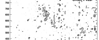
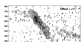
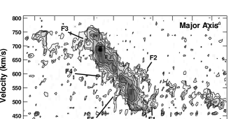
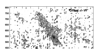
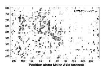
Figure 9: PV plots parallel to the major axis averaged over a width of 11^′′ (contours on greyscale). Vertical offsets (positive to the north) are marked on each frame. Contours are at 0.044 (2$\sigma$), 0.07, 0.10, 0.16, 0.25, 0.35, and 0.6 K. Positive is to the east on the x axis (50^′′ = 2.2 kpc). F1-F5 are discussed in Sect. 3.7.1.

The PV velocity distribution shown in Fig. 9 will be considered in three parts, namely, the central molecular ring and nucleus, the outer disk emission (both discussed below) and anomalous features and high latitude gas (to be discussed in Sect. 3.7).

3.6.1 The Central Molecular Ring and Nucleus

The most dominant emission shown in Fig. 9 is, again, the central molecular ring which extends 3.8^′ (10 kpc) in diameter (as noted in Sect. 3.1) forming a strongly emitting region with a steeply rising rotation curve. The velocity gradient is 2.1 km s^-1 arcsec^-1, or 48 km s^-1 kpc^-1 with an estimated 25% uncertainty depending on where the slope is measured. The fact that the western peak is stronger to the south (offset of -11^′′) and the eastern peak is stronger to the north (offset of +11^′′) reflects a slight asymmetry in the curvature of the major axis. (The major axis position angle of 6.5 deg was adopted to pass through both eastern and western maxima.) These gradients agree with those of the CO(J=1-0) distribution (Rand, 2000a).

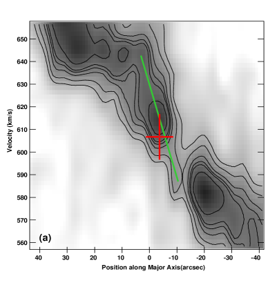
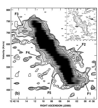
Figure 10: Enhanced versions of the major axis frame of Fig. 9. (a) Blow-up of the nuclear region emphasing the brightest emission with contours at 0.2, 0.25, 0.3, 0.33, 0.35 and 0.4 K. The x axis is centered on the IR center (Table 1). The cross marks the location of the modelled ring center in x (Table 3) and $V_{sys}$ (from the total global profile of Fig. 8), with the cross size delineating their respective error bars. The green line shows the nuclear gradient (see Sect. 3.6.1). (b) Here, the major axis has been smoothed spatially with a Gaussian of FWHM = 11^′′ to emphasize the fainter emission. Contours are at 0.028 ($2\,\sigma$), 0.035, 0.050 and 0.074 K. Features have been labelled as in Fig. 9. Inset: CO(J=1-0) major axis emission from the original data of Rand (2000a) rotated and smoothed as in the main figure; contours have been arbitrarily set.

An interesting new result is the ‘kink’ in the rotation curve approximately at the infrared nucleus of NGC 4631 such that in a single pixel (0.16 kpc) there is a vertical drop in velocity (east to west) of 25 km s^-1. Bright emission around the nucleus has been emphasized in the ‘blow-up’ of this region shown in Fig. 10a. The kink is seen at 640 km s^-1 just to the east (left in the figure) of the nucleus and the vertical drop continues to the west of the nucleus where the emission is much fainter since it falls within the emission gap denoted ‘C’ in Fig. 1. Similar behaviour can be seen in Offset $+11^{\prime\prime}$ frame of Fig. 9 and this steep gradient is also hinted at in the CO(J=1-0) data of Golla & Wielebinski (1994b). The nuclear gradient is delineated by the green line in the figure which has been adopted to pass through the small emission peak at the nucleus (this peak was pointed out in Sect. 3.1.2). Our modelled ring center (from Table 1) and our value of $V_{sys}$ (from the global profile of Fig. 8) are marked by the cross and agree, within uncertainties, with the center adopted for the nuclear gradient. This location appears to mark the galaxy’s true nucleus and is an additional argument (see also Sect. 3.1.2) for adopting the IR center as the location of the nucleus rather than the minimum at C.

The slope of the nuclear gradient is 4.1 km s^-1 arcsec^-1 (94 km s^-1 kpc^-1), much steeper than the rotation curve of the central molecular disk, implying the presence of a centrally concentrated mass of M${}_{dyn}\,=\,5\,\times\,10^{7}$ M_⊙ within a radius of 282 pc. To our knowledge, this is the first evidence for a concentration of mass at the center of NGC 4631.

3.6.2 The Outer Disk and Total Dynamical Mass

The weak outer disk emission becomes most evident at radii greater than 75^′′ (3.3 kpc) and appears kinematically distinct from the central molecular ring (see Fig. 9). Peak velocities at the largest measurable radii on either side of the nucleus are approximately the same as the peak values found in the central molecular ring, but in the region between the ends of the central molecular ring and the furthermost radii, velocities are lower, giving the impression that the rotation curve declines at the ends of the central molecular ring and then rises again with radius. However, a comparison with PV plots from the HI distribution shows that the rotation curve does not decline in this region (see Rand (1994), his Fig. 9); rather, it simply becomes flat at the ends of the central molecular ring and outwards. Therefore the appearance of lower rotational velocities just outside of the central molecular ring is a result of irregularities in the CO(J=3-2) emission intensity (see next section). Given the faintness of the CO(J=3-2) emission in the outer disk, it has not been possible to identify features corresponding to the HI supershells in these regions (Fig. 1).

Taking the mean of the maximum velocities ($V_{r}\,=\,155$ km s^-1) and radii ($R\,=\,10.6$ kpc) on either side of the nucleus and adopting a spherical distribution of total (light plus dark) mass for NGC 4631, the total mass is M${}_{tot}(R\,<\,11~{}{\rm kpc})\,=\,6\,\times\,10^{10}$ M_⊙. The HI distribution reaches comparable velocities (150 km s^-1) but can be detected to much larger radius, i.e. to $R\,\approx\,24$ kpc (Rand, 1994). From HI data, we can therefore extend the total mass estimate to $M_{tot}(R\,<\,24~{}{\rm kpc})\,=\,1.3\,\times\,10^{11}$ M_⊙.

3.7 Anomalous Velocity Features and High Latitude Molecular Gas

3.7.1 Anomalous Velocity Features

Fig. 9 reveals several anomalous velocity features which appear as extensions or partial loops in PV space associated with the central molecular ring. We have identified five such features (labelled F1 through F5 on the major axis slice) labelling only those that are connected to the central molecular ring and can be traced over at least two beam sizes spatially, at least two contiguous velocity channels, and over 2$\sigma$ in intensity. Two features, F1 and F3, occur near the ends of the central molecular ring and contribute to the (inaccurate) appearance of a declining rotation curve in these regions. To aid in visualizing these features, we have spatially smoothed the major axis slice of Fig. 9 and show the result in Fig. 10b with the same labelling. The inset shows the CO(J=1-0) data of Rand (2000a) treated similarly. Although the CO(J=1-0) data show significant noise, they do reveal some extensions at approximately the same locations of the features we have identified. We have also verified that these features exist in the CO(J=3-2) data cube that has been independently reduced by Warren et al. (2010) (see Sect. 2).

Some of the labelled features can be traced above or below the major axis. For example, the feature, F3, which appears loop-like on the major axis slice of Fig. 9, shows a split velocity profile above the major axis (Offset = +11^′′) open to the east. This feature corresponds to the expanding shell observed by Rand (2000a) in the CO(J=1-0) distribution. The feature, F2, shows complex structure (Fig. 10) but it can be traced south of the major axis (Offset = -11^′′ in Fig. 9) where it has the appearance of a smaller complete loop. The feature, F1, could be related to F2, though this association is not clear. Feature F4 appears to be an anomalous velocity extension to the main emission, and F5 forms a large, but weaker loop.

Since these features blend with the main emission in RA-DEC space, we cannot confirm shell-like structure spatially; however, the appearance of at least F2 and F3 in PV space are consistent with known behaviour of expanding shells or portions of expanding shells such as have been seen in our own and other galaxies in HI or CO (e.g. Spekkens et al., 2004; McClure-Griffiths et al., 2002; Irwin & Sofue, 1996; Lee et al., 2002; Weiß et al., 1999). F3 is the first detection in CO(J=3-2) of the previously known CO(J=1-0) shell and the other features are new detections.

In Table 4 we provide parameters of these features. The molecular masses may be lower limits because CO(J=3-2) emission represents only gas that shows some excitation and, in addition, we have determined the masses only over regions where the features clearly depart from the main disk emission in PV space. Nevertheless, we do find that our mass for F3 agrees with the value of $\approx\,10^{8}$ M_⊙ measured by Rand (2000a) for the corresponding CO(J=1-0) expanding shell.

The velocity width of these features, $\Delta\,V$, indicates that, even if no shell-like signature is observed, some expansion $V_{exp}\,=\,\Delta\,V/2$ must be occurring. From this information, we estimate the kinetic energy of the anomalous velocity features, $E_{K}$ (see Table 4). These energies may also be lower limits since they scale with mass. Although we are not certain of the origin of the features (see Sect. 4), it is common practice to estimate the input mechanical energies required to form them, $E_{0}$, assuming an instantaneous energy input, such as would be the case for clustered supernovae and stellar winds over a time scale that is short in comparison to the age of the feature itself. The required mechanical input energy is (Chevalier, 1974),

$$\frac{E_{0}}{\rm ergs}\,=\,5.3\,\times\,10^{43}\,\left(\frac{n_{0}}{{\rm cm}^{-3}}\right)^{1.12}\,\left(\frac{{R_{exp}}}{\rm pc}\right)^{3.12}\left(\frac{V_{exp}}{{\rm km~{}s}^{-1}}\right)^{1.4}$$ (3)

where $n_{0}$ is the ambient density at the time of the energy deposition and $R_{exp}\,=\,D/2$ is the shell radius. If a continuous energy input is assumed instead, the results tend to be consistent with Eqn. 3 to within a factor of a few (see Spekkens et al., 2004). Models such as these typically assume a uniform ambient density in the plane which is certainly not the case for molecular clouds. For NGC 4631, most of the molecular mass is in clouds with densities $\approx$ 300 cm^-3 (see Sect. 3.3). Since we estimate that there are roughly equal HI and H₂ masses in the region of the central molecular ring (Sect. 3.4) and the model of Rand (1994) estimates the ambient HI density in the plane to be $0.4$ cm^-3, then the average H₂ density could be similar, leading to a volume filling factor of $\approx\,10^{-3}$ for the molecular clouds. Although these are very rough estimates, most of the molecular outflow would be through in-plane densities that are lower than those of the molecular clouds themselves. We have therefore used $n_{0}\,=\,0.4$ cm^-3 in Eqn. 3, bearing in mind that the results for $E_{0}$ will be conservative estimates since higher densities could be important at some level.

Finally, we compute ‘characteristic’ ages, $\tau$, which do not take into account accelerations or decelerations over the development of the feature. If a continuous wind model is adopted, these lifetimes would decrease by approximately a factor of three (McClure-Griffiths et al., 2002). It is interesting that all lifetimes fall into a narrow range of timescales, $\tau\,\approx\,2\rightarrow 2.6\,\times\,10^{7}$ yr, suggesting that they may be related to a single burst of star formation. Note, however, that our spatial resolution selects features that are of kpc scale and these observations would not have detected smaller, and therefore younger, features, if they were present. Larger features may also be difficult to detect if their densities diminish with increasing size.

The CO(J=3-2) shell results of Table 4 are similar to those of HI shells found in our own Milky Way and external galaxies (e.g. Brinks & Bajaja, 1986; Puche et al., 1992; McClure-Griffiths et al., 2002; Chaves & Irwin, 2001; Spekkens et al., 2004, and others). The tabulated masses and energies, although order of magnitude estimates, are likely conservative as discussed above; it is clear that many hot young stars and supernovae would be required to form the features if they are indeed the origin. We will return to this issue in Sect. 4.

Table 4: Parameters of the Anomalous Velocity Features

Feature	RA0 a, DEC0 a	$V_{0}$	$D$	$\Delta\,V$	Mmol	$E_{K}$	$E_{0}$	$\tau$
	(h m s, ∘ ′ ′′)	(km s-1)	(′′, kpc)	(km s-1)	(107 M⊙)	($10^{53}$ ergs)	($10^{53}$ ergs)	($10^{7}$ yr)
F1	12 42 00, 32 32 15	500	22, 0.95	52	2.3	1.6	4.1	1.8
F2	12 42 03, 32 32 13	593	44, 1.9	73	5.3	7.1	57	2.5
F3	12 42 14, 32 32 40	718	33, 1.4	62	9.0	8.6	18	2.2
F4	12 42 10, 32 32 29	593	22, 0.95	42	3.0	1.3	3.0	2.2
F5	12 42 07, 32 32 25	468	44, 1.9	73	2.4	3.2	57	2.5

3.7.2 High Latitude Molecular Gas

As indicated in the previous section, the anomalous velocity features seen in the PV plots (Fig. 9) are not easily traced to high latitudes. However, we do see some evidence for the presence of high latitude CO(J=3-2) in the data.

Fig. 1 shows that the disk thickness of NGC 4631 varies with position, but at least within the central molecular ring, the evidence suggests that NGC 4631 forms a thick, rather than a thin distribution. A thin global molecular gas disk with the observed diameter of the CO(J=3-2) emission (see Sect. 3.6.2) which is inclined by 86^∘ (Table 1) would project to a total apparent vertical extent of only 48^′′ including the smoothing effects of the beam, whereas the total observed minor axis extent is approximately 65^′′ (2.3 kpc after beam correction, or $z\,=\,1.2$ kpc). If the inclination of the central molecular ring were as low as 83^∘, then it could be interpreted as thin. However, our model of the central molecular ring (Table 3) gives best results for an even higher inclination ($i\,=\,89^{\circ}$); lower values are poorer.

To further investigate the vertical extent of the molecular gas, we have formed a plot at high sensitivity showing the minor axis profile by averaging over a 100^′′-wide region of the major axis (i.e. approximately over the FWHM of the central molecular ring) and then averaging the north/south sides. The result, shown in Fig. 11, reveals a complex profile which is not well described by a single smooth fit. CO(J=3-2) can be traced out to $z\,=\,33^{\prime\prime}$ (1.4 kpc), correcting for beam smoothing. Thus, the central molecular ring of NGC 4631 appears to have a thick vertical distribution of CO. Given the known halo activity in this galaxy, most of which has been measured to much larger values of $z$ (see Sect. 1), the presence of thick, agitated molecular gas is perhaps not surprising. For comparison, we note that main sequence stars in NGC 4631 have been measured out to a $z$ height of 2.3 kpc and AGB and RGB stars have been measured to even higher $z$ values (Seth et al., 2005b).

Figure 11: Vertical profile of the CO(J=3-2) emission of NGC 4631, formed from Fig. 1 averaged over a 100^′′ wide region centered at the nucleus. The profiles to the north and south have also been averaged to form a sensitive plot. The emission cuts off at $z\,\approx\,40^{\prime\prime}$ due to the algorithm for determining the total intensity image (see caption of Fig. 1). The projected minor axis extent of a thin disk of radius, $R\,=\,243^{\prime\prime}$, inclined at $i\,=\,86^{\circ}$ ($R\,cos(i)$) and then smoothed by the beam, is given by the thick vertical line segment.

We see no evidence from the PV plots (Fig. 9), however, for a change in the slope with $z$ height (‘lagging halos’) such as has been seen in HI or ionized extraplanar gas in several other galaxies (e.g. Tüllmann et al., 2000; Rand, 2000b; Fraternali et al., 2002; Oosterloo et al., 2007) although the vertical extent of molecular gas in NGC 4631 is, in general, smaller than these other components.

Fig. 1 also shows a number of disconnected emission features above and below the plane at distances of $50^{\prime\prime}\,-\,60^{\prime\prime}$ ($z\,\approx\,2.2\,\rightarrow\,2.7$ kpc). The smoothing and noise cut-off techniques used to create the total intensity image are ideal for emphasizing such low level emission which generally can only be seen in cubes that are smoothed, rather than in the original channel maps. Their emission is contiguous in velocity space and several can be identified in the independently reduced, lower velocity resolution data of Warren et al. (2010). However, since not every one can be independently confirmed, we do not label each individually and only consider the energetics (below) of a ‘typical’ feature. For the purpose of discussion, we refer to them as high latitude ‘clouds’.

Fig. 12, which emphasizes the low level emission of Fig. 1, shows how these clouds exist above apparent disturbances in the disk. For example, there are clouds both above and below the location of the western HI supershell (the western X). There is also a cloud above the plane and a complete loop below the plane at the location of feature F5. These clouds have masses of M${}_{cl}\approx\,10^{6}$ M_⊙ and estimated potential energies of,

$$\frac{\Phi(z)}{\rm ergs}\,=\,2\,\times\,10^{54}\,\left(\frac{{\rm M}_{cl}}{2\,\times\,10^{7}~{}{\rm M}_{\odot}}\right)\,\left(\frac{z_{0}}{700~{}{\rm pc}}\right)^{2}\,$$

$$\cdot\left(\frac{\rho_{0}}{0.185\,{\rm M}_{\odot}~{}{\rm pc}^{-3}}\right)\times\,ln\left[cosh\left(\frac{z}{z_{0}}\right)\right]$$ (4)

(e.g. Spekkens et al., 2004), where $z_{0}$ is the mass scale height and $\rho_{0}$ is the mid-plane mass density with the normalization factor taken to be an estimate for the local Solar neighbourhood. Adopting the stellar scale height of $z_{0}\,=\,1$ kpc from Seth et al. (2005b) we find,

$$\frac{\Phi}{\rm ergs}\,\approx\,3.7\,\times\,10^{53}\,\left(\frac{\rho_{0}}{0.185\,{\rm M}_{\odot}~{}{\rm pc}^{-3}}\right)$$ (5)

which suggests that kinetic energies of this order are required to place the molecular clouds at their observed heights. Input energies are likely higher still (cf. $E_{K}$, $E_{0}$ in Table 4) if these clouds have originated in the disk. Further discussion can be found in Sect. 4.

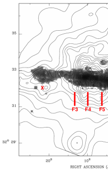
Figure 12: CO(J=3-2) map of Fig. 1 with low level emission emphasized overlaid with X-ray contours representing hot gas (from the data of Wang et al. 2001). Approximate locations of the features identified in Fig. 9 are marked as well as the two HI shells (marked with X) identified by Rand & van der Hulst (1993).

3.7.3 Comparison of Outflow and High Latitude Features with other Wavebands

As indicated in Sect. 1, the halo of NGC 4631 has been observed in every ISM component. Since the halo is so extensive and there is overlap with the broader HI tidal streamers, some caution must also be exercised in identifying correlations as they may be due to chance projections along the line of sight (see e.g. Taylor & Wang, 2003). The features that we have identified (Table 4) are mostly visible in PV space, rather than in RA-DEC and we have thus not found counterparts at other wavebands, other than F3 as noted in Sect. 3.7.1 which is associated with a CO(J=1-0) expanding shell.

A possible high latitude dust arch, discovered by Neininger & Dumke (1999), but interpreted as part of HI tidal spur 4 by Taylor & Wang (2003), has its footprint in the disk at approximately the position of the west HI expanding shell. At this location, early X-ray images show hot gas extending into the halo, as shown most clearly in Wang et al. (1995) (their Fig. 1a). More recent X-ray images (see Fig. 12) show emission from hot gas which has originated from the disk and is associated with H$\alpha$ emission and a ‘froth’ of superbubbles (Wang et al., 2001). Given the varying distributions of the X-ray and CO(J=3-2) components and the edge-on nature of the galaxy, Fig. 12 does not show clear correlations between the two components. However, it is clear that the stronger X-ray halo emission is located over the region of the central molecular ring.

Finally, one high latitude CO(J=3-2) feature, namely the southern loop associated with F5 (Fig. 12), does appear to have an H$\alpha$ counterpart in the form of two H$\alpha$ spurs, the latter seen in Fig. 4a. To the east of the two spurs is a third H$\alpha$ spur that appears to have a counterpart in the $\lambda\,160$ $\mu$m emission (Fig. 4c).

4 Discussion

A picture has emerged of NGC 4631 as an actively star forming galaxy, but not one with a central starburst. Approximately 80% of the massive star formation in this galaxy occurs outside of the central 1.8^′ (4.7 kpc) diameter region and H$\alpha$ and UV emission in the disk are also widely distributed. The X-ray halo (Fig. 12), which resembles the well-known radio halo (Wang et al., 2001), is similarly widespread over the entire star forming disk. Widespread halo emission is seen in all ISM components (see Sect. 1 for references) and all evidence, including the presence of HI supershells, a CO(J=1-0) expanding shell, vertical filaments, the vertical structure of the magnetic field lines, the concentration of stronger halo emission over stronger star forming regions in the disk, and now CO(J=3-2) anomalous velocity features point to star forming regions and their related supernovae and stellar winds in the disk as the origin of the halo. The question is, why does NGC 4631, whose halo is arguably the most spectacular ever observed, have such a wide-spread, prominent halo in comparison to other edge-on galaxies?

To consider this question, it is worth comparing NGC 4631 to two other galaxies: NGC 5775, which has a similarly wide-spread multi-phase halo (Lee et al., 2001; Li et al., 2008), and M 82, which is the prototypical nuclear starburst with bipolar outflow. All three galaxies have significant companions with which they are interacting, the most obvious evidence being the presence of HI bridges or streamers between them (Yun, Ho, & Lo, 1994; Irwin, 1994; Weliachew et al., 1978). For NGC 4631, the interaction is with the large spiral, NGC 4656 and the dwarf elliptical, NGC 4627 (Sect. 1). These interactions may have played an important role in forming their halos via tidal disruptions or agitation of the disk. For example, if the disk has become ‘puffed up’, such as we seem to see in the thick CO(J=3-2) layer in NGC 4631 (Sect. 3.7.2), it would be easier for material to escape into the halo. Stellar winds and supernovae should also produce thickened gaseous disks as material escapes vertically into the halo. For NGC 4631, since the stellar disk also extends several kpc above the plane (Sects. 1, 3.7.2), the interaction has most likely played an important direct role.

As for star formation, M 82, NGC 5775 and NGC 4631 all have similar FIR luminosities to within a factor of about 2, but their luminosities per unit optical disk area, a distance-independent quantity, vary in the ratio, 1:0.16:0.05 in the order listed above (Tüllmann et al., 2006a). NGC 5775 and NGC 4631, which both show disk-wide halos, differ by only a factor of 3. M 82, on the other hand, has a SFR per unit area that is higher than that of NGC 4631 by a factor of 20. Since M 82 has been well-studied, it is possible to compare activity within the nuclear region itself. For M 82, the supernova rate in the central 700 pc is $\nu\,=\,0.1$ yr^-1 (Kronberg et al., 1981). From Eqn. 1, Fig. 6d, and relations in Condon (1992), we find $\nu\,=\,0.001$ yr^-1 for an equivalently sized region at the center of NGC 4631. That is, the central supernova rate in NGC 4631 is two orders of magnitude smaller than in M 82, hence the nuclear outflow in M 82 but not in NGC 4631.

It is well known that interactions can trigger a build-up of molecular gas in galaxy centers and can also induce strong central starbursts (e.g. Aalto, 2007). What is particularly striking about NGC 4631 is the presence of strong central molecular emission in a ring out to a radius of $\approx$ 5 kpc (e.g. Fig. 3) but without a central starburst. The physical properties of the ring are typical of galaxy disks, rather than other known nuclear starbursts (Sect. 3.3) and the star formation efficiency is not very high; that is, if SF continues at the current rate, there is sufficient molecular gas to sustain it for at least $3\,\times\,10^{9}$ yr. Inside the ring, within the central 17^′′ (740 pc) diameter region (Fig. 6) the SFR is enhanced and there is a peak in the hot dust distribution (Fig. 5) as well as a small peak in CO(J=3-2) (Fig. 3). Even here, however, the gas consumption time scale is at least $10^{9}$ yr. If the interaction is to trigger a central starburst in NGC 4631, then it has already happened or it has not happened yet.

Knapen & James (2009) have added further confirmation to the notion that, although bursts of SF can occur as a result of interactions and there is a tendency for the star formation to be centrally concentrated, interactions can also initiate continuous star formation over longer timescales, ie. a few $\times\,10^{8}$ yrs (see also Di Matteo et al., 2008). For NGC 4631, the interaction with its companion occurred $\approx\,3\,\times\,10^{8}$ years ago (Combes, 1978). There is some evidence that at least one burst of star formation (or higher SFR) has already occurred in NGC 4631. From UV observations Smith et al. (2001) note that the current rate of SF does not seem to account for other indications of strong outflow in this galaxy. For example, the eastern HI shell (see Fig. 1) can be explained by supernovae from a massive SF region containing $5.3\,\times\,10^{4}$ OB stars beginning about $2\,\times\,10^{7}$ yr ago and that the currently observed UV emission (which is insufficient to explain the shell) is due to second generation stars. Our own estimates for the lifetimes of the observed CO(J=3-2) anomalous velocity features are approximately the same (Table 4) and, estimated the same way, the HI supershells observed by Rand & van der Hulst (1993) also result in ages of a few $10^{7}$ yr. These results suggest that a higher rate of SF may have occurred of order $\approx\,10^{7}$ yr ago. However, as noted in Sect. 3.7.1, selection effects may have prevented us from detecting features with larger or smaller lifetimes, so we cannot place a limit on the timescale for past SF in general.

Estimates for the kinetic energies of the anomalous velocity features are of order $E_{K}\,\approx\,10^{53}$ ergs and estimates of potential energy of the small clouds above and below the plane are about the same (Sect. 3.7.2). The implied input energies are higher still, possibly by an order of magnitude (Table 4), a conclusion also implied for the energetics of the outflowing molecular gas in the nuclear outflow of M 82 (Seaquist & Clark, 2001). These energies are also typical of what has been previously seen for HI and CO expanding shells in other galaxies (Sect. 3.7.1) and are quite high. If the observed features are associated with a higher SFR in the past as suggested above, however, the energies may be sufficient. Supernovae from the stars that are believed to be responsible for the eastern HI supershell could supply (at 10⁵¹ ergs each) $5.3\,\times\,10^{55}$ ergs for this shell which is more than adequate. However, there would need to be at least five such SF regions throughout the region of the central molecular ring to account for all of the features of Table 4. There is still some need for time-dependent modelling of such outflows in a realistic multi-phase, multi-density, and magnetised ISM.

The prominent radio halo in NGC 4631 actually reflects an integration over past SF activity in the disk. The average magnetic field strength in the disk of NGC 4631 is $B\,=\,6.5$ $\mu$G (Dahlem, Lisenfeld & Golla, 1995) with a CR electron lifetime estimate of $t_{CR}\,=\,4.8\,\times\,10^{7}$ yrs. The ratio between the halo and disk magnetic field strength is 5/8 (Hummel et al., 1991) yielding an average halo field strength of $B\,=\,4$ $\mu$G and, since $t_{CR}\,\propto\,B^{-3/2}$, the CR lifetime in the halo is $t_{CR}\,\approx\,10^{8}$ yrs. Consequently, the radio halo that we see today has a memory of outflows that have occurred since approximately the time that the interaction occurred, assuming that the outflows have not escaped into the intergalactic medium. Whether or not this assumption is correct requires deeper and more extensive mapping of the magnetic field direction than is currently available. However, arguments presented in Seaquist & Clark (2001) suggest that even in the more energetic nuclear outflow of M 82, at least the molecular gas and dust do not escape.

The implication of a higher SFR in the past suggests that, when strong halos such as in NGC 4631 and NGC 5775 are observed, they may have been enhanced by a previous outflow event (or events). Although rather speculative, another possibility is that such galaxies have also experienced a stronger M 82-like starburst and nuclear outflow in the past that was triggered by the interaction. In the case of NGC 4631, the enhanced SFR right at the nucleus could be a remnant of a past ‘M 82-like’ nuclear starburst. We could imagine the interior of the nuclear molecular ring to have been excavated by massive star formation and outflow. The minimum near the nucleus at ‘C’ (Fig. 1) could reflect local variations in SFR and molecular content. The past additional ‘boost’ of outflow material into the halo may be what is required to distinguish between spectacular halos and those that are more modest.

5 Conclusions

As part of the JCMT Nearby Galaxies Legacy Survey, we have mapped the CO(J=3-2) emission from the edge-on galaxy, NGC 4631, which is known for its spectacular multi-phase gaseous halo.

Most of the CO(J=3-2) emission is concentrated within a radius of $\approx$ 5 kpc. Although the spatial distribution could be more complex, the emission is well modelled by a simple edge-on ring with a Gaussian density distribution which peaks at a radius of 1.8 kpc and has inner and outer scale lengths of 0.1 and 0.28 kpc, respectively. The center of the ring agrees with the IR center. A small CO(J=3-2) peak occurs within this ring, right at the nucleus. Outside of the central molecular ring, weaker more extensive disk emission is present which has been mapped out as far as 9.25 kpc to the east of the nucleus and 12.4 kpc to west. This radial extent exceeds that of any previous CO observations.

Comparisons have been made between CO(J=3-2), $\lambda\,24~{}\mu$m, $\lambda\,160~{}\mu$m emission and H$\,\alpha$. We find that the CO(J=3-2) emission more closely follows $\lambda\,24~{}\mu$m (a hot dust tracer) rather than $\lambda\,160~{}\mu$m emission (a cold dust tracer), suggesting that CO(J=3-2) is a good tracer of star formation. H$\,\alpha$ emission is uncorrelated because of the high extinction in this edge-on galaxy.

For the inner 2.4 kpc radius region of the central molecular ring, we have formed the first spatially resolved maps of $R_{3-2/1-0}$, the H₂ mass surface density, and the SFE for NGC 4631. Only 20% of the global SF occurs in this region. We find that $R_{3-2/1-0}$ is typical of galaxy disks, in general, rather than of regions associated with central starbursts. Molecular cloud densities ($\approx\,10^{3}$ cm^-3) in this region are also typical of molecular clouds in galaxy disks rather than central starbursts. The SFE in this region is, on average, $6.4\,\times\,10^{-10}$ yr^-1 leading to a mean gas consumption timescale of $2.6\,\times\,10^{9}$ yr for the H₂ and longer if HI is included. That is, the SFR in this region is modest when compared to the abundant gas that is present. There is, however, an enhanced SFR and SFE right at the nucleus (within a central region of 740 pc diameter), although the gas consumption timescale is still long ($10^{9}$ yr).

The total molecular gas mass in NGC 4631 is M${}_{H_{2}}\,=\,2.2\,\times\,10^{9}$ M_⊙, which improves upon previous values. Since the total HI mass is M${}_{HI}\,=\,1.0\,\times\,10^{10}$ M_⊙, the total gaseous content of the galaxy is dominated by HI. The global gas-to-dust ratio is 170.

The velocity field of NGC 4631 is dominated by the steeply rising rotation curve of the central molecular ring followed by the flatter outer disk; the peak rotational velocity is $V\,=\,155$ km s^-1. The total dynamical mass within 11 kpc radius is $6\,\times\,10^{10}$ M_⊙. At the center of the galaxy, we find a steep rotation curve, providing the first evidence for a central concentration of mass, i.e. M${}_{dyn}\,=\,5\,\times\,10^{7}$ M_⊙ within a radius of 282 pc.

We can now add CO(J=3-2) emission to the long list of evidence for outflowing gas in NGC 4631. Five anomalous velocity features with properties similar to those found in expanding shells (or parts thereof) in other galaxies have been detected, all associated with the central molecular ring. One of these (F3) corresponds to an expanding CO(J=1-0) shell previously found by Rand (2000a). The galaxy also has a thick CO(3-2) disk which we trace to a $z$ height of 1.4 kpc. Some small ‘clouds’ are observed at higher latitudes, possibly associated with outflows from the disk. We suggest a scenario in which interactions with the companion galaxies in the past has produced enhanced star formation throughout the disk and speculate that there could have been a massive nuclear outflow in the past.

References

- Aalto (2007) Aalto, S. 2007, NewAR, 51, 52
- Becker et al. (1995) Becker, R. H., White, R. L., & Helfand, D. J. 1995, ApJ, 450, 559
- Bendo et al. (2002) Bendo, G. J., et al. 2002, AJ, 123, 3067
- Bendo et al. (2003) Bendo, G. J., et al. 2003, AJ, 125, 2361
- Bendo et al. (2006) Bendo, G. J., et al. 2006, ApJ, 652, 283
- Bendo et al. (2010) Bendo, G. J. 2010, et al. MNRAS, 402, 1409
- Bigiel et al. (2008) Bigiel, F., et al. 2008, AJ, 136, 2846
- Brunner et al. (2008) Brunner, G., et al. 2008, ApJ, 675, 316
- Brinks & Bajaja (1986) Brinks, E., & Bajaja, E. 1986, A&A, 169, 14
- Buta et al. (2007) Buta, R. J., Corwin, H. G., Jr., & Odewahn, S. C. 2007, The de Vaucouleurs Atlas of Galaxies, Cambridge University Press
- Calzetti et al. (2007) Calzetti, D., et al. 2007, ApJ, 666, 870
- Chabrier (2003) Chabrier, G. 2003, PASP, 115, 763
- Chaves & Irwin (2001) Chaves, T., A., & Irwin, J. A. 2001, ApJ, 557, 646
- Chevalier (1974) Chevalier, R. A. 1974, ApJ, 188, 508
- Combes (1978) Combes, F. 1978, A&A,65, 47
- Condon (1992) Condon, J. J. 1992, ARA&A, 30, 575
- Crillon & Monnet (1969) Crillon, R., & Monnet, G. 1969, A&A, 1, 449
- Currie (2008) Currie, M. J., et al. 2008, in Astronomical Data Analysis Software and Systems, ASP Conference Series, Vol. 394, 650
- Dahlem, Lisenfeld & Golla (1995) Dahlem, M., Lisenfeld, U., & Golla, G. 1995, ApJ, 444,119
- Dale et al. (2005) Dale, D. A., et al. 2005, ApJ, 633, 857
- Dale et al. (2007) Dale, D. A., et al. 2007, ApJ, 655, 863
- de Paz et al. (2007) de Paz, G., et al. 2007, ApJS, 173, 185
- de Vaucouleurs et al. (1991) De Vaucouleurs, G., De Vaucouleurs, A., Corwin Jr., H.G., Buta, R. J. Paturel, G., & Fouque, P. 1991, Third Reference Catalogue of Bright Galaxies, Version 3.9 (Springer-Verlag: New York)
- Di Matteo et al. (2008) Di Matteo, P., Bournaud, F., Martig, M., Combes, F., Melchior, A.-L., & Semelin, B. 2008, A&A, 492, 31
- Draine et al. (2007) Draine, B. T., et al. 2007, ApJ, 663, 866
- Dumke et al. (2001) Dumke, M., Nieten, Ch., Thuma, G., Wielebinski, R., & Walsh, W. 2001, A&A, 373, 853
- Dumke et al. (2004) Dumke, M., Krause, M., & Wielebinski, R. 2004, A&A, 414, 475
- Fraternali et al. (2002) Fraternali, F., van Moorsel, G., Sancisi, R., & Oosterloo, T. 2002, AJ, 123, 3124
- Gao & Solomon (2004) Gao, Y., & Solomon, P. M. 2004, ApJS, 152, 63
- Goldreich & Kwan (1974) Goldreich, P., & Kwan, J. 1974, ApJ, 189, 441
- Golla (1999) Golla, G. 1999, A&A, 345, 778
- Golla & Hummel (1994a) Golla, G., & Hummel, E. 1994, A&A, 284, 777
- Golla & Wielebinski (1994b) Golla, G., & Wielebinski, R. 1994, A&A, 286, 733
- Gordon et al. (2008) Gordon, K. D., et al. 2008, ApJ, 682, 336
- Hailey-Dunsheath et al. (2008) Hailey-Dunsheath, S., et al. 2008, ApJ, 689, 109
- Hoopes et al. (1999) Hoopes, C. G., Walterbos, R. A. M., & Rand, R. J. 1999, ApJ, 522, 669
- Hummel et al. (1991) Hummel, E., Beck, R., & Dahlem, M. 1991, A&A, 248, 23
- Iono et al. (2007) Iono, D., et al. 2007, ApJ, 659, 283
- Irwin (1994) Irwin, J. A. 1994, ApJ, 429, 618
- Irwin & Seaquist (1991) Irwin, J. A., & Seaquist, E. R. 1991, ApJ, 371, 111
- Irwin & Avery (1992) Irwin, J. A., & Avery, L. W. 1992, ApJ, 388, 328
- Irwin (1994) Irwin, J. A. 1994, ApJ, 429, 618
- Irwin & Sofue (1996) Irwin, J. A., & Sofue, Y. 1996, ApJ, 464, 738
- Israel et al. (2006) Israel, F. P., Tilanus, R. P. J., & Baas, F. 2006, A&A, 445, 907
- Israel (2009) Israel, F. P. 2009, A&A, 506, 689
- Kennicutt et al. (1994) Kennicutt, R. C. Jr., Tamblyn, P., & Congdon, C. W. 1994, ApJ, 435, 22
- Kennicutt (1998) Kennicutt, R. C. Jr. 1998, ApJ, 498, 541
- Kennicutt et al. (2003) Kennicutt, R. C. Jr., et al. 2003, PASP, 115, 928
- Knapen & James (2009) Knapen, J. H., & James, P. A.2009, ApJ, 698, 1437
- Kronberg et al. (1981) Kronberg, P. P., Biermann, P., & Schwab, F. R. 1981, ApJ, 246, 751
- Kuno et al. (2007) Kuno, N., et al. 2007, PASJ, 59, 117
- Lee et al. (2001) Lee, S.-W., Irwin, J. A., Dettmar, R.-J., Cunningham, C. T., Golla, G., Wang, Q. D. 2001, A&A, 377, 759
- Lee et al. (2002) Lee, S.-W., Seaquist, E. R., Leon, Leon, S., Garciá-Burillo, S., & Irwin, J. A. 2002, A&A, 573, L107
- Leroy et al. (2008) Leroy, A. K., et al. 2008, AJ, 136, 2782
- Li et al. (2008) Li, J.-T., Li, Z., Wang, Q. D., Irwin, J. A., & Rossa, J. 2008, MNRAS, 390, 59
- Marsh & Helou (1998) Marsh, K. A., & Helou, G. 1998, ApJ, 493, 121
- Martin & Kern (2001) Martin, C., & Kern B. 2001, ApJ, 555, 258
- Mauersberger (1999) Mauersberger, R., Henkel, C., Walsh, W., & Schulz, A. 1999, A&A, 341, 256
- McClure-Griffiths et al. (2002) McClure-Griffiths, N. M., Dickey, J. M., Gaensler, B. M., & Green, A. J. 2002, ApJ, 578, 176
- Muraoka et al. (2007) Muraoka, K., et al. 2007, PASJ, 59, 43
- Nakai et al. (1987) Nakai, N., Hayashi, M., Handa, T., & Saski, M. 1987, PASJ, 39, 685
- Neininger & Dumke (1999) Neininger, N., & Dumke, M. 1999, Proc. Natl. Acad. Sci., 96, 5360
- Oosterloo et al. (2007) Oosterloo, T., Fraternali, F., & Sancisi, R. 2007, AJ, 134, 1019
- Otte et al. (2003) Otte, B., Murphy, E. M., Howk, J. C., Wang, Q. D., Oegerle, W. R., & Sembach, K. R. 2003, ApJ, 591, 821
- Paglione et al. (2001) Paglione, T. A. D., et al. 2001, ApJS, 135, 183
- Petitpas et al. (2005) Petitpas, G., et al. 2005, Protostars and Planets Conf., 8317
- Puche et al. (1992) Puche, D., Westpfahl, D., Brinks, E., & Roy, J.-R. 1992, AJ, 103, 1841
- Rand (1994) Rand, R. J. 1994, A&A, 285, 833
- Rand (2000a) Rand, R. J. 2000a, ApJ, 535, 663
- Rand (2000b) Rand, R. J. 2000b, ApJ, 537, L13
- Rand et al. (1992) Rand, R. J., Kulkarni, S. R., & Hester, J. J. 1992, ApJ, 396, 97
- Rand & Stone (1996) Rand, R. J., & Stone, J. M. 1996, AJ, 111, 190
- Rand & van der Hulst (1993) Rand, R. J., & van der Hulst, J. M. 1993, AJ, 105, 2098
- Rownd & Young (1999) Rownd, B. K., & Young, J. S. 1999, AJ, 118, 670
- Roy et al. (1991) Roy, J.-R., Wang, J., Arsenault, R. 1991, AJ, 101, 825
- Sanders (1993) Sanders, D. B. 1993, Sky Surveys: Protostars to Protogalaxies, ASP Conf. Ser., 43, 65
- Sanders et al. (2003) Sanders, D. B., Mazzarella, J. M., Kim, D.-C., Surace, J. A., & Soifer, B. T. 2003, AJ, 126, 1607
- Seaquist & Clark (2001) Seaquist, E. R., & Clark, J. 2001, ApJ, 552, 133
- Seth et al. (2005a) Seth, A. C., Dalcanton, J. J., & de Jong, R. S. 2005a, AJ, 129, 1331
- Seth et al. (2005b) Seth, A. C., Dalcanton, J. J., & de Jong, R. S. 2005b, AJ, 130, 1574
- Smith et al. (2001) Smith, A. M., et al. 2001, ApJ, 546, 829
- Smith et al. (2003) Smith, H., et al. 2003, Proceedings of the SPIE, Vol. 4855, Millimeter and Submillimeter Detectors for Astronomy, ed. T. G. Phillips & J. Zmuidzinas, p. 338
- Smith et al. (2007) Smith, J. D. T., et al. 2007, ApJ, 656, 770
- Spekkens et al. (2004) Spekkens, K., Irwin, J. A., & Saikia, D. J. 2004, MNRAS, 352, 1145
- Stevens et al. (2005) Stevens, J. A., Amure, M., & Gear, W. K. 2005, MNRAS, 357, 361
- Strickland et al. (2004a) Strickland, D. K., Heckman, T. M., Colbert, E. J. M., Hoopes, C. G., & Weaver, K. A. 2004, ApJS, 151, 193
- Strickland et al. (2004b) Strickland, D. K., Heckman, T. M., Colbert, E. J. M., Hoopes, C. G., & Weaver, K. A. 2004, ApJ, 606, 829
- Taylor, Walter & Yun (2001) Taylor, C. L., Walter, F., & Yun, M. S. 2001, ApJ, 562, L43
- Taylor & Wang (2003) Taylor, C. L., & Wang, Q. D. 2003, AJ, 125, 1204
- Tilanus et al. (1991) Tilanus, R. P. J., et al. 1991, ApJ, 376, 500
- Tosaki et al. (2007) Tosaki, T., et al. 2007, ApJL, 664, L27
- Tüllmann et al. (2000) Tüllmann, R., Dettmar, R.-J., Soida, M., Urbanik, M., & Rossa, J. 2000, A&A, 364, L36
- Tüllmann et al. (2006a) Tüllmann, R., Breitschwerdt, D., Rossa, J., Pietsch, W., & Dettmar, R.-J. 2006a, A&A, 457, 779
- Tüllmann et al. (2006b) Tüllmann, R., Pietsch, W., Rossa, J., Breitschwerdt, D., & Dettmar, R.-J. 2006b, A&A, 448, 43
- Vogler & Pietsch (1996) Vogler, A., & Pietsch, W. 1996, A&A, 311, 35
- Wang et al. (1995) Wang, Q. D., Walterbos, R. A. M., Steakley, M. F., Norman, C. A., & Braun, R. 1995, ApJ, 439, 176
- Wang et al. (2001) Wang, Q. D., Immler, S., Walterbos, R., Lauroesch, J. T., & Breitschwerdt, D. 2001, ApJ, 555, L99
- Wang et al. (1995) Wang, Q. D., Walterbos, R. A. M., Steakley, M. F., Norman, C. A., & Braun, R. 1995, ApJ, 439, 176
- Warren et al. (2010) Warren, B., et al. 2010, ApJ, 714, 571
- Weiß et al. (1999) Weiß, A., Walter, F., Neininger, N., & Klein, U. 1999, A&A, 345, 23
- Weiß et al. (2001) Weiß, A. Neininger, N., Hüttemeister, S., & Klein, U. 2001, A&A, 365, 571
- Weliachew (1969) Weliachew, L. 1969, A&A, 3, 402
- Weliachew et al. (1978) Weliachew, L., Sancisi, R., & Guélin, M. 1978, A&A, 65, 37
- Wilson et al. (2009) Wilson, C. D., et al. 2009, ApJ, 693, 1736
- Yamasaki et al. (2009) Yamasaki, N. Y., Sato, K., Mitsuishi, I., & Ohashi, T. 2009, PASJ, 61, S291 et al. 2009, ApJ, 693, 1736
- Yun, Ho, & Lo (1994) Yun, M. S., Ho, P. T. P., & Lo, K. Y. 1994, Natur, 372, 530
- Yun (1999) Yun, M. S. 1999, Proceedings of IAU Symp. #186, Galaxy Interactions at Low and High Redshift, ed. J. E. Barnes & D. B. Sanders, p. 81
- Zhu et al. (2003) Zhu, M., Seaquist, E. R., & Kuno, N. 2003, ApJ, 588, 243
- Zhu et al. (2008) Zhu, Y.-N., Wu, H., Cao, C., & Li, H.-N. 2008, ApJ, 686, 155