Time-dependent magnetotransport in an interacting double quantum wire
with window coupling

Abstract

We present a double quantum wire system containing a coupling element in the middle barrier between the two parallel quantum wires. We explicitly account for the finite length of the double quantum wire with a time-dependent switching-on potential coupling the double-wire system and the leads. By tuning the magnetic field and the coupling window between the wires, we analyze the time-dependent current and the charge distribution of the Coulomb interacting many-electron states in order to explore inter-wire transfer effects for developing efficient quantum interference nanoelectronics.

I Introduction

Quantum interference phenomena are essential when developing mesoscale electronic devices. Quantum confined geometries conceived for such studies may consist of two-path interferometers, Schuster1997 ; AK2005 parallel quantum dots, Tang05 coupled quantum wires, Gudmundsson06 side-coupled quantum dots, Orellana06 ; Omar2008 or Rashba double dots in a ring. Chen2008 These coupled mesoscopic systems have captured recent interest due to their potential applications in electronic spectroscopy tools Eugster1991 and quantum information processing. Schroer2006 Nevertheless, a study of microscopic magneotransport behavior of the transient current flow in an interacting window-coupled double quantum wire system is still lacking.

In the presence of a magnetic field perpendicular to the plane of the wires, the energy spectra have been studied pointing out the complex structure of the evanescent states of the system in homogeneous Barbosa97 and inhomogeneous Korepov02 double wires (DW). It was shown that the stepwise conductance increasing and decreasing features can be changed by the applied magnetic field and the height of the barrier between the wires. Shi97 Moreover, the dynamics of the transfer processes for single-energy electron spectroscopy in coupled quantum states has been considered with window coupling potential experimentallyRamamoorthy06 and theoretically.Tang06

In a closed time-dependently driven quantum system, the Jarzynski relation may be derived without quantum corrections by introducing the free-energy difference of the system between the initial and final equilibrium state. Mukamel2003 ; Monnai2005 When the system is coupled to the reservoirs, the Jarzynski relation can be derived using a master equation approach. Esposito2006 ; Crooks2008 Different approaches were proposed based on the quantum master equation (QME) to study interaction transport effects. Rammer2004 ; Luo2007 ; Welack08:195315 The time evolution of the system described by the QME consists of two parts: The Hamiltonian describing the system induces a unitary evolution of the reduced density matrix, and the dissipative part describing the properties of the environment or reservoirs. Lambropoulos00

To study the time-dependent transport properties, the assumption of Markovian dynamics and rotating wave approximation lead to different types of master equations of the density matrix for the study of steady-state currents by neglecting memory effects in the system, Kampen2001 in which the diagonal and off-diagonal elements of the reduced density operator are decoupled Harbola06:235309 or assuming an infinite bias regime. Gurvitz1996 However, the transient time-dependent transport, which carries the coherence and relaxation dynamics, cannot be generally described in the Markovian limit. An accurate numerical method for the nonequilibrium time-dependent transport in the interacting nanostructures is desirable, which can verify various approximation approaches. A non-Markovian density-matrix formalism involving the coupled elements should be considered based on the generalized QME (GQME). Braggio06:026805 ; Emary2007 ; Bednorz2008 ; Vidar2009 ; Vaz2010 It has been confirmed that the Markovian limit not only neglects the coherent oscillations, but also the rate at which the steady state under this limit significantly differs from the non-Markovian results. Vaz2010

In this work, we investigate how the interplay of the magnetic field and the electron-electron ($e$-$e$) interaction affects the quantum interference of the parallel quantum wires through a coupling window with a time-dependent switching-on coupling to the leads. The central finite DW system is connected to semi-infinite leads of the same width. To explore the switching-on time-dependent transport behavior through the sandwiched DW system, we shall explicitly construct a transfer Hamiltonian that is spatially located at the system-lead contacts and with a certain distribution in the energy domain. Due to the finite size of the DW system, the Coulomb correlation could play important role in the transport. Appropriately tuning the above physical parameters, we obtain the transient as well as the quasi-steady state electric current using a non-Markovian GQME method. This allows us to explore quantum interference features of the dynamical transient currents through the tunable window-coupled DW system.

The paper is organized as follows: In Sec. II, we present the model describing the window-coupled DW system based on the GQME theory. Section III presents our numerical results and physical discussion. Concluding remarks are addressed in Sec. IV.

II Model and Theory

Quantum transport in an open system acted upon by a time-dependent potential has been considered in different systems such as time-dependent quasibound-state features,Tang1996 ; Tang2003 quantum pump in Luttinger liquids,Sharma2001 photon-associated transport in nanostructures,Tang1999 ; Platero2004 ; Guhr2007 the Kondo effect in a double quantum dot$-$quantum wire coupled system, Sasaki2006 ac-field control of spin current,Tang2005 ; Amin2009 and transient current dynamics in nanoscale junctions.Sai2007 ; Wang2010 The rapid progress of nanoelectronics and information technologies has prompted intense interest in exploiting the quantum interference transport properties of correlated electrons, in which the coupling between the mesoscopic subsystem could be manipulated by an applied external magnetic field. Furthermore, the increasing interest in fast dynamics in mesoscale systems and time-resolved detection of electrons via a nearby detector strongly motivates investigations of interacting time-dependent transport. It is thus warranted to explore the magnetotransport in a central system that is weakly-coupled to the leads by switching-on time-dependent potentials located at the system-lead junctions.

II.1 Single-electron Model

One starts from an open quantum system described by a single-electron time-dependent Hamiltonian

$$h(t)=h_{0}+h_{\mathrm{T}}(t).$$ (1)

Therein, the first term

$$h_{0}=h_{\mathrm{S}}+\sum_{l=L,R}h_{l}$$ (2)

indicates a disconnected single-electron Hamiltonian describing the central system by $h_{\mathrm{S}}$ and the biased leads by $h_{l}$ with $l$ referring to the left (L) and right (R) leads; and the second term $h_{\mathrm{T}}(t)$ stands for a switching-on time-dependent transfer Hamiltonian connecting the central system and the leads. The $h_{\mathrm{S}}$ contains a disconnected Hamiltonian $h_{0}$ and an envelop potential $V_{\rm DW}(\mathbf{r})$ describing the embedded double quantum wire subsystem, namely

$$h_{\mathrm{S}}=h_{\rm S}^{0}+V_{\rm DW}(\mathbf{r}).$$ (3)

Here $h_{\rm S}^{0}=\mathbf{p}^{2}/2m^{*}+V_{\rm conf}(x,y)$ is composed of a kinetic term with canonical momentum $\mathbf{p}=\mbox{\boldmath$p$}+e{\bf A}$ with vector potential ${\bf A}=(0,-By,0)$ and a confining potential $V_{\rm conf}(x,y)=V_{\rm c}(x)+V_{\rm c}(y)$, where $V_{\rm c}(x)$ denotes a hard-wall confining potential at $x=\pm L_{x}/2$ with $L_{x}$ being the length of the DW system and $V_{\rm c}(y)=\frac{1}{2}m^{*}{\Omega^{2}_{\mathrm{0}}}y^{2}$ is a parabolic confining potential. It is convenient to rewrite the non-perturbed single-electron central system Hamiltonian as

$$h_{\rm S}^{0}=\dfrac{p_{x}^{2}}{2m^{*}}+\dfrac{p_{y}^{2}}{2m^{*}}+\dfrac{1}{2}m^{*}\Omega_{w}^{2}y^{2}+\omega_{c}yp_{x}$$ (4)

for defining the effective cyclotron frequency $\Omega_{w}^{2}=\Omega_{0}^{2}+\omega_{c}^{2}$ in terms of the two-dimensional cyclotron frequency $\omega_{c}=eB/m^{*}$. The typical length scales of the system along the $\hat{x}$ and $\hat{y}$ directions are characterized by the two-dimensional magnetic length $l=(\hbar/m^{*}\omega_{c})^{1/2}$ and the modified magnetic length $a_{w}=(\hbar/m^{*}\Omega_{w})^{1/2}$ respectively.

Utilizing the microscopic single-electron eigenfunctions of the system $\psi_{n}^{\mathrm{S}}(\mathbf{r})$ allows us to express the system Hamiltonian in the spectral representation Valeriu2009

$$h_{\rm S}=\sum_{n}E_{n}|\psi_{n}^{\mathrm{S}}\rangle\langle\psi_{n}^{\mathrm{S}}|,$$ (5)

where $E_{n}$ stands for the eigenvalues of the central system and the dummy index $n$ refers to the quantum numbers ($n_{x}^{\mathrm{S}}$, $n_{y}^{\mathrm{S}}$). Considering the parabolically confined semi-infinite leads, one obtains the single-electron Hamiltonian

$$h_{l}=\sum_{n_{y}}\int dq\,\epsilon_{n_{y}}^{l}(q)|\psi_{n_{y},q}^{l}\rangle\langle\psi_{n_{y},q}^{l}|$$ (6)

in which $q$ stands for the continuous wave number along the transport direction and $n_{y}^{l}$ denotes the transverse subband index with $l$ referring to either of the two leads. We assume the contact is gradually switched on in time and calculate the time-dependent reduced density operator of the sample using the GQME. The DW system is coupled to the leads by introducing the off-diagonal time-dependent transfer Hamiltonian $h_{T}(t)=h_{T}^{L}(t)+h_{T}^{R}(t)$, where

$$h_{T}^{l}(t)=\sum_{n}\int dq\>\chi^{l}(t)\left(T^{l}_{qn}|\psi^{\mathrm{S}}_{n}\rangle\langle\psi^{l}_{q}|+{\rm h.c.}\right).$$ (7)

with $T^{l}_{qn}$ being the coefficients connecting the eigenstates in the system $\psi^{\mathrm{S}}_{n}$ and the leads $\psi^{l}_{q}$. Explicitly, we express the switching-on contact function in the $l$ lead as

$$\chi^{l}(t)=\theta(t-t_{0})\left[1-\frac{2}{e^{\gamma(t-t_{0})}+1}\right]$$ (8)

such that the coupling between the central DW system and the leads is switched on at $t=t_{0}$ and the parameter $\gamma$ indicates the switching rate of the coupling. The current will flow through the system once the switching-on contacts between the device and the leads have been established.

II.2 Many-electron Model

The Coulomb interacting many-electron states (MES) of the isolated sample are derived with the exact diagonalization method. Yannouleas2007 The chemical potentials of the two leads create a bias window which determines which MES are relevant to the charging and discharging of the sample and to the currents, during the transient or steady states. The many-electron Hamiltonian

$$H(t)=H_{0}+H_{\mathrm{T}}(t)$$ (9)

consists of a disconnected many-electron system Hamiltonian

$$H_{0}=H_{\mathrm{S}}+\sum_{l=\mathrm{L,R}}H_{l}$$ (10)

and a time-dependent transfer Hamiltonian $H_{\mathrm{T}}(t)$. The central system Hailtonian $H_{\mathrm{S}}=H_{\mathrm{S}}^{0}+H_{\mathrm{S}}^{I}$ contains a kinetic term $H_{\mathrm{S}}^{0}=\sum_{n}E_{n}d^{\dagger}_{n}d_{n}$ with discrete single-electron energies $E_{n}$ and a Coulomb interaction term

$$H_{\rm S}^{I}=\sum_{n^{\prime},m^{\prime}}\sum_{n,m}V_{n^{\prime},m^{\prime};n,m}d^{\dagger}_{n^{\prime}}d^{\dagger}_{m^{\prime}}d_{n}d_{m},$$ (11)

where we have introduced the electron creation (annihilation) operators in the system $d^{\dagger}_{n}$ ($d_{n}$). The two-electron matrix elements

$$V_{n^{\prime},m^{\prime};n,m}$$

$$= \int d\mathbf{r}d\mathbf{r^{\prime}}\psi^{\mathrm{S}}_{n^{\prime}}({\bf r})^{*}\psi^{\mathrm{S}}_{m^{\prime}}({\bf r}^{\prime})^{*}V({\bf r}-{\bf r}^{\prime})\psi^{\mathrm{S}}_{n}({\bf r})\psi^{\mathrm{S}}_{m}({\bf r}^{\prime}),$$

expressed by the single-electron state (SES) basis, are derived for the Coulomb interaction potential

$$V({\bf r}-{\bf r}^{\prime})=\dfrac{e^{2}}{4\pi\varepsilon_{0}\varepsilon_{r}}\dfrac{1}{\sqrt{(x-x^{\prime})^{2}+(y-y^{\prime})^{2}+\eta^{2}}}$$ (13)

with $\varepsilon_{r}$ and $\eta$ being, respectively, the relative dielectric constant of the material and the infinitesimal convergence parameter. Below we define the dummy index $\mbox{\boldmath$q$}=(n_{y}^{l},q)$ and $\int d\mbox{\boldmath$q$}\equiv\sum_{n_{y}}\int dq$ for simplicity. The many-electron lead Hamiltonian can be expressed in the following form

$$H_{l}=\int d{\mbox{\boldmath$q$}}\,\epsilon^{l}(\mbox{\boldmath$q$}){c^{l}_{\mbox{\boldmath$q$}}}^{\dagger}c^{l}_{\mbox{\boldmath$q$}}.$$ (14)

The second term in Eq. (9) is expressed explicitly as

$$H_{\rm T}^{l}(t)=\chi^{l}(t)\sum_{n}\int d{\mbox{\boldmath$q$}}\,\left[{c^{l}_{\mbox{\boldmath$q$}}}^{\dagger}T^{l}_{\mbox{\boldmath$q$}n}d_{n}+d^{\dagger}_{n}(T^{l}_{n\mbox{\boldmath$q$}})^{*}c^{l}_{\mbox{\boldmath$q$}}\right]$$ (15)

describing the transfer of electrons between SES of the the system $|n\rangle$ and the leads $|\mbox{\boldmath$q$}\rangle$ through the coupling coefficients $T^{l}_{\mbox{\boldmath$q$}n}$, given by

$$T^{l}_{\mbox{\boldmath$q$}n}=\int d\mathbf{r}d\mathbf{r^{\prime}}\psi^{l}_{\mbox{\boldmath$q$}}(\mathbf{r}^{\prime})^{*}g^{l}_{\mbox{\boldmath$q$}n}(\mathbf{r},{\bf r^{\prime}})\psi^{\mathrm{S}}_{n}({\bf r}).$$ (16)

Therein, the coupling function

$$g^{l}_{\mbox{\boldmath$q$}n}({\bf r},{\bf r^{\prime}}) = g_{0}^{l}\exp{\left[-\delta_{x}^{l}(x-x^{\prime})^{2}-\delta_{y}^{l}(y-y^{\prime})^{2}\right]}$$ (17)

$$\times\exp{\left(-\Delta_{n}^{l}(\mbox{\boldmath$q$})/\Delta\right)}$$

containing the system-lead SES energy spread $\Delta_{n}^{l}(\mbox{\boldmath$q$})=|E_{n}-\epsilon^{l}(\mbox{\boldmath$q$})|$ making the connection of any two SES at the contact region in the energy domain. Vidar2009 The spatial coupling range in the leads is governed by $\delta_{x}^{l}$ and $\delta_{y}^{l}$. We have considered the energy interval $[\mu_{R}-\Delta,\mu_{L}+\Delta]$ to define an active window in the energy domain $\Delta_{E}=\Delta\mu+2\Delta$ that involves all the possible states in the central system that are relevant to the transport. It should be mentioned that only the transverse part of the wave function in the semi-infinite leads is normalizable. To get rid of all length scales variation with magnetic field, one needs to fix $g_{0}^{l}a_{w}^{3/2}$ in units of energy and then calculate $g_{0}^{l}$.

II.3 GQME Formalism

In this subsection, we formulate the time evolution of the MES when the system contains a number of electrons for the study of interacting time-dependent transport properties based on the GQME formalism.Breuer2002 To take into account the many electrons in the system, we construct a Fock space by selecting the number of the $N_{\mathrm{SES}}$ lowest single-electron states and the $N_{\mathrm{MES}}=2^{N_{\mathrm{SES}}}$ many-electron states within the active window $\Delta_{E}$. In the occupation representation basis, the noninteracting MES

$$|\alpha\rangle=|i^{\alpha}_{1},i^{\alpha}_{2},\dots,i^{\alpha}_{n},\dots,i^{\alpha}_{N_{\rm SES}}\rangle$$ (18)

contains the labels $i^{\alpha}_{n}=0,1$ indicating the occupation of the $n$-th SES of the isolated central system within the active window. The corresponding energy of the noninteracting MES ${\cal E}_{\alpha}=\sum_{n}E_{n}i_{n}^{\alpha}$ can be obtained by summing over the occupied SES.

The time-evolution of the many electron system under investigation obeys the Liouville-von Neumann (quantum Liouville) equation Esposito2009

$$\frac{dW(t)}{dt}=-\frac{i}{\hbar}\left[H(t),W(t)\right],$$ (19)

where the full density operator $W(t)$ can be operated upon by a projector to yield the reduced density operator (RDO) by taking trace over the Fock space in the leads $\rho(t)={\rm Tr}_{\mathrm{L}}{\rm Tr}_{\mathrm{R}}W(t)$, with $\rho(t_{0})=\rho_{\mathrm{S}}$. Haake1971 The initial condition $W(t<t_{0})$ = $\rho_{\mathrm{L}}\rho_{\mathrm{R}}\rho_{\mathrm{S}}$ is in terms of the equilibrium RDO of the disconnected lead $l$ with chemical potential $\mu_{l}$, given by

$$\rho_{l}=\frac{e^{-\beta(H_{l}-\mu_{l}N_{l})}}{{\rm Tr}_{l}\{e^{-\beta(H_{l}-\mu_{l}N_{l})}\}}$$ (20)

with $l$ referring to the $L$ and the $R$ leads. This allows us to find the equation of motion for the RDO of the following formHaake1973

$$\frac{d{\rho}(t)}{dt}=-i{\cal L}_{\rm eff}\rho(t)+\int_{t_{0}}^{t}dt^{\prime}{\cal K}(t,t^{\prime})\rho(t^{\prime}),$$ (21)

where ${\cal L}_{\rm eff}$ stands for the effective Liouvillian and ${\cal K}(t,t^{\prime})$ denotes the integration kernel. Haake1973

Using the exact diagonalization method, we diagonalize the interacting system Hamiltonian $H_{\rm S}$ in the MES basis of the noninteracting system $\{|\alpha\rangle\}$ in the Fock space. Since we are dealing with an open system with variable electron number, one has to include all sectors containing zero to $N_{\mathrm{SES}}$ electrons. This yields a new interacting MES basis $\{|\mu)\}$ with

$$|\mu)=\sum_{\alpha}{\cal U}_{\mu\alpha}|\alpha\rangle$$ (22)

connected by the $N_{\mathrm{MES}}\times N_{\mathrm{MES}}$ unitary transformation matrix ${\cal U}_{\mu\alpha}$. A basis transformation of the interacting many-electron coupling matrix $\widetilde{{\cal T}}^{l}(\mbox{\boldmath$q$})={\cal U}^{\dagger}{{\cal T}}^{l}(\mbox{\boldmath$q$}){\cal U}$ and the insertion of the diagonalized matrix representation of the interacting $H_{\mathrm{S}}$ allows us to obtain the RDO in the interacting MES basis $\widetilde{\rho}={\cal U}^{\dagger}\rho{\cal U}$. Expressing the interacting many-electron coupling matrix $\widetilde{\cal T}$ in the interacting MES

$$\widetilde{\cal T}^{l}(\mbox{\boldmath$q$})=\sum_{\mu,\nu}\widetilde{\cal T}_{\mu\nu}^{l}(\mbox{\boldmath$q$})|{\bf\nu})({\bf\mu}|$$ (23)

with $\widetilde{\cal T}_{\mu\nu}^{l}(\mbox{\boldmath$q$})=\sum_{n}T^{l}_{n\mbox{\boldmath$q$}}({\mu}|d_{n}^{\dagger}|{\nu})$ in terms of the single-electron coupling matrix $T^{l}_{nq}$, one can obtain the transformed GQME

$$\frac{d{\widetilde{\rho}}(t)}{dt} = -\frac{i}{\hbar}\left[H_{\rm S},\widetilde{\rho}(t)\right]$$

$$-\frac{1}{\hbar^{2}}\sum_{l=L,R}\chi^{l}(t)\int d\mbox{\boldmath$q$}\>\left(\left[\widetilde{\cal T}^{l}(\mbox{\boldmath$q$}),\Omega_{\mbox{\boldmath$q$}}^{l}(t)\right]+{\rm h.c.}\right).$$

Here we have defined the effective interacting coupling operator

$$\Omega_{\mbox{\boldmath$q$}}^{l}(t) = U_{\mathrm{S}}^{\dagger}(t)\int_{t_{0}}^{t}ds\>\chi^{l}(s)\Pi_{\mbox{\boldmath$q$}}^{l}(s)$$ (25)

$$\times\exp{\left[-\frac{i}{\hbar}(t-s)\epsilon^{l}(\mbox{\boldmath$q$})\right]}U_{\mathrm{S}}(t)$$

with

$$\Pi_{\mbox{\boldmath$q$}}^{l}(s) = U_{\mathrm{S}}(s)\left[\left(\widetilde{\cal T}^{l}\right)^{\dagger}\widetilde{\rho}(s)\left[1-f^{l}\left(\epsilon(\mbox{\boldmath$q$})\right)\right]\right.$$

$$-\left.\widetilde{\rho}(s)\left(\widetilde{\cal T}^{l}\right)^{\dagger}f^{l}\left(\epsilon(\mbox{\boldmath$q$})\right)\right]U_{\mathrm{S}}^{\dagger}(s),$$

in which $U_{\mathrm{S}}(t)=e^{iH_{\mathrm{S}}(t-t_{0})/\hbar}$ denotes the time evolution operator and $f^{l}\left(\epsilon(\mbox{\boldmath$q$})\right)=\{\exp[\epsilon(\mbox{\boldmath$q$})-\mu_{l}]+1\}^{-1}$ indicating the Fermi function in the $l$ lead at $t=t_{0}$. In the numerical calculation we shall select $t_{0}=0$ for convenience.

Taking the statistical average over the Fock space $\langle\hat{Q}_{\rm S}(t)\rangle={\rm Tr}\{W(t)\hat{Q}_{\rm S}\}$ of the charge operator $\hat{Q}_{\rm S}=e\sum_{n}d_{n}^{\dagger}d_{n}$ in the coupled central system and using the identity $\widetilde{\rho}(t)={\rm Tr}_{\rm L}{\rm Tr}_{\rm R}\{W(t)\}$, one may express the statistical averaged time-dependent charge as

$$\langle\hat{Q}_{\rm S}(t)\rangle=e\sum_{n}\sum_{\mu}i^{\mu}_{n}\,\left(\mu\left|\widetilde{\rho}(t)\right|\mu\right).$$ (26)

This allows us to define the time-dependent net charge current flowing through the central DW system

$$I_{Q}(t)=\frac{d\langle\hat{Q}_{\mathrm{S}}(t)\rangle}{dt}=I_{L}(t)-I_{R}(t).$$ (27)

The charge current injected from the $l$ lead to the system is given by

$$I_{l}(t)=e\sum_{n}\sum_{\mu}i^{\mu}_{n}\,\frac{d{\widetilde{\rho}}^{\>l}_{\mu\mu}}{dt},$$ (28)

in which we express the current in terms of the time derivative of the reduced density matrix elements in the interacting MES basis:

$$\frac{d{\widetilde{\rho}}^{\>l}_{\mu\mu}}{dt}=-\frac{\chi^{l}(t)}{\hbar^{2}}\int d\mbox{\boldmath$q$}\>\left(\mu\left|\left[\widetilde{\cal T}^{l}(\mbox{\boldmath$q$}),\Omega_{\mbox{\boldmath$q$}}^{l}(t)\right]+{\rm h.c.}\right|\mu\right).$$

It is straight forward to obtain the interacting many-electron charge distribution in the DW system

$$Q({\bf r},t)=e\sum_{n^{\prime},n}\psi^{*}_{n^{\prime}}({\bf r})\psi_{n}({\bf r})\sum_{\mu,\nu}\widetilde{\rho}_{\mu\nu}(t)(\mu|d^{\dagger}_{n^{\prime}}d_{n}|\nu).$$ (29)

Below we shall show our numerical results of the net time-dependent charge current $I_{Q}(t)$ through the central DW system. It is an algebraic sum of the left current $I_{L}(t)$ (indicating the charge current from the left lead to the right lead) and the right current $I_{R}(t)$ (indicating the charge current from the system to the right lead). We shed light on the transport dynamics by analyzing the time-dependent many-electron charge distribution $Q({\bf r},t)$ in real space.

III Results and Discussion

We numerically solved the GQME to investigate the dynamical time-dependent magnetotransport of electrons through a central finite system of length $L_{x}=300$ nm with magnetic length $l=(h/(eB))^{1/2}=25.67[B({\rm T})]^{-1/2}$ nm. The central system is transversely confined by a parabolic potential with characteristic energy $\hbar\Omega_{0}=1.0$ meV. This supplies the modified magnetic length

$$a_{w} =\left(\frac{\hbar}{m^{*}\Omega_{0}}\right)^{1/2}\left(\frac{1}{1+(eB/(m^{*}\Omega_{0}))^{2}}\right)^{1/4}$$

$$=\frac{33.74}{\sqrt[4]{1+2.982[B({\rm T})]^{2}}}\ {\rm nm},$$ (30)

and the typical width of the confined system for the lowest subband electron is $L_{y}\approx 67.5$ nm. We assume GaAs parameters with electron effective mass $m^{*}=0.067m_{e}$ and the background relative dielectric constant $\varepsilon_{r}=12.9$.

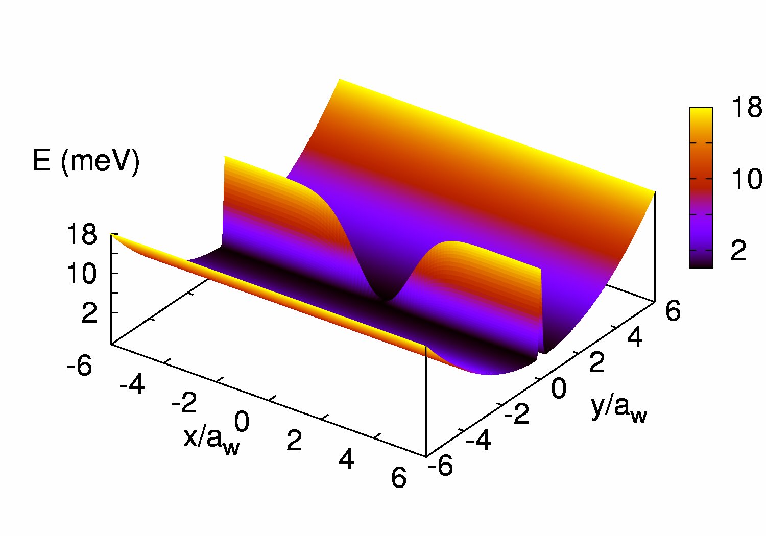
Figure 1: (Color online) Schematic illustration of the potential defining the window-coupled DW system. $\hbar\Omega_{0}=1.0$ meV, $B=0$ T, $a_{w}=33.74$ nm.

Figure 1 schematically illustrates the window-coupled DW system scaled by $a_{w}$. The embedded DW system is described by $V_{\rm DW}(\mathbf{r})=V_{\rm MB}(y)+V_{\rm CW}(x,y)$ that contains a middle barrier

$$V_{\rm MB}(y)=V_{0}\;{\rm exp}{(-\beta_{0}^{2}y^{2})}$$ (31)

with $V_{0}=18.0$ meV and $\beta_{0}=0.3$ nm^-1, as well as a coupling window potential

$$V_{\rm CW}(x,y)=-V_{0}\;{\rm exp}{(-\beta_{x}^{2}x^{2}-\beta_{y}^{2}y^{2})}.$$ (32)

The coupling constant $g_{0}^{l}a_{w}^{3/2}=60\ {\rm meV}$, and the contact size parameter $\delta_{x}^{l}=\delta_{y}^{l}=4.4\times 10^{-4}$ nm^-2

In the following calculations, the temperature of the reservoirs is fixed at $T=0.5$ K, and the states within the bias window before switching-on the coupling are assumed to be unoccupied. The coupling between the DW system and the leads is characterized by the switching rate $\gamma=1.0$ ps^-1, and the nonlocal coupling strength is fixed as $\Gamma^{l}=4g_{0}^{l}a_{w}^{3/2}/(\delta_{x}^{l}\delta_{y}^{l})^{1/2}=54.5$ meV$\cdot$nm². The bias voltage is fixed leading to a bias window $eV_{\rm bias}=\Delta\mu=0.9$ meV, and the extension parameter $\Delta=0.3$ meV is selected referring to a window of relevant states $\Delta_{E}=\Delta\mu+2\Delta=1.5$ meV.

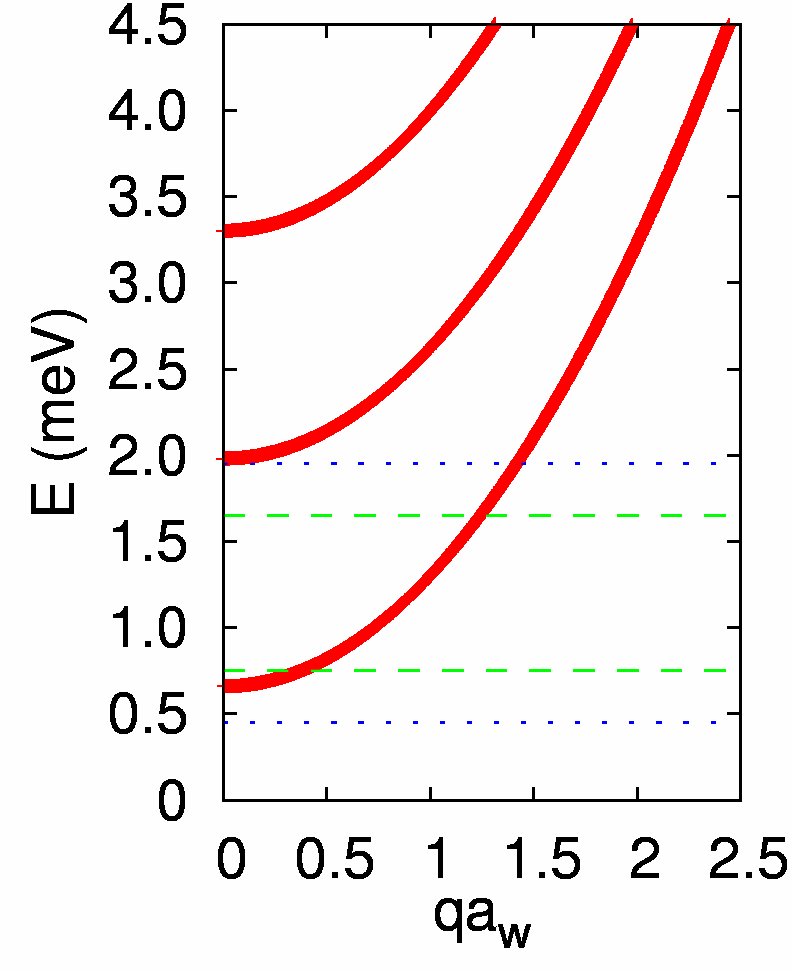
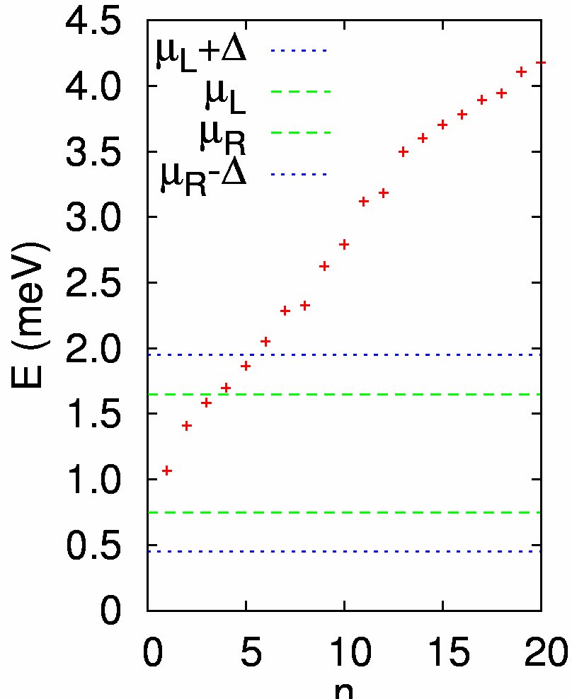
Figure 2: (Color online) Energy spectrum of the leads (solid red) versus wave number $q$ (left panel); and energy spectrum of the window-coupled DW system (cross dot) versus the SES number $n$ (right panel). Magnetic field $B=0.5$ T, and the chemical potentials in the the leads are $\mu_{L}=1.65\ {\rm meV}$ and $\mu_{R}=0.75\ {\rm meV}$ (dashed green) such that $\Delta\mu=0.9$ meV. The window of relevant states $\Delta_{E}=1.5$ meV is defined by the dotted blue lines.

The energy spectrum of the leads as a function of wave number $q$ scaled by $a_{w}^{-1}$ is shown in the left panel of Fig. 2. The bias window $\Delta\mu$ is located in the first subband, whereas the extended active bias window covers the evanescent modes below the first subband and the threshold of the second subband. The energy spectrum of the window-coupled DW system as a function of the single electron number $n$ is shown in the right panel of Fig. 2 containing five SESs in the window of relevant states $\Delta_{E}$; the three lowest states are in the bias window $\Delta\mu$ whereas the two highest states are in the upper extended window $[\mu_{L},\mu_{L}+\Delta]$.

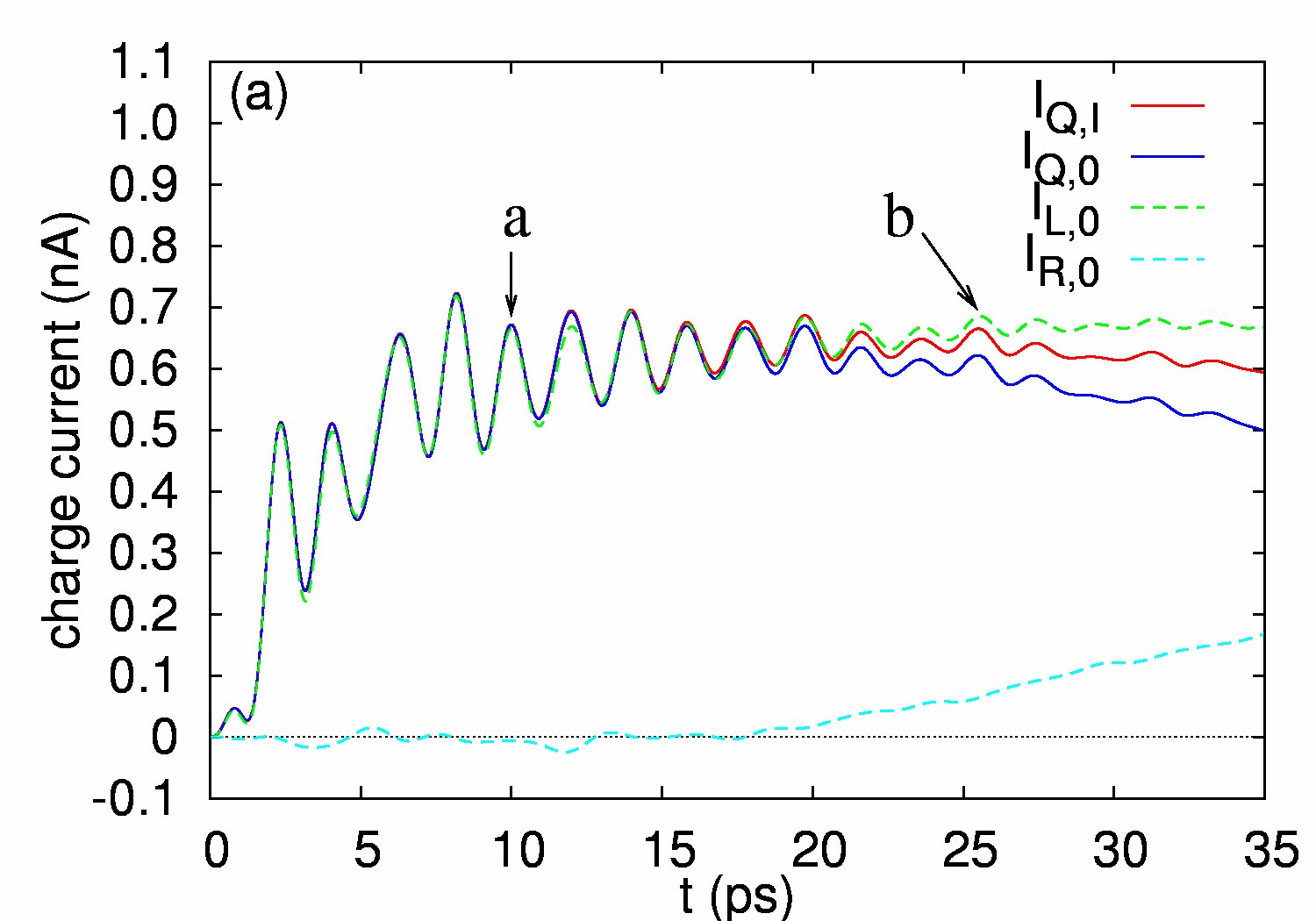
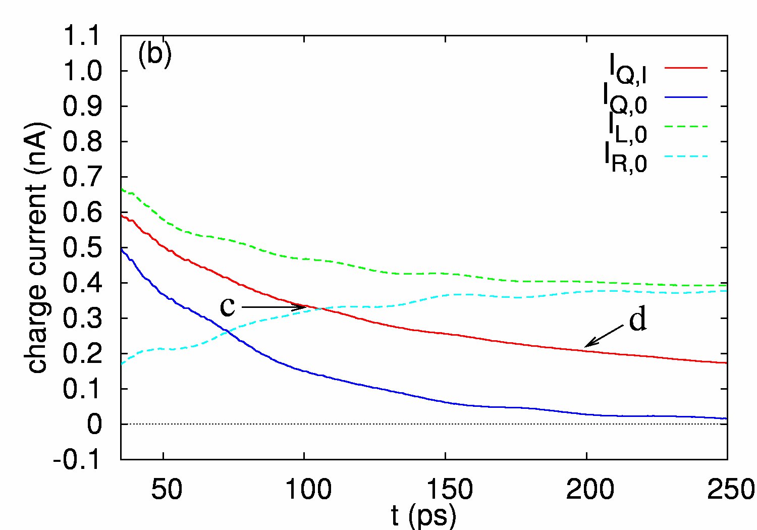
Figure 3: (Color online) The interacting net current $I_{Q,I}$ (solid red), the noninteracting net current $I_{Q,0}$ (solid blue), the noninteracting left current $I_{L,0}$ (dashed green), and the noninteracting right current $I_{R,0}$ (dashed light-blue) are plotted as a function of time: (a) short-time response; (b) long-time response. $B=0.5$ T, $L_{\rm w}=100$ nm, the coupling constant $g_{0}^{l}a_{w}^{3/2}=60\ {\rm meV}$, and the contact size parameters $\delta_{x}^{l}=\delta_{y}^{l}=4.4\times 10^{-4}$ nm^-2.

In Fig. 3, we show the time-dependent charge current for the case of magnetic field $B=0.5$ T with and without $e$-$e$ interaction, denoted by $I_{Q,I}$ and $I_{Q,0}$ respectively. The noninteracting left and the right currents are also presented for comparison, denoted by $I_{L,0}$ and $I_{R,0}$ respectively. We have selected $\beta_{x}=0.02$ nm^-1 and $\beta_{y}=\beta_{0}$ such that the length of the coupling window $L_{\rm w}$ is $100$ nm. In addition, the coupling constant is $g_{0}^{l}a_{w}^{3/2}=60\ {\rm meV}$ and the contact size parameters are $\delta_{x}^{l}=\delta_{y}^{l}=4.4\times 10^{-4}$ nm^-2 such that the coupling strength $\Gamma^{l}=54.5$ meV$\cdot$nm² and the effective lengths of the system-lead coupling potential are $L_{c,x}^{l}=L_{c,y}^{l}\approx 95$ nm. Below we shall show that the time-dependent charge current manifests different transport mechanisms in the short-time and the long-time response.

In the short-time response regime, shown in Fig. 3(a), the time-dependent charge current is increased and manifests rapid oscillation with period $\tau_{s}\approx 1.9$ ps exhibiting quantum interference dominant features. In this regime, the noninteracting approach could be a good approximation for analyzing the transient time-dependent transport properties. In this short-time regime, the interacting and the noninteracting currents are almost the same before $20$ ps with negligible right charge current implying effective charging and quantum interferance dominant transport feature. The right charge current is significantly increased after $20$ ps. At around $t=35$ ps, the difference between the interacting and noninteracting currents becomes $0.1$ nA (the Coulomb correction is $\sim 10\%$), and the right charge current is increased to $0.18$ nA.

In the long-time response shown in Fig. 3(b), the charge current displays slow quasi-periodic oscillation with period $\tau_{l}\approx 39$ ps approaching a steady current. The slow oscillation behavior in the time-dependent current implies that the quantum interference feature is suppressed whereas the Coulomb interaction effect is enhanced. At time $t=250$ ps, the interacting steady current ($\sim 0.17$ nA) is much higher than the noninteracting steady current ($\sim 0.015$ nA). The mean charge of the DW system is monotonically increased in time (not shown),Vidar2010 and the mean charge of the interacting MES ($\sim 0.8e$) is approximately twice that of the steady mean charge of the noninteracting MES ($\sim 0.4e$). This indicates that the empty-state initial condition ensures that the Coulomb interaction facilitates to drag the electron dwelling in the DW system through the window of relevant states, and thus enhances the steady current.

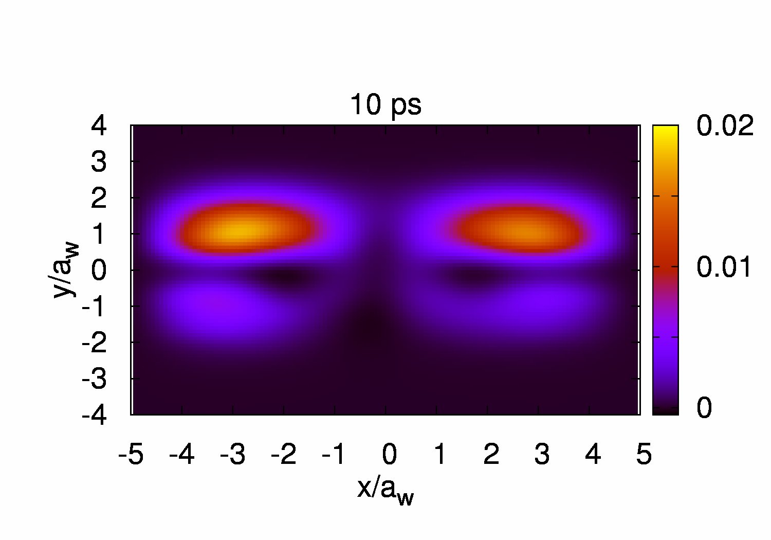
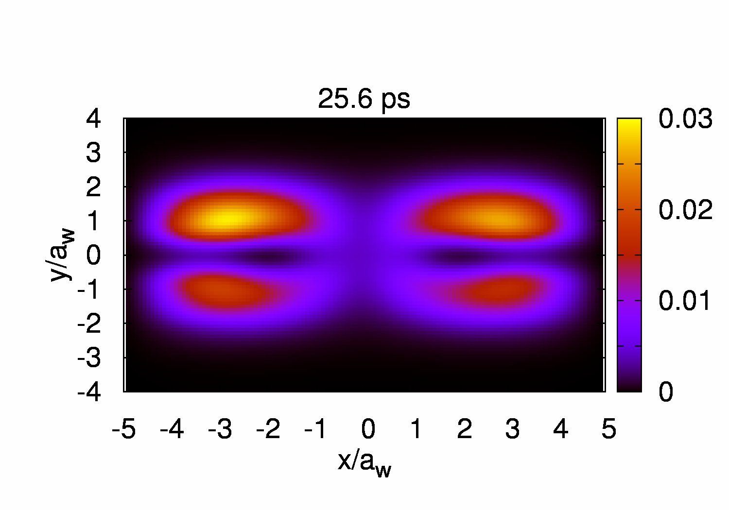
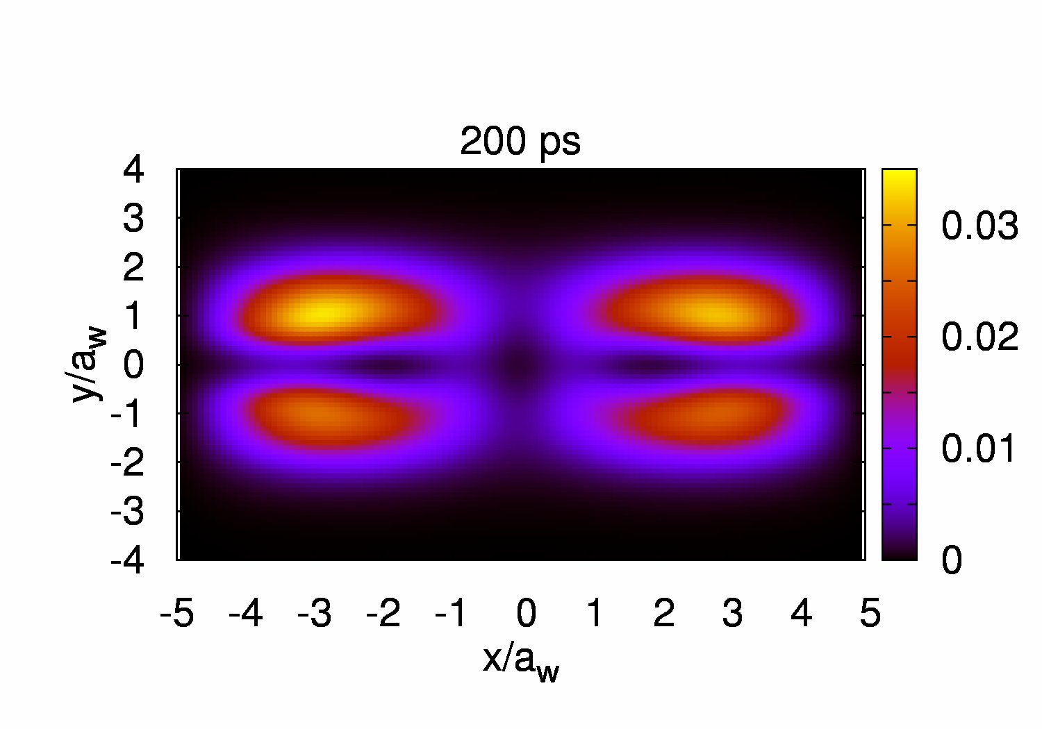
Figure 4: (Color online) The many-electron charge density for the noninteracting (left panel) and interacting system (right panel) for $B=0.5$ T. The other parameters are the same as Fig. 3.

In order to get better understanding on the transient dynamical transport, we present the spatial distribution of the many-electron charge at $t=10$, $25.6$, $100$, and $200$ ps in Fig. 4, labeled by $\bf{a}$-$\bf{d}$ in Fig. 3, respectively. When the system-lead coupling is switched-on with forward bias, the electrons are incident from the left lead into the system with transversely symmetric distribution (not shown). At around $t\simeq 10$ ps, the electrons located in the lower wire favorite to make inter-wire backward scattering to the upper wire, exhibiting a fully quantum mechanical feature. Later on, the electrons perform an opposite inter-wire backward scattering feature to the lower wire at $t\simeq 25$ ps, and this feature is only slightly enhanced by the Coulomb interaction. However, in the long-time response regime, the inter-wire scattering forward and backward effects are both enhanced. At around $t=100-200$ ps, the noninteracting window-coupled DW forms a quasi-isolated four cavities, the window coupling effect is significantly enhanced by the Coulomb interaction. It is interesting that the electron can form a quasibound state in the coupling window at $t\simeq 200$ ps. When the DW system approaches steady-state transport in the long-time response regime, the total charge in the system is $0.4e$ for noninteracting and $0.8e$ for interacting DW system exhibiting significant charge accumulation behavior.

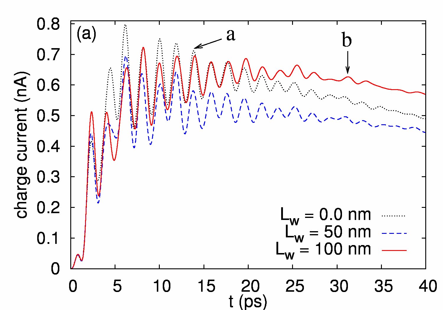
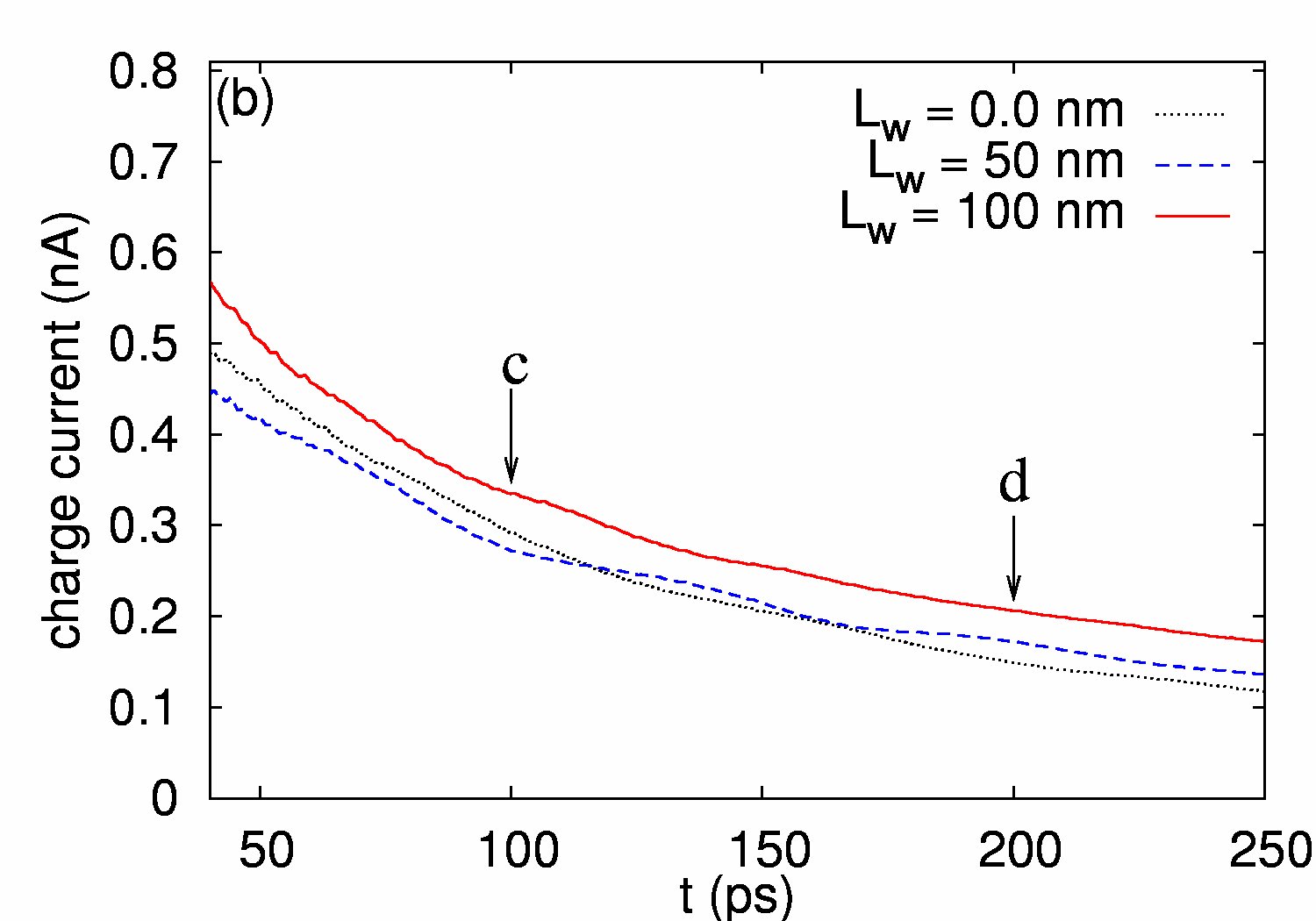
Figure 5: (Color online) The interacting net current $I_{Q,I}$ versus time for $L_{\rm w}=0$ (dotted black), $50$ (dashed blue), and $100$ nm (solid red): (a) short-time response; (b) long-time response for $B=0.5$ T. The other parameters are the same as Fig. 3.

In Fig. 5, we show the interacting net charge current as a function of time for the case of magnetic field $B=0.5$ T with different size of coupling window $L_{\rm w}=0$ (dotted black), $50$ (dashed blue), and $100$ nm (solid red). In the short-time response regime, shown in Fig. 5(a), the quantum interference dominates the time-dependent charge current feature with rapid oscillation. The oscillation amplitude and frequency of the time-dependent charge current remain similar for the cases with different window size, this similarity is because the quantum interference oscillation behavior is mainly due to the multiple scattering in the transport direction, and interference of subbands in the semi-infinite leads. In the transient switching-on regime $t\leq 0.5$ ps, the charge current for both the cases of short $L_{\rm w}=50$ nm and long window $L_{\rm w}=100$ nm are similar to the case without a window $L_{\rm w}=0.0$ nm exhibiting the response time of the system from an isolated system to an open system. Later on, the charge current for the case of short window is suppressed by $0.4$ nA, while the charge current is enhanced for the case of long window by $0.8$ nA. It should be noted that this quantitative feature is different when the $e$-$e$ interaction effect is ignored, in which the charge current is almost the same for the cases without window $L_{\rm w}=0.0$ nm and long window $L_{\rm w}=100$ nm, however the charge current is suppressed by $1$ nA for the case of short window $L_{\rm w}=50$ nm (not shown).

In the long-time response regime, shown in Fig. 5(b), the time-dependent charge current displays slow oscillations and approaches to a steady current within $0.1-0.2$ nA. It is shown that the steady current is enhanced for the case of long window $L_{\rm w}=100$ nm due to the Coulomb interaction. However, the Coulomb interaction for the case of short widow is not significant on the time-dependent charge current in comparison with the pure finite length DW system without window coupling. When the Coulomb interaction is ignored, the steady currents of the short and the long window are both suppressed (not shown). This demonstrates again the dynamics of the time-dependent charge current in the long-time response regime is significantly affected by the Coulomb interaction.

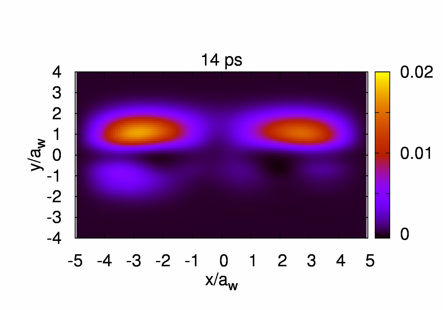
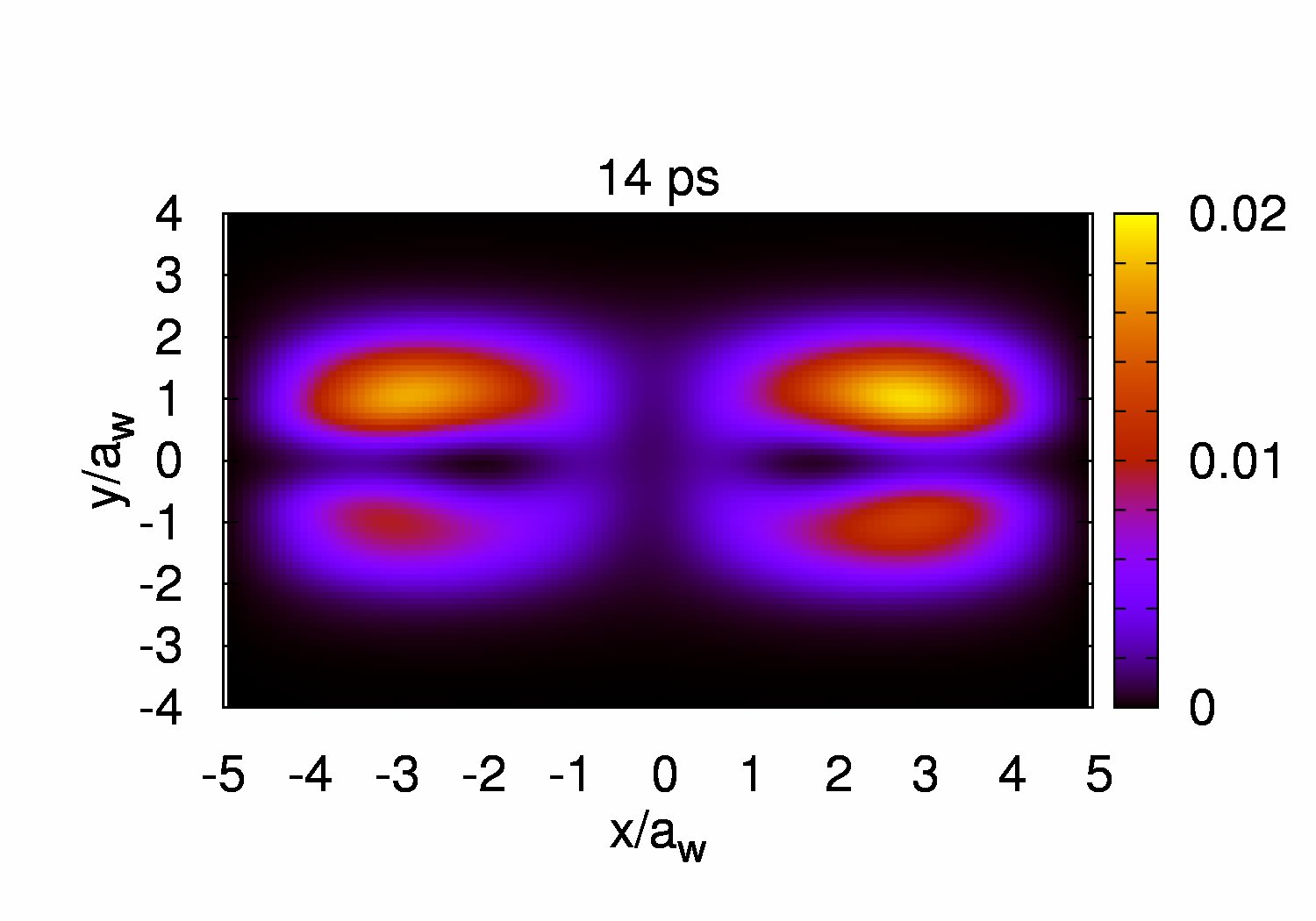
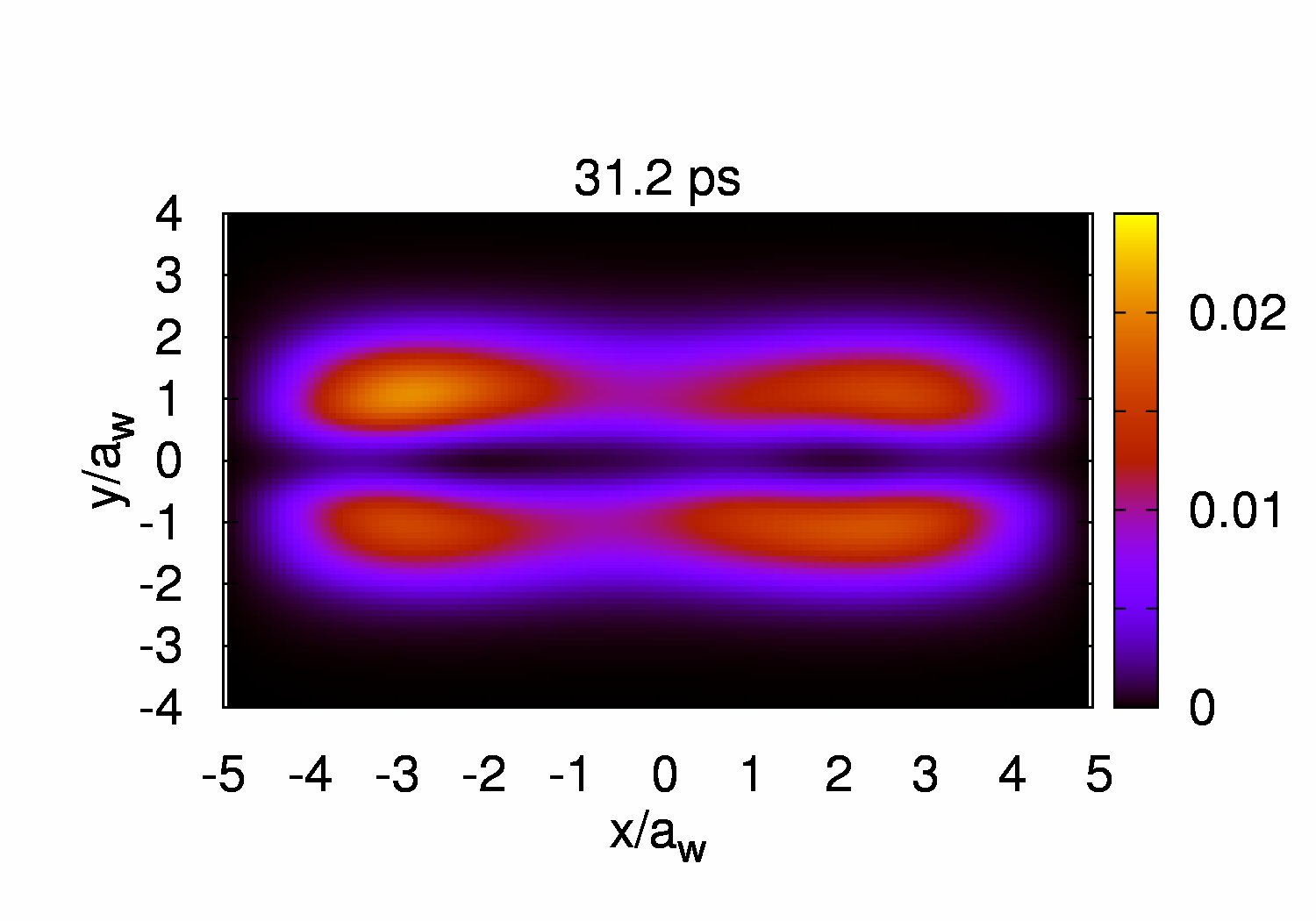
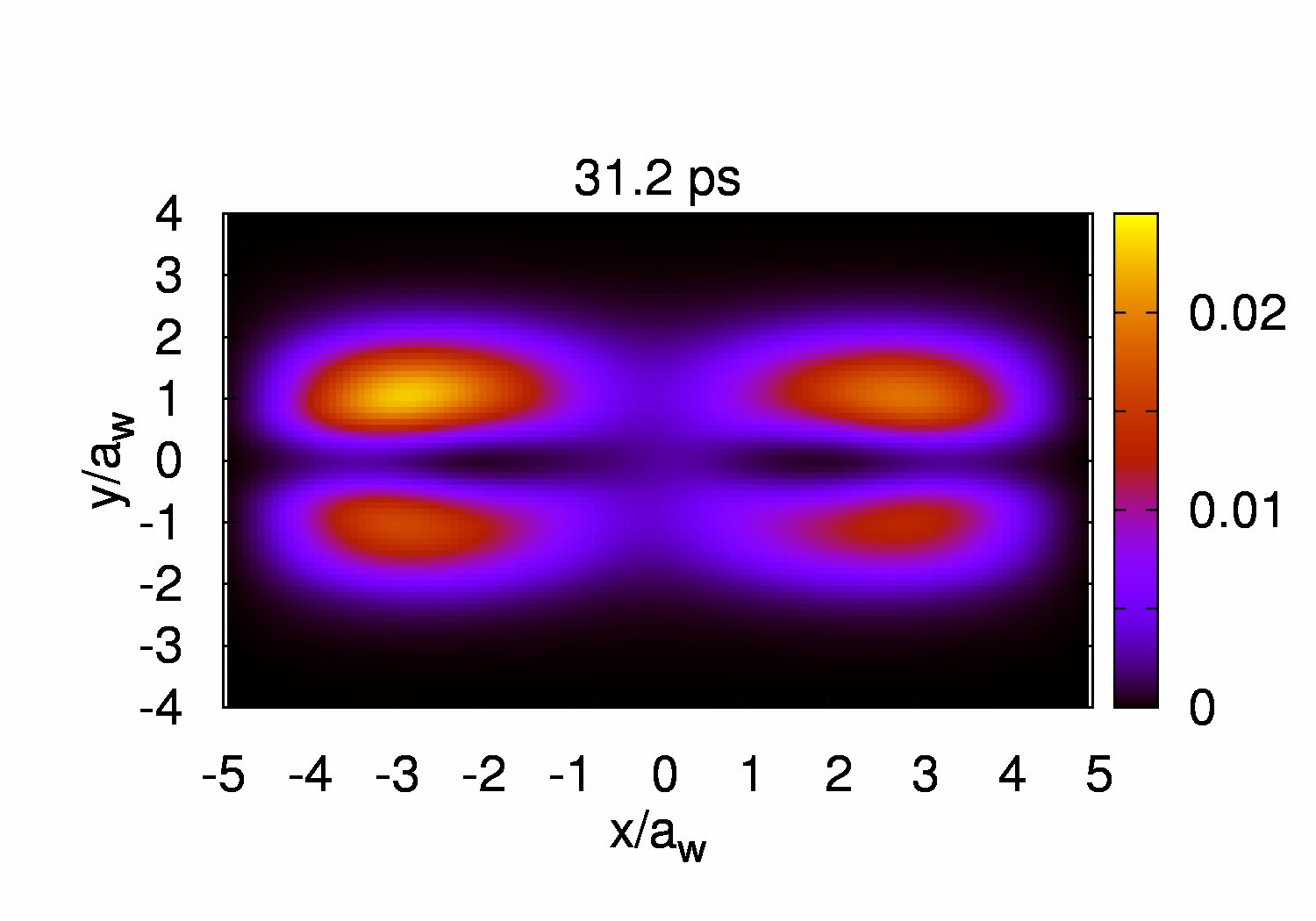
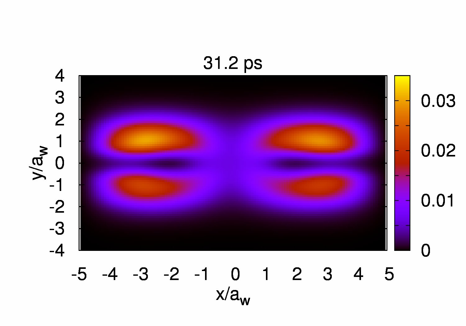
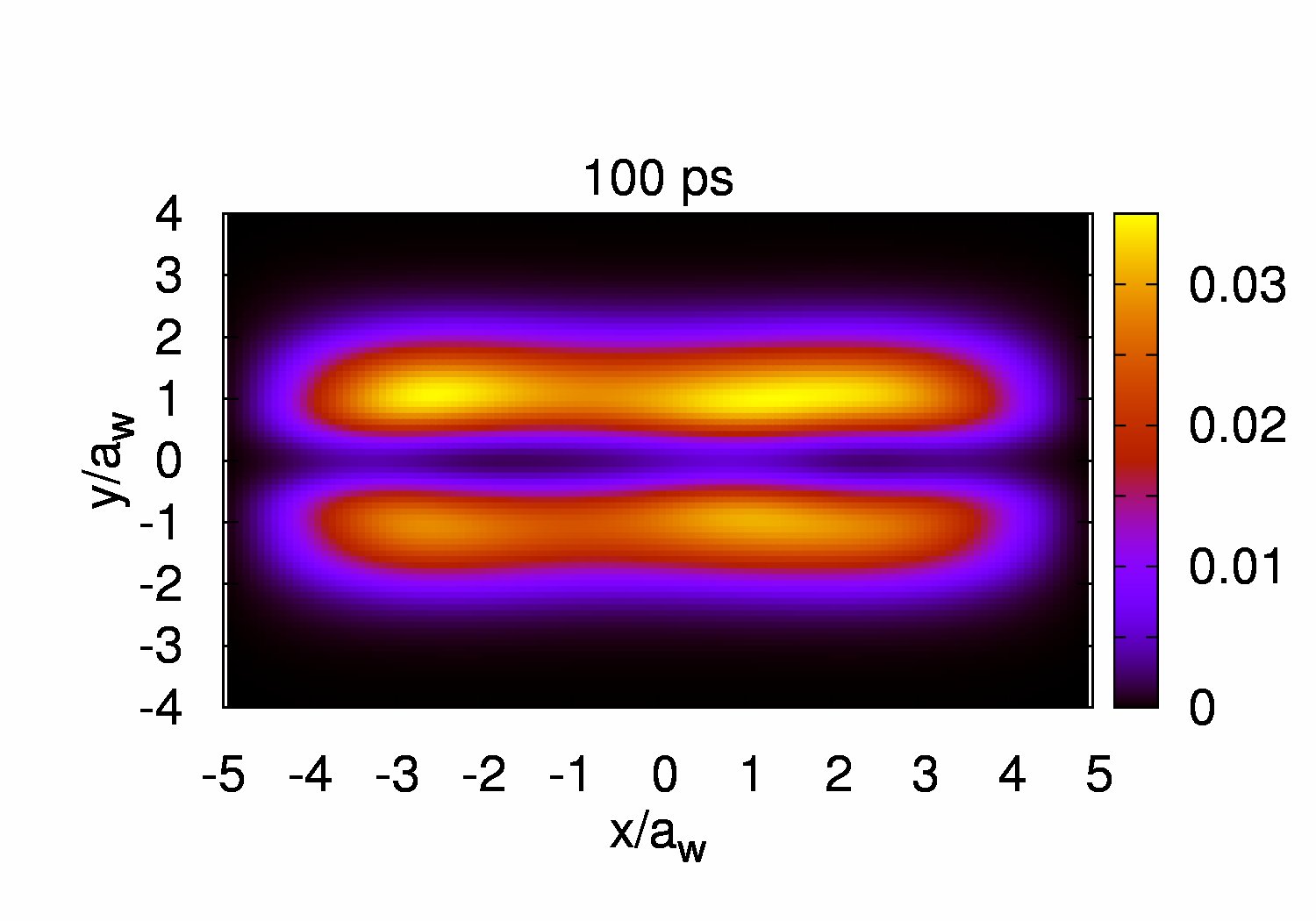
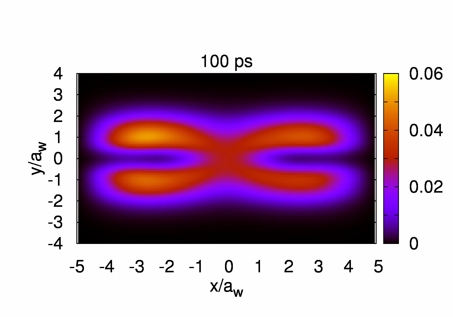
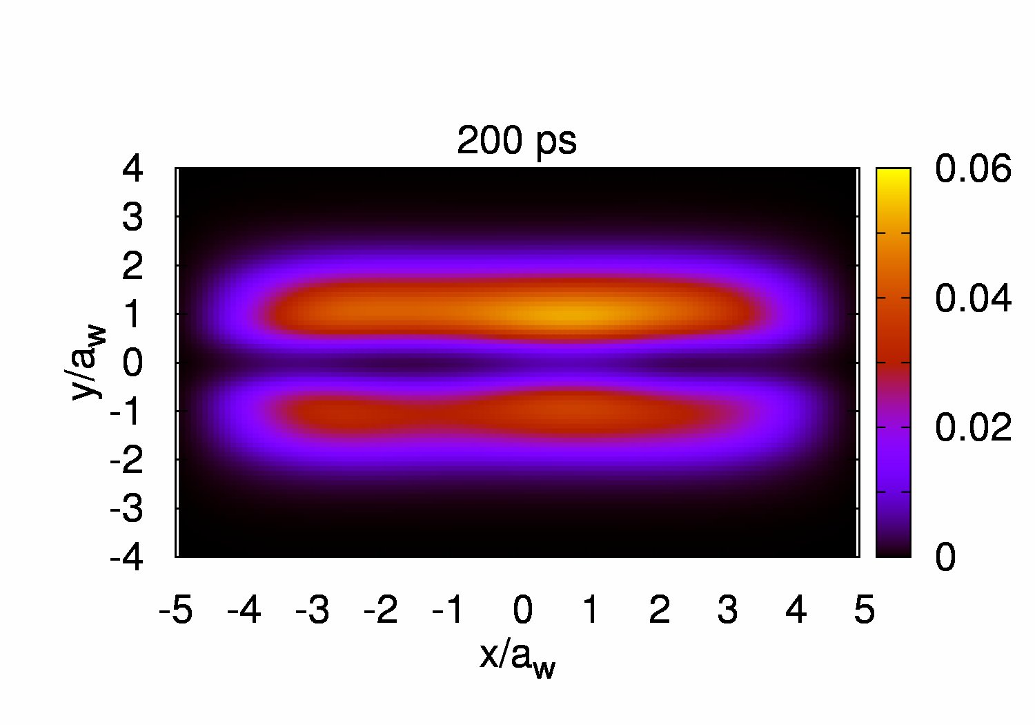
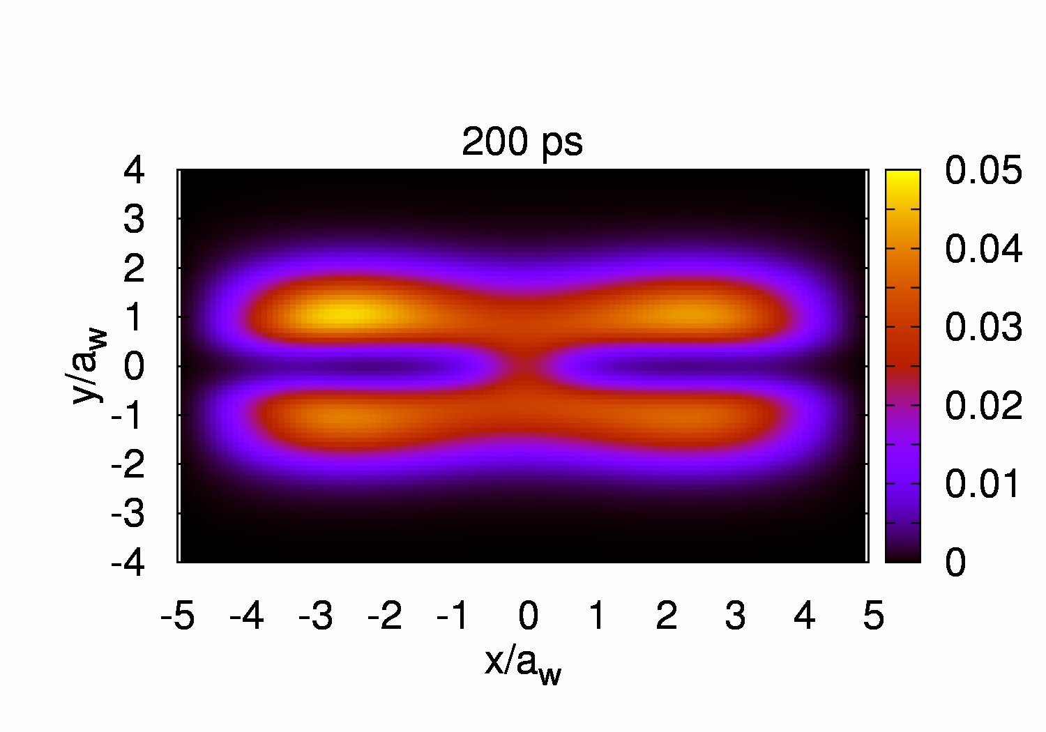
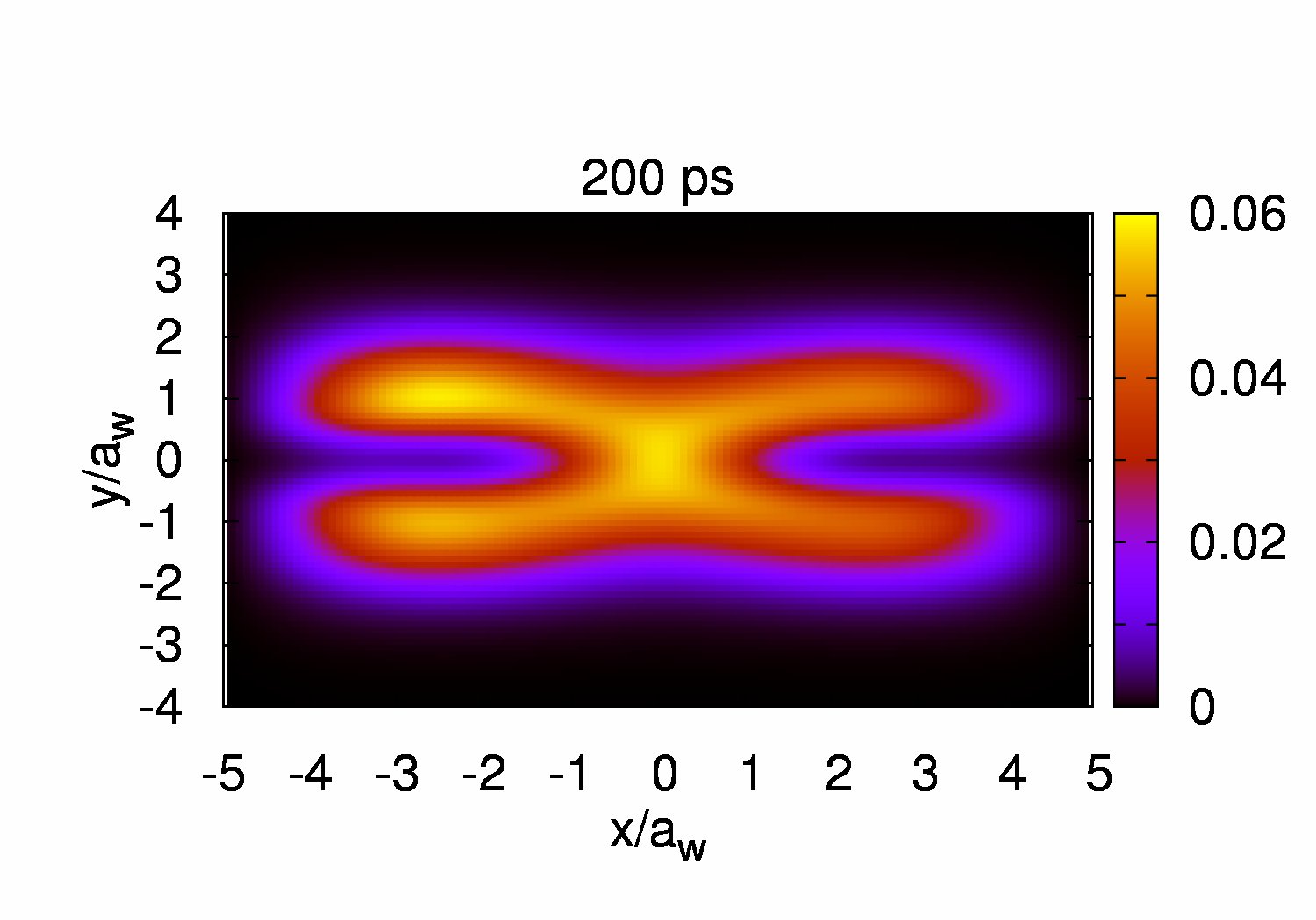
Figure 6: (Color online) The spatial distribution of the interacting many-electron charge density with different coupling window: $L_{\rm w}=0.0$ nm (left), $L_{\rm w}=50$ nm (middle), and $L_{\rm w}=100$ nm (right) at time $t=14$, $31.2$, $100$, and $200$ ps. $B=0.5$ T, and the other parameters are the same as Fig. 3.

To investigate how the window size affects the transport dynamics, in Fig. 6 we present the spatial distribution of the many-electron charge at $t=14$, $31.2$, $100$, and $200$ ps, labeled by $\bf{a}$-$\bf{d}$ in Fig. 5, respectively. It is clearly seen that, for both short and long window, the electrons perform inter-wire backward scattering in the short-time response regime (say, $t=14$ and $31.2$ ps), while the electrons are allowed to perform inter-wire forward scattering in the long-time response regime (say, $t=100$ and $200$ ps). This means that the former quantum interference dominant short-time response regime, the electrons favor the inter-wire backward scattering; while the latter Coulomb interaction dominant long-time response regime, the electrons favor inter-wire forward scattering. The many-electron charge density is monotonically increased in time. Furthermore, it is demonstrated that increasing window size can enhance not only the inter-wire scattering feature, but also the local charge accumulation at the coupling window.

IV Concluding Remarks

To conclude, we have performed a numerical calculation of the time-dependent electric current and spatial charge distribution through a window-coupled parallel double quantum wire system based on GQME formalism including the electron-electron Coulomb interaction with the “exact diagonalization” method, and without resorting to the commonly used Markovian approximation. We have analyzed transient currents and their dependence on various parameters of the system with a certain initial configuration and time-dependent switching-on coupling to the leads. For a given coupling window, we have demonstrated time-dependent transport properties of the noninteracting and the interacting DW systems. Applying an appropriate magnetic field, we have found a short-time response regime dominated by quantum interference and inter-wire backward scattering. Moreover, the Coulomb correlation is significantly enhanced in the long-time response regime,Vidar2010 and the inter-wire forward scattering through the coupling window dominates the dynamical transport properties. The conceived mesoscale window-coupled DW system could serve as an elementary quantum device for sensitive spectroscopy tools for electrons and quantum information processing by controlling the coupling window and the applied magnetic field.

- (1) R. Schuster et al., Nature (London) 385, 417 (1997).
- (2) M. Avinun-Kalish et al., Nature (London) 436, 529 (2005).
- (3) C.-S. Tang, W, W. Yu, and V. Gudmundsson, Phys. Rev. B 72, 195331 (2005).
- (4) V. Gudmundsson and C.-S. Tang, Phys. Rev. B 74, 125302 (2006).
- (5) P. A. Orellana, F. Domínguez-Adameb, E. Diezc, Physica E 35, 126 (2006).
- (6) O. Valsson, C.-S. Tang, and V. Gudmundsson, Phys. Rev. B 78, 165318 (2008).
- (7) K.-W. Chen and C.-R. Chang, Phys. Rev. B 78, 235319 (2008).
- (8) C. C. Eugster and J. A. del Alamo, Phys. Rev. Lett. 67, 3586 (1991).
- (9) D. M. Schroer, A. K. Huttel, K. Eberl, S. Ludwig, M. N. Kiselev, and B. L. Altshuler, Phys. Rev. B 74, 233301 (2006).
- (10) J. C. Barbosa and P. N. Butcher, Superlatt. Microstruct. 22, 325 (1997).
- (11) S. V. Korepov and M. A. Liberman, Physica B 109, 92 (2002).
- (12) J.-R. Shi and B.-Y. Gu, Phys. Rev. B 55, 9941 (1997).
- (13) A. Ramamoorthy, J. P. Bird, and J. L. Reno, Appl. Phys. Lett. 89, 013118 (2006).
- (14) C.-S. Tang and V. Gudmundsson, Phys. Rev. B 74, 195323 (2006).
- (15) S. Mukamel, Phys. Rev. Lett. 90, 170604 (2003).
- (16) T. Monnai, Phys. Rev. E 72, 027102 (2005).
- (17) M. Esposito and S. Mukamel, Phys. Rev. E 73, 046129 (2006).
- (18) G. E. Crooks, Phys. Rev. A 77, 034101 (2008).
- (19) J. Rammer, A. L. Shelankov, and J. Wabnig, Phys. Rev. B 70, 115327 (2004).
- (20) J. Y. Luo, X.-Q. Li, and Y. J. Yan, Phys. Rev. B 76, 085325 (2007).
- (21) S. Welack, M. Esposito, U. Harbola, and S. Mukamel, Phys. Rev. B, 77, 195315 (2008).
- (22) P. Lambropoulos et al., Rep. Prog. Phys. 63, 455 (2000).
- (23) N. G. Van Kampen, Stochastic Processes in Physics and Chemistry, 2nd Ed. (North-Holland, Amsterdam, 2001).
- (24) U. Harbola, M. Esposito, and S. Mukamel, Phys. Rev. B 74, 235309 (2006).
- (25) S. A. Gurvitz and Y. S. Prager, Phys. Rev. B 53, 15932 (1996).
- (26) A. Braggio, J. König, and R. Fazio, Phys. Rev. Lett., 96, 026805 (2006).
- (27) C. Emary, D. Marcos, R. Aguado, and T. Brandes, Phys. Rev. B 76, 161404(R) (2007).
- (28) A. Bednorz and W. Belzig, Phys. Rev. Lett. 101, 206803 (2008).
- (29) V. Gudmundsson, C. Gainar, C.-S. Tang, V. Moldoveanu, and A. Manolecu, New J. Phys. 11, 113007 (2009).
- (30) E. Vaz and J. Kyriakidis, Phys. Rev. B 81, 085315 (2010).
- (31) C. S. Tang and C. S. Chu, Phys. Rev. B 53, 4838 (1996).
- (32) C. S. Tang, Y. H. Tan, and C. S. Chu, Phys. Rev. B 67, 205324 (2003)
- (33) P. Sharma and C. Chamon, Phys. Rev. Lett. 87, 096401 (2001).
- (34) C. S. Tang and C. S. Chu, Phys. Rev. B 60, 1830 (1999).
- (35) G. Platero and R. Aguado, Phys. Rep. 395, 1 (2004).
- (36) D. C. Guhr, D. Rettinger, J. Boneberg, A. Erbe, P. Leiderer, and E. Scheer, Phys. Rev. Lett. 99, 086801 (2007).
- (37) S. Sasaki, S. Kang, K. Kitagawa, M. Yamaguchi, S. Miyashita, T. Maruyama, H. Tamura, T. Akazaki, Y. Hirayama, and H.Takayanagi, Phys. Rev. B 73, 161303 (2006).
- (38) C. S. Tang, A. G. Mal’shukov, and K. A. Chao, Phys. Rev. B 71, 195314 (2005).
- (39) A. F. Amin, G. Q. Li, A. H. Phillips, and U. Kleinekathöfer, Eur. Phys. J. B 68, 103 (2009).
- (40) N. Sai, N. Bushong, R. Hatcher, and M. Di Ventra, Phys. Rev. B 75, 115410 (2007).
- (41) B. Wang, Y. Xing, L. Zhang, and J. Wang, Phys. Rev. B 81, 121103(R) (2010).
- (42) V. Moldoveanu, A. Manolescu, and V. Gudmundsson, New J. Phys. 11, 073019 (2009).
- (43) C. Yannouleas and U. Landman, Rep. Prog. Phys. 70, 2067 (2007), and references therein.
- (44) H.-P. Breuer and F. Petruccione, The Theory of Open Quantum Systems (Oxford University Press, Oxford, 2002).
- (45) M. Esposito, U. Harbola, and S. Mukamel, Rev. Mod. Phys. 81, 1665 (2009).
- (46) F. Haake, Phys. Rev. A 3, 1723 (1971).
- (47) F. Haake, in Quantum Statistics in Optics and Solid-state Physics, edited by G. Hohler and E.A. Niekisch, Springer Tracts in Modern Physics Vol. 66 (Springer, Berlin, Heidelberg, New York, 1973), p. 98.
- (48) V. Gudmundsson, C.-S. Tang, O. Jonasson, V. Moldoveanu, and A. Manolescu, Phys. Rev. B 81, 205319 (2010).