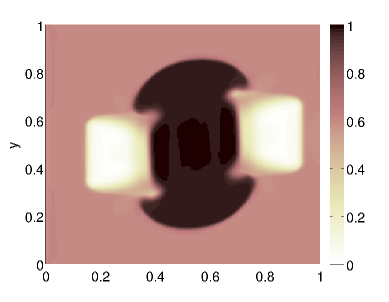
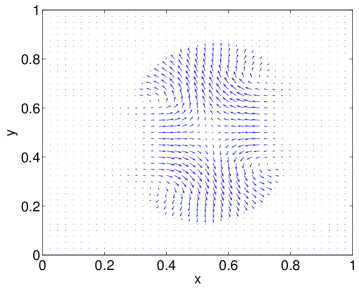
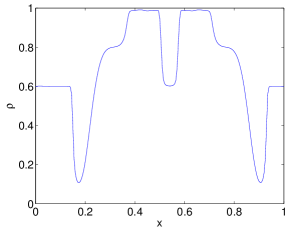
Numerical simulations of the Euler system with congestion constraint

Pierre Degond111Université de Toulouse; UPS, INSA, UT1, UTM; Institut de Mathématiques de Toulouse; F-31062 Toulouse, France. Email: pierre.degond@math.univ-toulouse.fr, Jiale Hua222CNRS; Institut de Mathématiques de Toulouse UMR 5219; F-31062 Toulouse, France. Email: jiale.hua@math.univ-toulouse.fr, Laurent Navoret333CNRS; Institut de Mathématiques de Toulouse UMR 5219; F-31062 Toulouse, France. Email: laurent.navoret@math.univ-toulouse.fr
Abstract

In this paper, we study the numerical simulations for Euler system with maximal density constraint. This model is developed in [9, 17] with the constraint introduced into the system by a singular pressure law, which causes the transition of different asymptotic dynamics between different regions. To overcome these difficulties, we adapt and implement two asymptotic preserving (AP) schemes originally designed for low Mach number limit [16, 18] to our model. These schemes work for the different dynamics and capture the transitions well. Several numerical tests both in one dimensional and two dimensional cases are carried out for our schemes.

Key words: Finite volume scheme, Congestion, Asymptotic-Preserving schemes, All-speed flows, Pressureless Gas Dynamics

1 Introduction

Several models involve congestion constraints: concentration constraints occur in multi-phase flow modeling [12], maximal density constraints occur when dealing with finite-size interactive agents in herds of gregarious mammals [17], in cars or pedestrians flows [9, 10, 3], flux constraints occur for supply chains [2],… The dynamics in congested regions strongly differ from the dynamics dynamics in free regions. To study the transitions between congested and free regions, a general methodology was first carried out in [12] for multiphase flows and later on generalized to traffic [9] or herding problems [17]: the stiffness of the constraint leads to a singular perturbation problem and then the limit problem provides a clear cut-off between the two dynamics. In this paper, we will consider the Euler system with a singular pressure which encodes a maximal density constraint. As in [17], the limit problem is a two-phase model between incompressible regions, where the maximal density is reached, and compressible regions for lower densities. Our goal is to provide numerical schemes that are able to capture this limit problem and these transitions. In this paper, we adapt and compare two numerical methods presented in [18] and in [16] for the low Mach number limit.

A lot of efforts have been made to devise numerical schemes valid for all Mach numbers, that is, for both compressible and incompressible flows. They avoid the switch between different methods, when different Mach numbers occur in different sub-domains. Among such schemes, one approach is the extension of compressible conservative methods to incompressible flows thanks to preconditioning techniques [37, 20, 19, 28]. The second approach is the extension of incompressible methods to compressible flows and leads to pressure correction methods on staggered grids [21] and their conservative versions [33, 6, 38]. Their adaptation to the conservative frameworks has led to time semi-implicit schemes : the implicit discretization of the fluxes (the mass flux and the pressure part of the momentum flux are taken implicitly) is combined with the resolution of the elliptic equation satisfied by the pressure. The implicit treatment of the pressure flux ensures stability with respect to the propagation of fast acoustic waves in the low-Mach number limit but induces a lot of diffusion. We can cite numerous works following this methodology [25, 39, 30, 31, 34]. The methods we consider in this paper are among the simplest ones: the scheme in [18] is a semi-implicit scheme with a division of the pressure into explicit and implicit parts and in [16], the Gauge decomposition of the momentum enables the hydrostatic pressure to act only on the divergence-free part of the momentum. The former method will be called in the present paper the Direct method, while the Gauge method will refer to the latter.

The purpose of this paper is to present simple variants of the Direct [18] and the Gauge method [16], that are able to handle congestion problems. As announced above, they are designed to solve the isentropic Euler system supplemented by a pressure law p(ρ)𝑝𝜌p(\rho), which is singular as the density ρ𝜌\rho approaches a maximal density denoted ρsuperscript𝜌\rho^{\ast}. A small parameter ε𝜀\varepsilon is introduced to control the stiffness of this maximal density constraint: the rescaled pressure εp(ρ)𝜀𝑝𝜌\varepsilon p(\rho) is of order O(1)𝑂1O(1) in congested regions ρρsimilar-to𝜌superscript𝜌\rho\sim\rho^{\ast} and of order O(ε)𝑂𝜀O(\varepsilon) in low density regions ρ<ρ𝜌superscript𝜌\rho<\rho^{\ast}. In the limit ε0𝜀0\varepsilon\rightarrow 0, the system leads to a two-phase model: the incompressible Euler system in maximal density domains and the pressureless gas dynamics system for uncongested densities domains. This asymptotic model was first proposed and studied in [12, 8] in a one-dimensional framework. However, this asymptotic model is only partially defined since transmission conditions at the interfaces between the two phases are lacking. Besides, unless one-dimensional solutions can be provided (see [12] and appendix A), their extensions to the two-dimensional case are open problems (especially the dynamics of two colliding congested domains). In this context, asymptotic preserving scheme is a good tool for this problem.

The Direct and the Gauge methods are called asymptotic-preserving (AP) since they are uniformly consistent with the low-Mach number limit. Besides, they are also uniformly stable. These methods are expected to capture both the compressible and the incompressible dynamics arising in the congestion limit of the Euler system with the maximal density constraint. In this case, such AP numerical schemes are very powerful since they provide the dynamics of transitions, for which analytical results may be lacking. Moreover, they enable us to avoid dealing with physical and numerical interface tools, such as front-tracking [36] or volume-of-fluid methods [23]. Unlike these tracking methods, ours are front-capturing methods and then share some analogies with level-set [32] and diffusive interface methods [1]: like level-set method, the dynamics of the transition are implicitly embodied in the dynamics of an auxiliary function which here is the density and like the diffusive interface methods, the sharp interface is viewed as the limit of the smooth transitions of the perturbation problem.

The Direct method cannot be directly applied to the congestion problem. Indeed, in [18], the pressure p(ρ)𝑝𝜌p(\rho) is splitted into an explicit part p0(ρ)subscript𝑝0𝜌p_{0}(\rho) and an implicit part p1(ρ)subscript𝑝1𝜌p_{1}(\rho) in order to keep some numerical diffusion and avoid numerical oscillations. For the singular congestion pressure-law, we modify this splitting, such that it still ensures the stability of the scheme. Besides, it ensures the consistency of the explicit part of the scheme with the limit pressureless gas dynamics in the low density regions. Indeed, the pressureless gas dynamics system is weakly hyperbolic and there is no uniqueness of the entropic solution [11]. Then, keeping an explicit pressure p0(ρ)subscript𝑝0𝜌p_{0}(\rho) makes the asymptotic numerical solutions consistent with the good entropic solutions. For the same reasons, this pressure splitting is introduced into the Gauge method.

The AP property of the two methods for the congested Euler system is demonstrated for the congested domains. This analysis is hard to extend to coexistent congested and uncongested regions since the dynamics of the interfaces between the different regions is not explicitly implemented into the schemes. However, several numerical test-cases provides numerical evidence of the AP property. Comparisons of the two schemes are also carried out and different behaviours of the schemes at the interfaces are measured.

The paper is organized as follows. In section 2, we introduce the Euler system with the maximal density constraint. To have some basic idea of the solution, we give its formal asymptotic limit. In section 3, we describe the time semi-discretization of the Direct and Gauge schemes. The fully space and time discretizations are exposed in section 4, in one dimensional setting: they are based on the centered Rusanov scheme, also called the local Lax-Friedrichs scheme [27]. The two dimensional setting is quite similar. Therefore, we present it in the appendix. Finally, numerical simulations are performed in section 5 to compare the two schemes: several test cases in the one dimensional setting and one case in the two dimensional setting. Two appendices close this study: we describe one-dimensional solutions and the two dimensional discretizations.

2 The Euler system with congestion and its asymptotic limit

2.1 The model

We consider the two-dimensional Euler system:

tρ+𝒙𝒒=0,subscript𝑡𝜌subscript𝒙𝒒0\displaystyle\partial_{t}\rho+\nabla_{\boldsymbol{x}}\cdot\boldsymbol{q}=0, (1)
t𝒒+𝒙(𝒒𝒒ρ)+𝒙p(ρ)=0,subscript𝑡𝒒subscript𝒙tensor-product𝒒𝒒𝜌subscript𝒙𝑝𝜌0\displaystyle\partial_{t}\boldsymbol{q}+\nabla_{\boldsymbol{x}}\cdot\left(\frac{\boldsymbol{q}\otimes\boldsymbol{q}}{\rho}\right)+\nabla_{\boldsymbol{x}}p(\rho)=0, (2)

where ρ(𝒙,t)𝜌𝒙𝑡\rho(\boldsymbol{x},t)\in\mathbb{R} denotes the mass density, 𝒒=ρ𝒖(𝒙,t)2𝒒𝜌𝒖𝒙𝑡superscript2\boldsymbol{q}=\rho\boldsymbol{u}(\boldsymbol{x},t)\in\mathbb{R}^{2} is the momentum field depending on the position 𝒙2𝒙superscript2\boldsymbol{x}\in\mathbb{R}^{2} and the time t>0𝑡0t>0. The pressure p(ρ)𝑝𝜌p(\rho) is an increasing function such that p(ρ)ργsimilar-to𝑝𝜌superscript𝜌𝛾p(\rho)\sim\rho^{\gamma} for densities ρ1much-less-than𝜌1\rho\ll 1 and p(ρ)+𝑝𝜌p(\rho)\rightarrow+\infty as ρ𝜌\rho tends to the congestion density ρsuperscript𝜌\rho^{\ast}. In the following, we will consider the function:

p(ρ)=1(1ρ1ρ)γ,γ>0.formulae-sequence𝑝𝜌1superscript1𝜌1superscript𝜌𝛾𝛾0p(\rho)=\frac{1}{\left(\frac{1}{\rho}-\frac{1}{\rho^{\ast}}\right)^{\gamma}},\quad\gamma>0. (3)

This pressure prevents the density from exceeding the congestion density. A variant is the van der Waals equation of state [22]. The operators 𝒙subscript𝒙\nabla_{\boldsymbol{x}} and 𝒙\nabla_{\boldsymbol{x}}\cdot are the gradient and the divergence of vector fields or tensor. For two vectors 𝒂𝒂\boldsymbol{a} and 𝒃𝒃\boldsymbol{b}, 𝒂𝒃tensor-product𝒂𝒃\boldsymbol{a}\otimes\boldsymbol{b} denotes the tensor product.

This model already appears in [17] with the additional constraint: 𝒒/ρ=𝒖𝕊1𝒒𝜌𝒖superscript𝕊1\boldsymbol{q}/\rho=\boldsymbol{u}\in\mathbb{S}^{1}. In this paper, we focus on the pressure singularity and the corresponding numerical schemes.

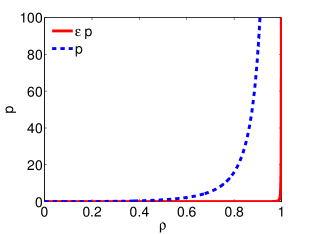
The singular pressure induces two different dynamics: for regions with densities near ρsuperscript𝜌\rho^{\ast}, the pressure takes very large values in comparison with the pressure in low-density regions. As in [17] and previous work on traffic modeling [9], we would like to clearly separate the two different dynamics. To this aim, we rescale p(ρ)𝑝𝜌p(\rho) into εp(ρ)𝜀𝑝𝜌\varepsilon p(\rho), where the parameter ε1much-less-than𝜀1\varepsilon\ll 1 is the scale of the pressure in the low density regions: p(ρ)=O(ε)𝑝𝜌𝑂𝜀p(\rho)=O(\varepsilon) for density ρ1much-less-than𝜌1\rho\ll 1 while p(ρ)=O(1)𝑝𝜌𝑂1p(\rho)=O(1) for density ρρsimilar-to𝜌superscript𝜌\rho\sim\rho^{\ast}, see Fig. 1.

Refer to caption
Figure 1: The pressure p𝑝p and the rescaled pressure εp𝜀𝑝\varepsilon p

Denoting ρεsuperscript𝜌𝜀\rho^{\varepsilon} and 𝒒εsuperscript𝒒𝜀\boldsymbol{q}^{\varepsilon} the new unknowns, system (1)-(2) becomes:

tρε+𝒙𝒒ε=0,subscript𝑡superscript𝜌𝜀subscript𝒙superscript𝒒𝜀0\displaystyle\partial_{t}\rho^{\varepsilon}+\nabla_{\boldsymbol{x}}\cdot\boldsymbol{q}^{\varepsilon}=0, (4)
t𝒒ε+𝒙(𝒒ε𝒒ερε)+𝒙(εp(ρε))=0,subscript𝑡superscript𝒒𝜀subscript𝒙tensor-productsuperscript𝒒𝜀superscript𝒒𝜀superscript𝜌𝜀subscript𝒙𝜀𝑝superscript𝜌𝜀0\displaystyle\partial_{t}\boldsymbol{q}^{\varepsilon}+\nabla_{\boldsymbol{x}}\cdot\left(\frac{\boldsymbol{q}^{\varepsilon}\otimes\boldsymbol{q}^{\varepsilon}}{\rho^{\varepsilon}}\right)+\nabla_{\boldsymbol{x}}\left(\varepsilon p(\rho^{\varepsilon})\right)=0, (5)

Moreover, taking the time derivative of (4) and subtracting the divergence of equation (5), we easily obtain the wave-like equation satisfied by the density:

t2ρ𝒙2:(𝒒ε𝒒ερε)Δ𝒙(εp(ρε))=0,:subscriptsuperscript𝑡2𝜌superscriptsubscript𝒙2tensor-productsuperscript𝒒𝜀superscript𝒒𝜀superscript𝜌𝜀subscriptΔ𝒙𝜀𝑝superscript𝜌𝜀0\partial_{t^{2}}\rho-\nabla_{\boldsymbol{x}}^{2}:\left(\frac{\boldsymbol{q}^{\varepsilon}\otimes\boldsymbol{q}^{\varepsilon}}{\rho^{\varepsilon}}\right)-\Delta_{\boldsymbol{x}}(\varepsilon p(\rho^{\varepsilon}))=0,

where 𝒙2superscriptsubscript𝒙2\nabla_{\boldsymbol{x}}^{2} denotes the tensor of the second derivatives and for two tensors 𝒂𝒂\boldsymbol{a} and 𝒃𝒃\boldsymbol{b} and 𝒂:𝒃:𝒂𝒃\boldsymbol{a}:\boldsymbol{b} denotes the contracted product of tensor. The operator Δ𝒙subscriptΔ𝒙\Delta_{\boldsymbol{x}} denotes the Laplacian of a scalar function. Actually, system (4)-(5) is a strictly hyperbolic problem, with characteristic wave speeds in the x𝑥x-direction (where x𝑥x is the first component of a basis of 2superscript2\mathbb{R}^{2}) given by:

λ1ε=uxεεp(ρε),λ2ε=uxε,λ3ε=uxε+εp(ρε),formulae-sequencesuperscriptsubscript𝜆1𝜀subscriptsuperscript𝑢𝜀𝑥𝜀superscript𝑝superscript𝜌𝜀formulae-sequencesuperscriptsubscript𝜆2𝜀subscriptsuperscript𝑢𝜀𝑥superscriptsubscript𝜆3𝜀subscriptsuperscript𝑢𝜀𝑥𝜀superscript𝑝superscript𝜌𝜀\lambda_{1}^{\varepsilon}=u^{\varepsilon}_{x}-\sqrt{\varepsilon p^{\prime}(\rho^{\varepsilon})},\quad\lambda_{2}^{\varepsilon}=u^{\varepsilon}_{x},\quad\lambda_{3}^{\varepsilon}=u^{\varepsilon}_{x}+\sqrt{\varepsilon p^{\prime}(\rho^{\varepsilon})}, (6)

where uxεsuperscriptsubscript𝑢𝑥𝜀u_{x}^{\varepsilon} is the x𝑥x-component of the macroscopic velocity 𝒖ε(x,t)=𝒒ε(x,t)/ρε(x,t)superscript𝒖𝜀𝑥𝑡superscript𝒒𝜀𝑥𝑡superscript𝜌𝜀𝑥𝑡\boldsymbol{u}^{\varepsilon}(x,t)=\boldsymbol{q}^{\varepsilon}(x,t)/\rho^{\varepsilon}(x,t). Standard hyperbolic numerical schemes have to resolve the Courant-Friedrichs-Levy (CFL) condition:

max(|λ1ε|,|λ2ε|,|λ3ε|)ΔtΔx.superscriptsubscript𝜆1𝜀superscriptsubscript𝜆2𝜀superscriptsubscript𝜆3𝜀Δ𝑡Δ𝑥\max(|\lambda_{1}^{\varepsilon}|,|\lambda_{2}^{\varepsilon}|,|\lambda_{3}^{\varepsilon}|)\Delta t\leq\Delta x. (7)

In the next section, we will see that this constraint may be too stringent for these schemes to capture the asymptotic limit.

2.2 The asymptotic limit

The limit of the pressure term εp(ρε)𝜀𝑝superscript𝜌𝜀\varepsilon p(\rho^{\varepsilon}) depends on the limit of ρεsuperscript𝜌𝜀\rho^{\varepsilon}. Indeed, if ρερsuperscript𝜌𝜀𝜌\rho^{\varepsilon}\rightarrow\rho with ρ<ρ𝜌superscript𝜌\rho<\rho^{\ast}, then εp(ρε)𝜀𝑝superscript𝜌𝜀\varepsilon p(\rho^{\varepsilon}) converges to 00. Otherwise, ρερsuperscript𝜌𝜀superscript𝜌\rho^{\varepsilon}\rightarrow\rho^{\ast} and the limit of εp(ρε)𝜀𝑝superscript𝜌𝜀\varepsilon p(\rho^{\varepsilon}), denoted p¯¯𝑝\bar{p}, can be non zero and depends on the convergence rate of ρεsuperscript𝜌𝜀\rho^{\varepsilon}. We assume that the limit p¯¯𝑝\bar{p} is always finite. Therefore, the formal limit of system (4)-(5) as ε𝜀\varepsilon goes to zero is:

tρ+𝒙𝒒=0,subscript𝑡𝜌subscript𝒙𝒒0\displaystyle\partial_{t}\rho+\nabla_{\boldsymbol{x}}\cdot\boldsymbol{q}=0, (8)
t𝒒+𝒙(𝒒𝒒ρ)+𝒙p¯=0,subscript𝑡𝒒subscript𝒙tensor-product𝒒𝒒𝜌subscript𝒙¯𝑝0\displaystyle\partial_{t}\boldsymbol{q}+\nabla_{\boldsymbol{x}}\cdot\left(\frac{\boldsymbol{q}\otimes\boldsymbol{q}}{\rho}\right)+\nabla_{\boldsymbol{x}}\bar{p}=0, (9)
(ρρ)p¯=0.𝜌superscript𝜌¯𝑝0\displaystyle(\rho-\rho^{\ast})\bar{p}=0. (10)

A one-dimensional version of this asymptotic model was proposed for two-phase flow modeling in [12], where the density plays the role of the volume fraction of liquid in a liquid-gas model. The derivation of the model lies on a relaxation to zero of the relative velocities of the gas and liquid and is therefore different from the one studied in this article. Existence and stability of solutions are proved for the one-dimensional version of system (8)-(9)-(10) in [8], and in all dimensions with viscous term in [29].

As regards the characteristic speeds, we note that if εp(ρε)𝜀𝑝superscript𝜌𝜀\varepsilon p(\rho^{\varepsilon}) tends to p¯<+¯𝑝\bar{p}<+\infty, then we have ρρε=O(ε1γ)superscript𝜌superscript𝜌𝜀𝑂superscript𝜀1𝛾\rho^{\ast}-\rho^{\varepsilon}=O(\varepsilon^{\frac{1}{\gamma}}) and then εp(ρε)=O(ε1γ1)𝜀superscript𝑝superscript𝜌𝜀𝑂superscript𝜀1𝛾1\varepsilon p^{\prime}(\rho^{\varepsilon})=O(\varepsilon^{\frac{1}{\gamma}-1}). Therefore, if γ>1𝛾1\gamma>1, λ±εsuperscriptsubscript𝜆plus-or-minus𝜀\lambda_{\pm}^{\varepsilon} can become infinite and waves with infinite speed can occur. It is the low-Mach number asymptotics that leads to incompressible dynamics. Actually, in the congested domain where ρ=ρ𝜌superscript𝜌\rho=\rho^{\ast}, system (8)-(9)-(10) yields the incompressible Euler equation:

ρ=ρ,𝜌superscript𝜌\displaystyle\rho=\rho^{\ast},
𝒙𝒖=0,subscript𝒙𝒖0\displaystyle\nabla_{\boldsymbol{x}}\cdot\boldsymbol{u}=0, (11)
t𝒖+𝒖𝒙𝒖+1ρ𝒙p¯=0.subscript𝑡𝒖𝒖subscript𝒙𝒖1superscript𝜌subscript𝒙¯𝑝0\displaystyle\partial_{t}\boldsymbol{u}+\boldsymbol{u}\cdot\nabla_{\boldsymbol{x}}\boldsymbol{u}+\frac{1}{\rho^{\ast}}\nabla_{\boldsymbol{x}}\bar{p}=0.

Equation (11) is the incompressible constraint and the Lagrange multiplier related to this constraint is the pressure p¯¯𝑝\bar{p}. The CFL condition (7) degenerate into Δt=0Δ𝑡0\Delta t=0: standard hyperbolic schemes are unable to compute the asymptotic dynamics. Thus, numerical schemes with relaxed CFL condition have to be designed.

In the free domain where ρ<ρ𝜌superscript𝜌\rho<\rho^{\ast}, the CFL condition (7) is not an obstacle although the system degenerates into a non-hyperbolic problem: limλ1ε=limλ3ε=usuperscriptsubscript𝜆1𝜀superscriptsubscript𝜆3𝜀𝑢\lim\lambda_{1}^{\varepsilon}=\lim\lambda_{3}^{\varepsilon}=u. This is a large-Mach number asymptotic. Numerical schemes, originally developed for hyperbolic systems, have to be proved to capture this singular limit. System (8)-(9)-(10) yields the pressureless gas dynamics:

ρ<ρ,𝜌superscript𝜌\displaystyle\rho<\rho^{\ast},
tρ+𝒙𝒒=0,subscript𝑡𝜌subscript𝒙𝒒0\displaystyle\partial_{t}\rho+\nabla_{\boldsymbol{x}}\cdot\boldsymbol{q}=0,
t𝒒+𝒙(𝒒𝒒ρ)=0,subscript𝑡𝒒subscript𝒙tensor-product𝒒𝒒𝜌0\displaystyle\partial_{t}\boldsymbol{q}+\nabla_{\boldsymbol{x}}\cdot\left(\frac{\boldsymbol{q}\otimes\boldsymbol{q}}{\rho}\right)=0,

Without upper-bound on the density, this system would lead to concentration phenomena even for smooth initial data and so the density may become a measure with singular part. It is related to the so-called sticky particle dynamics. Existence of solutions and numerical schemes have been developed in the one-dimensional case [11, 14].

The asymptotic system (8)-(9)-(10) is not complete: the well-posed definition of p¯¯𝑝\bar{p} requires boundary conditions at the interface between congested regions {ρ=ρ}𝜌superscript𝜌\left\{\rho=\rho^{\ast}\right\} and free regions {ρ<ρ}𝜌superscript𝜌\left\{\rho<\rho^{\ast}\right\}. They can not be directly obtained by the formal derivation. One possible answer to this question is to look at the theoretical asymptotic behaviour of solutions of the initial system (4)-(5). Such an approach is investigated in appendix A but only in the one-dimensional case. Extensions to two dimensional settings are difficult and will be the subject of future works. The second possible approach is to use numerical schemes to capture the asymptotic dynamics: this is the main methodology we develop in this paper. It has the advantage to be applicable in any dimensions. However, one-dimensional problems are still good test cases to valid these numerical schemes.

3 Time semi-discretization schemes

This section is the center of this paper. It is dedicated to the presentation of two numerical schemes, which are able to capture the asymptotic limit of the Euler system with congestion presented in the previous section. For this purpose, we adapt the asymptotic-preserving (AP) schemes developed in [18] and [16] for the low-Mach limit of the isentropic Euler system.

3.1 The time semi-implicit discretization

We first define a time semi-implicit discretization, which will be the building block of the considered AP schemes.

Let ρn,qnsuperscript𝜌𝑛superscript𝑞𝑛\rho^{n},q^{n} be the approximations of the density ρ𝜌\rho and the momentum q𝑞q at tn=nΔt,n=0,1,formulae-sequencesuperscript𝑡𝑛𝑛Δ𝑡𝑛01t^{n}=n\Delta t,n=0,1,\ldots, where ΔtΔ𝑡\Delta t is the time step. The semi-discretization of the AP scheme for the n-th time step is as follows:

ρn+1ρnΔt+𝒙𝒒n+1=0,superscript𝜌𝑛1superscript𝜌𝑛Δ𝑡subscript𝒙superscript𝒒𝑛10\displaystyle\frac{\rho^{n+1}-\rho^{n}}{\Delta t}+\nabla_{\boldsymbol{x}}\cdot\boldsymbol{q}^{n+1}=0, (12)
𝒒n+1𝒒nΔt+𝒙(𝒒n𝒒nρn)+𝒙(εp(ρn+1))=0.superscript𝒒𝑛1superscript𝒒𝑛Δ𝑡subscript𝒙tensor-productsuperscript𝒒𝑛superscript𝒒𝑛superscript𝜌𝑛subscript𝒙𝜀𝑝superscript𝜌𝑛10\displaystyle\frac{\boldsymbol{q}^{n+1}-\boldsymbol{q}^{n}}{\Delta t}+\nabla_{\boldsymbol{x}}\cdot\left(\frac{\boldsymbol{q}^{n}\otimes\boldsymbol{q}^{n}}{\rho^{n}}\right)+\nabla_{\boldsymbol{x}}(\varepsilon p(\rho^{n+1}))=0. (13)

The full discretization in time and space is postponed to the next section. We want to show that the scheme is asymptotic-preserving. In other words, it captures the correct behaviour of the limiting equation as ε0𝜀0\varepsilon\to 0. To achieve this, the implicitness of ρ,𝒒𝜌𝒒\rho,\boldsymbol{q} is crucial.

Observe that the explicit part of the above scheme is pressureless. However, the pressureless Euler system is weakly hyperbolic, giving rise to the formation of density concentrations known as delta-shocks. Several numerical schemes for this system was proposed in [13, 26, 4, 7]. In [13], the authors proposed a kinetic scheme, that is valid for the isothermal Euler system and leads to a kinetic scheme for the pressureless system in the vanishing pressure limit. Here, to avoid this difficulty and as already proposed in [18], we split the pressure into an explicit and an implicit part. Numerical tests in section 5 will demonstrate how this splitting reduces oscillations. Thus, the scheme is written as follows:

ρn+1ρnΔt+𝒙𝒒n+1=0,superscript𝜌𝑛1superscript𝜌𝑛Δ𝑡subscript𝒙superscript𝒒𝑛10\displaystyle\frac{\rho^{n+1}-\rho^{n}}{\Delta t}+\nabla_{\boldsymbol{x}}\cdot\boldsymbol{q}^{n+1}=0, (14)
𝒒n+1𝒒nΔt+𝒙(𝒒n𝒒nρn)+𝒙(εp0(ρn))+𝒙(εp1(ρn+1))=0,superscript𝒒𝑛1superscript𝒒𝑛Δ𝑡subscript𝒙tensor-productsuperscript𝒒𝑛superscript𝒒𝑛superscript𝜌𝑛subscript𝒙𝜀subscript𝑝0superscript𝜌𝑛subscript𝒙𝜀subscript𝑝1superscript𝜌𝑛10\displaystyle\frac{\boldsymbol{q}^{n+1}-\boldsymbol{q}^{n}}{\Delta t}+\nabla_{\boldsymbol{x}}\cdot\left(\frac{\boldsymbol{q}^{n}\otimes\boldsymbol{q}^{n}}{\rho^{n}}\right)+\nabla_{\boldsymbol{x}}(\varepsilon p_{0}(\rho^{n}))+\nabla_{\boldsymbol{x}}(\varepsilon p_{1}(\rho^{n+1}))=0, (15)

where the explicit part is given as

p0(ρ)={12p(ρ), if ρρδ,12(p(ρδ)+p(ρδ)(ρρ+δ)+12p′′(ρδ)(ρρ+δ)2), if ρ>ρδ,subscript𝑝0𝜌casescontinued-fraction12𝑝𝜌 if 𝜌subscript𝜌𝛿12𝑝subscript𝜌𝛿superscript𝑝subscript𝜌𝛿𝜌subscript𝜌𝛿12superscript𝑝′′subscript𝜌𝛿superscript𝜌subscript𝜌𝛿2 if 𝜌subscript𝜌𝛿\displaystyle p_{0}(\rho)=\begin{cases}\cfrac{1}{2}p(\rho),&\text{ if }\rho\leq\rho_{*}-\delta,\\[12.91663pt] \begin{split}\frac{1}{2}\big{(}&p(\rho_{*}-\delta)+p^{\prime}(\rho_{*}-\delta)(\rho-\rho_{*}+\delta)\\ &+\frac{1}{2}p^{\prime\prime}(\rho_{*}-\delta)(\rho-\rho_{*}+\delta)^{2}\big{)}\end{split},&\text{ if }\rho>\rho_{*}-\delta,\end{cases} (16)

and the implicit part is

p1(ρ)=p(ρ)p0(ρ),δ=ε1γ+2.formulae-sequencesubscript𝑝1𝜌𝑝𝜌subscript𝑝0𝜌𝛿superscript𝜀1𝛾2\displaystyle p_{1}(\rho)=p(\rho)-p_{0}(\rho),\quad\delta=\varepsilon^{\frac{1}{\gamma+2}}. (17)

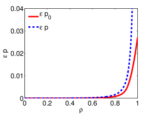
The choice of δ𝛿\delta makes sure that p0subscript𝑝0p_{0} and its derivatives up to second order are always bounded. To make sure all the coefficients appearing in the elliptic equation we will derive in the next section are continuous, we choose p0subscript𝑝0p_{0} to be a second order approximation to p𝑝p, instead of a first order one. For later usage, also note that the function p1(ρ)subscript𝑝1𝜌p_{1}(\rho) is invertible. This is easily seen from the property of function p𝑝p and p0subscript𝑝0p_{0}, see Fig 2.

Refer to caption
Figure 2: The plots of εp𝜀𝑝\varepsilon p and εp0𝜀subscript𝑝0\varepsilon p_{0} as functions of ρ𝜌\rho with ε=104,γ=2formulae-sequence𝜀superscript104𝛾2\varepsilon=10^{-4},\gamma=2.

By the definition, the Courant-Friedrich-Lewy (CFL) condition for the explicit part is

ΔtσΔxmax{|𝒒ρ|+εp0(ρ)},Δ𝑡𝜎Δ𝑥𝒒𝜌𝜀superscriptsubscript𝑝0𝜌\displaystyle\Delta t\leq\frac{\sigma\Delta x}{\max\{|\frac{\boldsymbol{q}}{\rho}|+\sqrt{\varepsilon p_{0}^{\prime}(\rho)}\}}, (18)

where σ𝜎\sigma is the Courant number. Since εp0𝜀superscriptsubscript𝑝0\varepsilon p_{0}^{\prime} is always bounded, the CFL condition can be satisfied uniformly in ε𝜀\varepsilon.

3.2 The Direct method

To get the solution, we will rewrite the above scheme into another form. By inserting (15) into (14), we can get an elliptic equation for ρ𝜌\rho:

ρn+1ρnΔt+𝒙𝒒nΔtΔ𝒙(εp1(ρn+1))Δt𝒙2:(𝒒n𝒒nρn)ΔtΔ𝒙(εp0(ρn))=0.:superscript𝜌𝑛1superscript𝜌𝑛Δ𝑡subscript𝒙superscript𝒒𝑛Δ𝑡subscriptΔ𝒙𝜀subscript𝑝1superscript𝜌𝑛1Δ𝑡superscriptsubscript𝒙2tensor-productsuperscript𝒒𝑛superscript𝒒𝑛superscript𝜌𝑛Δ𝑡subscriptΔ𝒙𝜀subscript𝑝0superscript𝜌𝑛0\displaystyle\begin{split}&\frac{\rho^{{n+1}}-\rho^{{n}}}{\Delta t}+\nabla_{\boldsymbol{x}}\cdot\boldsymbol{q}^{n}-\Delta t\Delta_{\boldsymbol{x}}(\varepsilon p_{1}(\rho^{{n+1}}))-\Delta t\nabla_{\boldsymbol{x}}^{2}:\left(\frac{\boldsymbol{q}^{n}\otimes\boldsymbol{q}^{n}}{\rho^{n}}\right)-\Delta t\Delta_{\boldsymbol{x}}\left(\varepsilon p_{0}(\rho^{{n}})\right)=0.\end{split} (19)

From this equation, we can solve ρn+1superscript𝜌𝑛1\rho^{n+1}. However, if we solve ρ𝜌\rho directly, the density constraint ρρ𝜌superscript𝜌\rho\leq\rho^{*} may not be satisfied due to discretization errors. Thus, we write ρn+1=ρ(p1n+1)superscript𝜌𝑛1𝜌superscriptsubscript𝑝1𝑛1\rho^{n+1}=\rho(p_{1}^{n+1}) in (19) and solve the equation in terms of p1subscript𝑝1p_{1}. The density constraint ρρ𝜌superscript𝜌\rho\leq\rho^{*} will be automatically satisfied. Moreover, the positivity of ρ𝜌\rho can be ensured by the fact that the discretized equation satisfies the maximal principle.

Once ρn+1superscript𝜌𝑛1\rho^{n+1} is obtained, we can obtain 𝒒n+1superscript𝒒𝑛1\boldsymbol{q}^{n+1} from (15) easily.

𝒒n+1=𝒒nΔt{𝒙(𝒒n𝒒nρn)+𝒙(εp0(ρn))+𝒙(εp1(ρn+1))}.superscript𝒒𝑛1superscript𝒒𝑛Δ𝑡subscript𝒙tensor-productsuperscript𝒒𝑛superscript𝒒𝑛superscript𝜌𝑛subscript𝒙𝜀subscript𝑝0superscript𝜌𝑛subscript𝒙𝜀subscript𝑝1superscript𝜌𝑛1\displaystyle\boldsymbol{q}^{n+1}=\boldsymbol{q}^{n}-{\Delta t}\left\{\nabla_{\boldsymbol{x}}\cdot\left(\frac{\boldsymbol{q}^{n}\otimes\boldsymbol{q}^{n}}{\rho^{n}}\right)+\nabla_{\boldsymbol{x}}\left(\varepsilon p_{0}(\rho^{n})\right)+\nabla_{\boldsymbol{x}}(\varepsilon p_{1}(\rho^{n+1}))\right\}. (20)
Remark 1

In the numerical simulation, we can also improve the accuracy by implementing a fully implicit scheme, which iterates the above scheme to solve (14) and (15) with 𝐪𝐪ρtensor-product𝐪𝐪𝜌\frac{\boldsymbol{q}\otimes\boldsymbol{q}}{\rho} implicit. Suppose ρn+1,0=ρnsuperscript𝜌𝑛10superscript𝜌𝑛\rho^{n+1,0}=\rho^{n} and 𝐪n+1,0=𝐪nsuperscript𝐪𝑛10superscript𝐪𝑛\boldsymbol{q}^{n+1,0}=\boldsymbol{q}^{n} and ρn+1,ksuperscript𝜌𝑛1𝑘\rho^{n+1,k}, 𝐪n+1,ksuperscript𝐪𝑛1𝑘\boldsymbol{q}^{n+1,k} are the solutions to the following equations.

ρn+1,k+1ρnΔt+𝒙𝒒nΔtΔ𝒙(εp1(ρn+1,k+1))superscript𝜌𝑛1𝑘1superscript𝜌𝑛Δ𝑡subscript𝒙superscript𝒒𝑛Δ𝑡subscriptΔ𝒙𝜀subscript𝑝1superscript𝜌𝑛1𝑘1\displaystyle\frac{\rho^{{n+1},k+1}-\rho^{{n}}}{\Delta t}+\nabla_{\boldsymbol{x}}\cdot\boldsymbol{q}^{n}-\Delta t\Delta_{\boldsymbol{x}}(\varepsilon p_{1}(\rho^{{n+1},k+1}))
Δt𝒙2:(𝒒n+1,k𝒒n+1,kρn+1,k)+Δ𝒙(εp0(ρn))=0,:Δ𝑡superscriptsubscript𝒙2tensor-productsuperscript𝒒𝑛1𝑘superscript𝒒𝑛1𝑘superscript𝜌𝑛1𝑘subscriptΔ𝒙𝜀subscript𝑝0superscript𝜌𝑛0\displaystyle\qquad\qquad\qquad-\Delta t\ \nabla_{\boldsymbol{x}}^{2}:\left(\frac{\boldsymbol{q}^{n+1,k}\otimes\boldsymbol{q}^{n+1,k}}{\rho^{n+1,k}}\right)+\Delta_{\boldsymbol{x}}\left(\varepsilon p_{0}(\rho^{{n}})\right)=0, (21)
𝒒n+1,k+1=𝒒nΔt{𝒙(𝒒n+1,k𝒒n+1,kρn+1,k)+𝒙(εp0(ρn))+𝒙(εp1(ρn+1,k+1))}.superscript𝒒𝑛1𝑘1superscript𝒒𝑛Δ𝑡subscript𝒙tensor-productsuperscript𝒒𝑛1𝑘superscript𝒒𝑛1𝑘superscript𝜌𝑛1𝑘subscript𝒙𝜀subscript𝑝0superscript𝜌𝑛subscript𝒙𝜀subscript𝑝1superscript𝜌𝑛1𝑘1\displaystyle\boldsymbol{q}^{n+1,k+1}=\boldsymbol{q}^{n}-{\Delta t}\left\{\nabla_{\boldsymbol{x}}\left(\frac{\boldsymbol{q}^{n+1,k}\otimes\boldsymbol{q}^{n+1,k}}{\rho^{n+1,k}}\right)+\nabla_{\boldsymbol{x}}\left(\varepsilon p_{0}(\rho^{n})\right)+\nabla_{\boldsymbol{x}}(\varepsilon p_{1}(\rho^{n+1,k+1}))\right\}. (22)

As k𝑘k\to\infty, the solution approximates to the one solving the fully implicit scheme (both in ρ𝜌\rho and 𝐪𝐪ρtensor-product𝐪𝐪𝜌\frac{\boldsymbol{q}\otimes\boldsymbol{q}}{\rho}). This modification provides little improvement compared to the additional computational cost.

3.3 The Gauge method

Another way to implement the AP scheme is the Gauge method developed in [16]. It can be obtained by applying the Gauge decomposition

𝒒=𝒂𝒙φ,𝒙𝒂=0formulae-sequence𝒒𝒂subscript𝒙𝜑subscript𝒙𝒂0\displaystyle\boldsymbol{q}=\boldsymbol{a}-\nabla_{\boldsymbol{x}}\varphi,\quad\nabla_{\boldsymbol{x}}\cdot\boldsymbol{a}=0 (23)

where 𝒂𝒂\boldsymbol{a} is the incompressible part of field 𝒒𝒒\boldsymbol{q} and φ𝜑\varphi is the irrotational one. This decomposition is expected to be more robust for capturing incompressibility constraint. We will see that it is partially right. By including this decomposition into equations (14) and (15), we get

ρn+1ρnΔt+𝒙𝒒nΔtΔ𝒙(εp1(ρn+1))Δt𝒙2:(𝒒n𝒒nρn)ΔtΔ𝒙(εp0(ρn))=0,:superscript𝜌𝑛1superscript𝜌𝑛Δ𝑡subscript𝒙superscript𝒒𝑛Δ𝑡subscriptΔ𝒙𝜀subscript𝑝1superscript𝜌𝑛1Δ𝑡superscriptsubscript𝒙2tensor-productsuperscript𝒒𝑛superscript𝒒𝑛superscript𝜌𝑛Δ𝑡subscriptΔ𝒙𝜀subscript𝑝0superscript𝜌𝑛0\displaystyle\begin{split}&\frac{\rho^{{n+1}}-\rho^{{n}}}{\Delta t}+\nabla_{\boldsymbol{x}}\cdot\boldsymbol{q}^{n}-\Delta t\Delta_{\boldsymbol{x}}(\varepsilon p_{1}(\rho^{{n+1}}))\\ &\hskip 85.35826pt-\Delta t\nabla_{\boldsymbol{x}}^{2}:\left(\frac{\boldsymbol{q}^{n}\otimes\boldsymbol{q}^{n}}{\rho^{n}}\right)-\Delta t\Delta_{\boldsymbol{x}}(\varepsilon p_{0}(\rho^{{n}}))=0,\end{split} (24)
Δ𝒙φn+1=1Δt(ρn+1ρn),subscriptΔ𝒙superscript𝜑𝑛11Δ𝑡superscript𝜌𝑛1superscript𝜌𝑛\displaystyle\Delta_{\boldsymbol{x}}\varphi^{n+1}=\frac{1}{\Delta t}(\rho^{n+1}-\rho^{n}), (25)
Δ𝒙Pn+1=𝒙2:(𝒒n𝒒nρn)Δ𝒙(εp0(ρn)),:subscriptΔ𝒙superscript𝑃𝑛1superscriptsubscript𝒙2tensor-productsuperscript𝒒𝑛superscript𝒒𝑛superscript𝜌𝑛subscriptΔ𝒙𝜀subscript𝑝0superscript𝜌𝑛\displaystyle\Delta_{\boldsymbol{x}}P^{n+1}=-\nabla_{\boldsymbol{x}}^{2}:\left(\frac{\boldsymbol{q}^{n}\otimes\boldsymbol{q}^{n}}{\rho^{n}}\right)-\Delta_{\boldsymbol{x}}(\varepsilon p_{0}(\rho^{n})), (26)
𝒂n+1𝒂nΔt+𝒙(𝒒n𝒒nρn)+𝒙(εp0(ρn))+𝒙Pn+1=0,superscript𝒂𝑛1superscript𝒂𝑛Δ𝑡subscript𝒙tensor-productsuperscript𝒒𝑛superscript𝒒𝑛superscript𝜌𝑛subscript𝒙𝜀subscript𝑝0superscript𝜌𝑛subscript𝒙superscript𝑃𝑛10\displaystyle\frac{\boldsymbol{a}^{n+1}-\boldsymbol{a}^{n}}{\Delta t}+\nabla_{\boldsymbol{x}}\cdot\left(\frac{\boldsymbol{q}^{n}\otimes\boldsymbol{q}^{n}}{\rho^{n}}\right)+\nabla_{\boldsymbol{x}}(\varepsilon p_{0}(\rho^{n}))+\nabla_{\boldsymbol{x}}P^{n+1}=0, (27)
𝒒n+1=𝒂n+1𝒙φn+1.superscript𝒒𝑛1superscript𝒂𝑛1subscript𝒙superscript𝜑𝑛1\displaystyle\boldsymbol{q}^{n+1}=\boldsymbol{a}^{n+1}-\nabla_{\boldsymbol{x}}\varphi^{n+1}. (28)

Indeed, the equation (24) for p1n+1superscriptsubscript𝑝1𝑛1p_{1}^{n+1} is derived from (14) and (15) similarly as in the Direct method. The Laplace equation (25) for φn+1superscript𝜑𝑛1\varphi^{n+1} is the direct consequence of applying the decomposition (28) and 𝒙𝒂n+1=0subscript𝒙superscript𝒂𝑛10\nabla_{\boldsymbol{x}}\cdot\boldsymbol{a}^{n+1}=0 to the density equation (14). The equation (26) for Pn+1superscript𝑃𝑛1P^{n+1} and the equation (27) for 𝒂n+1superscript𝒂𝑛1\boldsymbol{a}^{n+1} are obtained by inserting (28) and 𝒙𝒂n+1=𝒙𝒂n=0subscript𝒙superscript𝒂𝑛1subscript𝒙superscript𝒂𝑛0\nabla_{\boldsymbol{x}}\cdot\boldsymbol{a}^{n+1}=\nabla_{\boldsymbol{x}}\cdot\boldsymbol{a}^{n}=0 into the momentum equation (15). Here a new unknown P𝑃P is introduced, which is defined by

Pn+1=εp1(ρn+1)φn+1φnΔt,superscript𝑃𝑛1𝜀subscript𝑝1superscript𝜌𝑛1superscript𝜑𝑛1superscript𝜑𝑛Δ𝑡\displaystyle P^{n+1}=\varepsilon p_{1}(\rho^{n+1})-\frac{\varphi^{n+1}-\varphi^{n}}{\Delta t}, (29)

since (24)-(25) and (27) imply (15).

The original equations (14) and (15) can also be recovered from (24)-(28) by assuming 𝒙𝒂n=0subscript𝒙superscript𝒂𝑛0\nabla_{\boldsymbol{x}}\cdot\boldsymbol{a}^{n}=0. In fact, the equations for Pn+1superscript𝑃𝑛1P^{n+1} and 𝒂n+1superscript𝒂𝑛1\boldsymbol{a}^{n+1} ((26)-(27)) and 𝒙𝒂n=0subscript𝒙superscript𝒂𝑛0\nabla_{\boldsymbol{x}}\cdot\boldsymbol{a}^{n}=0 imply 𝒙𝒂n+1=0subscript𝒙superscript𝒂𝑛10\nabla_{\boldsymbol{x}}\cdot\boldsymbol{a}^{n+1}=0. This leads to the density equation (14) from the φn+1superscript𝜑𝑛1\varphi^{n+1} equation (25) and the decomposition (28). (14) combined with the p1n+1superscriptsubscript𝑝1𝑛1p_{1}^{n+1} equation (24) will then allow us to recover the momentum equation (15).

The boundary conditions

By solving the equations (24)-(28) in sequential order, we can update the value of ρ,𝒒𝜌𝒒\rho,\boldsymbol{q}. To do this, we need to provide boundary conditions for the Laplace equations for φ𝜑\varphi and P𝑃P. The boundary conditions for Pn+1superscript𝑃𝑛1P^{n+1} are somehow straightforward due to the implicit relation (29), once φ𝜑\varphi is known. And in solving φn+1superscript𝜑𝑛1\varphi^{n+1}, we may impose Dirichlet boundary condition on φn+1superscript𝜑𝑛1\varphi^{n+1} as follows:

φn+1|Ω=0.evaluated-atsuperscript𝜑𝑛1Ω0\displaystyle\varphi^{n+1}|_{\Omega}=0. (30)

Indeed, other non-homogeneous Dirichlet boundary conditions can be chosen. This makes the unknown φn+1superscript𝜑𝑛1\varphi^{n+1} determined up to a linear function in space. However, this uncertainty can be removed by redefining 𝒂n+1superscript𝒂𝑛1\boldsymbol{a}^{n+1}. So we can always impose the homogeneous Dirichlet boundary conditions.

Simplification in the one dimensional case

Observe that in the one dimensional case, 𝒙a=0subscript𝒙𝑎0\nabla_{\boldsymbol{x}}\cdot a=0 implies that a𝑎a is independent of x𝑥x. We may thus rewrite (26) and (27) into a simpler equation by using (29)

an+1=anΔtcb((qn)2ρn+εp0(ρn)+εp1(ρn+1))|bc+1cb(φn+1|bcφn|bc),superscript𝑎𝑛1superscript𝑎𝑛evaluated-atΔ𝑡𝑐𝑏superscriptsuperscript𝑞𝑛2superscript𝜌𝑛𝜀subscript𝑝0superscript𝜌𝑛𝜀subscript𝑝1superscript𝜌𝑛1𝑏𝑐1𝑐𝑏evaluated-atsuperscript𝜑𝑛1𝑏𝑐evaluated-atsuperscript𝜑𝑛𝑏𝑐\displaystyle a^{n+1}=a^{n}-\frac{\Delta t}{c-b}\left(\frac{(q^{n})^{2}}{\rho^{n}}+\varepsilon p_{0}(\rho^{n})+\varepsilon p_{1}(\rho^{n+1})\right)\bigg{|}^{c}_{b}+\frac{1}{c-b}\left(\varphi^{n+1}|^{c}_{b}-\varphi^{n}|^{c}_{b}\right), (31)

where the space-domain is [b,c]𝑏𝑐[b,c] and f|bc=f(c)f(b)evaluated-at𝑓𝑏𝑐𝑓𝑐𝑓𝑏f|^{c}_{b}=f(c)-f(b). This equation can be further simplified, since we impose the homogeneous Dirichlet boundary condition on φ𝜑\varphi all the time. This lead to

an+1=anΔtcb((qn)2ρn+εp0(ρn)+εp1(ρn+1))|bc.superscript𝑎𝑛1superscript𝑎𝑛evaluated-atΔ𝑡𝑐𝑏superscriptsuperscript𝑞𝑛2superscript𝜌𝑛𝜀subscript𝑝0superscript𝜌𝑛𝜀subscript𝑝1superscript𝜌𝑛1𝑏𝑐\displaystyle a^{n+1}=a^{n}-\frac{\Delta t}{c-b}\left(\frac{(q^{n})^{2}}{\rho^{n}}+\varepsilon p_{0}(\rho^{n})+\varepsilon p_{1}(\rho^{n+1})\right)\bigg{|}^{c}_{b}. (32)

With this reformulation, in the one dimensional case, we can reduce the number of elliptic equations to be solved to one and update the space independent variable a𝑎a more efficiently. Also as a consequence of (30), ansuperscript𝑎𝑛a^{n} should be defined as the average of qnsuperscript𝑞𝑛q^{n}.

an=1cbbcqn𝑑x.superscript𝑎𝑛1𝑐𝑏superscriptsubscript𝑏𝑐superscript𝑞𝑛differential-d𝑥\displaystyle a^{n}=\frac{1}{c-b}\int_{b}^{c}q^{n}dx. (33)

In summary, the Gauge method in the one dimensional case is implemented through equations (24), (25), (28) and (32).

3.4 Discussion of the AP property

As for the AP property of the scheme, we give a formal proof. To be precise, we want to show that the system (19) and (15) becomes the incompressible Euler system as ε0𝜀0\varepsilon\to 0 in the congested region.

However, in contrast with the low Mach number limit of the isentropic Euler equation discussed in [18] or [16], the singularity in our model is embedded in the definition of p𝑝p. New congestion regions may arise from non-congested ones. And by the analysis in section A, there is the possibility that ρερsuperscript𝜌𝜀superscript𝜌\rho^{\varepsilon}\to\rho^{*} but the limit of the pressure εp1(ρε)0𝜀subscript𝑝1superscript𝜌𝜀0\varepsilon p_{1}(\rho^{\varepsilon})\to 0 as ε0𝜀0\varepsilon\to 0. This means that although the congestion density is reached, there is no real congestion in this region. So it seems better to characterize the congestion region by defining p¯=limε0εp1(ρε)>0¯𝑝subscript𝜀0𝜀subscript𝑝1superscript𝜌𝜀0\bar{p}=\lim_{\varepsilon\to 0}\varepsilon p_{1}(\rho^{\varepsilon})>0.

Currently, we can only show that in regions where both p¯n+1=limε0εp1((ρn+1)ε)>0superscript¯𝑝𝑛1subscript𝜀0𝜀subscript𝑝1superscriptsuperscript𝜌𝑛1𝜀0\bar{p}^{n+1}=\lim_{\varepsilon\to 0}\varepsilon p_{1}((\rho^{n+1})^{\varepsilon})>0 and p¯n=limε0εp1((ρn)ε)>0superscript¯𝑝𝑛subscript𝜀0𝜀subscript𝑝1superscriptsuperscript𝜌𝑛𝜀0\bar{p}^{n}=\lim_{\varepsilon\to 0}\varepsilon p_{1}((\rho^{n})^{\varepsilon})>0, (19) and (20) tend to the incompressible Euler system as ε0𝜀0\varepsilon\to 0. The assumption p¯n+1=limε0εp1((ρn+1)ε)>0superscript¯𝑝𝑛1subscript𝜀0𝜀subscript𝑝1superscriptsuperscript𝜌𝑛1𝜀0\bar{p}^{n+1}=\lim_{\varepsilon\to 0}\varepsilon p_{1}((\rho^{n+1})^{\varepsilon})>0 is somehow essential given that declustering wave may appear in our model, since the pressure p¯¯𝑝\bar{p} can change from positive value to 00 instantaneously due to a declustering wave. The assumption p¯n=limε0εp1((ρn)ε)>0superscript¯𝑝𝑛subscript𝜀0𝜀subscript𝑝1superscriptsuperscript𝜌𝑛𝜀0\bar{p}^{n}=\lim_{\varepsilon\to 0}\varepsilon p_{1}((\rho^{n})^{\varepsilon})>0 is also needed in case of the appearance of new congestion regions. In regions where p¯n+1>0superscript¯𝑝𝑛10\bar{p}^{n+1}>0 and p¯n>0superscript¯𝑝𝑛0\bar{p}^{n}>0, we have naturally that (ρn+1)ερsuperscriptsuperscript𝜌𝑛1𝜀superscript𝜌(\rho^{n+1})^{\varepsilon}\to\rho^{*} and (ρn)ερsuperscriptsuperscript𝜌𝑛𝜀superscript𝜌(\rho^{n})^{\varepsilon}\to\rho^{*} as ε0𝜀0\varepsilon\to 0. Taking the divergence of (20) and using (19), we can indeed recover (14), which leads to the incompressibility of (𝒒n+1)εsuperscriptsuperscript𝒒𝑛1𝜀(\boldsymbol{q}^{n+1})^{\varepsilon}: 𝒙(𝒒n+1)n+1=0subscript𝒙superscriptsuperscript𝒒𝑛1𝑛10\nabla_{\boldsymbol{x}}\cdot(\boldsymbol{q}^{n+1})^{n+1}=0. Here the implicitness in (14) is crucial. Then (11) follows. Although we can only prove the AP property inside a congestion region, the numerical solutions provide evidence that the scheme is globally AP, including at transition between compressible and incompressible region.

As for the Gauge method, it is also AP since it is a direct consequence of (14) and (15).

In the numerical simulations, we will check the AP property for concrete test cases.

4 Full time and space discretization

In this section, we present the one dimensional full time and space discretization. The two dimensional discretization is the easy extension of the one dimensional case. For the sake of completeness, we include it in the appendix.

The Direct method:

In the following, we consider the domain [b,c]=[0,1]𝑏𝑐01[b,c]=[0,1]. Let the uniform spatial mesh be Δx=1MΔ𝑥1𝑀\Delta x=\frac{1}{M}, where M𝑀M is a positive integer. Denote by Ujn+1=(ρjn,qjn)Tsuperscriptsubscript𝑈𝑗𝑛1superscriptsuperscriptsubscript𝜌𝑗𝑛superscriptsubscript𝑞𝑗𝑛𝑇U_{j}^{n+1}=(\rho_{j}^{n},q_{j}^{n})^{T} the approximations of U=(ρ,q)T𝑈superscript𝜌𝑞𝑇U=(\rho,q)^{T} at time tn=nΔtsuperscript𝑡𝑛𝑛Δ𝑡t^{n}=n\Delta t and positions xj=jΔxsubscript𝑥𝑗𝑗Δ𝑥x_{j}=j\Delta x, for j=0,1,,M𝑗01𝑀j=0,1,\ldots,M. We fully discretize the scheme (14) and (15) in the spirit of a local Lax-Friedrichs (or Rusanov) method [27] as follows:

ρjn+1ρjnΔt+1Δx[Qj+1/2(Ujn,Uj+1n,Ujn+1,Uj+1n+1)Qj1/2(Uj1n,Ujn,Uj1n+1,Ujn+1)]=0,subscriptsuperscript𝜌𝑛1𝑗subscriptsuperscript𝜌𝑛𝑗Δ𝑡1Δ𝑥delimited-[]subscript𝑄𝑗12superscriptsubscript𝑈𝑗𝑛superscriptsubscript𝑈𝑗1𝑛superscriptsubscript𝑈𝑗𝑛1superscriptsubscript𝑈𝑗1𝑛1subscript𝑄𝑗12superscriptsubscript𝑈𝑗1𝑛superscriptsubscript𝑈𝑗𝑛superscriptsubscript𝑈𝑗1𝑛1superscriptsubscript𝑈𝑗𝑛10\displaystyle\begin{split}\frac{\rho^{n+1}_{j}-\rho^{n}_{j}}{\Delta t}+\frac{1}{\Delta x}\bigg{[}&Q_{j+1/2}(U_{j}^{n},U_{j+1}^{n},U_{j}^{n+1},U_{j+1}^{n+1})\\ &-Q_{j-1/2}(U_{j-1}^{n},U_{j}^{n},U_{j-1}^{n+1},U_{j}^{n+1})\bigg{]}=0,\end{split} (34)
qjn+1qjnΔt+1Δx[Fj+1/2(Ujn,Uj+1n)Fj1/2(Uj1n,Ujn)]+12Δx[εp1(ρj+1n+1)εp1(ρj1n+1)]=0.subscriptsuperscript𝑞𝑛1𝑗subscriptsuperscript𝑞𝑛𝑗Δ𝑡1Δ𝑥delimited-[]subscript𝐹𝑗12superscriptsubscript𝑈𝑗𝑛superscriptsubscript𝑈𝑗1𝑛subscript𝐹𝑗12superscriptsubscript𝑈𝑗1𝑛superscriptsubscript𝑈𝑗𝑛12Δ𝑥delimited-[]𝜀subscript𝑝1superscriptsubscript𝜌𝑗1𝑛1𝜀subscript𝑝1superscriptsubscript𝜌𝑗1𝑛10\displaystyle\begin{split}\frac{q^{n+1}_{j}-q^{n}_{j}}{\Delta t}&+\frac{1}{\Delta x}\left[F_{j+1/2}(U_{j}^{n},U_{j+1}^{n})-F_{j-1/2}(U_{j-1}^{n},U_{j}^{n})\right]\\ &+\frac{1}{2\Delta x}\left[\varepsilon p_{1}(\rho_{j+1}^{n+1})-\varepsilon p_{1}(\rho_{j-1}^{n+1})\right]=0.\end{split} (35)

where the fluxes are given by:

Qj+1/2n+1/2=12[qjn+1+qj+1n+1]12Cj+1/2n(ρj+1nρjn),superscriptsubscript𝑄𝑗12𝑛1212delimited-[]superscriptsubscript𝑞𝑗𝑛1superscriptsubscript𝑞𝑗1𝑛112superscriptsubscript𝐶𝑗12𝑛superscriptsubscript𝜌𝑗1𝑛superscriptsubscript𝜌𝑗𝑛\displaystyle Q_{j+1/2}^{n+1/2}=\frac{1}{2}\left[q_{j}^{n+1}+q_{j+1}^{n+1}\right]-\frac{1}{2}C_{j+1/2}^{n}(\rho_{j+1}^{n}-\rho_{j}^{n}), (36)
Fj+1/2n=12[(qjn)2ρjn+(qj+1n)2ρj+1n+εp0(ρj+1n)+εp0(ρjn)]12Cj+1/2n(qj+1nqjn).superscriptsubscript𝐹𝑗12𝑛12delimited-[]superscriptsuperscriptsubscript𝑞𝑗𝑛2superscriptsubscript𝜌𝑗𝑛superscriptsuperscriptsubscript𝑞𝑗1𝑛2superscriptsubscript𝜌𝑗1𝑛𝜀subscript𝑝0superscriptsubscript𝜌𝑗1𝑛𝜀subscript𝑝0superscriptsubscript𝜌𝑗𝑛12superscriptsubscript𝐶𝑗12𝑛superscriptsubscript𝑞𝑗1𝑛superscriptsubscript𝑞𝑗𝑛\displaystyle F_{j+1/2}^{n}=\frac{1}{2}\left[\frac{(q_{j}^{n})^{2}}{\rho_{j}^{n}}+\frac{(q_{j+1}^{n})^{2}}{\rho_{j+1}^{n}}+\varepsilon p_{0}(\rho_{j+1}^{n})+\varepsilon p_{0}(\rho_{j}^{n})\right]-\frac{1}{2}C_{j+1/2}^{n}(q_{j+1}^{n}-q_{j}^{n}). (37)

They consist of the sum of a centered flux, implicit in (36) , explicit in (37) and biased terms introducing diffusion. The quantity Cj+1/2nsuperscriptsubscript𝐶𝑗12𝑛C_{j+1/2}^{n} is the local diffusion coefficient and is given by:

Cj+1/2n=max{|qjnρjn|+εp0(ρjn),|qj+1nρj+1n|+εp0(ρj+1n)}.superscriptsubscript𝐶𝑗12𝑛superscriptsubscript𝑞𝑗𝑛superscriptsubscript𝜌𝑗𝑛𝜀superscriptsubscript𝑝0superscriptsubscript𝜌𝑗𝑛superscriptsubscript𝑞𝑗1𝑛superscriptsubscript𝜌𝑗1𝑛𝜀superscriptsubscript𝑝0superscriptsubscript𝜌𝑗1𝑛\displaystyle C_{j+1/2}^{n}=\max\left\{\left|\frac{q_{j}^{n}}{\rho_{j}^{n}}\right|+\sqrt{\varepsilon p_{0}^{\prime}(\rho_{j}^{n})},\left|\frac{q_{j+1}^{n}}{\rho_{j+1}^{n}}\right|+\sqrt{\varepsilon p_{0}^{\prime}(\rho_{j+1}^{n})}\right\}. (38)

It is defined as the local maximal characteristic speed related to the explicit pressure p0subscript𝑝0p_{0}. Therefore, it remains bounded as ε𝜀\varepsilon goes to zero. The quantity Cj+1/2nsuperscriptsubscript𝐶𝑗12𝑛C_{j+1/2}^{n} provides a numerical viscosity which is needed for scheme stability. We note that only the central discretization part of the flux is taken implicit, while the numerical viscosity part is kept explicit. In the momentum flux, only the part of the flux which relates to pressure is taken implicit.

Based on this discretization, we can apply the same strategy as described in section 3.2 to get an elliptic equation in ρ𝜌\rho by substituting (35) into (34):

ρjn+1ρjnΔt+qj+1nqj1n2ΔxΔt4Δx2[εp1(ρj+2n+1)2εp1(ρjn+1)+εp1(ρj2n+1)]12Δx[Cj+1/2(ρj+1nρjn)Cj1/2(ρjnρj1n)]Δt2Δx2[Fj+3/2nFj+1/2nFj1/2n+Fj3/2n]=0.subscriptsuperscript𝜌𝑛1𝑗subscriptsuperscript𝜌𝑛𝑗Δ𝑡superscriptsubscript𝑞𝑗1𝑛superscriptsubscript𝑞𝑗1𝑛2Δ𝑥Δ𝑡4Δsuperscript𝑥2delimited-[]𝜀subscript𝑝1superscriptsubscript𝜌𝑗2𝑛12𝜀subscript𝑝1superscriptsubscript𝜌𝑗𝑛1𝜀subscript𝑝1superscriptsubscript𝜌𝑗2𝑛112Δ𝑥delimited-[]subscript𝐶𝑗12superscriptsubscript𝜌𝑗1𝑛superscriptsubscript𝜌𝑗𝑛subscript𝐶𝑗12superscriptsubscript𝜌𝑗𝑛superscriptsubscript𝜌𝑗1𝑛Δ𝑡2Δsuperscript𝑥2delimited-[]superscriptsubscript𝐹𝑗32𝑛superscriptsubscript𝐹𝑗12𝑛superscriptsubscript𝐹𝑗12𝑛superscriptsubscript𝐹𝑗32𝑛0\displaystyle\begin{split}\frac{\rho^{n+1}_{j}-\rho^{n}_{j}}{\Delta t}&+\frac{q_{j+1}^{n}-q_{j-1}^{n}}{2\Delta x}-\frac{\Delta t}{4\Delta x^{2}}\left[\varepsilon p_{1}(\rho_{j+2}^{n+1})-2\varepsilon p_{1}(\rho_{j}^{n+1})+\varepsilon p_{1}(\rho_{j-2}^{n+1})\right]\\ &-\frac{1}{2\Delta x}\left[C_{j+1/2}(\rho_{j+1}^{n}-\rho_{j}^{n})-C_{j-1/2}(\rho_{j}^{n}-\rho_{j-1}^{n})\right]\\ &-\frac{\Delta t}{2\Delta x^{2}}\left[F_{j+3/2}^{n}-F_{j+1/2}^{n}-F_{j-1/2}^{n}+F_{j-3/2}^{n}\right]=0.\end{split} (39)

This equation is consistent with equation (19) of the Direct method. Then we get a nonlinear equation for p1subscript𝑝1p_{1}:

ρ((p1)jn+1)Δt24Δx2[ε(p1)j+2n+12ε(p1)jn+1+ε(p1)j2n+1]=ρjnΔt2Δx(qj+1nqj1n)+Δt2Δx[Cj+1/2(ρj+1nρjn)Cj1/2(ρjnρj1n)]+Δt22Δx2[Fj+3/2nFj+1/2nFj1/2n+Fj3/2n].𝜌subscriptsuperscriptsubscript𝑝1𝑛1𝑗Δsuperscript𝑡24Δsuperscript𝑥2delimited-[]𝜀superscriptsubscriptsubscript𝑝1𝑗2𝑛12𝜀superscriptsubscriptsubscript𝑝1𝑗𝑛1𝜀superscriptsubscriptsubscript𝑝1𝑗2𝑛1subscriptsuperscript𝜌𝑛𝑗Δ𝑡2Δ𝑥superscriptsubscript𝑞𝑗1𝑛superscriptsubscript𝑞𝑗1𝑛Δ𝑡2Δ𝑥delimited-[]subscript𝐶𝑗12superscriptsubscript𝜌𝑗1𝑛superscriptsubscript𝜌𝑗𝑛subscript𝐶𝑗12superscriptsubscript𝜌𝑗𝑛superscriptsubscript𝜌𝑗1𝑛Δsuperscript𝑡22Δsuperscript𝑥2delimited-[]superscriptsubscript𝐹𝑗32𝑛superscriptsubscript𝐹𝑗12𝑛superscriptsubscript𝐹𝑗12𝑛superscriptsubscript𝐹𝑗32𝑛\displaystyle\begin{split}\rho((p_{1})^{n+1}_{j})&-\frac{\Delta t^{2}}{4\Delta x^{2}}\left[\varepsilon(p_{1})_{j+2}^{n+1}-2\varepsilon(p_{1})_{j}^{n+1}+\varepsilon(p_{1})_{j-2}^{n+1}\right]\\ =\ \rho^{n}_{j}&-\frac{\Delta t}{2\Delta x}(q_{j+1}^{n}-q_{j-1}^{n})+\frac{\Delta t}{2\Delta x}\left[C_{j+1/2}(\rho_{j+1}^{n}-\rho_{j}^{n})-C_{j-1/2}(\rho_{j}^{n}-\rho_{j-1}^{n})\right]\\ &+\frac{\Delta t^{2}}{2\Delta x^{2}}\left[F_{j+3/2}^{n}-F_{j+1/2}^{n}-F_{j-1/2}^{n}+F_{j-3/2}^{n}\right].\end{split} (40)

As mentioned before, we will use Newton iterations to solve this nonlinear equation and get p1n+1superscriptsubscript𝑝1𝑛1p_{1}^{n+1}. The density ρn+1superscript𝜌𝑛1\rho^{n+1} is then obtained by inverting the nonlinear function p1=p1(ρ)subscript𝑝1subscript𝑝1𝜌p_{1}=p_{1}(\rho) with another Newton iteration. Once ρn+1superscript𝜌𝑛1\rho^{n+1} is solved, qn+1superscript𝑞𝑛1q^{n+1} can be obtained by

qjn+1=Φ(Uj1n,Ujn,Uj+1n)Δt2Δx[εp1(ρj+1n+1)εp1(ρj1n+1)],subscriptsuperscript𝑞𝑛1𝑗Φsuperscriptsubscript𝑈𝑗1𝑛superscriptsubscript𝑈𝑗𝑛superscriptsubscript𝑈𝑗1𝑛Δ𝑡2Δ𝑥delimited-[]𝜀subscript𝑝1superscriptsubscript𝜌𝑗1𝑛1𝜀subscript𝑝1superscriptsubscript𝜌𝑗1𝑛1q^{n+1}_{j}=\Phi(U_{j-1}^{n},U_{j}^{n},U_{j+1}^{n})-\frac{\Delta t}{2\Delta x}\left[\varepsilon p_{1}(\rho_{j+1}^{n+1})-\varepsilon p_{1}(\rho_{j-1}^{n+1})\right], (41)

with

Φ(Uj1n,Ujn,Uj+1n)=qjnΔtΔx[Fj+1/2nFj1/2n].Φsuperscriptsubscript𝑈𝑗1𝑛superscriptsubscript𝑈𝑗𝑛superscriptsubscript𝑈𝑗1𝑛subscriptsuperscript𝑞𝑛𝑗Δ𝑡Δ𝑥delimited-[]superscriptsubscript𝐹𝑗12𝑛superscriptsubscript𝐹𝑗12𝑛\Phi(U_{j-1}^{n},U_{j}^{n},U_{j+1}^{n})=q^{n}_{j}-\frac{\Delta t}{\Delta x}\left[F_{j+1/2}^{n}-F_{j-1/2}^{n}\right]. (42)
The Gauge method

Also based on (34) and (35), we can have the full time-space discretization of the Gauge method. Indeed, for the Gauge method, we need to discretize (40). This leads to

14Δx2[φj+2n+12φjn+1+φj2n+1]=14Δsuperscript𝑥2delimited-[]subscriptsuperscript𝜑𝑛1𝑗22subscriptsuperscript𝜑𝑛1𝑗subscriptsuperscript𝜑𝑛1𝑗2absent\displaystyle\frac{1}{4\Delta x^{2}}\left[\varphi^{n+1}_{j+2}-2\varphi^{n+1}_{j}+\varphi^{n+1}_{j-2}\right]=
1Δt(ρjn+1ρjn)12Δx[Cj+1/2(ρj+1nρjn)Cj1/2(ρjnρj1n)],1Δ𝑡subscriptsuperscript𝜌𝑛1𝑗subscriptsuperscript𝜌𝑛𝑗12Δ𝑥delimited-[]subscript𝐶𝑗12superscriptsubscript𝜌𝑗1𝑛superscriptsubscript𝜌𝑗𝑛subscript𝐶𝑗12superscriptsubscript𝜌𝑗𝑛superscriptsubscript𝜌𝑗1𝑛\displaystyle\quad\quad\quad\frac{1}{\Delta t}(\rho^{n+1}_{j}-\rho^{n}_{j})-\frac{1}{2\Delta x}\left[C_{j+1/2}(\rho_{j+1}^{n}-\rho_{j}^{n})-C_{j-1/2}(\rho_{j}^{n}-\rho_{j-1}^{n})\right], (43)
an+1=anΔt((qnqn)ρn+εp0(ρn)+εp1(ρn+1))|01superscript𝑎𝑛1superscript𝑎𝑛evaluated-atΔ𝑡tensor-productsuperscript𝑞𝑛superscript𝑞𝑛superscript𝜌𝑛𝜀subscript𝑝0superscript𝜌𝑛𝜀subscript𝑝1superscript𝜌𝑛101\displaystyle a^{n+1}=a^{n}-{\Delta t}\left(\frac{(q^{n}\otimes q^{n})}{\rho^{n}}+\varepsilon p_{0}(\rho^{n})+\varepsilon p_{1}(\rho^{n+1})\right)\bigg{|}^{1}_{0}
+Δt21M[Cj+1/2(qj+1nqjn)Cj1/2(qjnqj1n)],Δ𝑡2superscriptsubscript1𝑀delimited-[]subscript𝐶𝑗12superscriptsubscript𝑞𝑗1𝑛superscriptsubscript𝑞𝑗𝑛subscript𝐶𝑗12superscriptsubscript𝑞𝑗𝑛superscriptsubscript𝑞𝑗1𝑛\displaystyle\quad\quad\quad+\frac{\Delta t}{2}\sum_{1}^{M}\left[C_{j+1/2}(q_{j+1}^{n}-q_{j}^{n})-C_{j-1/2}(q_{j}^{n}-q_{j-1}^{n})\right], (44)
qjn+1=an+112Δx(φj+1n+1φj1n+1).subscriptsuperscript𝑞𝑛1𝑗superscript𝑎𝑛112Δ𝑥subscriptsuperscript𝜑𝑛1𝑗1subscriptsuperscript𝜑𝑛1𝑗1\displaystyle q^{n+1}_{j}=a^{n+1}-\frac{1}{2\Delta x}(\varphi^{n+1}_{j+1}-\varphi^{n+1}_{j-1}). (45)

The above equations are the direct consequences of (24)-(25), (28) and (32). However, in the numerical simulation, we will mainly test the schemes with (43) replaced by

1Δx2[φj+1n+12φjn+1+φj1n+1]=1Δt(ρjn+1ρjn)12Δx[Cj+1/2(ρj+1nρjn)Cj1/2(ρjnρj1n)],1Δsuperscript𝑥2delimited-[]subscriptsuperscript𝜑𝑛1𝑗12subscriptsuperscript𝜑𝑛1𝑗subscriptsuperscript𝜑𝑛1𝑗11Δ𝑡subscriptsuperscript𝜌𝑛1𝑗subscriptsuperscript𝜌𝑛𝑗12Δ𝑥delimited-[]subscript𝐶𝑗12superscriptsubscript𝜌𝑗1𝑛superscriptsubscript𝜌𝑗𝑛subscript𝐶𝑗12superscriptsubscript𝜌𝑗𝑛superscriptsubscript𝜌𝑗1𝑛\displaystyle\begin{split}\frac{1}{\Delta x^{2}}\left[\varphi^{n+1}_{j+1}-2\varphi^{n+1}_{j}+\varphi^{n+1}_{j-1}\right]=&\ \frac{1}{\Delta t}(\rho^{n+1}_{j}-\rho^{n}_{j})\\ &-\frac{1}{2\Delta x}\left[C_{j+1/2}(\rho_{j+1}^{n}-\rho_{j}^{n})-C_{j-1/2}(\rho_{j}^{n}-\rho_{j-1}^{n})\right],\end{split} (46)

which may be justified as being the direct discretization of (25) with some numerical viscosity added to the right hand side. The stencils are different in two cases. We call the Gauge method with stencil (43) Gauge 2 method and the one with stencil (46) Gauge 1 method, since they use grids φj±2subscript𝜑plus-or-minus𝑗2\varphi_{j\pm 2} and φj±1subscript𝜑plus-or-minus𝑗1\varphi_{j\pm 1} respectively in addition to φjsubscript𝜑𝑗\varphi_{j}. There is a big difference in performance between the two discretizations. In fact, we will see in the next section that the Gauge 2 method ( with (43)) yields almost the same numerical result as the Direct method, while the Gauge 1 method (with (46)) performs quite differently from the Direct method. This may be partially due to the fact that the Gauge 1 method introduces more diffusion than the Gauge 2 method, which can be seen by inserting the Taylor expansion of φj±1n+1,φj±2n+1superscriptsubscript𝜑plus-or-minus𝑗1𝑛1superscriptsubscript𝜑plus-or-minus𝑗2𝑛1\varphi_{j\pm 1}^{n+1},\varphi_{j\pm 2}^{n+1} around x=jΔx𝑥𝑗Δ𝑥x=j\Delta x into the discretizations:

(1Δx2[φj+1n+12φjn+1+φj1n+1])(14Δx2[φj+2n+12φjn+1+φj2n+1])=14d4dx4φn+1(jΔx)Δx2+O(Δx4).\displaystyle\begin{split}&\left(-\frac{1}{\Delta x^{2}}\left[\varphi^{n+1}_{j+1}-2\varphi^{n+1}_{j}+\varphi^{n+1}_{j-1}\right]\right)-\left(-\frac{1}{4\Delta x^{2}}\left[\varphi^{n+1}_{j+2}-2\varphi^{n+1}_{j}+\varphi^{n+1}_{j-2}\right]\right)\\ &\quad\quad=\frac{1}{4}\frac{d^{4}}{dx^{4}}\varphi^{n+1}(j\Delta x)\Delta x^{2}+O(\Delta x^{4}).\end{split}
Numerical diffusion

An important issue about the scheme is the numerical diffusion. From the equation (40), it can be seen that the diffusion for ρ𝜌\rho is of the order of

(12(|un|+εp0(ρn))Δx+Δtεp1(ρn))Δ𝒙ρn+ΔtΔ𝒙(ρnunun).12superscript𝑢𝑛𝜀superscriptsubscript𝑝0superscript𝜌𝑛Δ𝑥Δ𝑡𝜀superscriptsubscript𝑝1superscript𝜌𝑛subscriptΔ𝒙superscript𝜌𝑛Δ𝑡subscriptΔ𝒙tensor-productsuperscript𝜌𝑛superscript𝑢𝑛superscript𝑢𝑛\displaystyle\left(\frac{1}{2}(|u^{n}|+\sqrt{\varepsilon p_{0}^{\prime}(\rho^{n})})\Delta x+\Delta t\varepsilon p_{1}^{\prime}(\rho^{n})\right)\Delta_{\boldsymbol{x}}\rho^{n}+\Delta t\Delta_{\boldsymbol{x}}(\rho^{n}u^{n}\otimes u^{n}). (47)

And similarly, by inserting (34) into the pressure p1subscript𝑝1p_{1} term in (35) we can see that the diffusion for q𝑞q is of the order of

(12(|un|+εp0(ρn)))ΔxΔxqn+Δtεp1(ρn)Δxqn.12superscript𝑢𝑛𝜀superscriptsubscript𝑝0superscript𝜌𝑛Δ𝑥subscriptΔ𝑥superscript𝑞𝑛Δ𝑡𝜀superscriptsubscript𝑝1superscript𝜌𝑛subscriptΔ𝑥superscript𝑞𝑛\displaystyle\left(\frac{1}{2}(|u^{n}|+\sqrt{\varepsilon p_{0}^{\prime}(\rho^{n})})\right)\Delta x\Delta_{{x}}{q}^{n}+\Delta t\varepsilon p_{1}^{\prime}(\rho^{n})\Delta_{{x}}{q}^{n}. (48)

To damp out the oscillations in the mass and momentum equations, the required numerical diffusion is [27]

(12(|un|+εp(ρn)))ΔxΔxρn,(12(|un|+εp(ρn)))ΔxΔxqn,12superscript𝑢𝑛𝜀superscript𝑝superscript𝜌𝑛Δ𝑥subscriptΔ𝑥superscript𝜌𝑛12superscript𝑢𝑛𝜀superscript𝑝superscript𝜌𝑛Δ𝑥subscriptΔ𝑥superscript𝑞𝑛\displaystyle\left(\frac{1}{2}(|u^{n}|+\sqrt{\varepsilon p^{\prime}(\rho^{n})})\right)\Delta x\Delta_{{x}}\rho^{n},\left(\frac{1}{2}(|u^{n}|+\sqrt{\varepsilon p^{\prime}(\rho^{n})})\right)\Delta x\Delta_{{x}}{q}^{n}, (49)

respectively. To ensure that this numerical diffusion is achieved, we need the condition

(12(|un|+εp0(ρn))Δx+εp1(ρn)Δt)(12(|un|+εp(ρn)))Δx,12superscript𝑢𝑛𝜀superscriptsubscript𝑝0superscript𝜌𝑛Δ𝑥𝜀superscriptsubscript𝑝1superscript𝜌𝑛Δ𝑡12superscript𝑢𝑛𝜀superscript𝑝superscript𝜌𝑛Δ𝑥\displaystyle\left(\frac{1}{2}(|u^{n}|+\sqrt{\varepsilon p_{0}^{\prime}(\rho^{n})})\Delta x+\varepsilon p_{1}^{\prime}(\rho^{n})\Delta t\right)\geq\left(\frac{1}{2}(|u^{n}|+\sqrt{\varepsilon p^{\prime}(\rho^{n})})\right)\Delta x, (50)

which leads to

ΔtΔx12(εp0(ρn)+εp(ρn)).Δ𝑡Δ𝑥12𝜀superscriptsubscript𝑝0superscript𝜌𝑛𝜀superscript𝑝superscript𝜌𝑛\displaystyle\frac{\Delta t}{\Delta x}\geq\frac{1}{2\left(\sqrt{\varepsilon p_{0}^{\prime}(\rho^{n})}+\sqrt{\varepsilon p^{\prime}(\rho^{n})}\right)}. (51)

This condition is automatically satisfied in the congested region (ρρ𝜌superscript𝜌\rho\to\rho^{*}) for small ε𝜀\varepsilon, since εp(ρn)𝜀superscript𝑝superscript𝜌𝑛\varepsilon p^{\prime}(\rho^{n})\to\infty as ε0𝜀0\varepsilon\to 0. However, it contradicts the CFL condition in the non-congested region for small ε𝜀\varepsilon, since εp(ρn)𝜀superscript𝑝superscript𝜌𝑛\varepsilon p^{\prime}(\rho^{n}) and εp0(ρn)0𝜀superscriptsubscript𝑝0superscript𝜌𝑛0\varepsilon p_{0}^{\prime}(\rho^{n})\to 0 as ε0𝜀0\varepsilon\to 0. From this analysis, there should be no oscillations in the congestion region while the numerical diffusion may not be sufficient in the non-congested region. However, numerical simulation seems to indicate that the numerical viscosity in this scheme is sufficient to damp out the oscillations in the non-congested region.

5 Numerical results

5.1 One dimensional test cases

In this section, we use several numerical examples to test the performance of the schemes. Corresponding to different situations, four examples are tested. All these examples are the compositions of Riemann problems. Since the exact solutions to Riemann problem can be determined as in section 2, we can compare the exact and numerical solutions. Different measurements of the relative errors will be applied to test the performance of our schemes. And the numerical Courant number is computed.

In the following, we choose γ=2𝛾2\gamma=2 and the maximal density ρ=1superscript𝜌1\rho^{*}=1. The test problems are:

(P1):(ρ,q)(x,0)={(0.7,0.8),x[0,0.5),(0.7,0.8),x(0.5,1],:𝑃1𝜌𝑞𝑥0cases0.70.8𝑥00.50.70.8𝑥0.51\displaystyle(P1):(\rho,q)(x,0)=\begin{cases}(0.7,0.8),&x\in[0,0.5),\\ (0.7,-0.8),&x\in(0.5,1],\end{cases} (52)
(P2):(ρ,q)(x,0)={(0.7,0.8),x[0,0.5),(0.7,0.8),x(0.5,1],:𝑃2𝜌𝑞𝑥0cases0.70.8𝑥00.50.70.8𝑥0.51\displaystyle(P2):(\rho,q)(x,0)=\begin{cases}(0.7,-0.8),&x\in[0,0.5),\\ (0.7,0.8),&x\in(0.5,1],\end{cases} (53)
(P3):(ρ,q)(x,0)={(0.7,0.8),x[0,0.25),(0.8,0.3),x(0.25,0.75),(0.7,1.2),x(0.75,1],:𝑃3𝜌𝑞𝑥0cases0.70.8𝑥00.250.80.3𝑥0.250.750.71.2𝑥0.751\displaystyle(P3):(\rho,q)(x,0)=\begin{cases}(0.7,0.8),&x\in[0,0.25),\\ (0.8,-0.3),&x\in(0.25,0.75),\\ (0.7,-1.2),&x\in(0.75,1],\end{cases} (54)
(P4):(ρ,q)(x,0)={(0.8,0.3),x[0,0.5),(0.5,0.1),x(0.5,1],:𝑃4𝜌𝑞𝑥0cases0.80.3𝑥00.50.50.1𝑥0.51\displaystyle(P4):(\rho,q)(x,0)=\begin{cases}(0.8,0.3),&x\in[0,0.5),\\ (0.5,0.1),&x\in(0.5,1],\end{cases} (55)

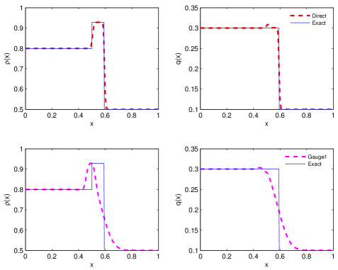
The first example (P1)𝑃1(P1) illustrates how the AP schemes capture shocks near congestion. The second example (P2)𝑃2(P2) shows how the AP schemes work near vacuum. The third example (P3)𝑃3(P3) simulates the interaction of two shocks near congestion. The last example (P4)𝑃4(P4) shows some problems in the Gauge 1 method and will be used to justify the splitting of p𝑝p.

Example 1. The solution to the Riemann problem (P1)𝑃1(P1) consists of two shocks propagating in the opposite directions. The density of the intermediate state is close to the maximal density. In the following, we will test the two methods described in section 4 with different parameters ε𝜀\varepsilon and different mesh sizes Δx,ΔtΔ𝑥Δ𝑡\Delta x,\Delta t.

  1. 1.

    First, we choose ε=104,Δx=5×10³,Δt=5×10⁴formulae-sequence𝜀superscript104formulae-sequenceΔ𝑥5superscript103Δ𝑡5superscript104\varepsilon=10^{-4},\Delta x=5\times 10^{-3},\Delta t=5\times 10^{-4}. We will compare the performances of the two methods proposed in section 4.
    Refer to caption
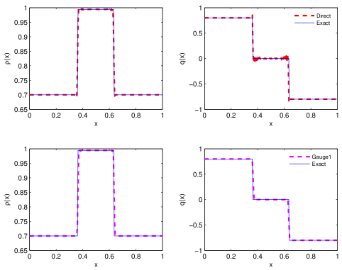
    Figure 3: The direct and Gauge 1 methods for problem (P1) at t=0.05𝑡0.05t=0.05 with ε=104,Δx=5×10³,Δt=5×10⁴formulae-sequence𝜀superscript104formulae-sequenceΔ𝑥5superscript103Δ𝑡5superscript104\varepsilon=10^{-4},\Delta x=5\times 10^{-3},\Delta t=5\times 10^{-4}. The solid lines are the exact solutions. The dashed curves are the numerical solutions. The left graphs are for ρ𝜌\rho, the right ones for q𝑞q, both as functions of x𝑥x.

    It can be seen from Figure 3 that there is large oscillations of the momentum in the congested region. But the propagation of the shock is captured well. In comparison, the Gauge 1 method as illustrated in Figure 3 eliminates all the oscillation.

  2. 2.

    We look how the choices of the parameters ε𝜀\varepsilon ΔxΔ𝑥\Delta x and ΔtΔ𝑡\Delta t affect the numerical result. We may fix Δx,ΔtΔ𝑥Δ𝑡\Delta x,\Delta t but change the value of ε𝜀\varepsilon so as to test the cases ε<Δt𝜀Δ𝑡\varepsilon<\Delta t and ε>Δt𝜀Δ𝑡\varepsilon>\Delta t.

    Refer to caption
    (a) ε=102𝜀superscript102\varepsilon=10^{-2}
    Refer to caption
    (b) ε=108𝜀superscript108\varepsilon=10^{-8}
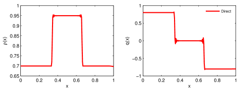
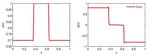
    Figure 4: Fix Δx=5×10³,Δt=5×10⁴formulae-sequenceΔ𝑥5superscript103Δ𝑡5superscript104\Delta x=5\times 10^{-3},\Delta t=5\times 10^{-4}. The numerical results of the Direct method for problem (P1) at t=0.05𝑡0.05t=0.05 with ε=102𝜀superscript102\varepsilon=10^{-2} and ε=108𝜀superscript108\varepsilon=10^{-8}. The left graphs are for ρ𝜌\rho, the right ones for q𝑞q, both as functions of x𝑥x.

    From the numerical results, it can be seen that the oscillations in the momentum always appear for different choices of ε𝜀\varepsilon but are smaller as ε0𝜀0\varepsilon\to 0 for this choice of parameter. This verifies the AP property. As for the Gauge 1 method, it has the same performance for all value of ε𝜀\varepsilon. Thus it shares the same property.

  3. 3.

    The above observation can be quantitatively investigated by measuring the difference between the numerical solution W𝑊W and the theoretical one w𝑤w. We use two measurements: one is the relative error of the numerical solution W𝑊W compared with w𝑤w in the sense of L1superscript𝐿1L^{1} norm and the other is the difference of their total variation:

    e(W)=WwL1wL1, where wL1=1Mj|wj|,formulae-sequence𝑒𝑊subscriptdelimited-∥∥𝑊𝑤superscript𝐿1subscriptdelimited-∥∥𝑤superscript𝐿1 where subscriptdelimited-∥∥𝑤superscript𝐿11𝑀subscript𝑗subscript𝑤𝑗\displaystyle e(W)=\frac{\lVert W-w\rVert_{L^{1}}}{\lVert w\rVert_{L^{1}}},\text{ where }\lVert w\rVert_{L^{1}}=\frac{1}{M}\sum_{j}\lvert w_{j}\rvert, (56)
    g(W)=|Tot.Var.{W}Tot.Var.{w}|Tot.Var.{w}, where Tot.Var.{w}=j|wj+1wj|.\displaystyle g(W)=\frac{\lvert\operatorname{Tot.Var.}\{W\}-\operatorname{Tot.Var.}\{w\}\rvert}{\operatorname{Tot.Var.}\{w\}},\text{ where }\operatorname{Tot.Var.}\{w\}=\sum_{j}\lvert w_{j+1}-w_{j}\rvert. (57)
    Parameters Direct Gauge 1
    ε𝜀\varepsilon ΔxΔ𝑥\Delta x ΔtΔ𝑡\Delta t e(W)𝑒𝑊e(W) ratio e(W)𝑒𝑊e(W) ratio
    104superscript10410^{-4} 1/20012001/200 1/25012501/250 1.1012×1021.1012superscript1021.1012\times 10^{-2} - 1.1209×1021.1209superscript1021.1209\times 10^{-2} -
    1/20012001/200 1/50015001/500 8.0103×1038.0103superscript1038.0103\times 10^{-3} 1.3747 7.8670×1037.8670superscript1037.8670\times 10^{-3} 1.4248
    1/20012001/200 1/1000110001/1000 4.2631×1034.2631superscript1034.2631\times 10^{-3} 1.8790 4.9486×1034.9486superscript1034.9486\times 10^{-3} 1.5897
    1/20012001/200 1/2000120001/2000 5.1528×1035.1528superscript1035.1528\times 10^{-3} 0.8273 5.4107×1035.4107superscript1035.4107\times 10^{-3} 0.9146
    1/20012001/200 1/100001100001/10000 5.6843×1035.6843superscript1035.6843\times 10^{-3} 0.9065 1.5761×1021.5761superscript1021.5761\times 10^{-2} 0.3433
    1/20012001/200 1/1000110001/1000 4.2631×1034.2631superscript1034.2631\times 10^{-3} - 4.9486×1034.9486superscript1034.9486\times 10^{-3} -
    1/40014001/400 1/2000120001/2000 3.5612×1033.5612superscript1033.5612\times 10^{-3} 1.1971 3.1706×1033.1706superscript1033.1706\times 10^{-3} 1.5608
    1/80018001/800 1/4000140001/4000 1.3085×1031.3085superscript1031.3085\times 10^{-3} 2.7216 1.4253×1031.4253superscript1031.4253\times 10^{-3} 2.2245
    1/1600116001/1600 1/8000180001/8000 5.7676×1045.7676superscript1045.7676\times 10^{-4} 2.2687 6.1850×1046.1850superscript1046.1850\times 10^{-4} 2.3044
    1/1600116001/1600 1/160001160001/16000 7.2302×1047.2302superscript1047.2302\times 10^{-4} 0.79771 7.0713×1047.0713superscript1047.0713\times 10^{-4} 0.87466
    102superscript10210^{-2} 1/20012001/200 1/25012501/250 1.3188×1021.3188superscript1021.3188\times 10^{-2} - 1.3721×1021.3721superscript1021.3721\times 10^{-2} -
    1/20012001/200 1/50015001/500 7.7490×1037.7490superscript1037.7490\times 10^{-3} 1.7019 8.5433×1038.5433superscript1038.5433\times 10^{-3} 1.6061
    1/20012001/200 1/1000110001/1000 7.6793×1037.6793superscript1037.6793\times 10^{-3} 1.0091 7.8588×1037.8588superscript1037.8588\times 10^{-3} 1.0871
    1/20012001/200 1/2000120001/2000 8.2751×1038.2751superscript1038.2751\times 10^{-3} 0.9280 7.5447×1037.5447superscript1037.5447\times 10^{-3} 1.0416
    1/20012001/200 1/100001100001/10000 1.0758×1021.0758superscript1021.0758\times 10^{-2} 0.7692 1.5761×1021.5761superscript1021.5761\times 10^{-2} 0.4787
    1/20012001/200 1/1000110001/1000 7.6793×1037.6793superscript1037.6793\times 10^{-3} - 7.8588×1037.8588superscript1037.8588\times 10^{-3} -
    1/40014001/400 1/2000120001/2000 3.7602×1033.7602superscript1033.7602\times 10^{-3} 2.0423 3.8637×1033.8637superscript1033.8637\times 10^{-3} 2.0340
    1/80018001/800 1/4000140001/4000 1.7934×1031.7934superscript1031.7934\times 10^{-3} 2.0967 1.8646×1031.8646superscript1031.8646\times 10^{-3} 2.0721
    1/1600116001/1600 1/8000180001/8000 8.0483×1048.0483superscript1048.0483\times 10^{-4} 2.2283 8.7074×1048.7074superscript1048.7074\times 10^{-4} 2.1414
    1/1600116001/1600 1/160001160001/16000 7.9308×1047.9308superscript1047.9308\times 10^{-4} 1.0148 8.4647×1048.4647superscript1048.4647\times 10^{-4} 1.0287
    Table 1: Comparison of the L1superscript𝐿1L^{1} relative error between the Direct and Gauge 1 methods at t=0.025𝑡0.025t=0.025. The ’ratio’ column ratio provides comparisons of the relative L1superscript𝐿1L^{1} norm error between the previous and current rows, where either ΔxΔ𝑥\Delta x is fixed or Δx/ΔtΔ𝑥Δ𝑡\Delta x/\Delta t is fixed.
    Parameters Direct Gauge 1
    ε𝜀\varepsilon ΔxΔ𝑥\Delta x ΔtΔ𝑡\Delta t g(W)𝑔𝑊g(W) ratio g(W)𝑔𝑊g(W) ratio
    104superscript10410^{-4} 1/20012001/200 1/25012501/250 7.4909×1037.4909superscript1037.4909\times 10^{-3} - 7.2225×1047.2225superscript1047.2225\times 10^{-4} -
    1/20012001/200 1/50015001/500 7.5636×1027.5636superscript1027.5636\times 10^{-2} 0.0990 6.7956×1036.7956superscript1036.7956\times 10^{-3} 0.1063
    1/20012001/200 1/1000110001/1000 4.1433×1014.1433superscript1014.1433\times 10^{-1} 0.1826 2.4506×1022.4506superscript1022.4506\times 10^{-2} 0.2773
    1/20012001/200 1/2000120001/2000 8.5937×1018.5937superscript1018.5937\times 10^{-1} 0.4821 1.4766×1021.4766superscript1021.4766\times 10^{-2} 1.6596
    1/20012001/200 1/100001100001/10000 1.0603 0.8105 1.8995×1021.8995superscript1021.8995\times 10^{-2} 0.7774
    1/20012001/200 1/1000110001/1000 4.1433×1014.1433superscript1014.1433\times 10^{-1} - 2.4506×1022.4506superscript1022.4506\times 10^{-2} -
    1/40014001/400 1/2000120001/2000 4.0126×1014.0126superscript1014.0126\times 10^{-1} 1.0326 3.8585×1023.8585superscript1023.8585\times 10^{-2} 0.6351
    1/80018001/800 1/4000140001/4000 2.5996×1012.5996superscript1012.5996\times 10^{-1} 1.5435 2.4447×1022.4447superscript1022.4447\times 10^{-2} 1.5783
    1/1600116001/1600 1/8000180001/8000 5.4191×1015.4191superscript1015.4191\times 10^{-1} 0.4797 2.3520×1022.3520superscript1022.3520\times 10^{-2} 1.0394
    1/1600116001/1600 1/160001160001/16000 1.0294 0.5264 1.3054×1021.3054superscript1021.3054\times 10^{-2} 1.8017
    102superscript10210^{-2} 1/20012001/200 1/25012501/250 5.1377×1055.1377superscript1055.1377\times 10^{-5} - 4.1271×1044.1271superscript1044.1271\times 10^{-4} -
    1/20012001/200 1/50015001/500 5.2584×1035.2584superscript1035.2584\times 10^{-3} 0.0098 2.1808×1042.1808superscript1042.1808\times 10^{-4} 1.8925
    1/20012001/200 1/1000110001/1000 1.1354×1011.1354superscript1011.1354\times 10^{-1} 0.0463 2.8711×1032.8711superscript1032.8711\times 10^{-3} 0.0760
    1/20012001/200 1/2000120001/2000 4.9598×1014.9598superscript1014.9598\times 10^{-1} 0.2289 9.9861×1039.9861superscript1039.9861\times 10^{-3} 0.2875
    1/20012001/200 1/100001100001/10000 1.2766 0.3885 4.4336×1034.4336superscript1034.4336\times 10^{-3} 2.2524
    1/20012001/200 1/1000110001/1000 1.1354×1011.1354superscript1011.1354\times 10^{-1} - 2.8711×1032.8711superscript1032.8711\times 10^{-3} -
    1/40014001/400 1/2000120001/2000 1.1856×1011.1856superscript1011.1856\times 10^{-1} 0.9577 2.9617×1032.9617superscript1032.9617\times 10^{-3} 0.9694
    1/80018001/800 1/4000140001/4000 1.2408×1011.2408superscript1011.2408\times 10^{-1} 0.9555 2.9916×1032.9916superscript1032.9916\times 10^{-3} 0.9900
    1/1600116001/1600 1/8000180001/8000 1.2200×1011.2200superscript1011.2200\times 10^{-1} 1.0170 2.7207×1032.7207superscript1032.7207\times 10^{-3} 1.0996
    1/1600116001/1600 1/160001160001/16000 3.9234×1013.9234superscript1013.9234\times 10^{-1} 0.3110 1.3249×1021.3249superscript1021.3249\times 10^{-2} 0.2054
    Table 2: Comparison of the total variation relative error between the Direct and Gauge 1 methods at t=0.025𝑡0.025t=0.025. The ’ratio’ column provides comparisons of the total variation relative error g(W)𝑔𝑊g(W) between the previous and current rows, where either ΔxΔ𝑥\Delta x is fixed or Δx/ΔtΔ𝑥Δ𝑡\Delta x/\Delta t is fixed.

    In Table 1 and  2, the relative error in terms of L1superscript𝐿1L^{1} distance and total variation between the numerical and exact solutions at t=0.025𝑡0.025t=0.025 are computed. The Gauge 2 method yields quite similar result to the Direct method. So it is not listed in the table. It can be seen that the Direct method is usually better than the Gauge 1 method in the L1superscript𝐿1L^{1} norm. To reflect the observation we made from looking at Figure 3, we use the total variation norm, which captures the oscillations better. For the total variation measurement, it can be seen that the Gauge 1 method is always better in controlling the oscillations. Another observation can be made from the tables is how the accuracy is changed with different parameters. For both two measurements, we test the accuracy with ΔxΔ𝑥\Delta x fixed or Δx/ΔtΔ𝑥Δ𝑡\Delta x/\Delta t fixed. In the test where ΔxΔ𝑥\Delta x is fixed, it can also be seen that the relative error in L1superscript𝐿1L^{1} norm can not be reduced much by refining the time mesh from 1/50015001/500 to 1/100001100001/10000 with fixed Δx=1/200Δ𝑥1200\Delta x=1/200. This feature is the same as the standard hyperbolic solvers: better accuracy can not be obtained by using a smaller ΔtΔ𝑡\Delta t once the scheme is stable. In the test where Δx/ΔtΔ𝑥Δ𝑡\Delta x/\Delta t is fixed, we check how the relative error is decreasing with respect to ΔxΔ𝑥\Delta x. It is interesting to see that the error is not always decreasing. And since the convergence order for explicit local Lax-Friedrichs scheme with discontinuities is 1212\frac{1}{2} [27], we may expect that the relative error in L1superscript𝐿1L^{1} norm is reduced by 22\sqrt{2} when the space mesh is refined by 2 with Δx/ΔtΔ𝑥Δ𝑡\Delta x/\Delta t fixed. However, this is not the case.

  4. 4.

    We will also check the numerical Courant number in tables 3 and 4. It can be seen that the CFL condition of our scheme is greatly improved from the one for standard hyperbolic solver Δt=O(εΔx)Δ𝑡𝑂𝜀Δ𝑥\Delta t=O(\varepsilon\Delta x).

    ε𝜀\varepsilon ΔxΔ𝑥\Delta x stable Δtstable Δ𝑡\text{stable }\Delta t maxλ𝜆\max\lambda (maxλ)ΔtΔx𝜆Δ𝑡Δ𝑥(\max\lambda)\frac{\Delta t}{\Delta x}
    104superscript10410^{-4} 1/10011001/100 1/10011001/100 1.2186 1.2186
    104superscript10410^{-4} 1/20012001/200 1/21012101/210 1.2669 1.2066
    104superscript10410^{-4} 1/40014001/400 1/43014301/430 1.1962 1.1128
    104superscript10410^{-4} 1/80018001/800 1/87018701/870 1.1962 1.1000
    104superscript10410^{-4} 1/1600116001/1600 1/1730117301/1730 1.1938 1.1041
    102superscript10210^{-2} 1/10011001/100 1/10011001/100 1.7903 1.4902
    102superscript10210^{-2} 1/20012001/200 1/28012801/280 1.6571 1.1836
    102superscript10210^{-2} 1/40014001/400 1/58015801/580 1.6486 1.1370
    102superscript10210^{-2} 1/80018001/800 1/1170111701/1170 1.6486 1.1272
    102superscript10210^{-2} 1/1600116001/1600 1/2340123401/2340 1.6645 1.1381
    Table 3: The numerical Courant number for the Direct method. maxλ𝜆\max\lambda is the maximal eigenvalue of the explicit part of the scheme for all time steps before the waves reach the boundary.
    ε𝜀\varepsilon ΔxΔ𝑥\Delta x stable Δtstable Δ𝑡\text{stable }\Delta t maxλ𝜆\max\lambda maxλΔtΔx𝜆Δ𝑡Δ𝑥\max\lambda\frac{\Delta t}{\Delta x}
    104superscript10410^{-4} 1/10011001/100 1/10011001/100 1.2151 1.2151
    104superscript10410^{-4} 1/20012001/200 1/21012101/210 1.2279 1.1695
    104superscript10410^{-4} 1/40014001/400 1/50015001/500 1.3482 1.0786
    104superscript10410^{-4} 1/80018001/800 1/1340113401/1340 1.4398 0.8596
    104superscript10410^{-4} 1/1600116001/1600 1/3130131301/3130 1.3555 0.69293
    102superscript10210^{-2} 1/10011001/100 1/10011001/100 1.6480 1.6480
    102superscript10210^{-2} 1/20012001/200 1/26012601/260 1.6475 1.2673
    102superscript10210^{-2} 1/40014001/400 1/54015401/540 1.6475 1.2204
    102superscript10210^{-2} 1/80018001/800 1/1190111901/1190 1.6530 1.1112
    102superscript10210^{-2} 1/1600116001/1600 1/2520125201/2520 1.6490 1.0470
    Table 4: The numerical Courant number for the Gauge 1 method. maxλ𝜆\max\lambda is the maximal eigenvalue of the explicit part of the scheme for all time steps before the waves reach the boundary.
  5. 5.

    We can also quantify the observation as in Figure 4. In Table 5, the relative errors of solutions in the L1superscript𝐿1L^{1} norm or total variation are summarized. The data for ε=102,104𝜀superscript102superscript104\varepsilon=10^{-2},10^{-4} are the same as those in Table 1 and 2. It can be seen that there is no big increase in the relative error for different ε𝜀\varepsilon with fixed Δx,ΔtΔ𝑥Δ𝑡\Delta x,\Delta t. As discussed in section A, the theoretical solutions to system (62) and (63) with positive ε𝜀\varepsilon are converging to the solutions to systems with ε=0𝜀0\varepsilon=0 when ε0𝜀0\varepsilon\to 0. Thus, the numerical solutions tend to the theoretical solutions systems with ε=0𝜀0\varepsilon=0 for fixed Δx,ΔtΔ𝑥Δ𝑡\Delta x,\Delta t as well. This versifies the AP property.

    Parameters Direct Gauge 1
    ε𝜀\varepsilon ΔxΔ𝑥\Delta x ΔtΔ𝑡\Delta t e(W)𝑒𝑊e(W) g(W)𝑔𝑊g(W) e(W)𝑒𝑊e(W) g(W)𝑔𝑊g(W)
    102superscript10210^{-2} 1/20012001/200 1/1000110001/1000 7.6793×1037.6793superscript1037.6793\times 10^{-3} 1.1354×1011.1354superscript1011.1354\times 10^{-1} 7.8588×1037.8588superscript1037.8588\times 10^{-3} 2.8711×1032.8711superscript1032.8711\times 10^{-3}
    1/20012001/200 1/2000120001/2000 8.2751×1038.2751superscript1038.2751\times 10^{-3} 4.9598×1014.9598superscript1014.9598\times 10^{-1} 7.5447×1037.5447superscript1037.5447\times 10^{-3} 9.9861×1039.9861superscript1039.9861\times 10^{-3}
    1/80018001/800 1/4000140001/4000 1.7934×1031.7934superscript1031.7934\times 10^{-3} 1.2408×1011.2408superscript1011.2408\times 10^{-1} 1.8646×1031.8646superscript1031.8646\times 10^{-3} 2.9916×1032.9916superscript1032.9916\times 10^{-3}
    1/1600116001/1600 1/160001160001/16000 7.9308×1047.9308superscript1047.9308\times 10^{-4} 3.9234×1013.9234superscript1013.9234\times 10^{-1} 8.4647×1048.4647superscript1048.4647\times 10^{-4} 1.3249×1021.3249superscript1021.3249\times 10^{-2}
    104superscript10410^{-4} 1/20012001/200 1/1000110001/1000 4.2631×1034.2631superscript1034.2631\times 10^{-3} 4.1433×1014.1433superscript1014.1433\times 10^{-1} 4.9486×1034.9486superscript1034.9486\times 10^{-3} 2.4506×1022.4506superscript1022.4506\times 10^{-2}
    1/20012001/200 1/2000120001/2000 5.1528×1035.1528superscript1035.1528\times 10^{-3} 8.5937×1018.5937superscript1018.5937\times 10^{-1} 5.4107×1035.4107superscript1035.4107\times 10^{-3} 1.4766×1021.4766superscript1021.4766\times 10^{-2}
    1/80018001/800 1/4000140001/4000 1.3085×1031.3085superscript1031.3085\times 10^{-3} 2.5996×1012.5996superscript1012.5996\times 10^{-1} 1.4253×1031.4253superscript1031.4253\times 10^{-3} 2.4447×1022.4447superscript1022.4447\times 10^{-2}
    1/1600116001/1600 1/160001160001/16000 7.2302×1047.2302superscript1047.2302\times 10^{-4} 1.0294 7.0713×1047.0713superscript1047.0713\times 10^{-4} 1.3054×1021.3054superscript1021.3054\times 10^{-2}
    108superscript10810^{-8} 1/20012001/200 1/1000110001/1000 7.0600×1037.0600superscript1037.0600\times 10^{-3} 6.4521×1016.4521superscript1016.4521\times 10^{-1} 5.8159×1035.8159superscript1035.8159\times 10^{-3} 1.4861×1021.4861superscript1021.4861\times 10^{-2}
    1/20012001/200 1/2000120001/2000 5.8872×1035.8872superscript1035.8872\times 10^{-3} 6.4091×1036.4091superscript1036.4091\times 10^{-3} 5.8872×1035.8872superscript1035.8872\times 10^{-3} 6.4091×1036.4091superscript1036.4091\times 10^{-3}
    1/80018001/800 1/4000140001/4000 1.7611×1031.7611superscript1031.7611\times 10^{-3} 6.7218×1016.7218superscript1016.7218\times 10^{-1} 1.4624×1031.4624superscript1031.4624\times 10^{-3} 1.5544×1021.5544superscript1021.5544\times 10^{-2}
    1/1600116001/1600 1/160001160001/16000 9.1296×1049.1296superscript1049.1296\times 10^{-4} 8.2410×1018.2410superscript1018.2410\times 10^{-1} 8.0587×1048.0587superscript1048.0587\times 10^{-4} 1.6092×1021.6092superscript1021.6092\times 10^{-2}
    Table 5: The L1superscript𝐿1L^{1} and total variation relative error of the Direct and Gauge 1 methods at t=0.025𝑡0.025t=0.025 for different ε𝜀\varepsilon.
  6. 6.

    With a slightly variant version of this test case, we can also see the role played by the splitting of pressure p𝑝p. By making the momentum of the left and right states 10 times smaller, we have another test case (P1)𝑃superscript1(P1^{\prime}) sharing the similar behaviour of (P1)𝑃1(P1).

    (P1):(ρ,q)(x,0)={(0.7,0.08),x[0,0.5),(0.7,0.08),x(0.5,1],:𝑃superscript1𝜌𝑞𝑥0cases0.70.08𝑥00.50.70.08𝑥0.51\displaystyle(P1^{\prime}):(\rho,q)(x,0)=\begin{cases}(0.7,0.08),&x\in[0,0.5),\\ (0.7,-0.08),&x\in(0.5,1],\end{cases} (58)

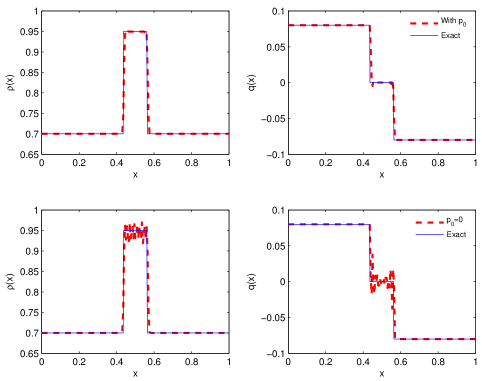
    In Figure 5, the numerical solutions obtained by the Direct method with and without p0subscript𝑝0p_{0} are compared. This confirms the observation made in [18] for the low Mach number limit.
    Refer to caption
    Figure 5: The numerical results of the Direct method with and without p0subscript𝑝0p_{0} for problem (P1’) at t=0.2𝑡0.2t=0.2 with ε=104,Δx=5×10³,Δt=5×10⁴formulae-sequence𝜀superscript104formulae-sequenceΔ𝑥5superscript103Δ𝑡5superscript104\varepsilon=10^{-4},\Delta x=5\times 10^{-3},\Delta t=5\times 10^{-4}. The solid lines are the exact solutions. The dashed curves are the numerical solutions. The left graphs are for ρ𝜌\rho, the right ones for q𝑞q, both as functions of x𝑥x.

    It can be seen that a lot of extra oscillations appear in the numerical solutions when there is no splitting of pressure p (p0=0,p1=pformulae-sequencesubscript𝑝00subscript𝑝1𝑝p_{0}=0,p_{1}=p). That is the reason why we should add a p0subscript𝑝0p_{0} term in the explicit part of the numerical scheme.

Example 2. The Riemann problem (P2)𝑃2(P2) is obtained by exchanging the left and right states of Riemann problem (P1)𝑃1(P1). So the solution to the problem (P2)𝑃2(P2) consists of two rarefaction waves and a vacuum state appears as the intermediate state. As shown in proposition 4, these two rarefaction waves tend to be contact waves.

As in example 1, We choose ε=104,Δx=5×10³,Δt=5×10⁴formulae-sequence𝜀superscript104formulae-sequenceΔ𝑥5superscript103Δ𝑡5superscript104\varepsilon=10^{-4},\Delta x=5\times 10^{-3},\Delta t=5\times 10^{-4}. t=0.0005.

Refer to caption
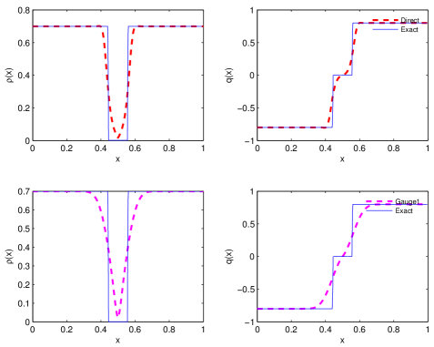
Figure 6: The Direct and Gauge 1 methods for problem (P2) at t=0.05𝑡0.05t=0.05 with ε=104,Δx=5×10³,Δt=5×10⁴formulae-sequence𝜀superscript104formulae-sequenceΔ𝑥5superscript103Δ𝑡5superscript104\varepsilon=10^{-4},\Delta x=5\times 10^{-3},\Delta t=5\times 10^{-4}. The solid lines are the exact solutions. The dashed curves are the numerical solutions. The left graphs are for ρ𝜌\rho, the right ones for q𝑞q, both as functions of x𝑥x.

It can be seen from Figure 6 that the Direct method captures the vacuum and rarefaction waves well. In comparison, the Gauge 1 method as illustrated in Figure 6 shows larger diffusion.

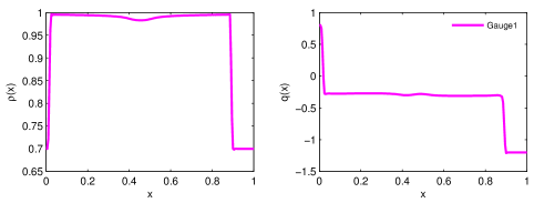
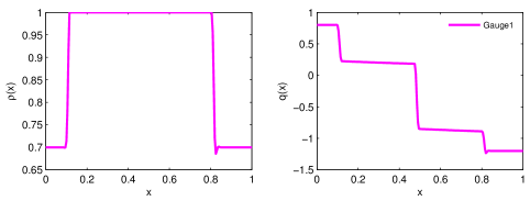
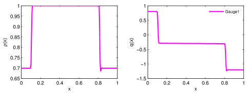
Example 3. The solution to the problem (P3)𝑃3(P3) consists of two Riemann problems: both of them are like the Riemann problem in (P1). So there are two congested regions and eventually they will collide. We are interested in observing how the numerical methods behave at collision. We fix Δx=5×10³,Δt=5×10⁴formulae-sequenceΔ𝑥5superscript103Δ𝑡5superscript104\Delta x=5\times 10^{-3},\Delta t=5\times 10^{-4} and choose ε=104𝜀superscript104\varepsilon=10^{-4} and 108superscript10810^{-8}. Since only shocks are involved, we will use the Gauge 1 method only.
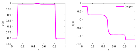
Refer to caption
(a) t=0.0790𝑡0.0790t=0.0790
Refer to caption
(b) t=0.1030𝑡0.1030t=0.1030
Figure 7: Gauge 1 method for problem (P3) with ε=104,Δx=5×10³,Δt=5×10⁴formulae-sequence𝜀superscript104formulae-sequenceΔ𝑥5superscript103Δ𝑡5superscript104\varepsilon=10^{-4},\Delta x=5\times 10^{-3},\Delta t=5\times 10^{-4}. The left graphs are for ρ𝜌\rho, the right ones for q𝑞q, both as functions of x𝑥x.
Refer to caption
(a) t=0.0810𝑡0.0810t=0.0810
Refer to caption
(b) t=0.0815𝑡0.0815t=0.0815
Figure 8: Gauge 1 method for problem (P3) with ε=108,Δx=5×10³,Δt=5×10⁴formulae-sequence𝜀superscript108formulae-sequenceΔ𝑥5superscript103Δ𝑡5superscript104\varepsilon=10^{-8},\Delta x=5\times 10^{-3},\Delta t=5\times 10^{-4}. The left graphs are for ρ𝜌\rho, the right ones for q𝑞q, both as functions of x𝑥x.

From Figures 7 and 8, as ε𝜀\varepsilon becomes smaller, it takes shorter time to form a new congestion region from the two colliding congestion regions: from 484848 time steps to no more than one time step. It can be seen that as ε0𝜀0\varepsilon\to 0, the collision of these two congested shocks aggregate instantaneously.

Example 4. The solution to the Riemann problem (P4)𝑃4(P4) consists of two shocks with intermediate state away from the congestion density. So in the second Riemann problem there are two rarefaction waves and a vacuum state appears as the intermediate state. As shown in section 2, these two rarefaction waves tend to be contact waves.

As above, we choose ε=104,Δx=5×10³,Δt=5×10⁴formulae-sequence𝜀superscript104formulae-sequenceΔ𝑥5superscript103Δ𝑡5superscript104\varepsilon=10^{-4},\Delta x=5\times 10^{-3},\Delta t=5\times 10^{-4}.

Refer to caption
Figure 9: The Direct and Gauge 1 methods for problem (P4) at t=0.2𝑡0.2t=0.2 with ε=104,Δx=5×10³,Δt=5×10⁴formulae-sequence𝜀superscript104formulae-sequenceΔ𝑥5superscript103Δ𝑡5superscript104\varepsilon=10^{-4},\Delta x=5\times 10^{-3},\Delta t=5\times 10^{-4}. The solid lines are the exact solutions. The dashed curves are the numerical solutions. The left graphs are for ρ𝜌\rho, the right ones for q𝑞q, both as functions of x𝑥x.

It can be seen from Figure 9 that the Direct method performs well when the density is far away from congestion. However, the Gauge 1 method does not work well possibly due to the extra diffusion.

Remark 2

All the features described above are preserved when we apply the fully implicit method (21)(22)(implicit in both ρ𝜌\rho and qqρtensor-product𝑞𝑞𝜌\frac{q\otimes q}{\rho}) to the Direct and Gauge 1 method. There is a little improvement in the accuracy but no major one.

Finally, we can compare the Gauge 1 and Gauge 2 methods. With the stencil of (46) in the same setting as that of example 2, the Gauge 2 method yields almost the same numerical result as the Direct method (see Fig. 10).
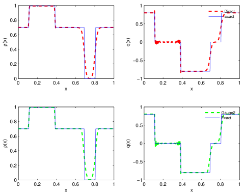
Refer to caption
Figure 10: The Direct and Gauge 2 methods with discretization (43) for problem (P2) at t=0.05𝑡0.05t=0.05. The solid lines are the exact solutions. The dashed curves are the numerical solutions. The left graphs are for ρ𝜌\rho, the right ones for q𝑞q, both as functions of x𝑥x.

5.2 A two dimensional test case

In this section, we will test the Direct and Gauge 1 method in the 2D case. Since there is no theoretical solution in 2D case, only some phenomena will be presented.

The test example is chosen to illustrate the collision of two congested regions. It is basically a two dimensional extension of the test case (P3) with some lateral shift. The initial data of the density and velocity is:

ρ=0.8×1AB+0.6×1[0,1]×[0,1]\(AB),𝜌0.8subscript1𝐴𝐵0.6subscript1\0101𝐴𝐵\displaystyle\rho=0.8\times\mathrm{1}_{A\cup B}+0.6\times\mathrm{1}_{[0,1]\times[0,1]\backslash(A\cup B)}, (59)
𝒒(x,y,0)=(10)1A+(10)1B,𝒒𝑥𝑦0matrix10subscript1𝐴matrix10subscript1𝐵\displaystyle\boldsymbol{q}(x,y,0)=\begin{pmatrix}1\\ 0\end{pmatrix}\mathrm{1}_{A}+\begin{pmatrix}-1\\ 0\end{pmatrix}\mathrm{1}_{B}, (60)
A=[16,512]×[13,712],B=[712,56]×[512,23].formulae-sequence𝐴1651213712𝐵7125651223\displaystyle A=\left[\frac{1}{6},\frac{5}{12}\right]\times\left[\frac{1}{3},\frac{7}{12}\right],\quad B=\left[\frac{7}{12},\frac{5}{6}\right]\times\left[\frac{5}{12},\frac{2}{3}\right]. (61)

The vector field q𝑞q is plotted in the Figure 11.

Remark 3

In this test example, the background density is ρ=0.6𝜌0.6\rho=0.6. It is even more interesting to see what happens when the background density is close to zero. However, our schemes are not performing well in this situation. Indeed, vacuum is a big problem which needs some special treatment. And when the background density is close to zero, the system is almost pressureless, which is also a difficult problem. These problems may be considered in the future work.
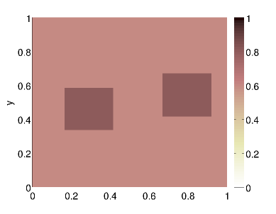
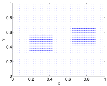
Refer to caption
(a) density ρ𝜌\rho
Refer to caption
(b) vector field of momentum 𝒒𝒒\boldsymbol{q}
Figure 11: The initial data of the density and momentum 𝒒𝒒\boldsymbol{q}, both as functions of x𝑥x and y𝑦y.

It can be expected that there will be two congested regions forming and moving towards each other with two shocks in the front and two rarefaction waves left behind. These two shocks compress the fluid and cause congestion. This is reflected in Figure 12.
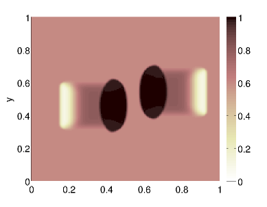
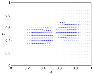
Refer to caption
(a) density ρ𝜌\rho
Refer to caption
(b) vector field of momentum 𝒒𝒒\boldsymbol{q}
Figure 12: The Direct method with ε=104,Δx=5×10³,Δt=5×10⁴formulae-sequence𝜀superscript104formulae-sequenceΔ𝑥5superscript103Δ𝑡5superscript104\varepsilon=10^{-4},\Delta x=5\times 10^{-3},\Delta t=5\times 10^{-4} at t=0.05𝑡0.05t=0.05. The left graph is for ρ𝜌\rho, the right one for vector field q𝑞q, both as functions of x𝑥x and y𝑦y.

These two shocks with opposite directions meet at a later time. The interaction of these shocks forms a bigger congestion region with higher density, which can be illustrated in Figure 13. The interaction of the two shocks induces the formation of two new shocks moving in the orthogonal direction compared to the initial motion.
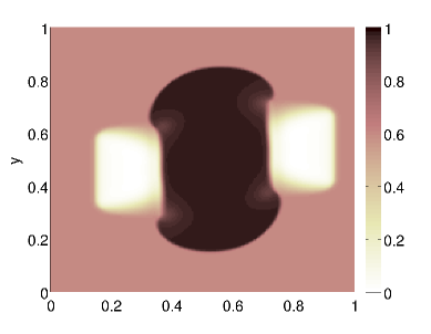
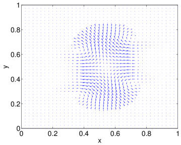
Refer to caption
(a) density ρ𝜌\rho
Refer to caption
(b) vector field of momentum 𝒒𝒒\boldsymbol{q}
Figure 13: The Direct method with ε=104,Δx=5×10³,Δt=5×10⁴formulae-sequence𝜀superscript104formulae-sequenceΔ𝑥5superscript103Δ𝑡5superscript104\varepsilon=10^{-4},\Delta x=5\times 10^{-3},\Delta t=5\times 10^{-4} at t=0.2𝑡0.2t=0.2. The left graph is for ρ𝜌\rho, the right one for vector field q𝑞q, both as functions of x𝑥x and y𝑦y.

The similar result can be obtained by the Gauge 1 method as in Figure 14 and 15.

Refer to caption
(a) density ρ𝜌\rho
Refer to caption
(b) vector field of momentum 𝒒𝒒\boldsymbol{q}
Figure 14: The Gauge 1 method with ε=104,Δx=5×10³,Δt=5×10⁴formulae-sequence𝜀superscript104formulae-sequenceΔ𝑥5superscript103Δ𝑡5superscript104\varepsilon=10^{-4},\Delta x=5\times 10^{-3},\Delta t=5\times 10^{-4} at t=0.05𝑡0.05t=0.05. The left graph is for ρ𝜌\rho, the right one for vector field q𝑞q, both as functions of x𝑥x and y𝑦y.
Refer to caption
(a) density ρ𝜌\rho
Refer to caption
(b) vector field of momentum 𝒒𝒒\boldsymbol{q}
Figure 15: The Gauge 1 method with ε=104,Δx=5×10³,Δt=5×10⁴formulae-sequence𝜀superscript104formulae-sequenceΔ𝑥5superscript103Δ𝑡5superscript104\varepsilon=10^{-4},\Delta x=5\times 10^{-3},\Delta t=5\times 10^{-4} at t=0.2𝑡0.2t=0.2. The left graph is for ρ𝜌\rho, the right one for vector field q𝑞q, both as functions of x𝑥x and y𝑦y.

The difference between the two methods in the two dimensional case is not striking. In order to illustrate them, we look at a cut at y=0.5𝑦0.5y=0.5. The cuts are displayed on Figure 16 and 17.
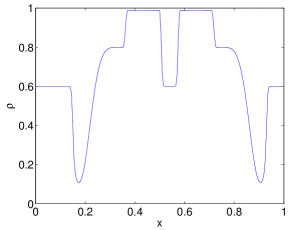
Refer to caption
(a) Direct method
Refer to caption
(b) Gauge 1 method
Figure 16: Direct and Gauge 1 methods with ε=104,Δx=5×10³,Δt=5×10⁴formulae-sequence𝜀superscript104formulae-sequenceΔ𝑥5superscript103Δ𝑡5superscript104\varepsilon=10^{-4},\Delta x=5\times 10^{-3},\Delta t=5\times 10^{-4} at t=0.05𝑡0.05t=0.05. Cut of the density along the line y=0.5𝑦0.5y=0.5, as a function of x𝑥x. Left hand: Direct method; right hand: Gauge 1 method.
Refer to caption
(a) Direct method
Refer to caption
(b) Gauge 1 method
Figure 17: Momentum of the Direct and Gauge 1 methods with ε=104,Δx=5×10³,Δt=5×10⁴formulae-sequence𝜀superscript104formulae-sequenceΔ𝑥5superscript103Δ𝑡5superscript104\varepsilon=10^{-4},\Delta x=5\times 10^{-3},\Delta t=5\times 10^{-4} at t=0.05𝑡0.05t=0.05. Cut of the momentum along the line y=0.5𝑦0.5y=0.5, as a function of x𝑥x. Left hand: Direct method; right hand: Gauge 1 method.

Similar observations as in the one dimensional case can be made from Figure 16 and 17. The Gauge 1 method provides a little less oscillations in the congestion region but also brings more diffusion.

6 Conclusion

In this paper, we have studied the Euler system with a maximal density constraint. A small parameter ε𝜀\varepsilon was introduced to measure the stiffness of the constraint. As ε0𝜀0\varepsilon\rightarrow 0, the model gives rise to a two-phase model with congested regions (with maximal density) and uncongested regions (with density below the maximal density).

One-dimensional solutions of this asymptotic problem have been investigated to provide the information of the interface conditions. However, it can not characterize the whole dynamics and it is hard to extend to higher dimensional cases. Therefore, we have devised asymptotic preserving numerical schemes, which are valid for all range of ε𝜀\varepsilon and thus are capable of capturing the asymptotic dynamics. Two numerical schemes have been considered and compared on both one-dimensional and two dimensional test-cases. They both capture the congested regions well. However, the first method shows some oscillations near the interface between congested and uncongested regions, while the second has much less oscillations but is more diffusive. A careful error analysis in different norms with respect to different parameters (time and space steps, ε𝜀\varepsilon) are conducted for a one dimensional test case.

Following [35], the development of second order schemes will be performed in future works. More robust schemes for capturing the divergence free constraint in the congested regions could also be investigated. Coupling our methodology with schemes dedicated to the pressureless gas dynamics could also improve the results in the low density regions. Finally, simulations of the non-conservative model with a supplementary geometric constraint on the speed of the flow [17] will be an interesting problem.

Acknowledgement This work has been supported by the Marie Curie Actions of the European Commission in the frame of the DEASE project (MEST-CT-2005-021122), by the Agence Nationale de la Recherche (ANR) under contracts PANURGE (ANR-07-BLAN-0208-03) and PEDIGREE (ANR-08-SYSC-015-01).

A Appendix : Solutions of the one-dimensional problem: the Riemann problem and the cluster collisions

The one-dimensional version of system (4)-(5) can be written as follows:

tρ+xq=0,subscript𝑡𝜌subscript𝑥𝑞0\displaystyle\partial_{t}\rho+\partial_{x}q=0, (62)
tq+x(q2ρ)+x(εp(ρ))=0,subscript𝑡𝑞subscript𝑥superscript𝑞2𝜌subscript𝑥𝜀𝑝𝜌0\displaystyle\partial_{t}q+\partial_{x}\left(\frac{q^{2}}{\rho}\right)+\partial_{x}(\varepsilon p(\rho))=0, (63)

where q(x,t)𝑞𝑥𝑡q(x,t) is here a scalar function and x𝑥x is the position in \mathbb{R}. In this section, we first investigate the Riemann problem and the limits of its solutions as ε0𝜀0\varepsilon\rightarrow 0 and then we briefly recall the one-dimensional solutions of the limit system (8)-(9)-(10) provided in [12], which consists of the collision of two finite clusters (domain where ρ=ρ𝜌superscript𝜌\rho=\rho^{\ast}).

A.1 The one-dimensional Riemann problem

The Riemann problem is an initial value problem, where the initial condition is a piece-wise constant function with a discontinuity between two constant states:

(ρ0,q0)(x)={(ρ,q), for x<0,(ρr,qr), for x0.subscript𝜌0subscript𝑞0𝑥casessubscript𝜌subscript𝑞 for 𝑥0missing-subexpressionsubscript𝜌𝑟subscript𝑞𝑟 for 𝑥0missing-subexpression(\rho_{0},q_{0})(x)=\left\{\begin{array}[]{cl}(\rho_{\ell},q_{\ell}),\text{ for }x<0,\\ (\rho_{r},q_{r}),\text{ for }x\geq 0.\end{array}\right.

The solutions of this problem for the Euler system (62)-(63) are well known. So, the strategy is to take the limits of these solutions as ε𝜀\varepsilon goes to zero. This provides the solutions of the Riemann problem for the singular asymptotic limit (8)-(9)-(10). Similar studies was carried out in [5] for the isentropic Euler equation, in [9] for a traffic jam model and in [17] for a herding problem.

A.1.1 Shock and rarefaction waves

The material of this section is classical, and is given here only for the reader’s convenience.

The two characteristic speeds λ±εsuperscriptsubscript𝜆plus-or-minus𝜀\lambda_{\pm}^{\varepsilon} and the two characteristic fields 𝒓±εsuperscriptsubscript𝒓plus-or-minus𝜀\boldsymbol{r}_{\pm}^{\varepsilon} of the one-dimensional system (62)-(63) are:

λ±ε=u±εp(ρ),𝒓±ε=(1u±εp(ρ)).formulae-sequencesuperscriptsubscript𝜆plus-or-minus𝜀plus-or-minus𝑢𝜀superscript𝑝𝜌superscriptsubscript𝒓plus-or-minus𝜀1plus-or-minus𝑢𝜀superscript𝑝𝜌\lambda_{\pm}^{\varepsilon}=u\pm\sqrt{\varepsilon p^{\prime}(\rho)},\quad\boldsymbol{r}_{\pm}^{\varepsilon}=\left(\begin{array}[]{c}1\\ u\pm\sqrt{\varepsilon p^{\prime}(\rho)}\end{array}\right).

It can be easily checked that both characteristic fields are genuinely non linear for positive densities. Therefore, the solutions of the Riemann problem are made of constant states separated by rarefaction or shock waves [27].

The rarefaction waves are continuous self similar solutions: (ρ(x/t),q(x/t))𝜌𝑥𝑡𝑞𝑥𝑡(\rho(x/t),q(x/t)). Given a state (ρ^,q^)^𝜌^𝑞(\hat{\rho},\hat{q}), the states which can be connected to (ρ^,q^)^𝜌^𝑞(\hat{\rho},\hat{q}) by a rarefaction wave are those located on the integral curves i±εsuperscriptsubscript𝑖plus-or-minus𝜀i_{\pm}^{\varepsilon} of the right eigenvectors of the Jacobian matrix of the flux function issued from (ρ^,q^)^𝜌^𝑞(\hat{\rho},\hat{q}). They are given by:

ρ(s)=1,i±ε(s)=u^±εp(ρ),ρ(0)=ρ^,i±ε(0)=q^,formulae-sequencesuperscript𝜌𝑠1formulae-sequencesuperscriptsubscript𝑖plus-or-minussuperscript𝜀𝑠plus-or-minus^𝑢𝜀superscript𝑝𝜌formulae-sequence𝜌0^𝜌superscriptsubscript𝑖plus-or-minus𝜀0^𝑞\rho^{\prime}(s)=1,\quad i_{\pm}^{\varepsilon\ ^{\prime}}(s)=\hat{u}\pm\sqrt{\varepsilon p^{\prime}(\rho)},\quad\rho(0)=\hat{\rho},\quad i_{\pm}^{\varepsilon}(0)=\hat{q},

which is equivalent to i±ε(ρ)=u^±εp(ρ),i±ε(ρ^)=q^formulae-sequencesuperscriptsubscript𝑖plus-or-minussuperscript𝜀𝜌plus-or-minus^𝑢𝜀superscript𝑝𝜌superscriptsubscript𝑖plus-or-minus𝜀^𝜌^𝑞i_{\pm}^{\varepsilon\ ^{\prime}}(\rho)=\hat{u}\pm\sqrt{\varepsilon p^{\prime}(\rho)},\ i_{\pm}^{\varepsilon}(\hat{\rho})=\hat{q} and then to equation:

i±ε(ρ)=ρu^±ρε(P(ρ)P(ρ^)),superscriptsubscript𝑖plus-or-minus𝜀𝜌plus-or-minus𝜌^𝑢𝜌𝜀𝑃𝜌𝑃^𝜌i_{\pm}^{\varepsilon}(\rho)=\rho\hat{u}\pm\rho\sqrt{\varepsilon}(P(\rho)-P(\hat{\rho})), (64)

where P𝑃P is an antiderivative of p(u)/usuperscript𝑝𝑢𝑢\sqrt{p^{\prime}(u)}/u and u^=q^/ρ^^𝑢^𝑞^𝜌\hat{u}=\hat{q}/\hat{\rho}. The graph of iεsuperscriptsubscript𝑖𝜀i_{-}^{\varepsilon} (resp. i+εsuperscriptsubscript𝑖𝜀i_{+}^{\varepsilon}) is called the 1-integral curve (resp. the 2-integral curve). The following proposition provides several features of the integral curves.

Proposition 1

(Integral and rarefaction curves)

  1. 1.

    The 1-integral curve iεsuperscriptsubscript𝑖𝜀i_{-}^{\varepsilon} (resp. the 2-integral curve i+εsuperscriptsubscript𝑖𝜀i_{+}^{\varepsilon}) is concave (resp. convex) as functions of ρ𝜌\rho and iε(0)=i+ε(0)=0superscriptsubscript𝑖𝜀0superscriptsubscript𝑖𝜀00i_{-}^{\varepsilon}(0)=i_{+}^{\varepsilon}(0)=0.

  2. 2.

    The limit of the integral curves as ε𝜀\varepsilon goes to zero is the union of the straight lines {q=ρu^}𝑞𝜌^𝑢\left\{q=\rho\hat{u}\right\} and {ρ=ρ}𝜌superscript𝜌\left\{\rho=\rho^{\ast}\right\}.

  3. 3.

    Suppose that the state ρ^εsuperscript^𝜌𝜀\hat{\rho}^{\varepsilon} is such that ρ^ερsuperscript^𝜌𝜀superscript𝜌\hat{\rho}^{\varepsilon}\rightarrow\rho^{\ast} and εp(ρ^ε)p¯𝜀𝑝superscript^𝜌𝜀¯𝑝\varepsilon p(\hat{\rho}^{\varepsilon})\rightarrow\bar{p}. For all ρ<ρ^ε𝜌superscript^𝜌𝜀\rho<\hat{\rho}^{\varepsilon}, we have:

    |i±ε(ρ)ρu^|ε0ρ^εp(u)u𝑑u=Oρ^ερ(ε12γ)superscriptsubscript𝑖plus-or-minus𝜀𝜌𝜌^𝑢𝜀superscriptsubscript0superscript^𝜌𝜀superscript𝑝𝑢𝑢differential-d𝑢superscript^𝜌𝜀superscript𝜌𝑂superscript𝜀12𝛾\quad\left|\frac{i_{\pm}^{\varepsilon}(\rho)}{\rho}-\hat{u}\right|\leq\sqrt{\varepsilon}\int_{0}^{\hat{\rho}^{\varepsilon}}\frac{\sqrt{p^{\prime}(u)}}{u}du=\underset{\hat{\rho}^{\varepsilon}\rightarrow\rho^{\ast}}{O}(\varepsilon^{\frac{1}{2\gamma}})
  4. 4.

    If (ρ^,q^)^𝜌^𝑞(\hat{\rho},\hat{q}) is a left state, the right states which can be connected to it by a rarefaction wave are those located on the 1-rarefaction curve {(ρ,iε(ρ)),ρ<ρ^}𝜌superscriptsubscript𝑖𝜀𝜌𝜌^𝜌\left\{(\rho,i_{-}^{\varepsilon}(\rho)),\ \rho<\hat{\rho}\right\} or the 2-rarefaction curve {(ρ,i+ε(ρ)),ρ>ρ^}𝜌superscriptsubscript𝑖𝜀𝜌𝜌^𝜌\left\{(\rho,i_{+}^{\varepsilon}(\rho)),\ \rho>\hat{\rho}\right\}.

The last point of this proposition stems from the compatibility conditions of the characteristic speeds. The proof of this proposition is classical and omitted.
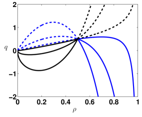
A shock wave is a discontinuity between two constant states, (ρ^,q^)^𝜌^𝑞(\hat{\rho},\hat{q}) and (ρ,q)𝜌𝑞(\rho,q), travelling at constant speed σ𝜎\sigma. The states (ρ,q)𝜌𝑞(\rho,q), which can be connected to (ρ^,q^)^𝜌^𝑞(\hat{\rho},\hat{q}) by a shock wave, are determined by the Rankine-Hugoniot conditions:

[q]=σ[ρ],[q2ρ+εp(ρ)]=σ[q],formulae-sequencedelimited-[]𝑞𝜎delimited-[]𝜌delimited-[]superscript𝑞2𝜌𝜀𝑝𝜌𝜎delimited-[]𝑞[q]=\sigma[\rho],\quad\left[\frac{q^{2}}{\rho}+\varepsilon p(\rho)\right]=\sigma[q], (65)

where [f]:=ff^assigndelimited-[]𝑓𝑓^𝑓[f]:=f-\hat{f} for all quantities f𝑓f. Easy computations show that the admissible states are of the form (ρ,h±ε(ρ))𝜌superscriptsubscriptplus-or-minus𝜀𝜌(\rho,h_{\pm}^{\varepsilon}(\rho)), where h±εsuperscriptsubscriptplus-or-minus𝜀h_{\pm}^{\varepsilon} is :

h±ε(ρ)=u^±ρρ^(ρρ^)(εp(ρ)εp(ρ^)).superscriptsubscriptplus-or-minus𝜀𝜌plus-or-minus^𝑢𝜌^𝜌𝜌^𝜌𝜀𝑝𝜌𝜀𝑝^𝜌h_{\pm}^{\varepsilon}(\rho)=\hat{u}\pm\sqrt{\frac{\rho}{\hat{\rho}}}\sqrt{(\rho-\hat{\rho})(\varepsilon p(\rho)-\varepsilon p(\hat{\rho}))}. (66)

and the shock speeds are:

σ±=(h±ε(ρ)q^)(ρρ^)=u^±ρρ^(εp(ρ)εp(ρ^))(ρρ^).subscript𝜎plus-or-minussuperscriptsubscriptplus-or-minus𝜀𝜌^𝑞𝜌^𝜌plus-or-minus^𝑢𝜌^𝜌𝜀𝑝𝜌𝜀𝑝^𝜌𝜌^𝜌\sigma_{\pm}=\frac{(h_{\pm}^{\varepsilon}(\rho)-\hat{q})}{(\rho-\hat{\rho})}=\hat{u}\pm\sqrt{\frac{\rho}{\hat{\rho}}}\sqrt{\frac{(\varepsilon p(\rho)-\varepsilon p(\hat{\rho}))}{(\rho-\hat{\rho})}}. (67)

The graph of hεsuperscriptsubscript𝜀h_{-}^{\varepsilon} (resp. h+εsuperscriptsubscript𝜀h_{+}^{\varepsilon}) is called the 1-Hugoniot curve (resp. the 2-Hugoniot curve). The following proposition provides several properties of the Hugoniot curves:

Proposition 2

(Hugoniot and shock curves)

  1. 1.

    The 1-Hugoniot function hεsuperscriptsubscript𝜀h_{-}^{\varepsilon} (resp. the 2-Hugoniot function h+εsuperscriptsubscript𝜀h_{+}^{\varepsilon}) is concave (resp. convex) and hε(0)=h+ε(0)=0superscriptsubscript𝜀0superscriptsubscript𝜀00h_{-}^{\varepsilon}(0)=h_{+}^{\varepsilon}(0)=0.

  2. 2.

    The limits of the graphs of hεsuperscriptsubscript𝜀h_{-}^{\varepsilon} and h+εsuperscriptsubscript𝜀h_{+}^{\varepsilon} when ε𝜀\varepsilon goes to zero are the union of the straight lines {q=ρu^}𝑞𝜌^𝑢\left\{q=\rho\hat{u}\right\} and {ρ=ρ}𝜌superscript𝜌\left\{\rho=\rho^{\ast}\right\}. This is true also when ρ^=ρ^ε^𝜌superscript^𝜌𝜀\hat{\rho}=\hat{\rho}^{\varepsilon} depends on ε𝜀\varepsilon and tends to ρsuperscript𝜌\rho^{\ast}.

  3. 3.

    If (ρ^,q^)^𝜌^𝑞(\hat{\rho},\hat{q}) is a left state, the right states which can be connected to it by an entropic shock wave are those located on the 1-shock curve {(ρ,hε(ρ)),ρ>ρ^}𝜌superscriptsubscript𝜀𝜌𝜌^𝜌\left\{(\rho,h_{-}^{\varepsilon}(\rho)),\ \rho>\hat{\rho}\right\} or the 2-shock curve {(ρ,h+ε(ρ)),ρ<ρ^}𝜌superscriptsubscript𝜀𝜌𝜌^𝜌\left\{(\rho,h_{+}^{\varepsilon}(\rho)),\ \rho<\hat{\rho}\right\}.

The proof of this proposition is classical and omitted.

Refer to caption
Figure 18: Curves issued from (ρ^,q^)=(0.5,0.5)^𝜌^𝑞0.50.5(\hat{\rho},\hat{q})=(0.5,0.5) and ε{10,1,102}𝜀101superscript102\varepsilon\in\left\{10,1,10^{-2}\right\}. In dotted line : the rarefaction curves. In solid line : the shock curves. In blue : the 1-curves. In black : the 2-curves. As ε0𝜀0\varepsilon\rightarrow 0, the curves are tending to the straight lines {q=u^ρ}𝑞^𝑢𝜌\left\{q=\hat{u}\rho\right\} and {ρ=ρ}𝜌superscript𝜌\left\{\rho=\rho^{\ast}\right\}. Parameters : k=2,ρ=1formulae-sequence𝑘2superscript𝜌1k=2,\rho^{\ast}=1.

A.1.2 The Riemann problem for system (62)-(63)

Geometric considerations on the intersection of the integral and Hugoniot curves enable us to solve the Riemann problem [27]. These arguments are really simplified in the limit ε0𝜀0\varepsilon\rightarrow 0, due to the much simpler behaviour of the integral and Hugoniot curves: they both converge to union of the straight lines {q=ρu^}𝑞𝜌^𝑢\left\{q=\rho\hat{u}\right\} and {ρ=ρ}𝜌superscript𝜌\left\{\rho=\rho^{\ast}\right\}. This behaviour is illustrated in Fig. 18. The following proposition provides the nature of the solutions of the Riemann problem for ε𝜀\varepsilon small enough. It depends on the sign of the relative velocity uursubscript𝑢subscript𝑢𝑟u_{\ell}-u_{r}, where u=q/ρsubscript𝑢subscript𝑞subscript𝜌u_{\ell}=q_{\ell}/\rho_{\ell} and ur=qr/ρrsubscript𝑢𝑟subscript𝑞𝑟subscript𝜌𝑟u_{r}=q_{r}/\rho_{r}:

Proposition 3

Let (ρ,q)subscript𝜌subscript𝑞(\rho_{\ell},q_{\ell}), (ρr,qr)subscript𝜌𝑟subscript𝑞𝑟(\rho_{r},q_{r}), left and right states. Then the solutions of the Riemann problem related to (62)-(63) have the following forms:

  1. 1.

    If u<ursubscript𝑢subscript𝑢𝑟u_{\ell}<u_{r}, then for ε𝜀\varepsilon small enough, the intermediate state is the intersection point of the 1-integral curve issued from (ρ,q,p¯)subscript𝜌subscript𝑞subscript¯𝑝(\rho_{\ell},q_{\ell},\bar{p}_{\ell}) and the 2-integral curve issued from (ρr,qr,p¯r)subscript𝜌𝑟subscript𝑞𝑟subscript¯𝑝𝑟(\rho_{r},q_{r},\bar{p}_{r}). Besides, the intermediate density ρ~~𝜌\tilde{\rho} is lower than ρrsubscript𝜌𝑟\rho_{r} and ρsubscript𝜌\rho_{\ell}. This is valid even if ρsubscript𝜌\rho_{\ell} or/and ρrsubscript𝜌𝑟\rho_{r} tends to ρsuperscript𝜌\rho^{\ast}.

  2. 2.

    If u>ursubscript𝑢subscript𝑢𝑟u_{\ell}>u_{r}, then for ε𝜀\varepsilon small enough, there are two subcases:

    • if hε(ρrε)>qrsuperscriptsubscript𝜀superscriptsubscript𝜌𝑟𝜀subscript𝑞𝑟h_{-}^{\varepsilon}(\rho_{r}^{\varepsilon})>q_{r} and h+ε(ρε)<qsuperscriptsubscript𝜀superscriptsubscript𝜌𝜀subscript𝑞h_{+}^{\varepsilon}(\rho_{\ell}^{\varepsilon})<q_{\ell}, the intermediate state is the intersection point of the 1-Hugoniot curve issued from (ρ,q)subscript𝜌subscript𝑞(\rho_{\ell},q_{\ell}) and the 2-Hugoniot curve issued from (ρr,qr)subscript𝜌𝑟subscript𝑞𝑟(\rho_{r},q_{r}).

    • if hε(ρrε)<qrsuperscriptsubscript𝜀superscriptsubscript𝜌𝑟𝜀subscript𝑞𝑟h_{-}^{\varepsilon}(\rho_{r}^{\varepsilon})<q_{r} (resp. h+ε(ρε)>qsuperscriptsubscript𝜀superscriptsubscript𝜌𝜀subscript𝑞h_{+}^{\varepsilon}(\rho_{\ell}^{\varepsilon})>q_{\ell}), the intermediate state is the intersection point of the 1-Hugoniot curve (resp. 1-integral curve) issued from (ρ,q)subscript𝜌subscript𝑞(\rho_{\ell},q_{\ell}) and the 2-integral curve (resp. 2-Hugoniot curve) issued from (ρr,qr)subscript𝜌𝑟subscript𝑞𝑟(\rho_{r},q_{r}).

  3. 3.

    If ur=usubscript𝑢𝑟subscript𝑢u_{r}=u_{\ell} and ρ<ρrsubscript𝜌subscript𝜌𝑟\rho_{\ell}<\rho_{r} (resp. ρ>ρrsubscript𝜌subscript𝜌𝑟\rho_{\ell}>\rho_{r}), then the intermediate state is the intersection point of the 1-Hugoniot curve (resp. 1-integral curve) issued from (ρ,q,p¯)subscript𝜌subscript𝑞subscript¯𝑝(\rho_{\ell},q_{\ell},\bar{p}_{\ell}) and the 2-integral curve (resp. 2-Hugoniot curve) issued from (ρr,qr,p¯r)subscript𝜌𝑟subscript𝑞𝑟subscript¯𝑝𝑟(\rho_{r},q_{r},\bar{p}_{r}). Besides, the intermediate density ρ~~𝜌\tilde{\rho} is the interval [ρ,ρr]subscript𝜌subscript𝜌𝑟[\rho_{\ell},\rho_{r}] (resp. [ρr,ρ]subscript𝜌𝑟subscript𝜌[\rho_{r},\rho_{\ell}]). This is valid even if ρsubscript𝜌\rho_{\ell} or/and ρrsubscript𝜌𝑟\rho_{r} tends to ρsuperscript𝜌\rho^{\ast}.

This proposition results from propositions 1 and 2. The proof is omitted here (it is an easy adaptation of the proof of Theorem 1 in [17]). Note that the nature of the curves (integral or Hugoniot curve) implies the nature of the waves involved in the Riemann problem.

A.1.3 The limits of solutions of the Riemann problem.

We introduce the following initial conditions:

(ρ0ε,q0ε)(x)={(ρε,qε), for x<0,(ρrε,qrε), for x0.superscriptsubscript𝜌0𝜀superscriptsubscript𝑞0𝜀𝑥casessuperscriptsubscript𝜌𝜀superscriptsubscript𝑞𝜀 for 𝑥0missing-subexpressionsuperscriptsubscript𝜌𝑟𝜀superscriptsubscript𝑞𝑟𝜀 for 𝑥0missing-subexpression(\rho_{0}^{\varepsilon},q_{0}^{\varepsilon})(x)=\left\{\begin{array}[]{cl}(\rho_{\ell}^{\varepsilon},q_{\ell}^{\varepsilon}),\text{ for }x<0,\\ (\rho_{r}^{\varepsilon},q_{r}^{\varepsilon}),\text{ for }x\geq 0.\end{array}\right.

with (ρε,qε,εp(ρε))(ρ,q,p¯)superscriptsubscript𝜌𝜀superscriptsubscript𝑞𝜀𝜀𝑝superscriptsubscript𝜌𝜀subscript𝜌subscript𝑞subscript¯𝑝(\rho_{\ell}^{\varepsilon},q_{\ell}^{\varepsilon},\varepsilon p(\rho_{\ell}^{\varepsilon}))\rightarrow(\rho_{\ell},q_{\ell},\bar{p}_{\ell}) and (ρrε,qrε,εp(ρrε))(ρr,qr,p¯r)superscriptsubscript𝜌𝑟𝜀superscriptsubscript𝑞𝑟𝜀𝜀𝑝superscriptsubscript𝜌𝑟𝜀subscript𝜌𝑟subscript𝑞𝑟subscript¯𝑝𝑟(\rho_{r}^{\varepsilon},q_{r}^{\varepsilon},\varepsilon p(\rho_{r}^{\varepsilon}))\rightarrow(\rho_{r},q_{r},\bar{p}_{r}) as ε𝜀\varepsilon goes to zero.

The following proposition provides the solution when ρ,ρr<ρsubscript𝜌subscript𝜌𝑟superscript𝜌\rho_{\ell},\rho_{r}<\rho^{\ast} and so p¯=p¯r=0subscript¯𝑝subscript¯𝑝𝑟0\bar{p}_{\ell}=\bar{p}_{r}=0. The nature of the solution only depends on the sign of the relative velocity uursubscript𝑢subscript𝑢𝑟u_{\ell}-u_{r}, where u=q/ρsubscript𝑢subscript𝑞subscript𝜌u_{\ell}=q_{\ell}/\rho_{\ell} and ur=qr/ρrsubscript𝑢𝑟subscript𝑞𝑟subscript𝜌𝑟u_{r}=q_{r}/\rho_{r}.

Proposition 4

(case ρ<ρ,ρr<ρformulae-sequencesubscriptρsuperscriptρsubscriptρrsuperscriptρ\rho_{\ell}<\rho^{\ast},\rho_{r}<\rho^{\ast})

  1. 1.

    If uur<0subscript𝑢subscript𝑢𝑟0u_{\ell}-u_{r}<0, then the solution consists of two contact waves connecting the two states to the vacuum. This is summarised in the following diagram:

    (ρ,q,0)contact(0,q,0)vacuum(0,qr,0)contact(ρr,qr,0).(\rho_{\ell},q_{\ell},0)\quad\stackrel{{\scriptstyle\mbox{contact}}}{{\longrightarrow}}\quad(0,q_{\ell},0)\stackrel{{\scriptstyle\mbox{vacuum}}}{{\longrightarrow}}\quad(0,q_{r},0)\quad\stackrel{{\scriptstyle\mbox{contact}}}{{\longrightarrow}}\quad(\rho_{r},q_{r},0).
  2. 2.

    If uur>0subscript𝑢subscript𝑢𝑟0u_{\ell}-u_{r}>0, then the solution consists of two shock waves connecting the left state (ρ,q,0)subscript𝜌subscript𝑞0(\rho_{\ell},q_{\ell},0) to an intermediate state (ρ,q~,p¯)superscript𝜌~𝑞¯𝑝(\rho^{\ast},\tilde{q},\bar{p}) and then (ρ,q~,p¯)superscript𝜌~𝑞¯𝑝(\rho^{\ast},\tilde{q},\bar{p}) to the right state (ρr,qr,0)subscript𝜌𝑟subscript𝑞𝑟0(\rho_{r},q_{r},0):

    (ρ,q,0)shock(ρ,q~,p¯)shock(ρr,qr,0),subscript𝜌subscript𝑞0superscriptshocksuperscript𝜌~𝑞¯𝑝superscriptshocksubscript𝜌𝑟subscript𝑞𝑟0(\rho_{\ell},q_{\ell},0)\quad\stackrel{{\scriptstyle\mbox{shock}}}{{\longrightarrow}}\quad(\rho^{\ast},\tilde{q},\bar{p})\quad\stackrel{{\scriptstyle\mbox{shock}}}{{\longrightarrow}}\quad(\rho_{r},q_{r},0),

    where the intermediate momentum q~~𝑞\tilde{q} and the intermediate pressure p¯¯𝑝\bar{p} are:

    q~=uρρρ(ρρ)p¯=urρ+ρρr(ρρr)p¯,~𝑞subscript𝑢superscript𝜌superscript𝜌subscript𝜌superscript𝜌subscript𝜌¯𝑝subscript𝑢𝑟superscript𝜌superscript𝜌subscript𝜌𝑟superscript𝜌subscript𝜌𝑟¯𝑝\displaystyle\tilde{q}=u_{\ell}\rho^{\ast}-\sqrt{\frac{\rho^{\ast}}{\rho_{\ell}}}\sqrt{(\rho^{\ast}-\rho_{\ell})\bar{p}}=u_{r}\rho^{\ast}+\sqrt{\frac{\rho^{\ast}}{\rho_{r}}}\sqrt{(\rho^{\ast}-\rho_{r})\bar{p}},
    p¯=(uur)2(ρρρρ+ρρrρrρ)2,¯𝑝superscriptsubscript𝑢subscript𝑢𝑟2superscriptsuperscript𝜌subscript𝜌subscript𝜌superscript𝜌superscript𝜌subscript𝜌𝑟subscript𝜌𝑟superscript𝜌2\displaystyle\bar{p}=\left(u_{\ell}-u_{r}\right)^{2}\left(\sqrt{\frac{\rho^{\ast}-\rho_{\ell}}{\rho_{\ell}\rho^{\ast}}}+\sqrt{\frac{\rho^{\ast}-\rho_{r}}{\rho_{r}\rho^{\ast}}}\right)^{-2},

    and the shock speeds σsubscript𝜎\sigma_{-} and σ+subscript𝜎\sigma_{+} are given by:

    σ=uρρ(ρρ)p¯,σ+=ur+ρρr(ρρr)p¯.formulae-sequencesubscript𝜎subscript𝑢superscript𝜌subscript𝜌superscript𝜌subscript𝜌¯𝑝subscript𝜎subscript𝑢𝑟superscript𝜌subscript𝜌𝑟superscript𝜌subscript𝜌𝑟¯𝑝\sigma_{-}=u_{\ell}-\sqrt{\frac{\rho^{\ast}}{\rho_{\ell}(\rho^{\ast}-\rho_{\ell})}}\sqrt{\bar{p}},\quad\sigma_{+}=u_{r}+\sqrt{\frac{\rho^{\ast}}{\rho_{r}(\rho^{\ast}-\rho_{r})}}\sqrt{\bar{p}}.
  3. 3.

    If u=ursubscript𝑢subscript𝑢𝑟u_{\ell}=u_{r}, then the solution consists of only one contact wave connecting (ρ,q,0)subscript𝜌subscript𝑞0(\rho_{\ell},q_{\ell},0) to (ρr,qr,0)subscript𝜌𝑟subscript𝑞𝑟0(\rho_{r},q_{r},0):

    (ρ,q,0)contact(ρr,qr,0).subscript𝜌subscript𝑞0superscriptcontactsubscript𝜌𝑟subscript𝑞𝑟0(\rho_{\ell},q_{\ell},0)\quad\stackrel{{\scriptstyle\mbox{contact}}}{{\longrightarrow}}\quad(\rho_{r},q_{r},0).

It is the same results as those obtained in [12], where they directly proved it by defining a notion of entropy solutions for the asymptotic problem.

In all the following proofs, (ρ,q)subscript𝜌subscript𝑞(\rho_{\ell},q_{\ell}), (ρ~,q~)~𝜌~𝑞(\tilde{\rho},\tilde{q}), (ρr,qr)subscript𝜌𝑟subscript𝑞𝑟(\rho_{r},q_{r}) will respectively denote the left, the intermediate and the right states involved in each different Riemann problems. λεsuperscriptsubscript𝜆𝜀\lambda_{-}^{\varepsilon} (resp. λ+εsuperscriptsubscript𝜆𝜀\lambda_{+}^{\varepsilon}) will implicitly refer to the first (resp. second) characteristic speed of the left state (resp. right state). The characteristic speeds related to the intermediate state are denoted: λ~εsuperscriptsubscript~𝜆𝜀\tilde{\lambda}_{-}^{\varepsilon}, λ~+εsuperscriptsubscript~𝜆𝜀\tilde{\lambda}_{+}^{\varepsilon}. In the following, iεsuperscriptsubscript𝑖𝜀i_{-}^{\varepsilon} and hεsuperscriptsubscript𝜀h_{-}^{\varepsilon} (resp. i+εsuperscriptsubscript𝑖𝜀i_{+}^{\varepsilon} and h+εsuperscriptsubscript𝜀h_{+}^{\varepsilon}) will refer to the 1-curves (resp. 2-curves) issued from the left state (resp. right state). The notation [f]=f~fsubscriptdelimited-[]𝑓~𝑓subscript𝑓[f]_{\ell}=\tilde{f}-f_{\ell} (resp. [f]r=f~frsubscriptdelimited-[]𝑓𝑟~𝑓subscript𝑓𝑟[f]_{r}=\tilde{f}-f_{r}) will denote the difference between the intermediate and the left (resp. the right) values of any quantity f𝑓f.

  • Proof

    1. From proposition 3, the solution for small ε𝜀\varepsilon consists of two rarefaction waves. The intermediate density solves equation iε(ρ~)=i+ε(ρ~)superscriptsubscript𝑖𝜀~𝜌superscriptsubscript𝑖𝜀~𝜌i_{-}^{\varepsilon}(\tilde{\rho})=i_{+}^{\varepsilon}(\tilde{\rho}), that is:

    ρ~ur±ρ~ε[P(ρ)]r=ρ~u±ρ~ε[P(ρ)]plus-or-minus~𝜌subscript𝑢𝑟~𝜌𝜀subscriptdelimited-[]𝑃𝜌𝑟plus-or-minus~𝜌subscript𝑢~𝜌𝜀subscriptdelimited-[]𝑃𝜌\tilde{\rho}u_{r}\pm\tilde{\rho}\sqrt{\varepsilon}[P(\rho)]_{r}=\tilde{\rho}u_{\ell}\pm\tilde{\rho}\sqrt{\varepsilon}[P(\rho)]_{\ell}

    Since ρ~~𝜌\tilde{\rho} is lower than ρsubscript𝜌\rho_{\ell} and ρrsubscript𝜌𝑟\rho_{r} (and then [P(ρ)]rsubscriptdelimited-[]𝑃𝜌𝑟[P(\rho)]_{r} and [P(ρ)]subscriptdelimited-[]𝑃𝜌[P(\rho)]_{\ell} are bounded) and urusubscript𝑢𝑟subscript𝑢u_{r}-u_{\ell} is not zero, it is easy to deduce that the limit solution of this equation is ρ~=0~𝜌0\tilde{\rho}=0, which defines a vacuum state. Besides, λεsuperscriptsubscript𝜆𝜀\lambda_{-}^{\varepsilon} and λ~εsuperscriptsubscript~𝜆𝜀\tilde{\lambda}_{-}^{\varepsilon} tends to usubscript𝑢u_{\ell} (resp. λ~+εsuperscriptsubscript~𝜆𝜀\tilde{\lambda}_{+}^{\varepsilon} and λ+εsuperscriptsubscript𝜆𝜀\lambda_{+}^{\varepsilon} tends to ursubscript𝑢𝑟u_{r}). Therefore, the limit waves are contact waves.

    2. From proposition 3, the solution for small ε𝜀\varepsilon consists of two shock waves (since limh+ε(ρ)=ρursuperscriptsubscript𝜀subscript𝜌subscript𝜌subscript𝑢𝑟\lim h_{+}^{\varepsilon}(\rho_{\ell})=\rho_{\ell}u_{r} and limεhε(ρ)=ρrqsuperscriptsubscript𝜀superscriptsubscript𝜀subscript𝜌subscript𝜌𝑟subscript𝑞\lim_{-}^{\varepsilon}h_{-}^{\varepsilon}(\rho_{\ell})=\rho_{r}q_{\ell}). We have h,ε(ρ~)=h+,rε(ρ~)superscriptsubscript𝜀~𝜌superscriptsubscript𝑟𝜀~𝜌h_{-,\ell}^{\varepsilon}(\tilde{\rho})=h_{+,r}^{\varepsilon}(\tilde{\rho}), that is:

    ρ~uρ~ρ[ρ][εp(ρ)]=ρ~ur+ρ~ρr[ρ]r[εp(ρ)]r,~𝜌subscript𝑢~𝜌subscript𝜌subscriptdelimited-[]𝜌subscriptdelimited-[]𝜀𝑝𝜌~𝜌subscript𝑢𝑟~𝜌subscript𝜌𝑟subscriptdelimited-[]𝜌𝑟subscriptdelimited-[]𝜀𝑝𝜌𝑟\tilde{\rho}u_{\ell}-\sqrt{\frac{\tilde{\rho}}{\rho_{\ell}}}\sqrt{[\rho]_{\ell}[\varepsilon p(\rho)]_{\ell}}=\tilde{\rho}u_{r}+\sqrt{\frac{\tilde{\rho}}{\rho_{r}}}\sqrt{[\rho]_{r}[\varepsilon p(\rho)]_{r}},

    which yields

    (uur)=[ρ][εp(ρ)]ρρ~+[ρ]r[εp(ρ)]rρrρ~,subscript𝑢subscript𝑢𝑟subscriptdelimited-[]𝜌subscriptdelimited-[]𝜀𝑝𝜌subscript𝜌~𝜌subscriptdelimited-[]𝜌𝑟subscriptdelimited-[]𝜀𝑝𝜌𝑟subscript𝜌𝑟~𝜌\left(u_{\ell}-u_{r}\right)=\sqrt{\frac{[\rho]_{\ell}[\varepsilon p(\rho)]_{\ell}}{\rho_{\ell}\tilde{\rho}}}+\sqrt{\frac{[\rho]_{r}[\varepsilon p(\rho)]_{r}}{\rho_{r}\tilde{\rho}}},

    Since uursubscript𝑢subscript𝑢𝑟u_{\ell}-u_{r} is different from zero, the limit intermediate pressure, limεp(ρ~ε)=lim[εp(ρ)]𝜀𝑝superscript~𝜌𝜀subscriptdelimited-[]𝜀𝑝𝜌\lim\varepsilon p(\tilde{\rho}^{\varepsilon})=\lim[\varepsilon p(\rho)]_{\ell} =lim[εp(ρ)]rabsentsubscriptdelimited-[]𝜀𝑝𝜌𝑟=\lim[\varepsilon p(\rho)]_{r}, is not zero. Thus ρ~ρ~𝜌superscript𝜌\tilde{\rho}\rightarrow\rho^{\ast} as ε0𝜀0\varepsilon\rightarrow 0. Finally, the limit values of the two shock speeds can be easily inferred from equation (67).

    3. Supposing that ρ<ρrsubscript𝜌subscript𝜌𝑟\rho_{\ell}<\rho_{r}, then the intermediate density satisfies ρρ~ερrsubscript𝜌superscript~𝜌𝜀subscript𝜌𝑟\rho_{\ell}\leq\tilde{\rho}^{\varepsilon}\leq\rho_{r} and consequently λε,λ~±ε,λ+εu=ursuperscriptsubscript𝜆𝜀superscriptsubscript~𝜆plus-or-minus𝜀superscriptsubscript𝜆𝜀subscript𝑢subscript𝑢𝑟\lambda_{-}^{\varepsilon},\tilde{\lambda}_{\pm}^{\varepsilon},\lambda_{+}^{\varepsilon}\rightarrow u_{\ell}=u_{r} as ε𝜀\varepsilon goes to zero, which yields a unique contact wave.

We now consider the case where the left state is a congested state: ρ=ρ,ρr<ρformulae-sequencesubscript𝜌superscript𝜌subscript𝜌𝑟superscript𝜌\rho_{\ell}=\rho^{\ast},\rho_{r}<\rho^{\ast} and p¯<+subscript¯𝑝\bar{p}_{\ell}<+\infty. By a symmetry argument, the case ρ<ρ,ρr=ρformulae-sequencesubscript𝜌superscript𝜌subscript𝜌𝑟superscript𝜌\rho_{\ell}<\rho^{\ast},\rho_{r}=\rho^{\ast} can be easily deduced. The limits of rarefactions waves when one state tends to congestion lead to the so-called declustering waves:

Definition 1

(Declustering waves) A declustering wave consists of a shock wave between two congested state, with infinite speed, and with a zero pressure for positive time.

The following proposition states the solutions of the Riemann problem.

Proposition 5

(case ρ=ρ,ρr<ρformulae-sequencesubscriptρsuperscriptρsubscriptρrsuperscriptρ\rho_{\ell}=\rho^{\ast},\rho_{r}<\rho^{\ast})

  1. 1.

    If uur<0subscript𝑢subscript𝑢𝑟0u_{\ell}-u_{r}<0, then the solution consists of one declustering wave connecting the left state (ρ,q,p¯)superscript𝜌subscript𝑞subscript¯𝑝(\rho^{\ast},q_{\ell},\bar{p}_{\ell}) to a congested and pressureless state (ρ,q,0)superscript𝜌subscript𝑞0(\rho^{\ast},q_{\ell},0) and then a contact wave connecting (ρ,q,0)superscript𝜌subscript𝑞0(\rho^{\ast},q_{\ell},0) to vacuum and another contact wave connecting vacuum to the right state (ρr,qr,0)subscript𝜌𝑟subscript𝑞𝑟0(\rho_{r},q_{r},0):

    (ρ,q,p¯)declust.(ρ,q,0)contact(0,q,0)vacuum(0,qr,0)contact(ρr,qr,0).superscriptdeclust.superscript𝜌subscript𝑞subscript¯𝑝superscript𝜌subscript𝑞0superscriptcontact0subscript𝑞0superscriptvacuum0subscript𝑞𝑟0superscriptcontactsubscript𝜌𝑟subscript𝑞𝑟0(\rho^{\ast},q_{\ell},\bar{p}_{\ell})\ \stackrel{{\scriptstyle\mbox{declust.}}}{{\longrightarrow}}\ (\rho^{\ast},q_{\ell},0)\ \stackrel{{\scriptstyle\mbox{contact}}}{{\longrightarrow}}\ (0,q_{\ell},0)\ \stackrel{{\scriptstyle\mbox{vacuum}}}{{\longrightarrow}}\ (0,q_{r},0)\ \stackrel{{\scriptstyle\mbox{contact}}}{{\longrightarrow}}\ (\rho_{r},q_{r},0).
  2. 2.

    If uur>0subscript𝑢subscript𝑢𝑟0u_{\ell}-u_{r}>0, then the solution consists of two shock waves connecting the left state (ρ,q,p¯)superscript𝜌subscript𝑞subscript¯𝑝(\rho^{\ast},q_{\ell},\bar{p}_{\ell}) to an intermediate congested state (ρ,q~,p¯)superscript𝜌~𝑞¯𝑝(\rho^{\ast},\tilde{q},\bar{p}) and then connecting this intermediate state to the right state speeds (ρr,qr,0)subscript𝜌𝑟subscript𝑞𝑟0(\rho_{r},q_{r},0):

    (ρ,q,p¯)shock(ρ,q~,p¯)shock(ρr,qr,0),superscript𝜌subscript𝑞subscript¯𝑝superscriptshocksuperscript𝜌~𝑞¯𝑝superscriptshocksubscript𝜌𝑟subscript𝑞𝑟0(\rho^{\ast},q_{\ell},\bar{p}_{\ell})\quad\stackrel{{\scriptstyle\mbox{shock}}}{{\longrightarrow}}\quad(\rho^{\ast},\tilde{q},\bar{p})\quad\stackrel{{\scriptstyle\mbox{shock}}}{{\longrightarrow}}\quad(\rho_{r},q_{r},0),

    where the intermediate momentum q~~𝑞\tilde{q} and the intermediate pressure p¯¯𝑝\bar{p} are given by:

    q~=ρu,p¯=ρρrρρr(uur)2,formulae-sequence~𝑞superscript𝜌subscript𝑢¯𝑝superscript𝜌subscript𝜌𝑟superscript𝜌subscript𝜌𝑟superscriptsubscript𝑢subscript𝑢𝑟2\tilde{q}=\rho^{\ast}u_{\ell},\quad\bar{p}=\frac{\rho^{\ast}\rho_{r}}{\rho^{\ast}-\rho_{r}}(u_{\ell}-u_{r})^{2},

    and the two speed σsubscript𝜎\sigma_{-} and σ+subscript𝜎\sigma_{+} are:

    σ=,σ+=ur+ρρrp¯ρρr.formulae-sequencesubscript𝜎subscript𝜎subscript𝑢𝑟superscript𝜌subscript𝜌𝑟¯𝑝superscript𝜌subscript𝜌𝑟\sigma_{-}=-\infty,\quad\sigma_{+}=u_{r}+\sqrt{\frac{\rho^{\ast}}{\rho_{r}}}\sqrt{\frac{\bar{p}}{\rho^{\ast}-\rho_{r}}}.
  3. 3.

    If u=ursubscript𝑢subscript𝑢𝑟u_{\ell}=u_{r}, then the solution consists of one declustering wave connecting the left state (ρ,q,p¯)superscript𝜌subscript𝑞subscript¯𝑝(\rho^{\ast},q_{\ell},\bar{p}_{\ell}) to the intermediate state (ρ,q,0)superscript𝜌subscript𝑞0(\rho^{\ast},q_{\ell},0) and one contact wave connecting the intermediate state to the right state (ρr,qr,0)subscript𝜌𝑟subscript𝑞𝑟0(\rho_{r},q_{r},0):

    (ρ,q,p¯)declust.(ρ,q,0)contact(ρr,qr,0).superscript𝜌subscript𝑞subscript¯𝑝superscriptdeclust.superscript𝜌subscript𝑞0superscriptcontactsubscript𝜌𝑟subscript𝑞𝑟0(\rho^{\ast},q_{\ell},\bar{p}_{\ell})\quad\stackrel{{\scriptstyle\mbox{declust.}}}{{\longrightarrow}}\quad(\rho^{\ast},q_{\ell},0)\quad\stackrel{{\scriptstyle\mbox{contact}}}{{\longrightarrow}}\quad(\rho_{r},q_{r},0).
  • Proof

    1. From proposition 3, the solution for small ε𝜀\varepsilon consists of two rarefaction waves and it can be easily checked that the limit intermediate density is zero (thanks to proposition 1, point 3, ε[P(ρ)]=O(ε12γ)𝜀subscriptdelimited-[]𝑃𝜌𝑂superscript𝜀12𝛾\sqrt{\varepsilon}[P(\rho)]_{\ell}=O(\varepsilon^{\frac{1}{2\gamma}})). Since ρsubscript𝜌\rho_{\ell} tends to ρsuperscript𝜌\rho^{\ast}, we have limλε=superscriptsubscript𝜆𝜀\lim\lambda_{-}^{\varepsilon}=-\infty and limλ~ε=usuperscriptsubscript~𝜆𝜀subscript𝑢\lim\tilde{\lambda}_{-}^{\varepsilon}=u_{\ell}. The limit of the 2-rarefaction wave is a contact wave (since limλ~+ε=limλ+ε=ursuperscriptsubscript~𝜆𝜀superscriptsubscript𝜆𝜀subscript𝑢𝑟\lim\tilde{\lambda}_{+}^{\varepsilon}=\lim\lambda_{+}^{\varepsilon}=u_{r}). Let us look at the limit of the 1-rarefaction wave.

    For each possible speed s[λε,u]𝑠superscriptsubscript𝜆𝜀subscript𝑢s\in[\lambda_{-}^{\varepsilon},u_{\ell}] of the rarefaction wave connecting the left state to the intermediate state, we have:

    s=λ(ρ(s),q(s))=q(s)ρ(s)εp(ρ(s)).𝑠subscript𝜆𝜌𝑠𝑞𝑠𝑞𝑠𝜌𝑠𝜀superscript𝑝𝜌𝑠s=\lambda_{-}(\rho(s),q(s))=\frac{q(s)}{\rho(s)}-\sqrt{\varepsilon p^{\prime}(\rho(s))}. (68)

    The state (ρ(s),q(s))𝜌𝑠𝑞𝑠(\rho(s),q(s)) belongs to the integral curve and then for ρ(s)<ρ𝜌𝑠subscript𝜌\rho(s)<\rho_{\ell} and according to proposition 1, point 3, q(s)/ρ(s)𝑞𝑠𝜌𝑠q(s)/\rho(s) tends to usubscript𝑢u_{\ell}. If su𝑠subscript𝑢s\neq u_{\ell}, equation (68) implies that ρ(s)𝜌𝑠\rho(s) has to tend to ρsuperscript𝜌\rho^{\ast} and that limεp(ρ(s))=0𝜀𝑝𝜌𝑠0\lim\varepsilon p(\rho(s))=0 since limεp(ρ(s))𝜀superscript𝑝𝜌𝑠\lim\varepsilon p^{\prime}(\rho(s)) is finite. This yields the definition of a declustering wave, given in definition 1.

    2. We have limhε(ρr)=ρru>qrsuperscriptsubscript𝜀subscript𝜌𝑟subscript𝜌𝑟subscript𝑢subscript𝑞𝑟\lim h_{-}^{\varepsilon}(\rho_{r})=\rho_{r}u_{\ell}>q_{r}. According to proposition 3, in order to have a solution which is the limit of two shock waves, we have to prescribe:

    h+ε(ρ)=ρur+ερρr[ρ]r[p(ρ)]r<q=ρu,superscriptsubscript𝜀subscript𝜌subscript𝜌subscript𝑢𝑟𝜀subscript𝜌subscript𝜌𝑟superscriptsubscriptdelimited-[]𝜌𝑟superscriptsubscriptdelimited-[]𝑝𝜌𝑟subscript𝑞subscript𝜌subscript𝑢\displaystyle h_{+}^{\varepsilon}(\rho_{\ell})=\rho_{\ell}u_{r}+\sqrt{\varepsilon}\sqrt{\frac{\rho_{\ell}}{\rho_{r}}}\sqrt{[\rho]_{r}^{\ell}[p(\rho)]_{r}^{\ell}}<q_{\ell}=\rho_{\ell}u_{\ell},

    and in the limit:

    ur+(ρρr)ρrρp¯u.subscript𝑢𝑟subscript𝜌subscript𝜌𝑟subscript𝜌𝑟subscript𝜌subscript¯𝑝subscript𝑢u_{r}+\sqrt{\frac{(\rho_{\ast}-\rho_{r})}{\rho_{r}\rho_{\ast}}}\sqrt{\bar{p}_{\ell}}\leq u_{\ell}.

    If h+ε(ρ)>qsuperscriptsubscript𝜀subscript𝜌subscript𝑞h_{+}^{\varepsilon}(\rho_{\ell})>q_{\ell}, the solution is the limit of a 1-rarefaction wave and a 2-shock wave. According to this discussion, we have to consider two cases but we will see that the limits of the two cases are the same.

    The first case corresponds to the limit of two shock waves. The intermediate density is then greater than the left one and so tends to ρsuperscript𝜌\rho^{\ast} too. Besides we have:

    ρ~uρ~ρ[ρ][εp(ρ)]=ρ~ur+ρ~ρr[ρ]r[εp(ρ)]r,~𝜌subscript𝑢~𝜌subscript𝜌subscriptdelimited-[]𝜌subscriptdelimited-[]𝜀𝑝𝜌~𝜌subscript𝑢𝑟~𝜌subscript𝜌𝑟subscriptdelimited-[]𝜌𝑟subscriptdelimited-[]𝜀𝑝𝜌𝑟\tilde{\rho}u_{\ell}-\sqrt{\frac{\tilde{\rho}}{\rho_{\ell}}}\sqrt{[\rho]_{\ell}[\varepsilon p(\rho)]_{\ell}}=\tilde{\rho}u_{r}+\sqrt{\frac{\tilde{\rho}}{\rho_{r}}}\sqrt{[\rho]_{r}[\varepsilon p(\rho)]_{r}}, (69)

    and then by dividing by ρ~~𝜌\tilde{\rho}, we get:

    u[ρ][εp(ρ)]ρ~ρ=ur+[ρ]r[εp(ρ)]rρ~ρr<u.subscript𝑢subscriptdelimited-[]𝜌subscriptdelimited-[]𝜀𝑝𝜌~𝜌subscript𝜌subscript𝑢𝑟subscriptdelimited-[]𝜌𝑟subscriptdelimited-[]𝜀𝑝𝜌𝑟~𝜌subscript𝜌𝑟subscript𝑢u_{\ell}-\sqrt{\frac{[\rho]_{\ell}[\varepsilon p(\rho)]_{\ell}}{\tilde{\rho}\rho_{\ell}}}=u_{r}+\sqrt{\frac{[\rho]_{r}[\varepsilon p(\rho)]_{r}}{\tilde{\rho}\rho_{r}}}<u_{\ell}.

    The last inequality implies that the limit of εp(ρ~)𝜀𝑝~𝜌\varepsilon p(\tilde{\rho}) is finite. We denote it by p¯¯𝑝\bar{p}. Taking the limit in the equality (69), we obtain

    u=ur+(ρρr)ρρrp¯.subscript𝑢subscript𝑢𝑟superscript𝜌subscript𝜌𝑟superscript𝜌subscript𝜌𝑟¯𝑝u_{\ell}=u_{r}+\sqrt{\frac{(\rho^{\ast}-\rho_{r})}{\rho^{\ast}\rho_{r}}}\sqrt{\bar{p}}.

    Hence we find the value of p¯¯𝑝\bar{p} as in proposition 5. The propagation speeds are easily deduced from the limit ε0𝜀0\varepsilon\rightarrow 0 in (67).

    If the solution is the limit of a combination of a rarefaction wave and a shock wave, then the intermediate states satisfies.

    ρ~uρ~ε[P(ρ)]=ρ~ur+ρ~ρr[ρ]r[εp(ρ)]r.~𝜌subscript𝑢~𝜌𝜀subscriptdelimited-[]𝑃𝜌~𝜌subscript𝑢𝑟~𝜌subscript𝜌𝑟subscriptdelimited-[]𝜌𝑟subscriptdelimited-[]𝜀𝑝𝜌𝑟\tilde{\rho}u_{\ell}-\tilde{\rho}\sqrt{\varepsilon}[P(\rho)]_{\ell}=\tilde{\rho}u_{r}+\sqrt{\frac{\tilde{\rho}}{\rho_{r}}}\sqrt{[\rho]_{r}[\varepsilon p(\rho)]_{r}}.

    If the intermediate density ρ~εsuperscript~𝜌𝜀\tilde{\rho}^{\varepsilon} did tend to ρsuperscript𝜌\rho^{\ast}, then we would obtain u=ursubscript𝑢subscript𝑢𝑟u_{\ell}=u_{r} (thanks to proposition 1), which is impossible. Thus the intermediate density tends to ρsuperscript𝜌\rho^{\ast} and the previous expression tends to:

    ρu=ρur+ρρr(ρρr)p¯,superscript𝜌subscript𝑢superscript𝜌subscript𝑢𝑟superscript𝜌subscript𝜌𝑟superscript𝜌subscript𝜌𝑟¯𝑝\rho^{\ast}u_{\ell}=\rho^{\ast}u_{r}+\sqrt{\frac{\rho^{\ast}}{\rho_{r}}}\sqrt{(\rho^{\ast}-\rho_{r})\bar{p}},

    which yields the expected result. Since the pressure is positive, λ~εsuperscriptsubscript~𝜆𝜀\tilde{\lambda}_{-}^{\varepsilon} tends to -\infty which implies that the rarefaction wave turns into a shock wave with infinite propagation speed, i.e. a declustering wave.

    3. From proposition 3, the solution is the limit of a combination of a 1-rarefaction wave and a 2-shock wave. Using the fact that ρ~u=ρ~ur~𝜌subscript𝑢~𝜌subscript𝑢𝑟\tilde{\rho}u_{\ell}=\tilde{\rho}u_{r}, the intermediate state (ρ~,q~)~𝜌~𝑞(\tilde{\rho},\tilde{q}) satisfies:

    ρ~ε[P(ρ)]=ρρ[ρ]r[εp(ρ)]r.~𝜌𝜀subscriptdelimited-[]𝑃𝜌𝜌subscript𝜌subscriptdelimited-[]𝜌𝑟subscriptdelimited-[]𝜀𝑝𝜌𝑟\tilde{\rho}\varepsilon[P(\rho)]_{\ell}=\sqrt{\frac{\rho}{\rho_{\ell}}}\sqrt{[\rho]_{r}[\varepsilon p(\rho)]_{r}}.

    So [ρ]r[εp(ρ)]r0subscriptdelimited-[]𝜌𝑟subscriptdelimited-[]𝜀𝑝𝜌𝑟0[\rho]_{r}[\varepsilon p(\rho)]_{r}\rightarrow 0 (since εP(ρ~)<εP(ρ)𝜀𝑃~𝜌𝜀𝑃subscript𝜌\varepsilon P(\tilde{\rho})<\varepsilon P(\rho_{\ell}) tends to zero) and either ρ~~𝜌\tilde{\rho} tends to ρrsubscript𝜌𝑟\rho_{r} or εp(ρ~)𝜀𝑝~𝜌\varepsilon p(\tilde{\rho}) tends to zero. Actually, whatever the limit value of the intermediate density, the intermediate state disappears. Indeed, let us consider all the possible cases.

    Either ρ~ρr~𝜌subscript𝜌𝑟\tilde{\rho}\rightarrow\rho_{r}. Then the 2-shock wave disappears and the 1-rarefaction wave tends to the sum of a declustering wave and a contact wave, which can be proven as in the case 1 of this proof.

    Or limρ~]ρr,ρ[\lim\tilde{\rho}\in]\rho_{r},\rho^{\ast}[. It is easy to check that the 2-shock wave becomes a contact wave and the intermediate state disappears since λ~+ε,λ~εusuperscriptsubscript~𝜆𝜀superscriptsubscript~𝜆𝜀subscript𝑢\tilde{\lambda}_{+}^{\varepsilon},\tilde{\lambda}_{-}^{\varepsilon}\rightarrow u_{\ell}. Like in the case 1 of this proof, the 1-rarefaction wave leads to declustering wave and a contact wave, which superimposes on the one coming from the 2-shock wave.

    Or limρ~=ρ~𝜌superscript𝜌\lim\tilde{\rho}=\rho^{\ast}. Then we know that εp(ρ~)𝜀𝑝~𝜌\varepsilon p(\tilde{\rho}) tends to zero. Thus the 1-rarefaction wave tends to a declustering wave and the 2-shock wave tends to a contact wave.

    In all the cases, the limit solution is the one given in proposition 5.

Finally, we consider the case where both the left and right asymptotic states are congested: ρ=ρr=ρsubscript𝜌subscript𝜌𝑟superscript𝜌\rho_{\ell}=\rho_{r}=\rho^{\ast}. Besides, we assume that p¯subscript¯𝑝\bar{p}_{\ell} and p¯rsubscript¯𝑝𝑟\bar{p}_{r} are finite.

Proposition 6

(case ρ=ρ,ρr=ρformulae-sequencesubscriptρsuperscriptρsubscriptρrsuperscriptρ\rho_{\ell}=\rho^{\ast},\rho_{r}=\rho^{\ast}, ρε>ρrεsubscriptsuperscriptρεsubscriptsuperscriptρεr\rho^{\varepsilon}_{\ell}>\rho^{\varepsilon}_{r})

  1. 1.

    If uur<0subscript𝑢subscript𝑢𝑟0u_{\ell}-u_{r}<0, then the solution consists of one declustering wave connecting the left state (ρ,q,p¯)superscript𝜌subscript𝑞subscript¯𝑝(\rho^{\ast},q_{\ell},\bar{p}_{\ell}) to a congested and pressureless state (ρ,q,0)superscript𝜌subscript𝑞0(\rho^{\ast},q_{\ell},0), then two contact waves connecting (ρ,q,0)superscript𝜌subscript𝑞0(\rho^{\ast},q_{\ell},0) to vacuum and then vacuum to (ρ,qr,0)superscript𝜌subscript𝑞𝑟0(\rho^{\ast},q_{r},0) and another declustering wave connecting (ρ,qr,0)superscript𝜌subscript𝑞𝑟0(\rho^{\ast},q_{r},0) to the right state (ρr,qr,0)subscript𝜌𝑟subscript𝑞𝑟0(\rho_{r},q_{r},0):

    (ρ,q,p¯)declust.(ρ,q,0)contact(0,q,0)vacuum(0,qr,0)contact(ρ,qr,0)declust.(ρ,qr,p¯r).superscriptdeclust.superscript𝜌subscript𝑞subscript¯𝑝superscript𝜌subscript𝑞0superscriptcontact0subscript𝑞0superscriptvacuum0subscript𝑞𝑟0superscriptcontactsuperscript𝜌subscript𝑞𝑟0superscriptdeclust.superscript𝜌subscript𝑞𝑟subscript¯𝑝𝑟(\rho^{\ast},q_{\ell},\bar{p}_{\ell})\stackrel{{\scriptstyle\mbox{declust.}}}{{\longrightarrow}}(\rho^{\ast},q_{\ell},0)\stackrel{{\scriptstyle\mbox{contact}}}{{\longrightarrow}}(0,q_{\ell},0)\stackrel{{\scriptstyle\mbox{vacuum}}}{{\longrightarrow}}(0,q_{r},0)\stackrel{{\scriptstyle\mbox{contact}}}{{\longrightarrow}}(\rho^{\ast},q_{r},0)\stackrel{{\scriptstyle\mbox{declust.}}}{{\longrightarrow}}(\rho^{\ast},q_{r},\bar{p}_{r}).
  2. 2.

    If uur>0subscript𝑢subscript𝑢𝑟0u_{\ell}-u_{r}>0, then the solution consists of two shock waves with infinite propagation speed connecting the left state (ρ,q,p¯)superscript𝜌subscript𝑞subscript¯𝑝(\rho^{\ast},q_{\ell},\bar{p}_{\ell}) to an intermediate congested state (ρ,q~,+)superscript𝜌~𝑞(\rho^{\ast},\tilde{q},+\infty) with infinite pressure and then this intermediate state to the right state (ρ,qr,p¯r)superscript𝜌subscript𝑞𝑟subscript¯𝑝𝑟(\rho^{\ast},q_{r},\bar{p}_{r}):

    (ρ,q,p¯)shock(ρ,q~,+)shock(ρ,qr,p¯r),superscript𝜌subscript𝑞subscript¯𝑝superscriptshocksuperscript𝜌~𝑞superscriptshocksuperscript𝜌subscript𝑞𝑟subscript¯𝑝𝑟(\rho^{\ast},q_{\ell},\bar{p}_{\ell})\quad\stackrel{{\scriptstyle\mbox{shock}}}{{\longrightarrow}}\quad(\rho^{\ast},\tilde{q},+\infty)\quad\stackrel{{\scriptstyle\mbox{shock}}}{{\longrightarrow}}\quad(\rho^{\ast},q_{r},\bar{p}_{r}),

    where q~~𝑞\tilde{q} is the unique solution of:

    [q][q]r=(p¯rp¯)12γ.subscriptdelimited-[]𝑞subscriptdelimited-[]𝑞𝑟superscriptsubscript¯𝑝𝑟subscript¯𝑝12𝛾\frac{[q]_{\ell}}{[q]_{r}}=\left(\frac{\bar{p}_{r}}{\bar{p}_{\ell}}\right)^{\frac{1}{2\gamma}}.
  3. 3.

    If u=ursubscript𝑢subscript𝑢𝑟u_{\ell}=u_{r}, then the solution consists of a uniform constant state (ρ,qr,p¯r)superscript𝜌subscript𝑞𝑟subscript¯𝑝𝑟(\rho^{\ast},q_{r},\bar{p}_{r}).

  • Proof

    1. The arguments are similar to those used in the proof of the first case of the previous proposition.

    2. From proposition  3, the solution is the limit of two shock waves if for small ε𝜀\varepsilon, we have the following inequalities:

    h+ε(ρε)=ρεur+ερερrε[ρ]r[p(ρ)]r<q=ρεu,superscriptsubscript𝜀superscriptsubscript𝜌𝜀superscriptsubscript𝜌𝜀subscript𝑢𝑟𝜀superscriptsubscript𝜌𝜀superscriptsubscript𝜌𝑟𝜀superscriptsubscriptdelimited-[]𝜌𝑟superscriptsubscriptdelimited-[]𝑝𝜌𝑟subscript𝑞superscriptsubscript𝜌𝜀subscript𝑢\displaystyle h_{+}^{\varepsilon}(\rho_{\ell}^{\varepsilon})=\rho_{\ell}^{\varepsilon}u_{r}+\sqrt{\varepsilon}\sqrt{\frac{\rho_{\ell}^{\varepsilon}}{\rho_{r}^{\varepsilon}}}\sqrt{[\rho]_{r}^{\ell}[p(\rho)]_{r}^{\ell}}<q_{\ell}=\rho_{\ell}^{\varepsilon}u_{\ell},
    hε(ρrε)=ρrεu+ερrερε[ρ]r[p(ρ)]r>qr=ρrεur.superscriptsubscript𝜀superscriptsubscript𝜌𝑟𝜀superscriptsubscript𝜌𝑟𝜀subscript𝑢𝜀superscriptsubscript𝜌𝑟𝜀superscriptsubscript𝜌𝜀superscriptsubscriptdelimited-[]𝜌𝑟superscriptsubscriptdelimited-[]𝑝𝜌𝑟subscript𝑞𝑟superscriptsubscript𝜌𝑟𝜀subscript𝑢𝑟\displaystyle h_{-}^{\varepsilon}(\rho_{r}^{\varepsilon})=\rho_{r}^{\varepsilon}u_{\ell}+\sqrt{\varepsilon}\sqrt{\frac{\rho_{r}^{\varepsilon}}{\rho_{\ell}^{\varepsilon}}}\sqrt{[\rho]_{r}^{\ell}[p(\rho)]_{r}^{\ell}}>q_{r}=\rho_{r}^{\varepsilon}u_{r}.

    Here, these inequalities are always satisfied : their limit is ur<usubscript𝑢𝑟subscript𝑢u_{r}<u_{\ell} since ε[p(ρ)]r𝜀superscriptsubscriptdelimited-[]𝑝𝜌𝑟\varepsilon[p(\rho)]_{r}^{\ell} is bounded and [ρ]r0superscriptsubscriptdelimited-[]𝜌𝑟0[\rho]_{r}^{\ell}\rightarrow 0. The intermediate density ρ~~𝜌\tilde{\rho} satisfies:

    u[ρ][εp(ρ)]ρ~ρ=ur+[ρ]r[εp(ρ)]rρ~ρr.subscript𝑢subscriptdelimited-[]𝜌subscriptdelimited-[]𝜀𝑝𝜌~𝜌subscript𝜌subscript𝑢𝑟subscriptdelimited-[]𝜌𝑟subscriptdelimited-[]𝜀𝑝𝜌𝑟~𝜌subscript𝜌𝑟u_{\ell}-\sqrt{\frac{[\rho]_{\ell}[\varepsilon p(\rho)]_{\ell}}{\tilde{\rho}\rho_{\ell}}}=u_{r}+\sqrt{\frac{[\rho]_{r}[\varepsilon p(\rho)]_{r}}{\tilde{\rho}\rho_{r}}}.

    Therefore, εp(ρ~)𝜀𝑝~𝜌\varepsilon p(\tilde{\rho}) cannot be bounded (which would imply u=ursubscript𝑢subscript𝑢𝑟u_{\ell}=u_{r} since [ρ]subscriptdelimited-[]𝜌[\rho]_{\ell} and [ρ]rsubscriptdelimited-[]𝜌𝑟[\rho]_{r} tends to zero). So εp(ρ~)𝜀𝑝~𝜌\varepsilon p(\tilde{\rho}) tends to ++\infty as ε0𝜀0\varepsilon\rightarrow 0. From the Rankine-Hugoniot relations, we have

    [ρq+εp(ρ)][ρ]=[q]2,subscriptdelimited-[]𝜌𝑞𝜀𝑝𝜌subscriptdelimited-[]𝜌superscriptsubscriptdelimited-[]𝑞2\displaystyle[\rho q+\varepsilon p(\rho)]_{\ell}[\rho]_{\ell}=[q]_{\ell}^{2},
    [ρq+εp(ρ)]r[ρ]r=[q]r2subscriptdelimited-[]𝜌𝑞𝜀𝑝𝜌𝑟subscriptdelimited-[]𝜌𝑟superscriptsubscriptdelimited-[]𝑞𝑟2\displaystyle[\rho q+\varepsilon p(\rho)]_{r}[\rho]_{r}=[q]_{r}^{2}

    Taking the limit of their quotient, we obtain:

    lim[εp(ρ)][ρ][εp(ρ)]r[ρ]r=([q][q]r)2,subscriptdelimited-[]𝜀𝑝𝜌subscriptdelimited-[]𝜌subscriptdelimited-[]𝜀𝑝𝜌𝑟subscriptdelimited-[]𝜌𝑟superscriptsubscriptdelimited-[]𝑞subscriptdelimited-[]𝑞𝑟2\lim\frac{[\varepsilon p(\rho)]_{\ell}[\rho]_{\ell}}{[\varepsilon p(\rho)]_{r}[\rho]_{r}}=\left(\frac{[q]_{\ell}}{[q]_{r}}\right)^{2}, (70)

    Besides, we have:

    [εp(ρ)][ρ][εp(ρ)]r[ρ]rε0[ρ][ρ]rε0ρρρρrsubscriptdelimited-[]𝜀𝑝𝜌subscriptdelimited-[]𝜌subscriptdelimited-[]𝜀𝑝𝜌𝑟subscriptdelimited-[]𝜌𝑟𝜀0similar-tosubscriptdelimited-[]𝜌subscriptdelimited-[]𝜌𝑟𝜀0similar-tosuperscript𝜌subscript𝜌superscript𝜌subscript𝜌𝑟\frac{[\varepsilon p(\rho)]_{\ell}[\rho]_{\ell}}{[\varepsilon p(\rho)]_{r}[\rho]_{r}}\underset{\varepsilon\rightarrow 0}{\sim}\frac{[\rho]_{\ell}}{[\rho]_{r}}\underset{\varepsilon\rightarrow 0}{\sim}\frac{\rho^{\ast}-\rho_{\ell}}{\rho^{\ast}-\rho_{r}}

    where the last equivalence results from the fact that (ρρ~)=o(ε1γ)superscript𝜌~𝜌𝑜superscript𝜀1𝛾(\rho^{\ast}-\tilde{\rho})=o(\varepsilon^{\frac{1}{\gamma}}) and (ρρ,r)=O(ε1γ)superscript𝜌subscript𝜌𝑟𝑂superscript𝜀1𝛾(\rho^{\ast}-\rho_{\ell,r})=O(\varepsilon^{\frac{1}{\gamma}}). Finally, we have:

    ρρρρr=(εp(ρr)εp(ρ))1γε0(p¯rp¯)1γsuperscript𝜌subscript𝜌superscript𝜌subscript𝜌𝑟superscript𝜀𝑝subscript𝜌𝑟𝜀𝑝subscript𝜌1𝛾𝜀0superscriptsubscript¯𝑝𝑟subscript¯𝑝1𝛾\frac{\rho^{\ast}-\rho_{\ell}}{\rho^{\ast}-\rho_{r}}=\left(\frac{\varepsilon p(\rho_{r})}{\varepsilon p(\rho_{\ell})}\right)^{\frac{1}{\gamma}}\underset{\varepsilon\rightarrow 0}{\rightarrow}\left(\frac{\bar{p}_{r}}{\bar{p}_{\ell}}\right)^{\frac{1}{\gamma}}

    This last result, combined with eq. (70), provides an equation for the intermediate momentum.

    3. Let us suppose that ρε>ρrεsuperscriptsubscript𝜌𝜀superscriptsubscript𝜌𝑟𝜀\rho_{\ell}^{\varepsilon}>\rho_{r}^{\varepsilon}. The intermediate density satisfies ρrε<ρ~ε<ρεsuperscriptsubscript𝜌𝑟𝜀superscript~𝜌𝜀superscriptsubscript𝜌𝜀\rho_{r}^{\varepsilon}<\tilde{\rho}^{\varepsilon}<\rho_{\ell}^{\varepsilon} and so tends to ρsuperscript𝜌\rho^{\ast}. The intermediate momentum q~~𝑞\tilde{q} tends to ρusuperscript𝜌subscript𝑢\rho^{\ast}u_{\ell}. The 1-rarefaction wave tends to a shock wave with infinite propagation speed (since λ~εsuperscriptsubscript~𝜆𝜀\tilde{\lambda}_{-}^{\varepsilon} and λεsuperscriptsubscript𝜆𝜀\lambda_{-}^{\varepsilon} tend to -\infty), i.e. a declustering wave. We have now to determine p¯¯𝑝\bar{p}. We have

    ρ~ρr[ρ]r[εp(ρ)]r=ε[P(ρ)].~𝜌subscript𝜌𝑟subscriptdelimited-[]𝜌𝑟subscriptdelimited-[]𝜀𝑝𝜌𝑟𝜀subscriptdelimited-[]𝑃𝜌\sqrt{\frac{\tilde{\rho}}{\rho_{r}}}\sqrt{[\rho]_{r}[\varepsilon p(\rho)]_{r}}=-\sqrt{\varepsilon}[P(\rho)]_{\ell}.

    Since ρ~ρ0~𝜌subscript𝜌0\tilde{\rho}-\rho_{\ell}\rightarrow 0, we have [P(ρ)](ρρ~)P(ρ)similar-tosubscriptdelimited-[]𝑃𝜌subscript𝜌~𝜌superscript𝑃subscript𝜌-[P(\rho)]_{\ell}\sim(\rho_{\ell}-\tilde{\rho})P^{\prime}(\rho_{\ell}). We have P(ρ)C(ρρ)γ+12similar-tosuperscript𝑃subscript𝜌𝐶superscriptsuperscript𝜌subscript𝜌𝛾12P^{\prime}(\rho_{\ell})\sim C(\rho^{\ast}-\rho_{\ell})^{-\frac{\gamma+1}{2}}. Then we have P(ρ)C(ε1γ)γ+12=Cε1212γsimilar-tosuperscript𝑃subscript𝜌𝐶superscriptsuperscript𝜀1𝛾𝛾12𝐶superscript𝜀1212𝛾P^{\prime}(\rho_{\ell})\sim C(\varepsilon^{\frac{1}{\gamma}})^{-\frac{\gamma+1}{2}}=C\varepsilon^{-\frac{1}{2}-\frac{1}{2\gamma}} (since (ρρ)=O(ε1γ)subscript𝜌subscript𝜌𝑂superscript𝜀1𝛾(\rho_{\ast}-\rho_{\ell})=O(\varepsilon^{\frac{1}{\gamma}})). Besides (ρρ~)(ρρr)=O(ε1γ)subscript𝜌~𝜌subscript𝜌subscript𝜌𝑟𝑂superscript𝜀1𝛾(\rho_{\ell}-\tilde{\rho})\leq(\rho_{\ast}-\rho_{r})=O(\varepsilon^{\frac{1}{\gamma}}) and [ρ]r=O(ε1γ)subscriptdelimited-[]𝜌𝑟𝑂superscript𝜀1𝛾[\rho]_{r}=O(\varepsilon^{\frac{1}{\gamma}}) and , so we have

    [εp(ρ)]r=ρrρ~(ε[P(ρ)])2[ρ]r=O(ε1γ).subscriptdelimited-[]𝜀𝑝𝜌𝑟subscript𝜌𝑟~𝜌superscript𝜀subscriptdelimited-[]𝑃𝜌2subscriptdelimited-[]𝜌𝑟𝑂superscript𝜀1𝛾[\varepsilon p(\rho)]_{r}=\frac{\rho_{r}}{\tilde{\rho}}\frac{(-\sqrt{\varepsilon}[P(\rho)]_{\ell})^{2}}{[\rho]_{r}}=O(\varepsilon^{\frac{1}{\gamma}}).

    So εp(ρ~)𝜀𝑝~𝜌\varepsilon p(\tilde{\rho}) tends to p¯rsubscript¯𝑝𝑟\bar{p}_{r}. The 2-shock wave disappears (since the intermediate and the right state are identical). Then the limit solution consists of an instantaneous propagation of the right state.

A.2 The one-dimensional cluster collisions

The Riemann problem where both the left and right states are congested is ill-posed since infinite pressure may appear to correct the discontinuity in the pressure in the incompressible domain. Like in [17, 12, 8], we have to restrict to the collision of finite congested domains. Consider two one dimensional clusters which collides at a time tcsubscript𝑡𝑐t_{c}. Before collision, the left (resp. right) cluster at time t<tc𝑡subscript𝑡𝑐t<t_{c} extends between a(t)subscript𝑎𝑡a_{\ell}(t) and b(t)subscript𝑏𝑡b_{\ell}(t) (resp. ar(t)subscript𝑎𝑟𝑡a_{r}(t) and br(t)subscript𝑏𝑟𝑡b_{r}(t)) and moves with speed:

u=a(t)=b(t)(resp. ur=ar(t)=br(t)).formulae-sequencesubscript𝑢superscriptsubscript𝑎𝑡superscriptsubscript𝑏𝑡resp. subscript𝑢𝑟superscriptsubscript𝑎𝑟𝑡superscriptsubscript𝑏𝑟𝑡u_{\ell}=a_{\ell}^{\prime}(t)=b_{\ell}^{\prime}(t)\quad(\text{resp. }u_{r}=a_{r}^{\prime}(t)=b_{r}^{\prime}(t)).

After collision, the two clusters aggregate and form a new cluster at time t>tc𝑡subscript𝑡𝑐t>t_{c} extending between a(t)𝑎𝑡a(t) and b(t)𝑏𝑡b(t) and moving with speed u=a(t)=b(t)𝑢superscript𝑎𝑡superscript𝑏𝑡u=a^{\prime}(t)=b^{\prime}(t). Therefore, ρ𝜌\rho and u𝑢u are given for t<tc𝑡subscript𝑡𝑐t<t_{c} by:

ρ=ρ1[a(t),b(t)]+ρ1[ar(t),br(t)],u=u1[a(t),b(t)]+ur1[ar(t),br(t)],formulae-sequence𝜌superscript𝜌subscript1subscript𝑎𝑡subscript𝑏𝑡superscript𝜌subscript1subscript𝑎𝑟𝑡subscript𝑏𝑟𝑡𝑢subscript𝑢subscript1subscript𝑎𝑡subscript𝑏𝑡subscript𝑢𝑟subscript1subscript𝑎𝑟𝑡subscript𝑏𝑟𝑡\rho=\rho^{\ast}\mathrm{1}_{[a_{\ell}(t),b_{\ell}(t)]}+\rho^{\ast}\mathrm{1}_{[a_{r}(t),b_{r}(t)]},\quad u=u_{\ell}\mathrm{1}_{[a_{\ell}(t),b_{\ell}(t)]}+u_{r}\mathrm{1}_{[a_{r}(t),b_{r}(t)]},

and for t>tc𝑡subscript𝑡𝑐t>t_{c} by:

ρ=ρ1[a(t),b(t)],u=u1[a(t),b(t)].formulae-sequence𝜌superscript𝜌subscript1𝑎𝑡𝑏𝑡𝑢𝑢subscript1𝑎𝑡𝑏𝑡\rho=\rho^{\ast}\mathrm{1}_{[a(t),b(t)]},\quad u=u\mathrm{1}_{[a(t),b(t)]}.

where 1Isubscript1𝐼\mathrm{1}_{I} denotes the indicator function of interval I𝐼I. We denote by m=b(tc)=ar(tc)𝑚subscript𝑏subscript𝑡𝑐subscript𝑎𝑟subscript𝑡𝑐m=b_{\ell}(t_{c})=a_{r}(t_{c}) the collision point. We look for a pressure written as p¯(x,t)=π(x)δ(ttc)¯𝑝𝑥𝑡𝜋𝑥𝛿𝑡subscript𝑡𝑐\bar{p}(x,t)=\pi(x)\delta(t-t_{c}). Conditions to have such kind of solution for the one-dimensional version of (8)-(9)-(10) was obtained in [12]. We report them in the following proposition.

Proposition 7

1- Supposing that p¯(x,t)=π(x)δ(ttc)¯𝑝𝑥𝑡𝜋𝑥𝛿𝑡subscript𝑡𝑐\bar{p}(x,t)=\pi(x)\delta(t-t_{c}) where π𝜋\pi is continuous and zero outside the clusters, then u𝑢u and π𝜋\pi have to satisfy

(uu)(ma(tc))+(uur)(b(tc)m)=0,𝑢subscript𝑢𝑚𝑎subscript𝑡𝑐𝑢subscript𝑢𝑟𝑏subscript𝑡𝑐𝑚0\displaystyle(u-u_{\ell})(m-a(t_{c}))+(u-u_{r})(b(t_{c})-m)=0,
(71)
π(x)={ρ(uu)(mx)+ρ(uur)(b(tc)m), if x[a(tc),m],ρ(uur)(b(tc)x), if x[m,b(tc)],𝜋𝑥casessuperscript𝜌𝑢subscript𝑢𝑚𝑥missing-subexpressionsuperscript𝜌𝑢subscript𝑢𝑟𝑏subscript𝑡𝑐𝑚 if 𝑥𝑎subscript𝑡𝑐𝑚superscript𝜌𝑢subscript𝑢𝑟𝑏subscript𝑡𝑐𝑥 if 𝑥𝑚𝑏subscript𝑡𝑐\displaystyle\pi(x)=\left\{\begin{array}[]{ll}\rho^{\ast}(u-u_{\ell})(m-x)\\ \quad+\rho^{\ast}(u-u_{r})(b(t_{c})-m),&\text{ if }x\in[a(t_{c}),m],\\ \rho^{\ast}(u-u_{r})(b(t_{c})-x),&\text{ if }x\in[m,b(t_{c})],\end{array}\right. (75)

2 - Under conditions (71)-(75), (ρ,ρu,p¯)𝜌𝜌𝑢¯𝑝(\rho,\rho u,\bar{p}) is a solution (in a distributional sense) to the one-dimensional version of system (8)-(9)-(10).

Remark : We note that the solutions where the two clusters aggregate after the collision is one among possibly multiple solutions. Another solution is given by a bounce of the two clusters one against each other leading to a reflection of the velocities. There are infinitely many such reflections which preserve total momentum.

B Appendix : The two dimensional full time and space discretization

The Direct method:

We consider the 2D case with domain Ω=[0,1]×[0,1]Ω0101\Omega=[0,1]\times[0,1]. Denote (xi,yj)=(iΔx,jΔy),i=0,,M1;j=0,,M2formulae-sequencesubscript𝑥𝑖subscript𝑦𝑗𝑖Δ𝑥𝑗Δ𝑦formulae-sequence𝑖0subscript𝑀1𝑗0subscript𝑀2(x_{i},y_{j})=(i\Delta x,j\Delta y),\,i=0,\cdots,M_{1};j=0,\cdots,M_{2}, where M1=1/Δx,M2=1/Δyformulae-sequencesubscript𝑀11Δ𝑥subscript𝑀21Δ𝑦M_{1}=1/\Delta x,M_{2}=1/\Delta y. Let U=(ρ,𝒒)T,𝒒=(q1,q2)Tformulae-sequence𝑈superscript𝜌𝒒𝑇𝒒superscriptsubscript𝑞1subscript𝑞2𝑇U=(\rho,{\boldsymbol{q}})^{T},{\boldsymbol{q}}=(q_{1},q_{2})^{T} and Ui,j=U(xj,yj)subscript𝑈𝑖𝑗𝑈subscript𝑥𝑗subscript𝑦𝑗U_{i,j}=U(x_{j},y_{j}). To simplify the notation, we define

𝑭(U)=(q12ρ+εp0(ρ)q1q2ρ),𝑮(U)=(q1q2ρq22ρ+εp0(ρ)).formulae-sequence𝑭𝑈matrixsuperscriptsubscript𝑞12𝜌𝜀subscript𝑝0𝜌subscript𝑞1subscript𝑞2𝜌𝑮𝑈matrixsubscript𝑞1subscript𝑞2𝜌superscriptsubscript𝑞22𝜌𝜀subscript𝑝0𝜌\displaystyle\boldsymbol{F}(U)=\begin{pmatrix}\frac{q_{1}^{2}}{\rho}+\varepsilon p_{0}(\rho)\\ \frac{q_{1}q_{2}}{\rho}\end{pmatrix},\boldsymbol{G}(U)=\begin{pmatrix}\frac{q_{1}q_{2}}{\rho}\\ \frac{q_{2}^{2}}{\rho}+\varepsilon p_{0}(\rho)\end{pmatrix}.

Then (1) and (2) can be written as

tρ+xq1+yq2=0,subscript𝑡𝜌subscript𝑥subscript𝑞1subscript𝑦subscript𝑞20\displaystyle\partial_{t}\rho+\partial_{x}q_{1}+\partial_{y}q_{2}=0,
t𝒒+x𝑭(U)+y𝑮(U)+𝒙(εp1(ρ))=0.subscript𝑡𝒒subscript𝑥𝑭𝑈subscript𝑦𝑮𝑈subscript𝒙𝜀subscript𝑝1𝜌0\displaystyle\partial_{t}{\boldsymbol{q}}+\partial_{x}\boldsymbol{F}(U)+\partial_{y}\boldsymbol{G}(U)+\nabla_{\boldsymbol{x}}(\varepsilon p_{1}(\rho))=0.

Denote

𝑭n=((q1n)2ρn+εp0(ρn)q1nq2nρn),𝑮n=(q1nq2nρn(q2n)2ρn+εp0(ρn)),formulae-sequencesuperscript𝑭𝑛matrixsuperscriptsuperscriptsubscript𝑞1𝑛2superscript𝜌𝑛𝜀subscript𝑝0superscript𝜌𝑛superscriptsubscript𝑞1𝑛superscriptsubscript𝑞2𝑛superscript𝜌𝑛superscript𝑮𝑛matrixsuperscriptsubscript𝑞1𝑛superscriptsubscript𝑞2𝑛superscript𝜌𝑛superscriptsuperscriptsubscript𝑞2𝑛2superscript𝜌𝑛𝜀subscript𝑝0superscript𝜌𝑛\displaystyle\boldsymbol{F}^{n}=\begin{pmatrix}\frac{(q_{1}^{n})^{2}}{\rho^{n}}+\varepsilon p_{0}(\rho^{n})\\ \frac{q_{1}^{n}q_{2}^{n}}{\rho^{n}}\end{pmatrix},\quad\boldsymbol{G}^{n}=\begin{pmatrix}\frac{q_{1}^{n}q_{2}^{n}}{\rho^{n}}\\ \frac{(q_{2}^{n})^{2}}{\rho^{n}}+\varepsilon p_{0}(\rho^{n})\end{pmatrix},
i,j(εp1)n+1=(Di,jx(εp1(ρ))n+1Di,jy(εp1(ρ))n+1)=(Di,jx(εp1(ρn+1))Di,jy(εp1(ρn+1))),\displaystyle\nabla_{i,j}(\varepsilon p_{1})^{n+1}=\begin{pmatrix}D_{i,j}^{x}(\varepsilon p_{1}(\rho))^{n+1}\\ D_{i,j}^{y}(\varepsilon p_{1}(\rho))^{n+1}\end{pmatrix}=\begin{pmatrix}D_{i,j}^{x}(\varepsilon p_{1}(\rho^{n+1}))\\ D_{i,j}^{y}(\varepsilon p_{1}(\rho^{n+1}))\end{pmatrix},

where Di,jxu,Di,jyusuperscriptsubscript𝐷𝑖𝑗𝑥𝑢superscriptsubscript𝐷𝑖𝑗𝑦𝑢D_{i,j}^{x}u,D_{i,j}^{y}u are the centered difference operators for any scalar functions u𝑢u defined as follows

Di,jxu=ui+1,jui1,j2Δx,Di,jyu=ui,j+1ui,j12Δy.formulae-sequencesuperscriptsubscript𝐷𝑖𝑗𝑥𝑢subscript𝑢𝑖1𝑗subscript𝑢𝑖1𝑗2Δ𝑥superscriptsubscript𝐷𝑖𝑗𝑦𝑢subscript𝑢𝑖𝑗1subscript𝑢𝑖𝑗12Δ𝑦\displaystyle D_{i,j}^{x}u=\frac{u_{i+1,j}-u_{i-1,j}}{2\Delta x},\quad D_{i,j}^{y}u=\frac{u_{i,j+1}-u_{i,j-1}}{2\Delta y}.

We also define the eigenvalues of the Jacobian matrix for two one-dimensional hyperbolic system as follows:

λ(1)=q1ρ,q1ρ±εp0(ρ),λ(2)=q2ρ,q2ρ±εp0(ρ).formulae-sequencesuperscript𝜆1subscript𝑞1𝜌plus-or-minussubscript𝑞1𝜌𝜀superscriptsubscript𝑝0𝜌superscript𝜆2subscript𝑞2𝜌plus-or-minussubscript𝑞2𝜌𝜀superscriptsubscript𝑝0𝜌\displaystyle\lambda^{(1)}=\frac{q_{1}}{\rho},\frac{q_{1}}{\rho}\pm\sqrt{\varepsilon p_{0}^{\prime}(\rho)},\quad\lambda^{(2)}=\frac{q_{2}}{\rho},\frac{q_{2}}{\rho}\pm\sqrt{\varepsilon p_{0}^{\prime}(\rho)}.

With the above notations, the full discretization of the scheme takes the following form:

ρi,jn+1ρi,jnΔt+1Δx(Qi+12,jn+12Qi12,jn+12)+1Δy(Q~i,j+12n+12Q~i,j12n+12)=0,superscriptsubscript𝜌𝑖𝑗𝑛1superscriptsubscript𝜌𝑖𝑗𝑛Δ𝑡1Δ𝑥subscriptsuperscript𝑄𝑛12𝑖12𝑗subscriptsuperscript𝑄𝑛12𝑖12𝑗1Δ𝑦subscriptsuperscript~𝑄𝑛12𝑖𝑗12subscriptsuperscript~𝑄𝑛12𝑖𝑗120\displaystyle\frac{\rho_{i,j}^{n+1}-\rho_{i,j}^{n}}{\Delta t}+\frac{1}{\Delta x}\bigg{(}Q^{n+\frac{1}{2}}_{i+\frac{1}{2},j}-Q^{n+\frac{1}{2}}_{i-\frac{1}{2},j}\bigg{)}+\frac{1}{\Delta y}\bigg{(}\tilde{Q}^{n+\frac{1}{2}}_{i,j+\frac{1}{2}}-\tilde{Q}^{n+\frac{1}{2}}_{i,j-\frac{1}{2}}\bigg{)}=0,
𝒒i,jn+1𝒒i,jnΔt+1Δx(𝑭i+12,jn𝑭i12,jn)+1Δy(𝑮i,j+12n𝑮i,j12n)+i,j(εp1)n+1=0,\displaystyle\frac{{\boldsymbol{q}}_{i,j}^{n+1}-{\boldsymbol{q}}_{i,j}^{n}}{\Delta t}+\frac{1}{\Delta x}\bigg{(}\boldsymbol{F}^{n}_{i+\frac{1}{2},j}-\boldsymbol{F}^{n}_{i-\frac{1}{2},j}\bigg{)}+\frac{1}{\Delta y}\bigg{(}\boldsymbol{G}^{n}_{i,j+\frac{1}{2}}-\boldsymbol{G}^{n}_{i,j-\frac{1}{2}}\bigg{)}+\nabla_{i,j}(\varepsilon p_{1})^{n+1}=0,

where the fluxes are

Qi+12,jn+12=12{(q1)i+1,jn+1+(q1)i,jn+1}12Ci+12,j(ρi+1,jnρi,jn),subscriptsuperscript𝑄𝑛12𝑖12𝑗12subscriptsuperscriptsubscript𝑞1𝑛1𝑖1𝑗subscriptsuperscriptsubscript𝑞1𝑛1𝑖𝑗12subscript𝐶𝑖12𝑗subscriptsuperscript𝜌𝑛𝑖1𝑗subscriptsuperscript𝜌𝑛𝑖𝑗\displaystyle Q^{n+\frac{1}{2}}_{i+\frac{1}{2},j}=\frac{1}{2}\left\{(q_{1})^{n+1}_{i+1,j}+(q_{1})^{n+1}_{i,j}\right\}-\frac{1}{2}C_{i+\frac{1}{2},j}(\rho^{n}_{i+1,j}-\rho^{n}_{i,j}),
Q~i,j+12n+12=12{(q2)i,j+1n+1+(q2)i,jn+1}12Ci,j+12(ρi,j+1nρi,jn),subscriptsuperscript~𝑄𝑛12𝑖𝑗1212subscriptsuperscriptsubscript𝑞2𝑛1𝑖𝑗1subscriptsuperscriptsubscript𝑞2𝑛1𝑖𝑗12subscript𝐶𝑖𝑗12subscriptsuperscript𝜌𝑛𝑖𝑗1subscriptsuperscript𝜌𝑛𝑖𝑗\displaystyle\tilde{Q}^{n+\frac{1}{2}}_{i,j+\frac{1}{2}}=\frac{1}{2}\left\{(q_{2})^{n+1}_{i,j+1}+(q_{2})^{n+1}_{i,j}\right\}-\frac{1}{2}C_{i,j+\frac{1}{2}}(\rho^{n}_{i,j+1}-\rho^{n}_{i,j}),
𝑭i+12,jn=12{𝑭i+1,jn+𝑭i,jn}12Ci+12,j(𝒒i+1,jn𝒒i,jn),subscriptsuperscript𝑭𝑛𝑖12𝑗12subscriptsuperscript𝑭𝑛𝑖1𝑗subscriptsuperscript𝑭𝑛𝑖𝑗12subscript𝐶𝑖12𝑗subscriptsuperscript𝒒𝑛𝑖1𝑗subscriptsuperscript𝒒𝑛𝑖𝑗\displaystyle\boldsymbol{F}^{n}_{i+\frac{1}{2},j}=\frac{1}{2}\left\{\boldsymbol{F}^{n}_{i+1,j}+\boldsymbol{F}^{n}_{i,j}\right\}-\frac{1}{2}C_{i+\frac{1}{2},j}({\boldsymbol{q}}^{n}_{i+1,j}-{\boldsymbol{q}}^{n}_{i,j}),
𝑮i,j+12n=12{𝑮i,j+1n+𝑮i,jn}12Ci,j+12(𝒒i,j+1n𝒒i,jn).subscriptsuperscript𝑮𝑛𝑖𝑗1212subscriptsuperscript𝑮𝑛𝑖𝑗1subscriptsuperscript𝑮𝑛𝑖𝑗12subscript𝐶𝑖𝑗12subscriptsuperscript𝒒𝑛𝑖𝑗1subscriptsuperscript𝒒𝑛𝑖𝑗\displaystyle\boldsymbol{G}^{n}_{i,j+\frac{1}{2}}=\frac{1}{2}\left\{\boldsymbol{G}^{n}_{i,j+1}+\boldsymbol{G}^{n}_{i,j}\right\}-\frac{1}{2}C_{i,j+\frac{1}{2}}({\boldsymbol{q}}^{n}_{i,j+1}-{\boldsymbol{q}}^{n}_{i,j}).

and

Ci+12,j=max{|λi,j(1)|,|λi+1,j(1)|,|λi,j(2)|,|λi+1,j(2)|},subscript𝐶𝑖12𝑗subscriptsuperscript𝜆1𝑖𝑗subscriptsuperscript𝜆1𝑖1𝑗subscriptsuperscript𝜆2𝑖𝑗subscriptsuperscript𝜆2𝑖1𝑗\displaystyle C_{i+\frac{1}{2},j}=\max\{|\lambda^{(1)}_{i,j}|,|\lambda^{(1)}_{i+1,j}|,|\lambda^{(2)}_{i,j}|,|\lambda^{(2)}_{i+1,j}|\},
Ci,j+12=max{|λi,j(1)|,|λi,j+1(1)|,|λi,j(2)|,|λi,j+1(2)|}.subscript𝐶𝑖𝑗12subscriptsuperscript𝜆1𝑖𝑗subscriptsuperscript𝜆1𝑖𝑗1subscriptsuperscript𝜆2𝑖𝑗subscriptsuperscript𝜆2𝑖𝑗1\displaystyle C_{i,j+\frac{1}{2}}=\max\{|\lambda^{(1)}_{i,j}|,|\lambda^{(1)}_{i,j+1}|,|\lambda^{(2)}_{i,j}|,|\lambda^{(2)}_{i,j+1}|\}.

Similar to the one-dimensional case, by inserting the momentum equation into the density equation, we can get the following elliptic equation

ρi,jn+1Δt24{1Δx2[εp1(ρi+2,jn+1)2εp1(ρi,jn+1)+εp1(ρi2,jn+1)]+1Δy2[εp1(ρi,j+2n+1)2εp1(ρi,jn+1)+εp1(ρi,j2n+1)]}=ρi,jnΔt(Di,jxq1n+Di,jyq2n)+Δt22{1Δx2[(𝑭i+3/2,jn)(1)(𝑭i+1/2,jn)(1)(𝑭i1/2,jn)(1)+(𝑭i3/2,jn)(1)]+1ΔxΔy[(𝑮i+1,j+1/2n)(1)(𝑮i+1,j1/2n)(1)(𝑮i1,j+1/2n)(1)+(𝑮i1,j1/2n)(1)]+1ΔxΔy[(𝑭i+1/2,j+1n)(2)(𝑭i1/2,j+1n)(2)(𝑭i+1/2,j1n)(2)+(𝑭i1/2,j1n)(2)]+1Δy2[(𝑮i,j+3/2n)(2)(𝑮i,j+1/2n)(2)(𝑮i,j1/2n)(2)+(𝑮i,j3/2n)(2)]}+Δt2Δx[Ci+12,j(ρi+1,jnρi,jn)Ci12,j(ρi,jnρi1,jn)]+Δt2Δy[Ci,j+12(ρi,j+1nρi,jn)Ci,j12(ρi,jnρi,j1n)].subscriptsuperscript𝜌𝑛1𝑖𝑗Δsuperscript𝑡241Δsuperscript𝑥2delimited-[]𝜀subscript𝑝1superscriptsubscript𝜌𝑖2𝑗𝑛12𝜀subscript𝑝1superscriptsubscript𝜌𝑖𝑗𝑛1𝜀subscript𝑝1superscriptsubscript𝜌𝑖2𝑗𝑛11Δsuperscript𝑦2delimited-[]𝜀subscript𝑝1superscriptsubscript𝜌𝑖𝑗2𝑛12𝜀subscript𝑝1superscriptsubscript𝜌𝑖𝑗𝑛1𝜀subscript𝑝1superscriptsubscript𝜌𝑖𝑗2𝑛1subscriptsuperscript𝜌𝑛𝑖𝑗Δ𝑡subscriptsuperscript𝐷𝑥𝑖𝑗superscriptsubscript𝑞1𝑛subscriptsuperscript𝐷𝑦𝑖𝑗superscriptsubscript𝑞2𝑛Δsuperscript𝑡221Δsuperscript𝑥2delimited-[]superscriptsuperscriptsubscript𝑭𝑖32𝑗𝑛1superscriptsuperscriptsubscript𝑭𝑖12𝑗𝑛1superscriptsuperscriptsubscript𝑭𝑖12𝑗𝑛1superscriptsuperscriptsubscript𝑭𝑖32𝑗𝑛11Δ𝑥Δ𝑦delimited-[]superscriptsuperscriptsubscript𝑮𝑖1𝑗12𝑛1superscriptsuperscriptsubscript𝑮𝑖1𝑗12𝑛1superscriptsuperscriptsubscript𝑮𝑖1𝑗12𝑛1superscriptsuperscriptsubscript𝑮𝑖1𝑗12𝑛11Δ𝑥Δ𝑦delimited-[]superscriptsuperscriptsubscript𝑭𝑖12𝑗1𝑛2superscriptsuperscriptsubscript𝑭𝑖12𝑗1𝑛2superscriptsuperscriptsubscript𝑭𝑖12𝑗1𝑛2superscriptsuperscriptsubscript𝑭𝑖12𝑗1𝑛21Δsuperscript𝑦2delimited-[]superscriptsuperscriptsubscript𝑮𝑖𝑗32𝑛2superscriptsuperscriptsubscript𝑮𝑖𝑗12𝑛2superscriptsuperscriptsubscript𝑮𝑖𝑗12𝑛2superscriptsuperscriptsubscript𝑮𝑖𝑗32𝑛2Δ𝑡2Δ𝑥delimited-[]subscript𝐶𝑖12𝑗subscriptsuperscript𝜌𝑛𝑖1𝑗subscriptsuperscript𝜌𝑛𝑖𝑗subscript𝐶𝑖12𝑗subscriptsuperscript𝜌𝑛𝑖𝑗subscriptsuperscript𝜌𝑛𝑖1𝑗Δ𝑡2Δ𝑦delimited-[]subscript𝐶𝑖𝑗12subscriptsuperscript𝜌𝑛𝑖𝑗1subscriptsuperscript𝜌𝑛𝑖𝑗subscript𝐶𝑖𝑗12subscriptsuperscript𝜌𝑛𝑖𝑗subscriptsuperscript𝜌𝑛𝑖𝑗1\displaystyle\begin{split}&\rho^{n+1}_{i,j}-\frac{\Delta t^{2}}{4}\bigg{\{}\frac{1}{\Delta x^{2}}\left[\varepsilon p_{1}(\rho_{i+2,j}^{n+1})-2\varepsilon p_{1}(\rho_{i,j}^{n+1})+\varepsilon p_{1}(\rho_{i-2,j}^{n+1})\right]\\ &\qquad+\frac{1}{\Delta y^{2}}\left[\varepsilon p_{1}(\rho_{i,j+2}^{n+1})-2\varepsilon p_{1}(\rho_{i,j}^{n+1})+\varepsilon p_{1}(\rho_{i,j-2}^{n+1})\right]\bigg{\}}\\ =&\ \rho^{n}_{i,j}-\Delta t(D^{x}_{i,j}q_{1}^{n}+D^{y}_{i,j}q_{2}^{n})\\ &+\frac{\Delta t^{2}}{2}\bigg{\{}\frac{1}{\Delta x^{2}}\left[(\boldsymbol{F}_{i+3/2,j}^{n})^{(1)}-(\boldsymbol{F}_{i+1/2,j}^{n})^{(1)}-(\boldsymbol{F}_{i-1/2,j}^{n})^{(1)}+(\boldsymbol{F}_{i-3/2,j}^{n})^{(1)}\right]\\ &\qquad+\frac{1}{\Delta x\Delta y}\left[(\boldsymbol{G}_{i+1,j+1/2}^{n})^{(1)}-(\boldsymbol{G}_{i+1,j-1/2}^{n})^{(1)}-(\boldsymbol{G}_{i-1,j+1/2}^{n})^{(1)}+(\boldsymbol{G}_{i-1,j-1/2}^{n})^{(1)}\right]\\ &\qquad+\frac{1}{\Delta x\Delta y}\left[(\boldsymbol{F}_{i+1/2,j+1}^{n})^{(2)}-(\boldsymbol{F}_{i-1/2,j+1}^{n})^{(2)}-(\boldsymbol{F}_{i+1/2,j-1}^{n})^{(2)}+(\boldsymbol{F}_{i-1/2,j-1}^{n})^{(2)}\right]\\ &\qquad+\frac{1}{\Delta y^{2}}\left[(\boldsymbol{G}_{i,j+3/2}^{n})^{(2)}-(\boldsymbol{G}_{i,j+1/2}^{n})^{(2)}-(\boldsymbol{G}_{i,j-1/2}^{n})^{(2)}+(\boldsymbol{G}_{i,j-3/2}^{n})^{(2)}\right]\bigg{\}}\\ &+\frac{\Delta t}{2\Delta x}\bigg{[}C_{i+\frac{1}{2},j}(\rho^{n}_{i+1,j}-\rho^{n}_{i,j})-C_{i-\frac{1}{2},j}(\rho^{n}_{i,j}-\rho^{n}_{i-1,j})\bigg{]}\\ &+\frac{\Delta t}{2\Delta y}\bigg{[}C_{i,j+\frac{1}{2}}(\rho^{n}_{i,j+1}-\rho^{n}_{i,j})-C_{i,j-\frac{1}{2}}(\rho^{n}_{i,j}-\rho^{n}_{i,j-1})\bigg{]}.\end{split} (76)

Here (𝑭i+1/2,jn)(1)superscriptsuperscriptsubscript𝑭𝑖12𝑗𝑛1(\boldsymbol{F}_{i+1/2,j}^{n})^{(1)} is the first component of the vector 𝑭i+1/2,jnsuperscriptsubscript𝑭𝑖12𝑗𝑛\boldsymbol{F}_{i+1/2,j}^{n}. Also similar to the one-dimensional case, we solve the above elliptic equation to get first p1n+1superscriptsubscript𝑝1𝑛1p_{1}^{n+1} then ρn+1superscript𝜌𝑛1\rho^{n+1}. And once ρn+1superscript𝜌𝑛1\rho^{n+1} is derived, we can get qn+1superscript𝑞𝑛1{q}^{n+1} explicitly.

𝒒i,jn+1=𝒒i,jnΔtΔx(𝑭i+12,jn𝑭i12,jn)ΔtΔy(𝑮i,j+12n𝑮i,j12n)Δti,j(εp1)n+1.\displaystyle\boldsymbol{q}_{i,j}^{n+1}=\boldsymbol{q}_{i,j}^{n}-\frac{\Delta t}{\Delta x}\bigg{(}\boldsymbol{F}^{n}_{i+\frac{1}{2},j}-\boldsymbol{F}^{n}_{i-\frac{1}{2},j}\bigg{)}-\frac{\Delta t}{\Delta y}\bigg{(}\boldsymbol{G}^{n}_{i,j+\frac{1}{2}}-\boldsymbol{G}^{n}_{i,j-\frac{1}{2}}\bigg{)}-\Delta t\nabla_{i,j}(\varepsilon p_{1})^{n+1}.
Gauge method:

The Gauge method can be implemented in a similar way as the 1D case. Indeed, we have the same elliptic equation for p1subscript𝑝1p_{1} (76) and the following equations:

14Δx2[φi+2,jn+12φi,jn+1+φi2,jn+1]+14Δy2[φi,j+2n+12φi,jn+1+φi,j2n+1]14Δsuperscript𝑥2delimited-[]superscriptsubscript𝜑𝑖2𝑗𝑛12superscriptsubscript𝜑𝑖𝑗𝑛1superscriptsubscript𝜑𝑖2𝑗𝑛114Δsuperscript𝑦2delimited-[]superscriptsubscript𝜑𝑖𝑗2𝑛12superscriptsubscript𝜑𝑖𝑗𝑛1superscriptsubscript𝜑𝑖𝑗2𝑛1\displaystyle\frac{1}{4\Delta x^{2}}\left[\varphi_{i+2,j}^{n+1}-2\varphi_{i,j}^{n+1}+\varphi_{i-2,j}^{n+1}\right]+\frac{1}{4\Delta y^{2}}\left[\varphi_{i,j+2}^{n+1}-2\varphi_{i,j}^{n+1}+\varphi_{i,j-2}^{n+1}\right]
=ρi,jn+1ρi,jnΔt12Δx[Ci+12,j(ρi+1,jnρi,jn)Ci12,j(ρi,jnρi1,jn)]absentsuperscriptsubscript𝜌𝑖𝑗𝑛1superscriptsubscript𝜌𝑖𝑗𝑛Δ𝑡12Δ𝑥delimited-[]subscript𝐶𝑖12𝑗subscriptsuperscript𝜌𝑛𝑖1𝑗subscriptsuperscript𝜌𝑛𝑖𝑗subscript𝐶𝑖12𝑗subscriptsuperscript𝜌𝑛𝑖𝑗subscriptsuperscript𝜌𝑛𝑖1𝑗\displaystyle\qquad=\frac{\rho_{i,j}^{n+1}-\rho_{i,j}^{n}}{\Delta t}-\frac{1}{2\Delta x}\bigg{[}C_{i+\frac{1}{2},j}(\rho^{n}_{i+1,j}-\rho^{n}_{i,j})-C_{i-\frac{1}{2},j}(\rho^{n}_{i,j}-\rho^{n}_{i-1,j})\bigg{]}
12Δy[Ci,j+12(ρi,j+1nρi,jn)Ci,j12(ρi,jnρi,j1n)],12Δ𝑦delimited-[]subscript𝐶𝑖𝑗12subscriptsuperscript𝜌𝑛𝑖𝑗1subscriptsuperscript𝜌𝑛𝑖𝑗subscript𝐶𝑖𝑗12subscriptsuperscript𝜌𝑛𝑖𝑗subscriptsuperscript𝜌𝑛𝑖𝑗1\displaystyle\qquad\quad-\frac{1}{2\Delta y}\bigg{[}C_{i,j+\frac{1}{2}}(\rho^{n}_{i,j+1}-\rho^{n}_{i,j})-C_{i,j-\frac{1}{2}}(\rho^{n}_{i,j}-\rho^{n}_{i,j-1})\bigg{]},
14Δx2[Pi+2,jn+12Pi,jn+1+Pi2,jn+1]+14Δy2[Pi,j+2n+12Pi,jn+1+Pi,j2n+1]14Δsuperscript𝑥2delimited-[]superscriptsubscript𝑃𝑖2𝑗𝑛12superscriptsubscript𝑃𝑖𝑗𝑛1superscriptsubscript𝑃𝑖2𝑗𝑛114Δsuperscript𝑦2delimited-[]superscriptsubscript𝑃𝑖𝑗2𝑛12superscriptsubscript𝑃𝑖𝑗𝑛1superscriptsubscript𝑃𝑖𝑗2𝑛1\displaystyle\frac{1}{4\Delta x^{2}}\left[P_{i+2,j}^{n+1}-2P_{i,j}^{n+1}+P_{i-2,j}^{n+1}\right]+\frac{1}{4\Delta y^{2}}\left[P_{i,j+2}^{n+1}-2P_{i,j}^{n+1}+P_{i,j-2}^{n+1}\right]
=12{1Δx2[(𝑭i+3/2,jn)(1)(𝑭i+1/2,jn)(1)(𝑭i1/2,jn)(1)+(𝑭i3/2,jn)(1)]\displaystyle\qquad=-\frac{1}{2}\bigg{\{}\frac{1}{\Delta x^{2}}\left[(\boldsymbol{F}_{i+3/2,j}^{n})^{(1)}-(\boldsymbol{F}_{i+1/2,j}^{n})^{(1)}-(\boldsymbol{F}_{i-1/2,j}^{n})^{(1)}+(\boldsymbol{F}_{i-3/2,j}^{n})^{(1)}\right]
+1ΔxΔy[(𝑮i+1,j+1/2n)(1)(𝑮i+1,j1/2n)(1)(𝑮i1,j+1/2n)(1)+(𝑮i1,j1/2n)(1)]1Δ𝑥Δ𝑦delimited-[]superscriptsuperscriptsubscript𝑮𝑖1𝑗12𝑛1superscriptsuperscriptsubscript𝑮𝑖1𝑗12𝑛1superscriptsuperscriptsubscript𝑮𝑖1𝑗12𝑛1superscriptsuperscriptsubscript𝑮𝑖1𝑗12𝑛1\displaystyle\qquad\quad+\frac{1}{\Delta x\Delta y}\left[(\boldsymbol{G}_{i+1,j+1/2}^{n})^{(1)}-(\boldsymbol{G}_{i+1,j-1/2}^{n})^{(1)}-(\boldsymbol{G}_{i-1,j+1/2}^{n})^{(1)}+(\boldsymbol{G}_{i-1,j-1/2}^{n})^{(1)}\right]
+1ΔxΔy[(𝑭i+1/2,j+1n)(2)(𝑭i1/2,j+1n)(2)(𝑭i+1/2,j1n)(2)+(𝑭i1/2,j1n)(2)]1Δ𝑥Δ𝑦delimited-[]superscriptsuperscriptsubscript𝑭𝑖12𝑗1𝑛2superscriptsuperscriptsubscript𝑭𝑖12𝑗1𝑛2superscriptsuperscriptsubscript𝑭𝑖12𝑗1𝑛2superscriptsuperscriptsubscript𝑭𝑖12𝑗1𝑛2\displaystyle\qquad\quad+\frac{1}{\Delta x\Delta y}\left[(\boldsymbol{F}_{i+1/2,j+1}^{n})^{(2)}-(\boldsymbol{F}_{i-1/2,j+1}^{n})^{(2)}-(\boldsymbol{F}_{i+1/2,j-1}^{n})^{(2)}+(\boldsymbol{F}_{i-1/2,j-1}^{n})^{(2)}\right]
+1Δy2[(𝑮i,j+3/2n)(2)(𝑮i,j+1/2n)(2)(𝑮i,j1/2n)(2)+(𝑮i,j3/2n)(2)]},\displaystyle\qquad\quad+\frac{1}{\Delta y^{2}}\left[(\boldsymbol{G}_{i,j+3/2}^{n})^{(2)}-(\boldsymbol{G}_{i,j+1/2}^{n})^{(2)}-(\boldsymbol{G}_{i,j-1/2}^{n})^{(2)}+(\boldsymbol{G}_{i,j-3/2}^{n})^{(2)}\right]\bigg{\}},
𝒂i,jn+1𝒂i,jnΔt+1Δx(𝑭i+12,jn𝑭i12,jn)+1Δy(𝑮i,j+12n𝑮i,j12n)+i,jPn+1=0,superscriptsubscript𝒂𝑖𝑗𝑛1superscriptsubscript𝒂𝑖𝑗𝑛Δ𝑡1Δ𝑥subscriptsuperscript𝑭𝑛𝑖12𝑗subscriptsuperscript𝑭𝑛𝑖12𝑗1Δ𝑦subscriptsuperscript𝑮𝑛𝑖𝑗12subscriptsuperscript𝑮𝑛𝑖𝑗12subscript𝑖𝑗superscript𝑃𝑛10\displaystyle\frac{\boldsymbol{a}_{i,j}^{n+1}-\boldsymbol{a}_{i,j}^{n}}{\Delta t}+\frac{1}{\Delta x}\bigg{(}\boldsymbol{F}^{n}_{i+\frac{1}{2},j}-\boldsymbol{F}^{n}_{i-\frac{1}{2},j}\bigg{)}+\frac{1}{\Delta y}\bigg{(}\boldsymbol{G}^{n}_{i,j+\frac{1}{2}}-\boldsymbol{G}^{n}_{i,j-\frac{1}{2}}\bigg{)}+\nabla_{i,j}P^{n+1}=0,
𝒒i,jn+1=𝒂i,jn+1i,jφn+1.superscriptsubscript𝒒𝑖𝑗𝑛1superscriptsubscript𝒂𝑖𝑗𝑛1subscript𝑖𝑗superscript𝜑𝑛1\displaystyle\boldsymbol{q}_{i,j}^{n+1}=\boldsymbol{a}_{i,j}^{n+1}-\nabla_{i,j}\varphi^{n+1}.

This is the Gauge 2 method. And similar to the one dimensional case, we will mainly test the Gauge 1 method with a smaller stencil in the Laplace equation of φ𝜑\varphi and P𝑃P:

1Δx2[φi+1,jn+12φi,jn+1+φi1,jn+1]+1Δy2[φi,j+1n+12φi,jn+1+φi,j1n+1]1Δsuperscript𝑥2delimited-[]superscriptsubscript𝜑𝑖1𝑗𝑛12superscriptsubscript𝜑𝑖𝑗𝑛1superscriptsubscript𝜑𝑖1𝑗𝑛11Δsuperscript𝑦2delimited-[]superscriptsubscript𝜑𝑖𝑗1𝑛12superscriptsubscript𝜑𝑖𝑗𝑛1superscriptsubscript𝜑𝑖𝑗1𝑛1\displaystyle\frac{1}{\Delta x^{2}}\left[\varphi_{i+1,j}^{n+1}-2\varphi_{i,j}^{n+1}+\varphi_{i-1,j}^{n+1}\right]+\frac{1}{\Delta y^{2}}\left[\varphi_{i,j+1}^{n+1}-2\varphi_{i,j}^{n+1}+\varphi_{i,j-1}^{n+1}\right]
=ρi,jn+1ρi,jnΔt12Δx[Ci+12,j(ρi+1,jnρi,jn)Ci12,j(ρi,jnρi1,jn)]absentsuperscriptsubscript𝜌𝑖𝑗𝑛1superscriptsubscript𝜌𝑖𝑗𝑛Δ𝑡12Δ𝑥delimited-[]subscript𝐶𝑖12𝑗subscriptsuperscript𝜌𝑛𝑖1𝑗subscriptsuperscript𝜌𝑛𝑖𝑗subscript𝐶𝑖12𝑗subscriptsuperscript𝜌𝑛𝑖𝑗subscriptsuperscript𝜌𝑛𝑖1𝑗\displaystyle\qquad=\frac{\rho_{i,j}^{n+1}-\rho_{i,j}^{n}}{\Delta t}-\frac{1}{2\Delta x}\bigg{[}C_{i+\frac{1}{2},j}(\rho^{n}_{i+1,j}-\rho^{n}_{i,j})-C_{i-\frac{1}{2},j}(\rho^{n}_{i,j}-\rho^{n}_{i-1,j})\bigg{]}
12Δy[Ci,j+12(ρi,j+1nρi,jn)Ci,j12(ρi,jnρi,j1n)],12Δ𝑦delimited-[]subscript𝐶𝑖𝑗12subscriptsuperscript𝜌𝑛𝑖𝑗1subscriptsuperscript𝜌𝑛𝑖𝑗subscript𝐶𝑖𝑗12subscriptsuperscript𝜌𝑛𝑖𝑗subscriptsuperscript𝜌𝑛𝑖𝑗1\displaystyle\qquad\quad-\frac{1}{2\Delta y}\bigg{[}C_{i,j+\frac{1}{2}}(\rho^{n}_{i,j+1}-\rho^{n}_{i,j})-C_{i,j-\frac{1}{2}}(\rho^{n}_{i,j}-\rho^{n}_{i,j-1})\bigg{]},
1Δx2[Pi+1,jn+12Pi,jn+1+Pi1,jn+1]+1Δy2[Pi,j+1n+12Pi,jn+1+Pi,j1n+1]1Δsuperscript𝑥2delimited-[]superscriptsubscript𝑃𝑖1𝑗𝑛12superscriptsubscript𝑃𝑖𝑗𝑛1superscriptsubscript𝑃𝑖1𝑗𝑛11Δsuperscript𝑦2delimited-[]superscriptsubscript𝑃𝑖𝑗1𝑛12superscriptsubscript𝑃𝑖𝑗𝑛1superscriptsubscript𝑃𝑖𝑗1𝑛1\displaystyle\frac{1}{\Delta x^{2}}\left[P_{i+1,j}^{n+1}-2P_{i,j}^{n+1}+P_{i-1,j}^{n+1}\right]+\frac{1}{\Delta y^{2}}\left[P_{i,j+1}^{n+1}-2P_{i,j}^{n+1}+P_{i,j-1}^{n+1}\right]
=12{1Δx2[(𝑭i+3/2,jn)(1)(𝑭i+1/2,jn)(1)(𝑭i1/2,jn)(1)+(𝑭i3/2,jn)(1)]\displaystyle\qquad=-\frac{1}{2}\bigg{\{}\frac{1}{\Delta x^{2}}\left[(\boldsymbol{F}_{i+3/2,j}^{n})^{(1)}-(\boldsymbol{F}_{i+1/2,j}^{n})^{(1)}-(\boldsymbol{F}_{i-1/2,j}^{n})^{(1)}+(\boldsymbol{F}_{i-3/2,j}^{n})^{(1)}\right]
+1ΔxΔy[(𝑮i+1,j+1/2n)(1)(𝑮i+1,j1/2n)(1)(𝑮i1,j+1/2n)(1)+(𝑮i1,j1/2n)(1)]1Δ𝑥Δ𝑦delimited-[]superscriptsuperscriptsubscript𝑮𝑖1𝑗12𝑛1superscriptsuperscriptsubscript𝑮𝑖1𝑗12𝑛1superscriptsuperscriptsubscript𝑮𝑖1𝑗12𝑛1superscriptsuperscriptsubscript𝑮𝑖1𝑗12𝑛1\displaystyle\qquad\quad+\frac{1}{\Delta x\Delta y}\left[(\boldsymbol{G}_{i+1,j+1/2}^{n})^{(1)}-(\boldsymbol{G}_{i+1,j-1/2}^{n})^{(1)}-(\boldsymbol{G}_{i-1,j+1/2}^{n})^{(1)}+(\boldsymbol{G}_{i-1,j-1/2}^{n})^{(1)}\right]
+1ΔxΔy[(𝑭i+1/2,j+1n)(2)(𝑭i1/2,j+1n)(2)(𝑭i+1/2,j1n)(2)+(𝑭i1/2,j1n)(2)]1Δ𝑥Δ𝑦delimited-[]superscriptsuperscriptsubscript𝑭𝑖12𝑗1𝑛2superscriptsuperscriptsubscript𝑭𝑖12𝑗1𝑛2superscriptsuperscriptsubscript𝑭𝑖12𝑗1𝑛2superscriptsuperscriptsubscript𝑭𝑖12𝑗1𝑛2\displaystyle\qquad\quad+\frac{1}{\Delta x\Delta y}\left[(\boldsymbol{F}_{i+1/2,j+1}^{n})^{(2)}-(\boldsymbol{F}_{i-1/2,j+1}^{n})^{(2)}-(\boldsymbol{F}_{i+1/2,j-1}^{n})^{(2)}+(\boldsymbol{F}_{i-1/2,j-1}^{n})^{(2)}\right]
+1Δy2[(𝑮i,j+3/2n)(2)(𝑮i,j+1/2n)(2)(𝑮i,j1/2n)(2)+(𝑮i,j3/2n)(2)]}.\displaystyle\qquad\quad+\frac{1}{\Delta y^{2}}\left[(\boldsymbol{G}_{i,j+3/2}^{n})^{(2)}-(\boldsymbol{G}_{i,j+1/2}^{n})^{(2)}-(\boldsymbol{G}_{i,j-1/2}^{n})^{(2)}+(\boldsymbol{G}_{i,j-3/2}^{n})^{(2)}\right]\bigg{\}}.

Different from the one-dimensional case, now we are facing three elliptic equations in each time step. In section 5.2, we will see some simulation results and comparison for these two methods.

References

  • [1] D.M. Anderson, G.B. McFadden, A.A. Wheeler, Diffuse-interface methods in fluid mechanics, Annu. Rev. Fluid. Mech., 30(1), 139-165 (1998)
  • [2] D. Armbruster, P. Degond, C. Ringhofer, A Model for the Dynamics of large Queuing Networks and Supply Chains, SIAM J. Appl. Math., 66(3), 896-920 (2006)
  • [3] N. Bellomo, C. Dogbe, On the modelling crowd dynamics from scaling to hyperbolic macroscopic models, Math. Models Methods Appl. Sci., 18, 1317-1345 (2008)
  • [4] C. Berthon, M. Breuss, M.O. Titeux, A relaxation scheme for the approximation of the pressureless Euler equations, Numerical Methods for Partial Differential Equations, 22(2), 484-505 (2006)
  • [5] G.Q. Chen, H. Liu, Formation of delta-shocks and vacuum states in the vanishing pressure limit of solutions to the Euler equations for isentropic fluids, SIAM J. Math. Anal., 34(4), 925-938 (2003)
  • [6] H. Bijl, P. Wesseling, A unified method for computing incompressible and compressible flows in boundary-fitted coordinates, J. Comput. Phys., 141(2), 153-173 (1998)
  • [7] A. Chertock, A. Kurganov, Y. Rykov, A new sticky particle method for pressureless gas dynamics, SIAM J. Numer. Anal., 45(6), 2408-2441 (2007)
  • [8] F. Berthelin, Existence and weak stability for a pressureless model with unilateral constraint, Mathematical Models and Methods in Applied Sciences, 12(2), 249-272 (2002)
  • [9] F. Berthelin, P. Degond, M. Delitala, M. Rascle, A model for the formation and the evolution of traffic jams, Arch. Rational Mech. Anal., 187, 185-220 (2008)
  • [10] F. Berthelin, P. Degond, V. Le Blanc, S. Moutari, M. Rascle, J. Royer, A traffic-flow model with constraints for the modeling of traffic jams, Math. Models Methods Appl. Sci., 18, 1269-1298 (2008)
  • [11] F. Bouchut, On zero pressure gas dynamics, Advances in kinetic theory and computing: selected papers, Ser. Adv. Math. Appl. Sci., 22, 171-190 (1994)
  • [12] F. Bouchut, Y. Brenier, J. Cortes, J.-F. Ripoll, A hierarchy of models for two-phase flows, J. Nonlinear Sci., 10, 639-660 (2000)
  • [13] F. Bouchut, S. Jin, X. Li, Numerical Approximations of Pressureless and Isothermal Gas Dynamics, SIAM J. Num. Anal., 41(1), 135-158 (2004)
  • [14] Y. Brenier, E. Grenier, Sticky particles and scalar conservation laws, SIAM J. Num. Anal., 2317-2328 (1998)
  • [15] P. Degond, M. Delitala, Modelling and simulation of vehicular traffic jam formation, Kinetic Related Models, 1(2), 279-293 (2009)
  • [16] P. Degond, S. Jin, J.-G. Liu, Mach-number uniform asymptotic-preserving gauge schemes for compressible flows, Bulletin of the institute of Mathematics, Academia Sinica, 2(4), 851-892 (2007)
  • [17] P. Degond, L. Navoret, R. Bon, D. Sanchez, Congestion in a Macroscopic Model of Self-driven Particles Modeling Gregariousness, J. Stat. Phys., 138(1-3), 85-125 (2010)
  • [18] P. Degond, M. Tang, Asymptotic preserving method for the incompressible low mach number limit of the Isentropic Euler equation (2009) (in prep.)
  • [19] H. Guillard, A. Murrone, On the behavior of upwind schemes in the low mach number limit: II, Godunov type schemes, INRIA research report # 4189 (2001)
  • [20] H. Guillard, C. Viozat, On the behaviour of upwind schemes in the low Mach number limit, Comput. Fluids, 28(1), 63-86 (1999)
  • [21] F.H. Harlow, A.A. Amsden, A numerical fluid dynamics calculation method for all flow speeds, J. Comput. Phys., 8(2), 197-213 (1971)
  • [22] H. Hattori, The Riemann problem for a van der Waals fluid with entropy rate admissibility criterion, Isothermal case, Archive for Rational Mechanics and Analysis, 92(3), 247-263 (1986)
  • [23] C.W. Hirt, B.D. Nichols, Volume of fluid (VOF) method for the dynamics of free boundaries, J. Comp. Phys., 39(1), 201-225 (1981)
  • [24] S.Y. Kadioglu, M. Sussman, S. Osher, J.P. Wright, M. Kang, A second order primitive preconditioner for solving all speed multi-phase flows, J. Comput. Phys., 209(2), 477-503 (2005)
  • [25] R. Klein, Semi-implicit extension of a Godunov-type scheme based on low Mach number asymptotics I: one-dimensional flow, J. Comput. Phys., 121(2), 213–237 (1995)
  • [26] R.J. LeVeque, The dynamics of pressureless dust clouds and delta waves, J. Hyperbolic Differ. Equ., 1, 315-328 (2004)
  • [27] R.J. LeVeque, Finite volume methods for hyperbolic problems. Cambridge Univ. Press (2002)
  • [28] X. Li, C. Gu, An all-speed Roe-type scheme and its asymptotic analysis of low Mach number behaviour, J. Comput. Phys., 227(10), 5144-5159 (2008)
  • [29] P.L. Lions, N. Masmoudi, On a free boundary barotropic model, Annales de l’Institut Henri Poincare/Analyse non lineaire, 16(3), 373-410 (1999)
  • [30] C.D.Munz, S. Roller, R. Klein, K.J. Geratz, The extension of incompressible flow solvers to the weakly compressible regime, Computers and Fluids, 32(2), 173-196 (2003)
  • [31] K. Nerinckx, J. Vierendeels, E. Dick, Mach-uniformity through the coupled pressure and temperature correction algorithm, J. Comput. Phys., 206, 597-623 (2005)
  • [32] S. Osher, R.P. Fedkiw, Level set methods and dynamic implicit surfaces, Springer, 2003
  • [33] S. V. Patankar, Numerical heat transfer and fluid flow, New York: McGraw- Hill, (1980)
  • [34] P. Rauwoens, J. Vierendeels, E. Dick,, B. Merci, , A conservative discrete compatibility-constraint low-Mach pressure-correction algorithm for time-accurate simulations of variable density flows, J. Comput. Phys., 228(13), 4714-4744 (2009)
  • [35] M. Tang, Second order all speed method for isentropic Euler equations, in prep.
  • [36] G. Tryggvason, B. Bunner, A. Esmaeeli, D. Juric, N. Al-Rawahi, W. Tauber, J. Han, S. Nas, Y.-H. Jan, A front-tracking method for the computations of multiphase flow,J. Comp. Phys., 169(2), 708-759 (2001)
  • [37] E. Turkel, Preconditioning techniques in computational fluid dynamics, Annu. Rev. Fluid Mech., 31, 385-416 (1999)
  • [38] D.R. van der Heul, C. Vuik, P. Wesseling, A conservative pressure-correction method for flow at all speeds, Comput. Fluids, 32(8), 1113-1132 (2003)
  • [39] C. Wall, C.D. Pierce, P. Moin, A Semi-implicit Method for Resolution of Acoustic Waves in Low Mach Number Flows, J. Comput. Phys., 181(2), 545-563 (2002),