Giant Pulses with Nanosecond Time Resolution detected from the Crab Pulsar at 8.5 and 15.1 GHz

Abstract

Context. We present a study of shape, spectra and polarization properties of giant pulses (GPs) from the Crab pulsar at the very high frequencies of 8.5 and 15.1 GHz. Studies at 15.1 GHz were performed for the first time.

Aims. These studies were conducted to probe GP emission at high frequencies and examine their intrinsic spectral and polarization properties with high time and spectral resolution. The high radio frequencies also alleviate the effects of pulse broadening due to interstellar scattering which masks the intrinsic properties of GPs at low frequencies.

Methods. Observations were conducted with the 100-m radio telescope in Effelsberg in Oct-Nov 2007 at the frequencies of 8.5 and 15.1 GHz as part of an extensive campaign of multi-station multi-frequency observations of the Crab pulsar. A selection of the strongest pulses was recorded with a new data acquisition system, based on a fast digital oscilloscope, providing nanosecond time resolution in two polarizations in a bandwidth of about 500 MHz. In total, 29 and 85 GPs at longitudes of the main pulse and interpulse were recorded at 8.5 and 15.1 GHz during 10 and 17 hours of observing time respectively. We analyzed the pulse shapes, polarisation and dynamic spectra of GPs as well as the cross-correlations between their LHC and RHC signals.

Results. No events were detected outside main pulse and interpulse windows. GP properties were found to be very different for GPs emitted at longitudes of the main pulse and the interpulse. Cross-correlations of the LHC and RHC signals show regular patterns in the frequency domain for the main pulse, but these are missing for the interpulse GPs. We consider consequences of application of the rotating vector model to explain the apparent smooth variation in the position angle of linear polarization for main pulse GPs. We also introduce a new scenario of GP generation as a direct consequence of the polar cap discharge.

Conclusions. We find further evidence for strong nano-shot discharges in the magnetosphere of the Crab pulsar. The repetitive frequency spectrum seen in GPs at the main pulse phase is interpreted as a diffraction pattern of regular structures in the emission region. The interpulse GPs however have a spectrum that resembles that of amplitude modulated noise. Propagation effects may be the cause of the differences.

1 Introduction

Radio giant pulses (GPs) represent the most striking phenomena of pulsar radio emission. GPs were detected from the Crab pulsar (Staelin & Reifenstein, 1968), from the millisecond pulsar B1937+21 (Backer, 1984), and from several other pulsars (Romani & Johnston, 2001; Johnston & Romani, 2003; Joshi et al., 2004; Knight et al., 2005). However, detailed properties of GPs have been investigated only for those from the Crab pulsar (Lundgren et al., 1995; Cordes et al., 2004) and from B1937+21 (Kinkhabwala & Thorsett, 2000; Soglasnov et al., 2004). Giant pulses demonstrate very peculiar properties, such as i) very high flux densities exceeding $10^{6}$ Jy (Soglasnov, 2007); ii) ultra short durations (few microseconds) with occasional bursts shorter than 0.4 ns (Hankins & Eilek, 2007); iii) a power-law intensity distribution in contrast to the Gaussian distribution for normal single pulses (Argyle & Gower, 1972; Lundgren et al., 1995; Popov & Stappers, 2007); iv) a very high degree of polarization (Cognard et al., 1996; Popov et al., 2004; Hankins et al., 2003); v) a narrow range of longitudes and a particular relation with the position of the components of the average profile (Soglasnov et al., 2004). These properties of GPs indicate that they represent the fundamental elements of the emission and may provide direct insights into the physics of the radio emission process. Indeed, other properties of pulsar emission, such as the radio spectrum can be easily modeled as being the result of a very short timescale emission process (Loehmer et al., 2008).

GPs from the Crab pulsar have been detected in a broad frequency range from 23 MHz (Popov et al., 2006) to 8.5 GHz (Moffett & Hankins, 1996; Cordes et al., 2004; Jessner et al., 2005); No previous observations at higher frequencies have been reported except for the mention of a detection of a single GP at 15 GHz in a test observation by Hankins (2000). The radio emission of the Crab pulsar at high radio frequencies is quite remarkable. Its average profile shows a peculiar evolution with frequency (Moffett & Hankins, 1996; Cordes et al., 2004). According to these authors, at frequencies higher than 2.7 GHz the average profile consists of up to six components at different longitudes, in particular, two additional high-frequency components (HFC1/HFC2) appear between main pulse (MP) and interpulse (IP). They are broad and have completely different properties to the MP and IP. Jessner et al. (2005) reported the detection of GPs at the longitudes of HFC1 and HFC2 components, while Cordes et al. (2004) did not detected any GPs in these components in their observations at the adjacent frequency of 8.8 GHz despite good sensitivity. The main pulse, the strongest component of the Crab pulsar average profile at low frequencies, is hardly visible at high frequencies. The interpulse first vanishes completely at frequencies $>2.7$ GHz but re-appears above 4 GHz. Its longitude, however, is shifted by $10\degr$ ahead of that of the low-frequency IP. Hankins & Eilek (2007) believe that this high-frequency IP is a new component, distinct from the “old” low-frequency IP. However, Popov et al. (2008) find a close relation between low- and high-frequency IPs.

To approach an understanding of the nature of the GP radio emission mechanism, it is important to study the intrinsic properties of individual GPs in detail and measure their true width, amplitude and polarization. At low radio frequencies propagation effects, in particular interstellar scattering, obliterate the intrinsic pulse structure. As the scattering timescale decreases $\propto\nu^{-3.5}$ for the Crab pulsar only higher frequencies (Kuzmin et al., 2008) allow the observation of the very short time structures present in GPs. In this paper we present results of the analysis of GP properties measured at 8.5 and 15.1 GHz with the Effelsberg 100-m radio telescope. The details of the radio observations are described in Sect. 2. In Sect. 3 we provide details of our data processing. Results, including GP statistics, instantaneous radio spectra and polarization of GPs are presented in Sect. 4. Finally, in Sects. 5 and 6 our results are discussed and summarized.

2 Observations

The observations were carried out at the two observing frequencies of 8.5 and 15.1 GHz using the 100-m radio telescope in Effelsberg in a coordinated observing session with several other observatories. The epoch and other details of the observations are summarized in Table 1.

2.1 Receiver characteristics

The 8.5 GHz HEMT receiver has a typical zenith system temperature of 27 K and a sensitivity of 1.35 K/Jy. The 15.1 GHz system is also a HEMT receiver, having a typical system temperature of 50 K and a sensitivity of 1.14 K/Jy. The receivers were tuned to sky frequencies 8.576 and 15.076 GHz. Both receivers have circularly polarized feeds. Broadband signals with a bandwidth of 1 GHz for the 8.5 GHz system and 2 GHz for the 15.1 GHz system were detected at the receiver and used for the continuum calibration procedure. These signals were also fed to the Effelsberg pulsar observation system (EPOS) and used to monitor the signal quality. A remote controlled switched noise diode is built into each receiver for calibration purposes.

2.2 Data acquisition

The receivers used for the observations provide an IF signal (VLBI–IF) ranging from 0.5 to 1 GHz (effective bandwidth of 500 MHz). This signal was fed to the Effelsberg Mark5 VLBI recording system for the simultaneous multi-frequency Mark5 experiment described in Kondratiev et al. (2010). The results presented here were obtained using a Tektronix DPO 7254A digital storage oscilloscope which recorded single strong GPs. The principles of the technique have been described in Hankins et al. (2003). The VLBI–IF signals corresponding to right-hand circular (RHC) and left-hand circular (LHC) polarizations were directly connected to the inputs (channel 1 and channel 2) of the oscilloscope. The 12.5 Msamples (8-bit) were recorded for each channel at a rate of 2.5 Gsamples s^-1 giving a time window of 5 ms around the trigger epoch. A trigger signal was derived from the RHC IF signal by detection in a square-law detector. The detector output was low-pass filtered using a commercial HP5489A filter unit which had a cut-off at 10 kHz. That signal was supplied to channel 3 of the DPO 7254A which was set to trigger on the falling flank at a level exceeding by 5–6 times the typical fluctuation in the signal. At this threshold setting one third of records were real GPs, and the rest were the result of false triggers caused by noise. The time constant of the low-pass filter roughly corresponds to dispersion smearing (320 and $70\leavevmode\nobreak\ \mu$s at 8.5 and 15.1 GHz respectively). Note that because of the dispersion broadening, the triggering is more sensitive to the total power than to the peak amplitude of pulses. Strong but very narrow pulses (e.g. single unresolved spike, “nanoshot”) are unlikely to be detected, while broad pulses of moderate peak strengths were captured. Triggering the recording from only one low pass filtered circular polarization channel will however not cause a loss of any detections as GP occurring in only one circular polarization are practically unknown.

The oscilloscope operated in single-shot mode. For the first three sessions we had to save the data manually on the internal disk drive and re-arm the trigger. In the last session at the observing frequency of 8.5 GHz we used an additional software module to automatically trigger and record the signals. There was, however, no significant difference in the amount of data recorded between the sessions, so that the manual operation did not entail any significant loss of data.

Table 1: Observing setup and processing details. The table lists the observing frequency, $f$; the date of observations; the bandwidth, $B$; system equivalent flux density (SEFD); observing time, $T_{\mathrm{obs}}$; instrumental delay between two polarizations channels, $\delta t$; offset correction of the observed position angle of linear polarization, $\Delta\phi_{\mathrm{PA}}$; number of GPs found, $N_{\mathrm{GP}}$; peak flux density of the strongest GP, $S_{\mathrm{max}}$.

$f$	Date	$B$	SEFD	$T_{\mathrm{obs}}$	$\delta t$	$\Delta\phi_{\mathrm{PA}}$	$N_{\mathrm{GP}}$	$S_{\mathrm{max}}$
(GHz)	(2007)	(MHz)	(Jy)	(h)	(ns)	($\degr$)		(kJy)
15.1	Oct 24–25	500	150	6	2.5	78	42	60
$\ldots$	Nov   4–5	500	150	11	2.5	78	43	40
8.5	Nov   9–10	400	110	10	5.5	143	29	150

3 Data reduction

Preliminary inspection of the recorded data entailed Fourier transforming the whole data array, applying coherent dedispersion and creating the signal power envelope as well as the dynamic spectrum. The dynamic spectrum enabled us to discriminate easily between dispersed GPs from the source and undispersed interference pulses or noise events.

3.1 Flux density calibration

The signal of the noise diode was first calibrated as the result of cross-scans on continuum sources 3C48, 3C286, and DA193. According to the catalog of galactic supernova remnants (Green, 2006) the Crab nebula has a flux density of 1040 Jy at 1 GHz coming from an area of 35 square arc minutes with a spectral index of 0.3 at the center. Combining the spectral decay and the beam widths of $80\arcsec$ at 8.5 GHz, and of $50\arcsec$ at 15.1 GHz, it resulted in nebula contributions of 114 and 40 K, respectively. Baars et al. (1977) noted earlier that the nebula is a good calibrator for single-dish radio telescopes because of its high signal. Thus, sky, nebula and receiver contributions resulted in background temperatures of 140-150 K at 8.5 GHz and 90-100 K at 15.5 GHz, or corresponding system equivalent flux densities (SEFD) of 110 and 150 Jy (see Table 1).

In an extra calibration step before the start the calibration signal was switched continuously twice per second with 1-ms duration and recorded by the Tektronix oscilloscope to provide a reference for the signal strength in the recording equipment. The results for the Tektronix detection system were found to be consistent with the above estimates, giving an effective trigger threshold of 600 to 1000 Jy with a time constant of $100\leavevmode\nobreak\ \mu$s for the detection system. As typical nanopulse clusters have a duration of a few $\mu$s, we effectively detected GPs only when their peak emission exceeded about 10 kJy.

3.2 Coherent dedispersion and envelope detection

With the sampling rate of 2.5 GHz used in the Tektronix DPO 7254A one obtains an IF spectrum ranging from 0 to 1.25 GHz. However, the recorded signal occupies only the range of 500–900 MHz at 8.5 GHz, and 500–1000 MHz at 15.1 GHz, thus providing effective time resolution of about 2.5 and 2 ns, respectively. The dispersion smearing time ($\tau_{\mathrm{DM}}$) for the Crab pulsar at 8.5 GHz and 400 MHz bandwidth is about 320 $\mu$s, or 800 000 samples at 0.4 ns sampling rate. For the coherent dedispersion one requires a minimum time interval $T$ greater than $2\tau_{\mathrm{DM}}$, and we used number of samples $N=2^{21}$ corresponding to a time interval $T=838.86\leavevmode\nobreak\ \mu$s. To recover the signal over the whole Tektronix record ($N=12\,500\,000,T=5$ ms) we successively used short portions with $N=2^{21}$ overlapping by $2^{20}$ samples. Only the last half of each portion was used, the first half was padded with zero as the first 800 000 points are spoiled because of the cyclic nature of the Fast Fourier Transform (FFT) convolutions. We applied the same procedure in each frequency range in spite of the fact that $\tau_{\mathrm{DM}}$ is much smaller at 15.1 GHz.

Intrinsic receiver parameters and the frequency-dependent cable attenuation between receiver cabin and recording room result in a bandpass that is far from flat in any frequency range. A bandpass correction was implemented simultaneously with the dedispersion routine. Templates for the correction specific to each frequency ranges and polarization channel were obtained by smoothing the average power spectra calculated over the off-pulse portions of the original records. To form the edges of the corrected bands we used a simple attenuation function $Y_{i}=0.5[\cos(\phi_{i}-\pi)+1]$ with $\phi_{i}$ changing from zero at the beginning to $\pi$ at the end of the corrected portion of the passband occupying about $1.5\%$ (5000 harmonics) of the whole bandwidth.

To bring the sampling time into a reasonable correspondence with the bandwidth of the recorded signal we restricted the Inverse Fourier Transform (IFT) to only half of the spectrum (400 000 harmonics), leading to a new sample interval of 0.8 ns.

To calculate the observed Stokes parameters (see Sect. 4.3) it is necessary to remove any differential delay $\delta t$ between the voltages recorded in the two polarization channels caused by unavoidable differences in feed characteristics and signal cabling. The values of the delay were found from average cross-correlation functions (CCF) between signals recorded in RHC and LHC channels on the off-pulse portions of the Tektronix files. Because of the considerable linear polarization of the radio emission from the area of the Crab nebula in the vicinity of the pulsar, the CCFs show good maxima, the position of which compared to zero lag gives us the required value of the delay $\delta t$. The values of this delay for each observing session are presented in the Table 1, column 6.

To compensate for the delay $\delta t$ we applied a linear phase shift in the spectrum of one polarization channel with the slope $2\pi\delta t/T$. Thus, after the FFT of the recorded signal of duration $T$ we multiplied each complex harmonic of the spectrum $Y_{j}$ by a complex multiplier $A_{j}\exp(i\phi)$, where $A_{j}$ is a bandpass correction function, and $\phi$ is given by the expression from Hankins & Rickett (1975):

$$\phi=\frac{2\pi}{T}\left(j\delta t-\frac{j^{2}\mathrm{DM}}{TDf_{0}^{3}[1+j/Tf_{0}]}\right)\leavevmode\nobreak\ ,$$

where DM is dispersion measure in pc cm^-3, $D$ is dispersion constant equal to $2.41\times 10^{-16}$ pc cm^-3 s, $f_{0}$ is the frequency of the lower edge of the band, and $j$ is the current number of a given harmonic.

For coherent instantaneous envelope detection we suppressed the negative frequencies before calculating the IFT (Bracewell, 1965). This yields the analytical signal $u_{a}(t)=u(t)-i{\cal H}(u(t))$ corresponding to the dedispersed amplitudes $u(t)$, with ${\cal H}(u(t))$ as their Hilbert transform. An analytical signal $u_{a}(t)=U(t)e^{i\omega t}$ can always be written as the product of a real-valued envelope function $U(t)$ and a complex phase function. Simply squaring $u_{a}(t)$ then provides the instantaneous signal powers $P(t)=U^{2}(t)$. Coherent envelope detection was used throughout our analysis as it provides the maximum time resolution that can truly be obtained from our band-limited data.

3.3 Effective time resolution

For a signal recorded in a frequency band $B$ the time resolution is equal to $1/B$. The exact form of the resolving profile depends on the shape of the receiver bandpass. Figure 1 shows the profile applicable to our observations at 15.1 GHz. It is derived as the average autocorrelation function (ACF) calculated over off-pulse portions of the reconstructed envelope. One can see that the first sidelobes of our resolving function are at a sufficiently low level of about $4\%$. Thus when attempting to restore the true pulse shape, any distortions or artefacts are, even for the strongest pulses, comparable to the noise level, and in most cases below noise.

Figure 1: Average off-pulse ACF at 15.1 GHz, illustrating the level of sidelobes. To show the sidelobes in more details the ACF was cut off at the value of 0.1.

3.4 Arrival Times

The Tektronix recording system has an internal quartz clock that was aligned with the station clock via internet. A timestamp derived from the internal clock when a trigger was received, was recorded with each data record. The paucity of high resolution detections with the Tektronix system enabled us to identify individual GPs in the concurrent continuous Mark5 record and to determine the clock offsets and drift ($\leq 33\rm ns/s$) and as a consequence also the arrival times of all observed GPs. The GP trigger was derived from a broad–band total power detection followed by a low pass filter. That limited the timing accuracy of the trigger to about 1 ms when compared to Mark5. A higher precision of the GP arrival times is possible by referring the offset for individual GP spikes to the trigger time. It was however not required for the purpose of our analysis.

3.5 Polarization

To obtain the Stokes parameters $I,V,Q,U$ we used the following expressions:

$$I=W_{r}W_{r}+W_{i}W_{i}+X_{r}X_{r}+X_{i}X_{i}$$

$$V=W_{r}W_{r}+W_{i}W_{i}-X_{r}X_{r}-X_{i}X_{i}$$

$$Q=2(W_{r}X_{r}+W_{i}X_{i})$$

$$U=2(X_{r}W_{i}-X_{i}W_{r})$$

$$L=\sqrt{U^{2}+Q^{2}},\phi_{\mathrm{PA}}=0.5\arctan(U/Q),$$

where $W_{r},W_{i},X_{r},X_{i}$ are real and imaginary components for every sample of the analytical signal resulting from coherent dedispersion in the RHC ($W$) and the LHC ($X$) channels. As mentioned in Sect. 3.2, the instrumental delay $\delta t$ between RHC and LHC channels was removed during the dedispersion. To equalize the amplification in $W$-,$X$-channels we normalized the analytical signal by the root-mean-square deviation (rms) of the off-pulse portions of the records. These off-pulse parts of any record, including records produced as a result of false detection, were used to determine the Stokes parameters for radio emission of the Crab nebula from the region within the beam near the position of the pulsar B0531+21. Approximately one hundred off-pulse measurements were taken during every observing session. The degree of linear polarization was found to be approximately constant. We corrected the observed position angle of linear polarization ($\phi_{\mathrm{PA}}$) for changes in parallactic angle during the observations. Measured values of the degree of linear polarization were about 11% and 7% at 8.5 and 15.1 GHz, respectively. Offset corrections for the observed positional angles $\Delta\phi_{\mathrm{PA}}$ were found to be $143\degr$ and $78\degr$ for 8.5 and 15.1 GHz, correspondingly (see Table 1, column 7). These last corrections are required to rotate the measured polarization to $\phi_{\mathrm{PA}}=135\degr$ at both 8.5 and 15.1 GHz, the value taken from maps in Wilson (1972) for a position near the pulsar. A reasonable agreement of our measurements with the published data on the polarization properties of radio emission from the Crab nebula ensures that our calculated Stokes parameters reflect the true properties of the detected GPs. The accuracy of our measurements of the Stokes parameters $I,Q,U$and $V$ is estimated to be about 10%. Since $L=\sqrt{Q^{2}+U^{2}}$ is a positive definite quantity and therefore cannot have a zero mean, one has take into account an additional offset from the noise contribution of $\Delta L=\sqrt{\pi\over 4}\sigma$, where $\sigma$ is the standard deviation of the off-pulse noise of the signals that comprise Q or U (Davenport & Root, 1958). It was found to be at a level of about 0.1% for smoothed by 80 ns single pulses considered in section 4.3. The noise offset is at a level of 0.7% for nanoshots averaged over 4 ns, analysed in sections 4.3.1 and 4.3.2. In the Figs. 2-5, where examples of strong GPs are presented (unsmoothed signal), the bias constitutes less then 1% of the GPs peak intensity. Therefore the noise correction is small in all cases and does not contribute significantly to the observed degree of linear polarization.

4 RESULTS

4.1 General statistics

GP arrival times were converted into pulse longitudes using the pulsar timing package TEMPO and the Crab pulsar ephemeris for the epoch supplied by Jodrell Bank (Lyne et al., 2008). The millisecond accuracy of the Tektronix trigger times was sufficient to unambiguously identify the origin of the GP with the known features of the average pulse profile.

All pulses detected with the Tektronix DPO 7254A have longitudes corresponding to MP or IP. No pulses were identified as HFCs. During about 10 hours of observations at 8.5 GHz we detected 29 GPs, of which only 5 originated at the longitude of the IP. In contrast, during two observing sessions at 15.1 GHz we detected 85 GPs, but only 7 occurred at the longitude of the MP. The peak flux density of the brightest GP at 8.5 GHz was about 150 kJy, and about 60 kJy for the strongest components of GP structures seen at 15.1 GHz. The total number of detected GPs is not large enough for a statistical study of their properties. The complete statistical analysis using the continuous Mark5 data will be reported in Kondratiev et al. (2010). In the following sections we will analyze the different properties of individual GPs originating at MP and IP longitudes.

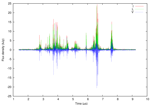
Figure 2: Example of GP detected at 8.5 GHz shown with a sampling time of 0.8 ns. The pulse originates close to the MP longitude. The solid red line indicates the total intensity (I), the dashed green line – the linear polarization (L), and the dashed blue line – the circular polarization (V).

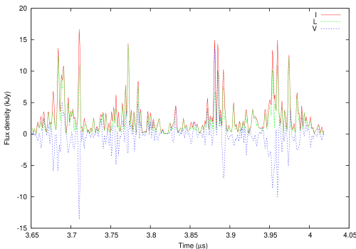
Figure 3: Zoom-in portion of the GP shown in Figure 2. The solid red line indicates the total intensity (I), the dashed green line – the linear polarization (L), and the dashed blue line – the circular polarization (V).

Figure 4: Example of GP detected at 8.5 GHz shown with a sampling time of 0.8 ns. The pulse originates at IP longitudes. The solid red line indicates the total intensity (I), the dashed green line – the linear polarization (L), and the dashed blue line – the circular polarization (V).

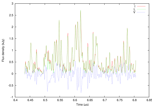
Figure 5: Zoom-in portion of the GP shown in Figure 4. The solid red line indicates the total intensity (I), the dashed green line – the linear polarization (L), and the dashed blue line – the circular polarization (V).

4.2 Shapes of single pulses

Examples of strong GP profiles at 8.5 GHz both at the longitudes of MP and IP are presented in Figs. 2–5 simultaneously in total intensity ($I$), linear ($L$), and circular ($V$) polarizations. One can see clear differences between shape and polarization of GPs originating at longitudes of MP and IP. MP giant pulses (MPGPs, Figs. 2,3) consist of several distinct groups of “microbursts” with strong unresolved “nanoshots” in every group, while IP giant pulses (IPGPs, Figs. 4,5) demonstrate only a uniform increase of noise over a certain time interval. These differences were first reported by Hankins & Eilek (2007). There is one exceptional MPGP with a smoother waveform which we discuss below in Sects. 4.3 and 4.5. The waveforms of all IPGPs are rather similar in shape, usually showing a short rise time of about $0.6\pm 0.2\leavevmode\nobreak\ \mu$s and gradual decay after maximum for about $2.5\leavevmode\nobreak\ \mu$s. In contrast, MPGPs are very different in shape.

Figure 6: Average CCFs between GP intensities detected in two polarization channels. The left panels represent MPGPs and the right panels correspond to IPGPs. Figures at the bottom show only the central part of CCFs.

MPGPs manifest a great variety of polarization properties between different isolated microbursts exhibiting strong circular polarization of both signs and strong linear polarization as well (see Fig. 3). On the other hand, all structural components of IPGPs (as in Fig. 5) have a high degree of linear polarization. The polarization properties of GPs will be discussed in more detail further in sect. 4.3. Here we are concerned only with the derivation of general parameters describing the observed pulse shapes. The traditional method is the use of an ACF calculated for the on-pulse signal (Hankins, 1972; Popov et al., 2002). However it is known that some GPs from the Crab pulsar have unresolved components (nanoshots) with a duration shorter than 0.4 ns (Hankins & Eilek, 2007). The contribution of such components to an ACF would be undistinguishable from the impact of noise, both cause a spike at zero lag of the ACF. A better alternative method is the use of the CCF between the on-pulse signals received in two polarization channels with independent receiver noise. In this case a narrow correlation spike at zero lag reflects the presence of linearly polarized unresolved components in the time structure of a signal received from a source. The average CCFs are presented in Fig. 6. The average CCF for MPGPs (Fig. 6, left) indicates the presence of several time scales from a few nanoseconds to a few microseconds, while the CCF for IPGPs (Fig. 6, right) shows only an unresolved spike at zero lag and uniform Gaussian detail with a half-width of about $0.5\leavevmode\nobreak\ \mu$s.

Does the CCF spike at zero lag contains real unresolved nanoshots, or is it purely a result of noise? The amplitude of isolated narrow pulses is very sensitive to the accuracy of the value of DM used for coherent dedispersion (Rickett, 1975). When processing with a range of assumed DM values, one may expect a rapid peaking of the zero-lag CCF spike near the correct DM in the presence of unresolved nanoshots, and the absence of such a prominent maximum if only noise is present.

We adopt a value $a_{0}=D_{\mathrm{max}}-D_{\mathrm{min}}$ as amplitude of a zero-lag spike above the broader CCF shoulders, with $D_{\mathrm{max}}$ and $D_{\mathrm{min}}$ being maximum and minimum values in a series of $D_{i}$ calculated as $D_{i}=\mathrm{CCF}_{i+1}-\mathrm{CCF}_{i}$ in the range of time lag $\pm\Delta t$ near the zero lag.

Figure 7: The dependence of the value of $a_{0}$ (see text) versus DM for MPGPs (open squares) and IPGPs (filled squares).

The dependence of $a_{0}$ versus DM for MPGPs and IPGPs is shown in Fig. 7. Open squares represent the mean values of $a_{0}$ averaged over 5 strong GPs detected at 8.5 GHz within the the MP longitude range. Closed squares represent mean values of $a_{0}$ averaged over 5 strong GPs detected at the same frequency at IP longitudes. The curve for MPGPs has a very sharp maximum at $\mathrm{DM}=56.766$ pc cm^-3, which corresponds closely to the value published in the Jodrell Bank Crab Pulsar Monthly Ephemeris (Lyne et al., 2008) for our observing epoch. The zero-lag peak of the CCF for IP data exists and has large amplitude, however no marked dependence on assumed DM is found in this case. Thus for the IP there is no evidence of large unresolved nanoshots which we might identify with individual emitters. It is interesting to note that the central CCF peak for IP data has the same amplitude as that of the extended CCF shoulders in agreement with the amplitude modulated noise (AMN) model proposed by Rickett (1975) to explain microstructure in pulsar radio emission.

4.3 Polarization of single pulses

The calibration and processing described in section 3.5 allowed us to present examples of GP profiles in Figs. 2–5 with full time resolution. They show a huge variety of polarization behavior, especially for GPs corresponding to the MP longitude (see Fig. 3), where neighboring bursts may have opposite signs of circular polarization. In an attempt to find trends in the observed parameters, particularly for the evolution of position angle (PA) of polarization, we first applied running averaging with a bin size of 80 ns to all four Stokes parameters for each GP. Examples of such smoothed GPs are shown in Fig. 8. Left and right panels of the Fig. 8 represent typical profiles of MPGP and IPGP respectively. The middle panel shows an unusual MPGP mentioned in Sect. 4.2. Fig. 8 shows the evident differences between polarization properties of MPGPs and IPGPs. An IPGP usually has a high degree of linear polarization (up to 100% at the maximum) and small variations of position angle, less than $\pm 5\degr$ peak-to-peak.

An MPGP shows a smaller degree of linear polarization (30–50%), and greater variations of PA ($\pm 20$–$40\degr$). The PA evolves smoothly within separate components, with varying sweep rates and ranges. These properties were confirmed for the majority of GPs.

All IPGPs have similar properties, with one exception which we will discuss briefly in Sect. 4.5. The PA is largely constant, and it is about the same for all IPGPs at both frequencies, 8.5 and 15.1 GHz. In contrast to that, every MPGP is different. PA values for MPGPs vary randomly from pulse to pulse, as well as within the single pulse, in the whole range of 0–$180\degr$.

As discussed in Sect. 4.2, MPGPs exhibit a great variety of shapes. They consist of several dense clusters (components) of microbursts containing strong unresolved nanoshots (Fig. 2 and left panel of Fig. 8). Within a distinct component or microburst, PA demonstrates a very regular smooth variation over a range of a few tens of degrees. The PA sweep varies strongly from one component to another and may also have an opposite sign in neighboring microbursts.

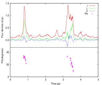
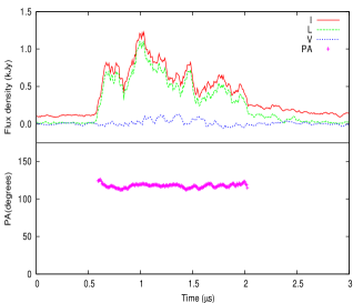
Figure 8: Smoothed profiles and position angle (PA) evolution for selected MPGP (left), peculiar MPGP (middle, see Sect. 4.5), and IPGP (right). The IPGP shown was detected at 15.1 GHz, while the MPGPs were found at 8.5 GHz. PA is in degrees (Y-axis), and intensity is in kJy. The solid red line indicates the total intensity, the dashed green line – the linear polarization, the dashed blue line – the circular polarization, and black crosses – the PA variation.

The MPGP shown in the middle panel of the Fig. 8 has a very smooth, wide waveform without any clustering of microbursts, which is untypical for MPGPs. Perhaps it represents a different, uncommon category of MPGPs, therefore we discuss this pulse separately in Sect. 4.5. Regular PA variation is seen throughout the pulse duration rotating smoothly from $118\degr$ to $75\degr$. Another remarkable feature of this particular GP is a surprising coincidence of its intensity in linear and circular polarizations.

Smooth regular variations of PA seen in MPGPs are similar to those typical of integrated profiles of many pulsars, which show a classical S-shape swing (see, e.g., von Hoensbroech & Xilouris, 1997). It is tempting to apply the geometric rotating vector model (RVM, Radhakrishnan & Cooke, 1969), commonly adopted in studying polar cap geometry, to explain PA evolution in MPGPs. This is considered in Sect. 5.

4.3.1 Polarization of nanoshots

Further, we tried to obtain the average polarization profile of isolated unresolved spikes (nanoshots) present in GPs. All such spikes with intensity above a given threshold were aligned in time by their maxima and added together. To avoid effects of variations of PA with GP duration, the intensity in linear polarization was averaged using the magnitude of $L=\sqrt{Q^{2}+U^{2}}$. Also, the signal was smoothed by 5 samples to reduce noise fluctuations.

Typical GPs contained from several dozens up to hundreds of strong isolated spikes. Examples of polarization profiles of such spikes are presented in Fig. 9.

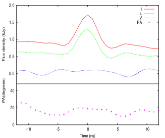
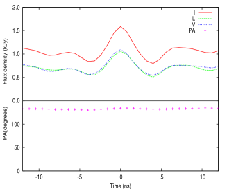
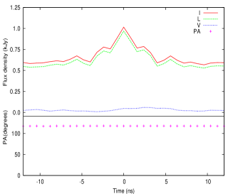
Figure 9: Average profiles and position angle (PA) evolution of strong isolated spikes which are taken from the corresponding GP from Fig. 8. PA is in degrees (Y-axis), and intensity is in kJy. The solid red line indicates the total intensity, the dashed green line – the linear polarization, the dashed blue line – the circular polarization, and black crosses – the PA variation.

We hoped to find a regular behavior of PA or circular polarization ($V$) through the average profile of a strong isolated emission spikes. However, no general dependence for all GPs was found, not even for neighboring subsets of GPs. Nevertheless, Figs. 8 and 9 present examples of typical MPGPs (left and the middle panels), and IPGPs (right panel). The average profile for spikes belonging to MPGPs (Fig. 9, left) indicates that these nanoshots are truly isolated (no other components are seen within at least ten nanoseconds). Such nanoshots have an approximately equal degree of circular and linear polarization. However on average their Stokes parameter $V$ is close to zero because of the nearly equal contributions from RHC and LHC components. The average position angle does not show any regular variation within the duration of a nanoshot.

The central panels in Figs. 8 and 9 represent polarization properties of the peculiar MPGP. The profile of average spikes also reveals a remarkable feature of this GP: the degree of linear polarization is equal to the degree of circular polarization, and the majority of spikes have circular polarization of the same sign (RHC). In fact, values of $L$ and $V$ stay astonishingly close together over the whole pulse duration. They also evolve together in the average profile of outstanding spikes (see Fig. 9). This average profile indicates the presence of close satellites near the majority of spikes with similar polarization properties. The PA varies slightly.

The polarization properties displayed in the right panels of Figs. 8 and 9 correspond to the IPGPs. A high degree of linear polarization is evident in both the smoothed pulse profile and in the average profile of spikes. This profile contains of many small spikes merged together. Also, the profile confirms a constancy of PA for IPGP.

4.3.2 Polarization statistics of nanoshots

Some statistical properties of GP polarization are presented in Fig. 10. Linear and circular polarizations, and position angle were calculated at the point of maximum total intensity $I$ for every spike above a given threshold in $I$ ($10\sigma$ in signal smoothed by 5 samples). There are 3250, 311, 720, and 2360 measurements for MPGPs and IPGPs at 8.5 GHz, and MPGPs and IPGPs at 15.1 GHz, respectively.

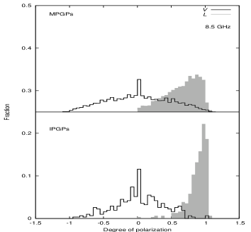
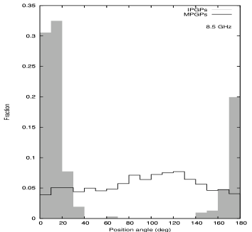
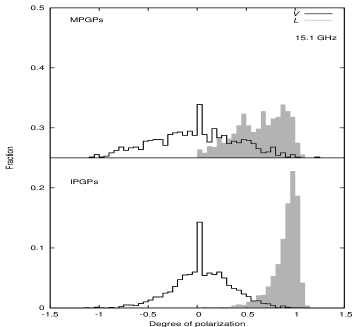
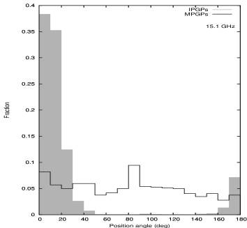
Figure 10: Histograms of degree of polarization (left panels) and position angle of linear polarization (right panels) for individual isolated strong spikes of radio emission constituting every GP. Top panels correspond to GPs detected at 8.5 GHz, and bottom panels – to GPs at 15.1 GHz. For histograms of degree of polarization, open histograms represent the circular polarization, and filled histograms – linear polarization.

One can see that the polarization properties of spikes which constitute GP radio emission are nearly identical at both 8.5 and 15.1 GHz. MPGPs demonstrate a rather broad distribution over the degree of circular and linear polarization, and the PA of linear polarization shows a uniform distribution. The distribution of the degree of polarization of IPGP spikes is narrower with a greater portion of events having a high degree of linear polarization and PA is concentrated in a restricted range of values between $-10\degr$ and $+20\degr$. It seems that there is also a distinct population of short spikes with pure linear polarization, which produce a narrow maximum at $V=0$ in the distributions over the degree of circular polarization. The observed degree of linear and circular polarizations is quite different from those observed for the GPs from the millisecond pulsar B1937+21 (Kondratiev et al., 2007), where the majority of GPs were either highly circularly or linearly polarized, but the degree of linear polarization did not exceed 0.6.

4.4 Spectra of single pulses

To obtain dynamic spectra of the GPs we calculated the detected signal in narrow bands consisting of 8192 samples corresponding to 9.765 MHz channel bandwidth after applying phase corrections to the total spectrum. There are 44 and 55 such narrow bands in the dynamic spectra at 8.5 and 15.1 GHz, correspondingly, with the sampling time being equal to 51.2 ns. Examples of dynamic spectra for selected GPs are shown in Fig. 11.

Hankins & Eilek (2007) found striking differences in the radio spectra of both MPGPs and IPGPs. IPGPs have emission bands proportionally spaced in frequency with $\Delta\nu/\nu\approx 0.06$, while MPGPs are characterized by broad-band spectra which smoothly fill the entire observing bandwidth. Our observations confirm the presence of emission bands in IPGPs radio spectra at both 8.5 and 15.1 GHz (see Fig. 11, bottom-left). The total bandwidth we used (about 0.5 GHz) does not allow us to measure the spacing between emission bands, since the expected values are 0.5 and 0.9 GHz at 8.5 and 15.1 GHz, respectively. The two emission regions seen in the bottom-left panel of Fig. 11 do not represent separate emission bands but constitute the internal structure of an emission band typical for IPGPs, as was demonstrated by Hankins & Eilek (2007).

We attempted to estimate the characteristic bandwidth of such structures by analyzing the 2-D CCF between dynamic spectra for RHC and LHC polarization channels. CCFs instead of ACFs were used in order to reduce the contribution from the receiver noise at the ACF origin. Because of the large degree of linear polarization such CCFs have a good signal-to-noise ratio, particularly for IPGPs. Although the receiver noise was suppressed, the effect of correlated noise from the strong background linear polarization remains. The resulting average CCFs are displayed in Fig. 12. and show clear differences between IPGP and MPGP CCFs. There are broad components in the CCFs for the IPGP for which Gaussians with half-widths of 40 and 60 MHz can be fitted for 8.5 and 15.1 GHz respectively. The observed increase in bandwidth is roughly proportional to frequency similar to the effect seen in the separation between emission bands (Hankins & Eilek, 2007). Narrow repetitive features in the frequency direction with a period of about 40 MHz are evident in the CCFs of MPGPs at 8.5 and 15.1 GHz respectively. The pattern is stronger for MPGPs at 15.1 GHz. In Fig. 13 we present the cuts of averaged CCFs for MPGPs and IPGPs along the frequency axis at zero time lag which shows the feature quite clearly and enables the determination of their separation. The features are too strong to be of a background or instrumental origin and if they were, they should also be visible in the background of the IPGP and be independent of the time lag which they are not, as seen in Fig. 12 for 15.1 GHz MPGP. Closer inspection of the MPGP dynamic spectra (top of Fig. 11) reveals that there are also strong repetitive features in frequency when GP intensities are low. This is not the case for the IPGPs. Broad features cannot be distinguished as they are comparable to the total receiver bandwidths (185 and 235 MHz at 8.5 and 15.1 GHz, respectively).

4.5 Peculiar giant pulses

While in the previous sections we emphasized the differences in properties of GPs belonging to MP and IP longitudes, a few examples of peculiar giant pulses were seen which violate general rules. One example is shown in Fig. 8, middle. For future reference we designate this pulse as GP 639 using the fractional part of seconds in its arrival time as a label. Seen at the MPGP longitude at 8.5 GHz, GP 639 has a smooth shape and high degree of linear and circular polarization otherwise typical of IPGPs. Moreover, the degrees of linear and circular polarization are astonishingly similar in value over the whole profile. These parameters are also similar for the average profile of individual spikes constituting this GP (see Fig. 9, middle). It is unlikely that such combination of a polarization properties was produced by chance. GP 639 has also a distinct appearance in the dynamic spectrum with an unusual curvature at the low frequency part of the band (Fig. 11, upper-right). Such a curvature in dynamic spectra was found by Hankins & Eilek (2007) for IPGPs.

Another example of a peculiar GP is presented by GP 594 detected at 8.5 GHz at the IP longitude (Fig. 11, bottom-right). This pulse does not manifest any emission bands in its dynamic spectrum in contrast to the majority of IPGPs (see bottom-left and bottom-right panels of Fig. 11 for comparison). It is interesting to note that the arrival longitude of GP 594 corresponds to that of IPs seen in the frequency range below 4 GHz. Thus, it appears that this pulse did not undergo any longitude shift and modulation of its radio spectrum.

5 Discussion

In our study we have found a very sharp difference in properties of MPGPs and IPGPs which are summarized below in Sect. 6. During our observations at both 8.5 and 15.1 GHz no GPs at the longitudes of HFCs were found. However, Jessner et al. (2005) reported detecting GPs in all phases of normal radio emission at the similar frequency of 8.35 GHz. In their experiment they

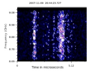
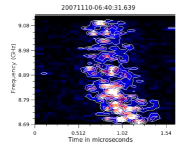
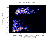
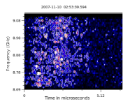
Figure 11: Dynamic spectra of selected GPs. Left plots show the typical examples of dynamic spectra for MPGPs (top) and IPGPs (bottom). Right plots show the peculiar GPs detected at 8.5 GHz at the longitude of MP (top, GP 639) and IP (bottom, GP 594).

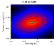
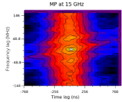
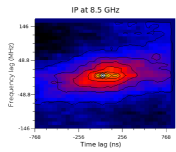
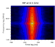
Figure 12: Average 2-D CCFs between dynamic spectra for RHC and LHC polarization channels at the frequency of 15.1 GHz (top) and 8.5 GHz (bottom) for both IPGPs (left) and MPGPs (right). Contour levels are equidistant in steps of 10% of the maxima given in fig. 13.

used the standard Effelsberg Pulsar Observation System (EPOS) and a similar ultra-high time resolution oscilloscope (Le Croy LC584AL). About 5% of the GPs detected by EPOS occurred at phases corresponding to the HFCs, the GPs themselves were usually quite weak and only very few strong ones were detected. The pulse phases of the oscilloscope data could not be determined with sufficient accuracy to allow the identification of GPs occurring at HFC pulse phases. In the 2007 experiment we detected 29 GPs at 8.5 GHz so that the predicted probability of detecting at any GPs in the HFC phase range is very low. As most GPs are below the trigger threshold of the high resolution equipment, the absence of detected GPs in the HFC range at 8.5 GHz is not unexpected. The problem is further aggravated at 15.1 GHz, where integrated profiles do not show any HFC emission and GP emission probabilities of the Crab pulsar seem to follow the integrated pulse profile.

5.1 Rotation of polarization plane

As was mentioned in Sect. 4.3, distinct microbursts of MPGPs have position angles showing a classical smooth sweep that is very similar to that observed for integrated profiles of normal radio pulsars. This “text-book” S-sweep is well-described by a geometric rotating vector model (RVM, Radhakrishnan & Cooke, 1969). Is it possible to explain apparent PA change in MPGPs with the RVM model? Formal fitting gives an improbably small value of the impact parameter of $0.1$–$20\arcsec$ from the magnetic axis. This corresponds to the linear distance of just 1–20 mm near the star’s surface and 1–100 m at the light cylinder. This is a natural consequence of the fast PA variations, typically of $\sim 40$–$60\degr$ over about 500 ns, sometimes even faster. The strongest of the detected pulses observed at 8.5 GHz, consisting of two close very narrow spikes, shows a $20\degr$ smooth PA change over only 4 ns!

One has to note, however, that for a rapidly rotating pulsar the magnetosphere differs greatly from that of a slowly rotating dipole anchored to a non-compact body. For a neutron star, any emission originating at heights of less than $1R_{\mathrm{NS}}$ will be affected by the additional curvature of field lines caused by the Lens-Thirring effect. A description of the field configuration near the surface of the star was given by Muslimov & Tsygan (1992). The simple RVM fails for another reason within the pulsar magnetosphere. It had been shown by Dyks & Rudak (2003) as well as by Wang et al. (2006) that aberration and retardation distort the magnetic field lines and cause significant modifications to the PA curve for real pulsars. These effects need to be considered in any attempts to locate the GP within the magnetosphere. The fact that MPGPs and IPGPs have such different characteristics may point to propagation effects within the pulsar magnetosphere, where different ray paths will affect the signals differently, leading to additional scintillation and polarization effects.

However there are two simple heuristic ways to solve the problem in the frame of RVM. First, let us suppose that the local magnetic field at the polar cap near the star’s surface has a structure consisting of a number of narrow field tubes similar to that observed in solar spots. In this case the impact parameter is the distance from the center of the local flux tube. Individual microbursts are related to different tubes, the impact parameter is small but distinct for different microbursts. It is expected that the polar cap current will break up into individual filaments carrying currents of order $1.7\times 10^{4}\times\gamma^{3}$ A, forming small flux tubes as a consequence. The details of the radio emission from such flux tubes are the subject of a forthcoming paper.

The second possibility is that the PA sweep is related, not to the relatively slow rotation of the neutron star but to rapid movement of the GP emitter across the polar cap with the velocity of the order of the speed of light. The emitter then crosses a polar cap in different directions at different distances from the magnetic axis. However, the exact nature of such an emitter is unknown at present.

5.2 Emission mechanism

Though several hypotheses and models have been put forward to explain the GP phenomenon, none of them can fully quantitatively address all the observed properties of GPs. A number of attempts have been undertaken to implement plasma mechanisms for generation of GPs (Petrova, 2006; Weatherall, 1998; Lyutikov, 2007; Istomin, 2004). However, Hankins et al. (2003) pointed out that the volume density of energy of GP emission is of the same order as the volume density of plasma energy and sometimes even exceeds it for the strongest GPs with peak flux densities of several million janskys, as recently reported by Soglasnov (2007) and Hankins & Eilek (2007). Moreover, a very high field strength of electromagnetic waves does affect the interaction between the wave and particles (Soglasnov, 2007) significantly, so that the mechanisms of linear plasma theory are no longer applicable.

It is very attractive to suppose that GPs are generated directly by a polar cap discharge when cascade pair creation leads to a rapidly increasing volume charge and current. Microbursts observed in MPGPs could be identified with sparks in the polar gap. IPGPs at high frequencies seem to be a rather stable phenomenon, and they can be described as “well-mixed emission” probably as a result of some scattering process (e.g. by inverse Compton scattering as suggested by Petrova, 2009). An alternative explanation of GP emission mechanism will be discussed in detail by Soglasnov (2010). Here we sketch only a very preliminary scenario of GP generation.

Originally GPs are created as a direct consequence of the polar cap discharge. A part of the energy of the GP is spent on particle acceleration. Because of the steep power-law radio spectrum, only the strongest GPs are detectable at high frequencies, while weak ones (which mainly form an average profile) disappear completely. This explains that in the case of MPGPs we see the faint but true original MP in their average profile at high frequencies, as well as strong but rare GPs at corresponding longitudes of the MP.

The interpulse is weaker since it vanishes earlier at lower radio frequencies than the MP. What we see at higher frequencies is not the “true” IPGP, but the emission of relativistic particles accelerated by the original IPGP.

The repetitive frequency pattern that we observed can be the result of a diffraction effect, either from differing propagation paths in the pulsar magnetosphere or from the shape and structure of the coherent IP emission zone itself. The 40 MHz separation seen in the dynamic spectra of MPGPs would then correspond to a path difference of 7.5 m. The fact that the dynamic spectra show regular but rather strong and narrow spikes of a width of less than 10 MHz over a weaker background can be interpreted as the emission from a succession of more than four very narrow discharge zones (unresolved width $<{c\over\rm 500\leavevmode\nobreak\ MHz}=\rm 0.6\leavevmode\nobreak\ m$) along the line of sight. In that case, one would also expect these features to be more clearly visible at higher frequencies, because at higher frequencies the phase of the radio emission from an individual narrow discharge zone will be more clearly defined, giving stronger interference patterns. Additional support for the existence of nanoshot discharges can be obtained from high frequency observations of ordinary pulsars. The typical shape of their spectra may be interpreted as being caused by a superposition of radiation from such nanoshot discharge regions (Loehmer et al., 2008).

Figure 13: Frequency cuts of 2-D CCFs from the Fig. 12 between dynamic spectra at the frequency of 8.5 GHz (open squares) and 15.1 GHz (filled squares) for IPGPs (top) and MPGPs (bottom).

6 Summary

A very striking difference in properties of MPGPs and IPGPs was revealed in our study.

6.1 IPGPs

1. Waveform: IPGPs are always smooth in shape and typically asymmetric, with a rather sharp leading edge with a rise time of $0.6\pm 0.2\leavevmode\nobreak\ \mu$s and gradual decay of about $2.5\leavevmode\nobreak\ \mu$s at the trailing edge.

2. Internal emission structure: IPGPs are filled with pure noise well described by the AMN model (Rickett, 1975).

3. Polarization: IPGPs exhibit a high degree of linear polarization with essentially a constant PA, restricted in the range of $\pm 5\degr$, similar at both 8.5 and 15.1 GHz.

4. Spectra: Radio spectra of IPGPs consist of emission bands at 8.5 and 15.1 GHz as was first reported by Hankins & Eilek (2007). The half-width of the emission bands was found to be equal to 40 and 60 MHz for 8.5 and 15.1 GHz, respectively.

6.2 MPGPs

1. Waveform: MPGPs demonstrate a large variety of shapes containing one or several microbursts of emission with a duration of less than a microsecond. The bursts can occur intermittently at random time intervals of several microseconds duration. The total time envelope of a given GP can extend over hundreds of microseconds. Microbursts can often contain isolated or overlapping unresolved nanoshots of great intensity.

2. Internal emission structure: MPGPs are composed of distinct unresolved small spikes.

3. Polarization: MPGPs show a significant diversity of polarization parameters, with linearly and circularly polarized spikes being present in roughly equal proportions. The distribution of linearly polarized spikes (nanoshots) over PA looks uniform in the whole range of 0–$180\degr$. In the case of well-separated microbursts, PA demonstrates a rapid but smooth regular variation inside a microburst, very similar to that observed for integrated profiles of many pulsars.

4. Spectra: Dynamic spectra of MPGPs are broad-band, filling the entire observing bandwidth of 0.5 GHz. MPGPs show additional regular spiky frequency patterns with a separation of about 40 MHz in their dynamic spectra. These also show up in CCF between LHC and RHC polarization signals.

Such sharp contrasts between MPGPs and IPGPs are not observed at lower frequencies. On the other hand it seems hardly probable that the emission mechanism of GPs is very different at high and low frequencies, hence the reason for the widely different GP characteristics at different pulse phases remains unknown.