Free energy cascade in gyrokinetic turbulence

Abstract

In gyrokinetic theory, the quadratic nonlinearity is known to play an important role in the dynamics by redistributing (in a conservative fashion) the free energy between the various active scales. In the present study, the free energy transfer is analyzed for the case of ion temperature gradient driven turbulence. It is shown that it shares many properties with the energy transfer in fluid turbulence. In particular, one finds a forward (from large to small scales), extremely local, and self-similar cascade of free energy in the plane perpendicular to the background magnetic field. These findings shed light on some fundamental properties of plasma turbulence, and encourage the development of large eddy simulation techniques for gyrokinetics.

Fully developed turbulence is fundamentally linked to a conservative transfer of (free) energy in wavenumber space from drive to dissipation scales K41 . While the respective cascade dynamics for simple fluids (described by the Navier-Stokes equation) has been the subject of countless studies and is fairly well understood, the situation is quite different for turbulent plasmas, both at large scales (compared to the gyroradii of the particles) – described in the context of magnetohydrodynamics – and, in particular, at small scales – described by the gyrokinetic equations Brizard:2007p478 . The latter case, in which one deals with a gyrocenter distribution function in three spatial dimensions as well as two velocity space dimensions (the third velocity space coordinate can be removed analytically in a low-frequency ordering), shall be the focus of the present work.

In three-dimensional Navier-Stokes turbulence, the kinetic energy is conserved by the convective nonlinearity. It is usually assumed to be injected into the system at the largest scales through mechanical forcing, and to be dissipated at the smallest scales by viscous effects. The role of the nonlinearity is then to transfer the kinetic energy from the large scales to the small ones in what is usually referred to as a cascade process. In the gyrokinetic formalism, on the other hand, the free energy acts as the quadratic conserved quantity (see, e.g., Ref. 0741-3335-50-12-124024 and various references therein). It is usually injected into the system at large scales via the background density and temperature gradients, and expected to be dissipated at small (space and/or velocity space) scales. It is anticipated that one role of the nonlinear term in gyrokinetic turbulence is to transfer the free energy from the largest perpendicular scales to the smallest ones howes ; tatsuno ; 2010arXiv1003.3933T , but a definitive investigation of the free energy transfer dynamics in a self-driven, three-dimensional system (which is the standard case for magnetically confined plasmas) is still lacking and shall be provided for the first time in the present Letter.

Our study is based on numerical solutions of the nonlinear gyrokinetic equations obtained by means of the Gene code jenko:1904 ; dannert:072309 ; Merz . Although Gene is able to treat an arbitrary number of fully gyrokinetic particle species as well as general toroidal geometry, magnetic field fluctuations, and collisions, these features shall not be used here. Instead, we will focus on the reduced problem of a single ion species, adiabatic electrons, electrostatic fluctuations, and a large aspect-ratio, circular cross-section model equilibrium. For this simplified case, the respective (appropriately normalized) equations read (for details, see Ref. Merz ):

$$\frac{\partial f_{j}}{\partial t}+\Big{[}\omega_{n_{j}}+\left(v_{\parallel}^{2}+\mu B_{0}-\frac{3}{2}\right)\omega_{T_{j}}\Big{]}F_{0j}\frac{\partial\bar{\phi_{1}}}{\partial y}$$

$$+\frac{T_{0j}(2v_{\parallel}^{2}+\mu B_{0})}{q_{j}B_{0}}\left(\mathcal{K}_{x}\frac{\partial h_{j}}{\partial x}+\mathcal{K}_{y}\frac{\partial h_{j}}{\partial y}\right)$$

$$+\left[\bar{\phi_{1}},h_{j}\right]_{xy}+\frac{v_{Tj}}{2}\left[v_{\parallel}^{2}+\mu B_{0},h_{j}\right]_{zv_{\parallel}}=0\,.$$ (1)

Here, the total distribution function $F_{j}$ of species $j$ is split into a Maxwellian part $F_{0j}=\pi^{-3/2}e^{-({v_{\parallel}}^{2}+\mu B_{0})}$ and a perturbed part $f_{j}$, and the nonadiabatic part of $f_{j}$ is given by $h_{j}=f_{j}+(q_{j}\bar{\phi_{1}}/T_{0j})\,F_{0j}$ where $\overline{{\phi}}_{1}$ is the gyro-averaged electrostatic potential. $h_{j}$ and $f_{j}$ depend on the gyrocenter position ${\bf r}=(x,y,z)$, the parallel velocity $v_{\parallel}$, the magnetic moment $\mu$, and the time $t$. As indicated already above, all simulations in this paper are performed in $\hat{s}-\alpha$ geometry s-a-model with $\alpha=0$, for which the curvature terms are given by $\mathcal{K}_{x}=-2\sin z$ and $\mathcal{K}_{y}=-2(\cos z+\hat{s}z\sin z)$. Furthermore, $v_{Tj}=(2T_{j0}/m_{j})^{1/2}$ is the thermal velocity, $\omega_{n_{j}}=-R\,\partial\log n_{0j}/\partial x$ and $\omega_{T_{j}}=-R\,\partial\log T_{0j}/\partial x$ are the normalized background density and temperature gradients, $m_{j}$ and $q_{j}$ are the mass and charge of species $j$. The equilibrium magnetic field is taken to be $B=B_{0}\,B_{\rm ref}$ where $B_{\rm ref}$ is the reference magnetic field on the magnetic axis. Finally, the Poisson brackets are defined by

$$\left[f,g\right]_{ab}=\frac{\partial f}{\partial a}\frac{\partial g}{\partial b}-\frac{\partial f}{\partial b}\frac{\partial g}{\partial a}\,.$$ (2)

Note that in Eq. (1), the second term is responsible for the injection of free energy into the system. The third through fifth terms are, respectively, the curvature, nonlinear, and parallel terms, none of which acts as a source or sink of free energy. Since the simulations presented below are done without collision operator, the numerical scheme used in Gene is not dissipative, and a statistical steady state cannot be reached without some form of dissipation krommes:3211 . Here, hyperdiffusion terms $\mathcal{D}_{z}$ and $\mathcal{D}_{v_{\parallel}}$ are added to dissipate fine-scale fluctuations in $z$ and $v_{\parallel}$ (for details, see Ref. Pueschel ).

Eq. (1) is complemented by the gyrokinetic Poisson equation which is used to determine the self-consistent electrostatic potential:

$$\sum_{j}\frac{q_{j}^{2}n_{0j}}{T_{0j}}\left[1-\Gamma_{0}(b_{j})\right]{\phi}_{1}=\hskip 42.67912pt\$$

$$\ \hskip 42.67912pt\sum_{j}n_{0j}\pi q_{j}B_{0}\int J_{0}(\lambda_{j})f_{j}\,dv_{\parallel}d\mu\,.$$ (3)

Here, $J_{0}$ is the Bessel function and $\Gamma_{0}(b_{j})=e^{-b_{j}}I_{0}(b_{j})$ with the modified Bessel function $I_{0}$. The (dimensionless) arguments $b_{j}$ and $\lambda_{j}$ are defined, respectively, as

$$b_{j}=\frac{v_{T_{j}}^{2}}{2\Omega_{j}^{2}}k_{\perp}^{2}\,,\quad\lambda_{j}=\frac{v_{Tj}}{\Omega_{j}}(\mu B_{0})^{1/2}k_{\perp}$$ (4)

where $\Omega_{j}=(q_{j}B_{0})/(m_{j}c)$ and $k_{\perp}$ is the perpendicular wave number.

In the absence of drive and dissipation, the gyrokinetic equations, Eqs. (1) and (3), are known to conserve the free energy $\cal E$ (see, e.g., Refs. 0741-3335-50-12-124024 ; 2010arXiv1003.3933T ) which is usually split into two quadratic parts according to ${\cal E}={\cal E}_{f}+{\cal E}_{\phi}$ with

$$\mathcal{E}_{f}=\sum_{j}\int d\Lambda\,\frac{T_{0j}}{F_{0j}}\frac{f_{j}^{2}}{2}\,,\quad\mathcal{E}_{\phi}=\sum_{j}\int d\Lambda\,q_{j}\frac{\bar{\phi_{1}}f_{j}}{2}\,.$$ (5)

Here, $\int d\Lambda=\int d^{3}x\int\pi B_{0}n_{0j}\,dv_{\parallel}d\mu$ denotes phase-space integration. The evolution equation for the free energy is given by

$$\frac{\partial\mathcal{E}}{\partial t}=\sum_{j}\int d{\Lambda}\frac{T_{0j}}{F_{0j}}h_{j}\frac{\partial f_{j}}{\partial t}=\mathcal{G}-\mathcal{D}$$ (6)

in terms of the source term

$$\mathcal{G}= -\sum_{j}\int d{\Lambda}\frac{T_{0j}}{F_{0j}}h_{j}$$

$$\cdot\Big{[}\omega_{n}+\left(v_{\parallel}^{2}+\mu B_{0}-\frac{3}{2}\right)\omega_{Tj}\Big{]}F_{0j}\frac{\partial\bar{\phi_{1}}}{\partial y}$$ (7)

and the (positive definite) dissipative term

$$\mathcal{D}=-\sum_{j}\int d{\Lambda}\frac{T_{0j}}{F_{0j}}h_{j}\left(\mathcal{D}_{z}f_{j}+\mathcal{D}_{v_{\parallel}}f_{j}\right)\,.$$ (8)

The quantity $\cal E$ plays the same role in gyrokinetic turbulence as the kinetic energy in fluid turbulence 0741-3335-50-12-124024 .

The transfer of free energy between different modes in the saturated turbulent state is induced by the nonlinear term. Although it does not affect the global value of the free energy (numerically, this is satisfied in Gene up to machine precision), it can change, e.g., the value of this quantity associated with particular perpendicular wavenumbers. Following the procedure used for studying energy transfer in Navier-Stokes and in MHD turbulence Debliquy:2005p204 ; PhysRevE.72.046301 ; PhysRevE.72.046302 ; Carati:2006p213 , we decompose the perpendicular wavevector plane into domains and measure the free energy transfer between these domains. The set of domains $\{d_{\ell}\}$ is assumed to be a partition (no intersection between the domains and all domains together cover the entire plane). The distribution function and electrostatic potential can then be written as a sum over all contributions for which the perpendicular wavevectors lie in the domain $d_{\ell}$. As a consequence of the Parseval theorem, the free energy can also be split into parts which are associated to the domains $d_{\ell}$:

$${\cal E}=\sum_{\ell}{\cal E}^{\ell}=\sum_{\ell}{\cal E}_{f}^{\ell}+\sum_{\ell}{\cal E}_{\phi}^{\ell}\,.$$ (9)

In the problem considered hereafter, both the entropy and electrostatic contributions to the free energy are conserved separately by the nonlinearity ${\cal N}$. It is thus legitimate to consider the entropy conservation independently from the conservation of the electrostatic energy. The evolution of ${\cal E}_{f}^{\ell}$ due to the nonlinear term can be expressed as

$$\frac{\partial\mathcal{E}_{f}^{\ell}}{\partial t}\Big{|}_{\mathcal{N}}=\sum_{j}\int d\Lambda\frac{T_{0j}}{F_{0j}}f_{j}^{\ell}\frac{\partial f_{j}}{\partial t}\Big{|}_{\mathcal{N}}$$ (10)

where we have used the property $\int d\Lambda f_{j}^{\ell}f_{j}^{\ell}=\int d\Lambda f_{j}^{\ell}f_{j}$ which is easily proven and expresses the fact that the contributions $f_{j}^{\ell}$ are orthogonal “vectors” if their scalar product is defined as the integration over $\Lambda$. Introducing the explicit form of the nonlinearity, one obtains

$$\frac{\partial\mathcal{E}_{f}^{\ell}}{\partial t}\Big{|}_{\mathcal{N}}=\sum_{j}\int d\Lambda\frac{T_{0j}}{F_{0j}}f_{j}^{\ell}\left[\bar{\phi}_{1},f_{j}\right]_{xy}=\sum_{\ell_{1},\ell_{2}}T^{\ell;\ell_{1},\ell_{2}}$$ (11)

where the three-domain interaction terms are defined as

$$T_{f}^{\ell;\ell_{1},\ell_{2}}=\sum_{j}\int d\Lambda\frac{T_{0j}}{F_{0j}}f_{j}^{\ell}\left[\bar{\phi}_{1}^{\ell_{1}},f_{j}^{\ell_{2}}\right]_{xy}\,.$$ (12)

Eq. (11) shows that the evolution of the entropy associated to the domain $d_{\ell}$ is the sum of triple interactions between wave vectors associated to the domains $d_{\ell}$, $d_{\ell_{1}}$ and $d_{\ell_{2}}$. This is not a surprise since, like in the Navier-Stokes equation, the quadratic nonlinearity in the gyrokinetic equation is responsible for triadic interactions between the Fourier modes. Proposing a clean definition of the energy transfer between two domains might thus be problematic in such a picture. However, considering the structure of these three-domain interaction terms, the following two-domain interaction terms is a natural quantity to investigate:

$$T_{f}^{\ell,\ell^{\prime}}=\sum_{\ell_{1}}T_{f}^{\ell;\ell_{1},\ell^{\prime}}=\sum_{j}\int d\Lambda\frac{T_{0j}}{F_{0j}}f_{j}^{\ell}\left[\bar{\phi}_{1},f_{j}^{\ell^{\prime}}\right]_{xy}\,.$$ (13)

These two-domain interaction terms will be interpreted as the energy transfers between the domains $d_{\ell}$ and $d_{\ell^{\prime}}$, even if the redistribution of the free energy between the different domains by the nonlinear term cannot be fully understood without considering triadic interactions. As a consequence of the Poisson bracket structure, it is easy to show that $T_{f}^{\ell,\ell^{\prime}}=-T_{f}^{\ell^{\prime},\ell}$, which reinforces the interpretation in terms of free energy exchange. Indeed, if the domain $d_{\ell}$ is considered to receive a certain amount of free energy per unit of time $T_{f}^{\ell,\ell^{\prime}}$ from the domain $d_{\ell^{\prime}}$, then the domain $d_{\ell^{\prime}}$ is seen as loosing exactly the same amount of free energy per unit of time in profit of the domain $d_{\ell}$. The same approach can be used to define three-domain and two-domain interaction terms for the electrostatic part of the free energy with the following definitions:

$$T_{\phi}^{\ell;\ell_{1},\ell_{2}}=\sum_{j}\int d\Lambda\bar{\phi}_{1}^{\ell}\left[\bar{\phi}_{1}^{\ell_{2}},f_{j}^{\ell_{1}}\right]_{xy}\,,$$ (14)

$$T_{\phi}^{\ell,\ell^{\prime}}=\sum_{\ell_{1}}T_{\phi}^{\ell;\ell_{1},\ell^{\prime}}=\sum_{j}\int d\Lambda\bar{\phi}_{1}^{\ell}\left[\bar{\phi}_{1}^{\ell^{\prime}},f_{j}\right]_{xy}\,.$$ (15)

The complete dynamical equation for $\mathcal{E}^{\ell}$ then reads

$$\frac{\partial\mathcal{E}^{\ell}}{\partial t}=\sum_{\ell^{\prime}}T_{f}^{\ell,\ell^{\prime}}+\sum_{\ell^{\prime}}T_{\phi}^{\ell,\ell^{\prime}}+\mathcal{G}^{\ell}-\mathcal{D}^{\ell}$$ (16)

where the source and dissipation terms, $\mathcal{G}^{\ell}$ and $\mathcal{D}^{\ell}$, are given, respectively, by Eqs. (7) and (8), using $h_{j}^{\ell}$, $f_{j}^{\ell}$, and $\bar{\phi}_{1}^{\ell}$.

The free energy transfer terms defined above are now evaluated from a numerical simulation using Gene. The physical parameters employed in this context correspond to a widely used standard case of collisionless ion temperature gradient (ITG) turbulence known as the Cyclone Base Case dimits:969 . The simulation domain is about 125 ion gyroradii wide in the perpendicular directions, and $256\times 64\times 64\times 32\times 8$ grid points are used in $(x,y,z,v_{\parallel},\mu)$ space. For further analysis, the perpendicular wavevector plane is divided into shells $d_{\ell}=\{\mathbf{k}_{\perp}\text{ such as }K_{\ell}<|\mathbf{k}_{\perp}|\leq K_{\ell+1}\}$ where the shell boundaries $K_{\ell}$ are chosen to grow algebraically $K_{\ell+1}=\lambda K_{\ell}$, with $\lambda=2^{1/5}$ between shell $\ell=3$ and $\ell=24$. The first shell boundaries have been chosen differently ($K_{1}=0$, $K_{2}=0.2$, $K_{3}=0.3$) in order to ensure that enough modes belong to those shells. Moreover, in order to limit the number of shells, the last shell ($\ell=25$) is wider and limited by $K_{25}=6.3$ and $K_{26}=|\mathbf{k_{\perp}}|_{\max}=14.6$.

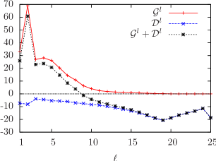
Figure 1: Shell decompositions in perpendicular wavenumber space of the drive ($\mathcal{G}^{\ell}$) and dissipation ($\mathcal{D}^{\ell}$) terms (as well as their sum) from a Gene simulation of ITG turbulence.

Fig. 1 shows the numerical results for the source and dissipation terms (averaged over time during the saturated phase of the simulation). As expected, the injection of free energy is well localized at low $k_{\perp}$ . However, as it turns out, the dissipative terms are not just active in the high $k_{\perp}$ range, but throughout the entire $k_{\perp}$ spectrum, including the drive range. An explanation of this phenomenon may be provided in terms of the nonlinear coupling to damped eigenmodes, as is discussed in Ref. Hatch10 . There is a net source of free energy up to shell $\ell=9$ and a net dissipation beyond that. The peak in the dissipation may be due to the fact that the largest shells are not complete because we are using a discretization in $k_{x}$ and $k_{y}$.

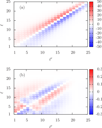
Figure 2: Shell-to-shell transfer in perpendicular wavenumber space of entropy (a) and electrostatic energy (b) from a Gene simulation of ITG turbulence.

The corresponding shell-to-shell free energy transfer terms are shown in Fig 2, and various interesting features can be observed there. First, the entropy transfer is larger than the electrostatic energy transfer by almost two orders of magnitude, thus dominating the total free energy transfer. Second, the free energy transfer is from the large scales to the small ones (as one might have expected); the transfer is systematically negative for $\ell^{\prime}>\ell$ and, due to the antisymmetry property, systematically positive otherwise. Third, the free energy transfer is very local in wavenumber space. Indeed, only values of $T_{\text{tot}}^{\ell,\ell^{\prime}}$ with $\ell$ close to $\ell^{\prime}$ are significantly different from zero. In practice, for $|\ell-\ell^{\prime}|>5$ the free energy transfers almost vanish. This corresponds to a ratio of wave numbers between the two shells of the order of two. Fourth, a limited self-similarity range can be identified for $\ell$ between 13 and 20. Indeed, in this range, the total transfers $T_{\text{tot}}^{\ell,\ell^{\prime}}$ seem to depend on $\ell-\ell^{\prime}$ only, and not on the two indices separately. Considering the limited resolution of the simulation analysed here, this property is rather unexpected. Indeed, the analysis of the source and dissipation terms (see Fig. 1) does not show the existence of a range of scales in which both these terms would be negligible. However, they are obviously sufficiently small to allow for cascade dynamics to develop (see also Ref. Hatch10 ). This is actually to be expected if the nonlinear frequencies characterizing the free energy transfer exceed the linear ones characterizing the dissipation.

Interestingly, the spectral transfer of free energy in gyrokinetic turbulence thus exhibits various similarities with respect to the kinetic energy transfer measured in fully developed Navier-Stokes turbulence, although this is not all clear a priori. In particular, there is a (strongly) local, self-similar forward cascade – despite the absence of an inertial range. Insights like these may be expected to guide the application of large-eddy simulation techniques romo84 ; agmukn01 to gyrokinetics. Here, the idea is to only retain the dynamics of the largest scales while the smallest ones are modelled. Indeed, if the smallest scales are proven to act systematically as a sink of free energy like it was the case here, it is reasonable to propose a dissipative model for these small scales and consequently reduce as much as possible the numerical resolution. On such a basis, it may well become possible to reduce the computational effort for gyrokinetic turbulence simulations by a significant amount. The present work represents a relevant step in that direction.

Acknowledgements. The authors would like to thank G. Plunk, T. Tatsuno and D. Hatch for very fruitful discussions. This work has been supported by the contract of association EURATOM - Belgian state. The content of the publication is the sole responsibility of the authors and it does not necessarily represent the views of the Commission or its services. D.C. is supported by the Fonds de la Recherche Scientifique (Belgium).

References

- (1) G. Falkovich and K. R. Sreenivasan, Physics Today 59, 43 (2006)
- (2) A. J. Brizard and T. S. Hahm, Rev. Mod. Phys. 79, 421 (2007)
- (3) A. A. Schekochihin et al., Astrophys. J. 182, 310 (2009)
- (4) G. G. Howes et al., Phys. Rev. Lett. 100, 065004 (2008)
- (5) T. Tatsuno et al., Phys. Rev. Lett. 103, 015003 (2009)
- (6) T. Tatsuno et al., arXiv:1003.3933
- (7) F. Jenko et al., Phys. Plasmas 7, 1904 (2000)
- (8) T. Dannert and F. Jenko, Phys. Plasmas 12, 072309 (2005)
- (9) F. Merz, Gyrokinetic Simulation of Multimode Plasma Turbulence. PhD thesis, Westfälische Wilhelms-Universität Münster, 2009.
- (10) J. W. Connor, R. J. Hastie, and J. B. Taylor, Phys. Rev. Lett. 40, 396 (1978)
- (11) J. A. Krommes and G. Hu, Phys. Plasmas 1, 3211 (1994)
- (12) M. J. Pueschel, T. Dannert, and F. Jenko, Comp. Phys. Comm. 181, 1428 (2010)
- (13) O. Debliquy, M. K. Verma, and D. Carati, Phys. Plasmas 12, 2309 (2005)
- (14) A. Alexakis, P. D. Mininni, and A. Pouquet, Phys. Rev. E 72, 046301 (2005)
- (15) P. D. Mininni, A. Alexakis, and A. Pouquet, Phys. Rev. E 72, 046302 (2005)
- (16) D. Carati et al., J. Turbulence 7, N51 (2006)
- (17) A. M. Dimits et al., Phys. Plasmas 7, 969 (2000)
- (18) D. R. Hatch et al., submitted for publication.
- (19) R. Rogallo and P. Moin, Annu. Rev. Fluid Mech. 16, 99 (1984)
- (20) O. Agullo et al., Phys. Plasmas 7, 3502 (2001)