Fractional relaxation and wave equations for dielectrics characterized by the Havriliak-Negami response function

Abstract

A fractional relaxation equation in dielectrics with response function of the Havriliak-Negami type is derived. An explicit expression for the fractional operator in this equation is obtained and Monte Carlo algorithm for calculation of action of this operator and is constructed. Relaxation functions calculated numerically according to this scheme coincide with analytical functions obtained earlier by other authors. The algorithm represents a numerical way of calculation in relaxation problems with arbitrary initial and boundary conditions. A fractional equation for electromagnetic waves in such dielectric media is obtained. Numerical results are in a good agreement with experimental data.

,

1 Introduction

When a step-wise electric field is applied, polarization of a material approaches its equilibrium value not instantly but after some time later. Hereditary effect of polarization is expressed through the integral relation. For electric induction in an isotropic medium, we have [Fröhlich (1958)]

$$\mathbf{D}(t)=\varepsilon_{\infty}\ \mathbf{E}(t)+\int\limits_{-\infty}^{t}\kappa(t-t^{\prime})\ \mathbf{E}(t^{\prime})dt^{\prime}.$$ (1)

Fourier transformation of the last expression gives

$$\tilde{\mathbf{D}}(\omega)=\varepsilon^{*}(\omega)\tilde{\mathbf{E}}(\omega),\quad\varepsilon^{*}(\omega)=\varepsilon_{\infty}+\tilde{\kappa}(\omega)$$

Relaxation properties of different media (dielectrics, semiconductors, ferromagnetics, and so on) are normally expressed in terms of time-domain response function $\phi(t)$ which represents the current flowing under the action of a step-function electric field, or of the frequency-dependent real and imaginary components of its Fourier transform:

$$\widetilde{\phi}(\omega)=\int\limits_{0}^{\infty}e^{-i\omega t}\phi(t)dt=\phi^{\prime}(\omega)-i\phi^{\prime\prime}(\omega).$$

The Fourier transform of the response function $\phi(t)$ is related to the frequency dependence of dielectric permittivity through the following relation

$$\tilde{\phi}(\omega)=\frac{\varepsilon^{*}(\omega)-\varepsilon_{\infty}}{\varepsilon_{s}-\varepsilon_{\infty}},\quad\tilde{\kappa}(\omega)=(\varepsilon_{s}-\varepsilon_{\infty})\tilde{\phi}(\omega).$$

Here $\varepsilon_{s}=\varepsilon^{*}(0)$ is the stationary dielectric permittivity.

The classical Debye expression (see Debye (1954)) for a system of noninteracting randomly oriented dipoles freely floating in a neutral viscous liquid is

$$\widetilde{\phi}(\omega)=\frac{1}{1+i\omega\tau},$$

where $\tau$ is the temperature-dependent relaxation time characterizing the Debye process:

$$\phi(t)=\phi(0)\exp(-t/\tau),\quad t>0.$$

The latter function obeys the simple differential equation

$$\frac{d\phi(t)}{dt}+\tau^{-1}\phi(t)=0.$$

Numerous experimental data gathered, for instance, in books (Jonscher (1977), Ramakrishnan & Lakshmi (1987)) convincingly show that this theory is not able to describe relaxation processes in solids, the relaxation behavior may deviate considerably from the exponential Debye pattern and exhibits a broad distribution of relaxation times. There exist a few other empirical response functions for solids: the Cole Cole function (Cole & Cole (1941))

$$\tilde{\phi}(\omega)=\frac{1}{1+(i\omega/\omega_{p})^{\alpha}},\qquad 0<\alpha<1,$$ (2)

the Cole-Davidson function (Davidson & Cole (1951))

$$\tilde{\phi}(\omega)=\frac{1}{(1+(i\omega/\omega_{p}))^{\beta}},\qquad 0<\beta<1,$$ (3)

and the Havriliak-Negami function (Havriliak & Negami (1966))

$$\tilde{\phi}(\omega)=\frac{1}{(1+(i\omega/\omega_{p})^{\alpha})^{\beta}},\qquad 0<\alpha,\beta<1.$$ (4)

Here $\omega_{p}$ is the peak of losses, $\alpha$ and $\beta$ are constant parameters.

In the present paper, we obtain a fractional relaxation equation in dielectrics with response function of the Havriliak-Negami type. With the help of definitions of the functional analysis we derive the explicit expression for fractional operator in this equation. Then we construct a Monte Carlo algorithm for calculation of action of this operator and of the inverse one. The algorithm represents a numerical way of calculation in relaxation problems with arbitrary initial and boundary conditions. Then, we consider propagation of electromagnetic waves in such dielectric media and discuss memory phenomenon.

2 Havriliak-Negami’s relaxation

The most general approximation for frequency dependence of response function is given by two-parameter formula proposed by Havriliak & Negami (1966). The solution of the corresponding fractional differential equation

$$\left[1+(\tau\ _{0}\textsf{D}_{t})^{\alpha}\right]^{\beta}\phi(t)=\delta(t),\qquad\tau=1/\omega_{p},$$ (5)

based on the expansion of fractional power of operator sum into infinite Newton’s series

$$\left[1+(\tau\ _{0}\textsf{D}_{t})^{\alpha}\right]^{\beta}=\sum\limits_{n=0}^{\infty}{\beta\choose n}\left(\tau\ _{0}\textsf{D}_{t}\right)^{\alpha(\beta-n)},$$

has been obtained by Novikov et al. (2005):

$$\phi(t)=-\frac{1}{\Gamma(\beta)}\sum\limits_{n=0}^{\infty}\frac{(-1)^{n}\Gamma(n+\beta)}{n!\Gamma(\alpha(n+\beta))}\left(\frac{t}{\tau}\right)^{\alpha(n+\beta)}.$$

The operator $\left[1+\omega_{p}^{-\alpha}(_{0}\textsf{D}_{t})^{\alpha}\right]^{\beta}$ can also be presented in the form (Nigmatullin & Ryabov (1997)):

$$\textsf{W}^{\alpha,\beta}_{\omega_{p}}f(t)=[1+\omega_{p}^{-\alpha}\ {}_{0}\textsf{D}_{t}^{\alpha}]^{\beta}f(t)=$$

$$\omega_{p}^{-\alpha\beta}\exp\left(-\frac{\omega_{p}^{\alpha}t}{\alpha}\ _{0}\textsf{D}^{1-\alpha}_{t}\right)\ _{0}\textsf{D}^{\alpha\beta}_{t}\exp\left(\frac{\omega_{p}^{\alpha}t}{\alpha}\ _{0}\textsf{D}^{1-\alpha}_{t}\right)f(t)$$

The HN function is considered as a general expression for the universal relaxation law (Jonscher (1996)). This universality is observed in dielectric relaxation in dipolar and nonpolar materials, conduction in hopping electronic semiconductors, conduction in ionic conductors, trapping in semiconductors, decay of delayed luminescence, surface conduction on insulators, chemical reaction kinetics, mechanical relaxation, magnetic relaxation. Despite of quite different intrinsic mechanisms, the processes manifest astonishing similarity (Jonscher, 1996). The situation seems to be similar to diffusion processes. Random movements of small pollen grain visible under a microscope, neutrons in nuclear reactors, electrons in semiconductors are quite different processes from physical point of view but they are the same process of Brownian motion from stochastic point of view. This analogy stimulates search of an appropriate stochastic model for the universal relaxation law. Investigations of such kind have been carried out in the works (Weron & Kotulski (1996), Weron (1991), Nigmatullin (1984) Nigmatullin & Ryabov (1997), Glöckle (1993), Jurlewicz & Weron (2000), Coffey et al. (2002), Déjardin (2003), Aydiner (2005)).

Weron & Jurlewicz (2005) have shown how to modify the random-walk scheme underlying the classical Debye response in order to derive the empirical Havriliak-Negami function. Moreover, they have derived formulas for simulation of random variables with probability density function, Fourier transform of which is the Havriliak-Negami function. These relations contain stable random variables.

Coffey et al. (2002) reformulated the Debye theory of dielectric relaxation of an assembly of polar molecules using a fractional noninertial Fokker Planck equation to explain anomalous dielectric relaxation.

Déjardin (2003) considered the fractional approach to the orientational motion of polar molecules acted on by an external perturbation. The problem is treated in terms of noninertial rotational diffusion (configuration space only) which leads to solving a fractional Smoluchowski equation. This model is in a good agreement with experimental data for the third-order nonlinear dielectric relaxation spectra of a ferroelectric liquid crystal.

Here with the help of relations of the functional analysis for fractional powers of operators, we derive a new numerical algorithm of solution of fractional equations corresponding to the Havriliak-Negami response. This algorithm is based on Monte Carlo simulation of one-sided stable random variables.

3 Fractional operator corresponding to the Havriliak-Negami response

Let the equi-continuous semigroup $\{T_{t};t\geq 0\}$ of $C_{0}$-class be defined on locally convex linear topological B-space $F$. The infinitesimal generating operator $A$ of the semigroup $\{T_{t}\}$ is defined as

$$Af=\lim\limits_{h\downarrow 0}\ h^{-1}(T_{h}-I)\ f$$

with domain

$$D(A)=\{f\in F;\lim\limits_{h\downarrow 0}\ h^{-1}(T_{h}-I)\ f\ \ \mbox{exists in}\ F\}.$$

According to S. Bochner and R. S. Phillips, the operators

$$\tilde{T}_{t,\alpha}\ x\equiv\tilde{T}_{t}\ x=\cases{\int\limits_{0}^{\infty}t^{-1/\alpha}g^{(\alpha)}(t^{-1/\alpha}s)\ T_{s}x\ ds,&$t>0$ ,\cr\qquad\qquad\quad x,&$t=0$\cr},$$

where $g^{(\alpha)}(t)$ is a one-sided stable density, constitute an equi-continuous semigroup of $C_{0}$-class.

The corresponding infinitesimal operators are connected through the following relation (Iosida (1980)):

$$\tilde{A}_{\alpha}\ x=-(-A)^{\alpha}x,\qquad\forall x\in D(A).$$

The infinitesimal operator $-[1+_{-\infty}\textsf{D}^{\alpha}_{t}]$ generates the semigroup

$$T_{h}=e^{-h}e^{-h_{-\infty}\textsf{D}^{\alpha}_{z}},$$

According to the Bochner-Philips relation, the semigroup generated by the infinitesimal operator $[1+_{-\infty}\textsf{D}^{\alpha}_{t}]^{\beta}$, where $\beta<1$, has the form

$$\widehat{T}_{t}\ f=\int\limits_{0}^{\infty}t^{-1/\beta}g^{(\alpha)}(t^{-1/\beta}\tau)\ \widetilde{T}_{\tau}f\ d\tau=$$

$$\int\limits_{0}^{\infty}d\tau\ e^{-\tau}\ t^{-1/\beta}g^{(\beta)}(t^{-1/\beta}\tau)\int\limits_{0}^{\infty}\tau^{-1/\alpha}g^{(\alpha)}(\tau^{-1/\alpha}u)\ T_{u}f\ du$$

Considering this integral as averaging over ensembles of stable random variables, we obtain the following relationship

$$\widehat{T}_{t}\ f=\left\langle\exp\left(-t^{1/\beta}S_{\beta}\right)f\left(z-\left[t^{1/\beta}S_{\beta}\right]^{1/\alpha}S_{\alpha}\right)\right\rangle$$

From this semigroup we can obtain the corresponding infinitesimal operator $[1+_{-\infty}\textsf{D}^{\alpha}_{t}]^{\beta}$.

To find the inverse operator

$$[1+_{-\infty}\textsf{D}^{\alpha}_{t}]^{-\beta},\qquad 0<\alpha,\beta<1,$$

we use the relation for potential operator

$$A^{-1}f=\int\limits_{0}^{\infty}T_{s}fds.$$

Consequently,

$$[1+_{-\infty}\textsf{D}^{\alpha}_{t}]^{-\beta}f=$$

$$=\left\langle\ \int\limits_{0}^{\infty}\exp\left(-t^{1/\beta}S_{\beta}\right)\ f\left(z-\left(t^{1/\beta}S_{\beta}\right)^{1/\alpha}S_{\alpha}\right)dt\right\rangle.$$

Here $S_{\alpha}$ and $S_{\beta}$ are one-sided stable random variables with characteristic exponents $0<\alpha\leq 1$ and $0<\beta\leq 1$.

Introducing exponentially distributed random variable $U$, we arrive at

$$[1+_{-\infty}\textsf{D}^{\alpha}_{t}]^{-\beta}f=\left\langle\ \int\limits_{0}^{\infty}e^{-\xi}\ f\left(z-S_{\alpha}\xi^{1/\alpha}\right)\frac{\beta\xi^{\beta-1}}{S_{\beta}^{\beta}}d\xi\right\rangle=$$

$$=\beta\left\langle S_{\beta}^{-\beta}U^{\beta-1}f\left(z-S_{\alpha}U^{1/\alpha}\right)\right\rangle$$ (6)

We use this formula to find the solution of fractional relaxation equation for arbitrary prehistories of charging-discharging process.

4 Fractional wave equation

Substituting the Havrilyak-Negami dependence of permittivity on frequency

$$\varepsilon^{*}(\omega)=\varepsilon_{\infty}+\frac{\varepsilon_{s}-\varepsilon_{\infty}}{[1+(i\omega/\omega_{p})^{\alpha}]^{\beta}}$$

into the Fourier transform of the equation (1), we obtain

$$\mathbf{D}(t)=\varepsilon_{\infty}\mathbf{E}(t)+(\varepsilon_{s}-\varepsilon_{\infty})\ \omega_{p}^{\alpha\beta}\times$$

$$\exp\left(-\frac{\omega_{p}^{\alpha}}{\alpha}\ t\ _{-\infty}\textsf{D}^{1-\alpha}_{t}\right)\ _{-\infty}\textsf{I}^{\alpha\beta}_{t}\exp\left(\frac{\omega_{p}^{\alpha}}{\alpha}\ t\ _{-\infty}\textsf{D}^{1-\alpha}_{t}\right)\mathbf{E}(t)$$

Here special forms of fractional operators arise

$$\textsf{W}^{\alpha,\beta}_{\omega_{p}}f(t)=[1+\omega_{p}^{-\alpha}\ {}_{-\infty}\textsf{D}_{t}^{\alpha}]^{\beta}f(t)=$$

$$\omega_{p}^{-\alpha\beta}\exp\left(-\frac{\omega_{p}^{\alpha}t}{\alpha}\ _{-\infty}\textsf{D}^{1-\alpha}_{t}\right)\ _{-\infty}\textsf{D}^{\alpha\beta}_{t}\exp\left(\frac{\omega_{p}^{\alpha}t}{\alpha}\ _{-\infty}\textsf{D}^{1-\alpha}_{t}\right)f(t)$$

The inverse operator has the form

$$\textsf{W}^{\alpha,-\beta}_{\omega_{p}}f(t)=[1+\omega_{p}^{-\alpha}\ {}_{-\infty}\textsf{D}_{t}^{\alpha}]^{-\beta}f(t)=$$

$$=\omega_{p}^{\alpha\beta}\exp\left(-\frac{\omega_{p}^{\alpha}}{\alpha}\ t\ _{-\infty}\textsf{D}^{1-\alpha}_{t}\right)\ _{-\infty}\textsf{I}^{\alpha\beta}_{t}\exp\left(\frac{\omega_{p}^{\alpha}}{\alpha}\ t\ _{-\infty}\textsf{D}^{1-\alpha}_{t}\right)f(t)$$

The following asymptotical relationships take place:

$$\textsf{W}^{\alpha,\beta}_{\omega_{p}}f(t)\sim\cases{[1+\beta\omega_{p}^{-\alpha}\ {}_{-\infty}\textsf{D}^{\alpha}_{t}]f(t),&$t\gg 1/\omega_{p}$,\cr&\cr\omega_{p}^{-\alpha\beta}\ {}_{-\infty}\textsf{D}^{\alpha\beta}_{t}f(t),&$t\ll 1/\omega_{p},$\cr}$$ (7)

$$\textsf{W}^{\alpha,-\beta}_{\omega_{p}}f(t)\sim\cases{[1-\beta\omega_{p}^{-\alpha}\ {}_{-\infty}\textsf{D}^{\alpha}_{t}]f(t),&$t\gg 1/\omega_{p}$,\cr&\cr\omega_{p}^{\alpha\beta}\ {}_{-\infty}\textsf{I}^{\alpha\beta}_{t}f(t),&$t\ll 1/\omega_{p},$\cr}$$ (8)

Maxwell’s equations

$$\mathrm{rot}\ \mathbf{H}=\frac{4\pi}{c}\mathbf{j}+\frac{1}{c}\frac{\partial\mathbf{D}}{\partial t}$$

$$\mathrm{rot}\ \mathbf{E}=-\frac{1}{c}\frac{\partial\mathbf{B}}{\partial t}$$

in combination with the material relations

$$\mathbf{D}=\varepsilon_{\infty}\mathbf{E}+(\varepsilon_{s}-\varepsilon_{\infty})[1+\omega_{p}^{-1}\ {}_{-\infty}\textsf{D}_{t}^{\alpha}]^{-\beta}\ \mathbf{E},\quad\mathbf{B}=\mu\mathbf{H}$$

lead to the following wave equation

$$\frac{\mu\varepsilon_{\infty}}{c^{2}}\frac{\partial^{2}\mathbf{E}}{\partial t^{2}}+\frac{\mu(\varepsilon_{s}-\varepsilon_{\infty})}{c^{2}}[1+\omega_{p}^{-1}\ {}_{-\infty}\textsf{D}_{t}^{\alpha}]^{-\beta}\ \frac{\partial^{2}\mathbf{E}}{\partial t^{2}}+$$

$$+\nabla(\mathrm{div}\ \mathbf{E})-\nabla^{2}\mathbf{E}=\frac{4\pi\mu}{c^{2}}\frac{\partial\mathbf{j}}{\partial t}.$$ (9)

At small times we have ($t\ll 1/\omega_{p}$)

$$\frac{\mu\varepsilon_{\infty}}{c^{2}}\frac{\partial^{2}\mathbf{E}}{\partial t^{2}}+\frac{\mu(\varepsilon_{s}-\varepsilon_{\infty})}{c^{2}}\omega_{p}^{\alpha\beta}\ {}_{-\infty}\textsf{D}^{2-\alpha\beta}_{t}\ \mathbf{E}+$$

$$+\nabla(\mathrm{div}\ \mathbf{E})-\nabla^{2}\mathbf{E}=\frac{4\pi\mu}{c^{2}}\frac{\partial\mathbf{j}}{\partial t}$$

At large times we have ($t\gg 1/\omega_{p}$)

$$\frac{\mu\varepsilon_{s}}{c^{2}}\frac{\partial^{2}\mathbf{E}}{\partial t^{2}}-\frac{\mu(\varepsilon_{s}-\varepsilon_{\infty})}{c^{2}}\beta\omega_{p}^{-\alpha}\ {}_{-\infty}\textsf{D}^{2+\alpha}_{t}\ \mathbf{E}+$$

$$+\nabla(\mathrm{div}\ \mathbf{E})-\nabla^{2}\mathbf{E}=\frac{4\pi\mu}{c^{2}}\frac{\partial\mathbf{j}}{\partial t}$$

The wave equation presented above is concordant with equation obtained by Tarasov (2008-2) from Jonscher’s universal law.

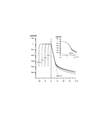
Figure 1: Calculated charging-discharging curves for different $\theta$ ($\beta=1$).

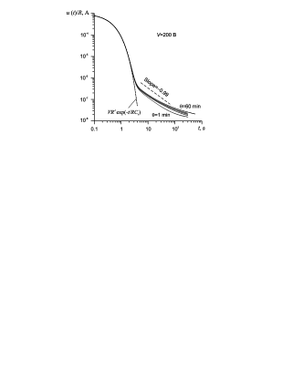
Figure 2: Experimental discharging curves for paper capacitor.

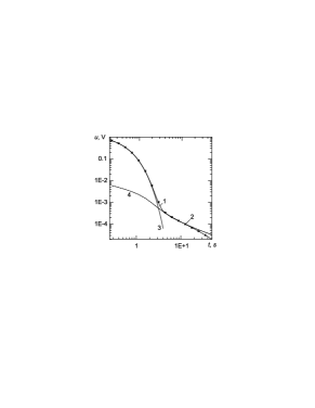
Figure 3: Comparison of numerical results (2) with experimental results (1) for paper capacitor $\theta=300$  , $\tau\approx 0,4$ c^-1. Parameter $\alpha$ is equal to 0,998. 3 – exponential function; 4 – difference between theoretical curve and exponential function.

Figure 4: Experimental discharging curve for electrolyte capacitor ($\theta=3600$  ).

5 Comparison of numerical results with experimental data

We compute charging-discharging curves with the help of constructed algorithm for $\alpha=0.998$. Charging durations are $\theta=10$, 7.5, 5, 2.5 seconds. The voltage falls according to the Debye exponential law for a long time but after some crossover moment we observe splitting with respect to different values of $\theta$ and transition to non-Debye power laws. It seems as if the memory returns to the system after some interval of time. Such behavior was called in (Uchaikin & Uchaikin (2005)) the regeneration memory effect. When $\alpha=1$ the relaxation follows the Debye law and does not depend on $\theta$: the memory is absent.

Experimental measurements (see, Uchaikin et al. (2008a)) were carried out in the following way. At the first time capacitor was shunted through the resistor $R$ and ammeter. Necessary bias voltage was applied by a power source. The capacitor was being charged during time $\theta$. After charging time $\theta$ capacitor became shunted again. The capacitor consists of technical paper impregnated by oil. Its stationary capacitance equals $2\cdot 10^{-6}$ F. For current limitation the resistor $2\cdot 10^{5}$ Ohm was chosen. Voltage of power source is 200 V.

Thus, experimental data presented in Uchaikin et al. (2008a) and given in Fig. 3 confirm the behavior predicted by calculation. Relaxation does not depend on the charging prehistory in some time domain but after enough large time process becomes dependent on charging history.

In Fig. 4 the comparison of calculated discharging process (points) and experimental data (solid line) is given. It was used just one parameter adjusted, $\alpha$ ($\beta=1$). Theoretical and experimental solutions are in a good agreement. Some deviation occurs at large times.

For charging-discharging process the transition from one power decaying law ($t^{-\alpha}$) to another ($t^{-\alpha-1}$) is theoretically predicted in the case of quite large charging times $\theta$. This transition is quite difficult for observation in experiment, because it occurs at large times. Nevertheless this change of exponents in power decaying law has been experimentally observed for electrolyte capacitor. Charging time was equal to an hour.

6 Conclusion

Let us summarize what we represent in this article. Fractional relaxation equation (5) and fractional wave equation (9) for dielectrics with the response function of the Havriliak-Negami type are considered. The explicit expression for the fractional operator in these equations is obtained. The Monte Carlo algorithm for calculation of action of this operator and of the inverse one is constructed. The algorithm is derived from the Bochner-Phillips relation for a semigroup generated by a fractional power of initial infinitesimal operator. The method is based on averaging procedure over ensembles of one-sided stable variables.

Relaxation functions calculated numerically according to this scheme coincide with analytical functions obtained earlier by other authors. The algorithm represents a numerical way of calculation in relaxation problems with arbitrary initial and boundary conditions.

The case, when $\alpha$ is close (but not equal) to 1 and $\beta=1$, is considered in more details. Numerical calculations show that in this case does almost not depend on the prehistory and approximately coincides with up to some value of argument, after which the situation changes. Namely, the solutions with different prehistories reveal different behavior of the inverse power type on the contrary to the exponential behavior in the case. Such phenomena named memory regeneration phenomena in previous publications of the authors are confirmed by experiments with dielectric capacitors.

Authors are grateful to Dr. S. Ambrozevich for kindly presented experimental results and to Prof. V. Uchaikin for fruitful discussions.

References

- Aydiner (2005) Aydiner Ekrem (2005). Anomalous rotational relaxation: A fractional Fokker-Planck equation approach. Phys. Rev. E 71, 046103.
- Bouchaud & Georges (1990) Bouchaud, J. P., Georges, A. (1990). Anomalous diffusion in disordered media: statistical mechanisms, models and physical applications. Physics Reports, 195, 127–293.
- Coffey et al. (2002) Coffey, W. T., Kalmykov, Yu. P., Titov, S. V. (2002). Anomalous dielectric relaxation in the context of the Debye model of noninertial rotational diffusion. J. Chem. Phys. 116, 6422.
- Cole & Cole (1941) Cole, K. S., Cole, R. H. (1941). Dispersion and absorption in dielectrics. Journal of Chemical Physics, 9, 341.
- Davidson & Cole (1951) Davidson, D. W., Cole, R. H. (1951). Dielectric relaxation in glycerol, propylene glycol, and n-propanol. Journal of Chemical Physics, 19, 1484.
- Debye (1954) Debye, P. (1954). Polar Molecules. Dover, New York.
- Déjardin (2003) Déjardin, J.-L. Fractional dynamics and nonlinear harmonic responses in dielectric relaxation of disordered liquids. Phys. Rev. E 68, 031108.
- Fröhlich (1958) Fröhlich, H. (1958). Theory of Dielectrics. 2nd ed. Oxford University Press, Oxford.
- Glöckle (1993) Glöckle, W. G., Nonnenmacher, T. F. (1993). Fox function representation of non-Debye relaxation processes. Journal of Statistical Physics, 71, 741.
- Havriliak & Negami (1966) Havriliak, S., Negami S. (1966). A complex plane analysis of -dispersions in some polymer systems. Journal of Polymer Science, 14, 99.
- Hilfer (2000) Hilfer, R. (2000). Applications of Fractional Calculus in Phisics. World Scientific.
- Jonscher (1977) Jonscher, A. K. (1977). The “universal” dielectric response. Nature, 267, 673.
- Jonscher (1996) Jonscher, A. K. (1996). Universal Relaxation Law. Chelsea-Dielectrics Press, London.
- Jurlewicz & Weron (2000) Jurlewicz, A., Weron, K. (2000). Relaxation dynamics of the fastest channel in multichannel parallel relaxation mechanism. Chaos, Solitons and Fractals, 11, 303.
- Metzler & Klafter (2000) Metzler, R., Klafter, J. (2000). The random walk’s guide to anomalous diffusion: a fractional dynamics approach. Physics Reports, 339, 1–77.
- Nigmatullin (1984) Nigmatullin R. R. (1984). To the theoretical explanation of the “universal response”. Phys. Stat. Sol.(b), 123, 739-745.
- Nigmatullin & Ryabov (1997) Nigmatullin, R. R., Ryabov, Ya. E. Cole-Davidson dielectric relaxation as a self-similar relaxation process. Physics of Solid State, 39, 87.
- Nigmatullin et al. (2003) Nigmatullin, R. R., Osokin, S. I., Smith, G. (2003). The justified data-curve fitting approach: recognition of the new type of kinetic eqations in fractional derivatives from analysis of raw dielectric data. J. of Physics D: Applied Physics, 36, 2281-2294.
- Nigmatullin (2005) Nigmatullin, R. R. (2005). Theory of dielectric relaxation in non-cristalline solids: from a set of micromotions to the averaged collective motion in the mesoscale region. Physica B, 358, 201-215.
- Novikov et al. (2005) Novikov, V. V., Wojciechowski, K. W., Komkova, O. A., Thiel, T. (2005). Anomalous relaxation in dielectrics. Equations with fractional derivatives. Material Science – Poland, 23, 977.
- Podlubny (1999) Podlubny, I. (1999). Fractional Differential Equations. Academic Press.
- Ramakrishnan & Lakshmi (1987) Ramakrishnan, T. V., Raj Lakshmi, M. (1987). Non-Debye Relaxation in Condensed Matter. World Scientific, Singapore.
- Samko et al. (1993) Samko, S. G., Kilbas, A. A., Marichev, O. I. (1993). Fractional Integrals and Derivatives – Theory and Application. Gordon and Breach, New York.
- Sibatov & Uchaikin (2009) Sibatov, R. T., Uchaikin, V. V. (2009). Fractional differential approach to dispersive transport in semiconductors. Physics Uspekhi, 52, 1019–1043.
- Tarasov (2008a) Tarasov, V. E. (2008). Fractional equations of Curie-von Schweidler and Gauss laws. J. Phys.: Condens. Matter, 20, 145212.
- Tarasov (2008b) Tarasov, V. E. (2008). Universal Electromagnetic Waves in Dielectric. Journal of Physics: Condensed Matter, 20, 175223.
- Uchaikin (2003) Uchaikin V. V. (2003). Relaxation processes and fractional differential equations. International Journal of Theoretical Physics, 42, 121-134 (2003).
- Uchaikin & Uchaikin (2005) Uchaikin, V. V., Uchaikin, D. V. (2005). About memory regeneration effect in dielectrics. Scientist Notes of Ulyanovsk State University. Physical Series, 1(17), 14 (in Russian).
- Uchaikin & Uchaikin (2007) Uchaikin, V. V., Uchaikin, D. V. (2007). Proc. Int. Conf. on Chaos, Complexity and Transport (France, Marseille) p. 337.
- Uchaikin (2008) Uchaikin, V. V. (2008). Method of Fractional Derivatives. Artishok, Ulyanovsk (in Russian).
- Uchaikin et al. (2008a) Uchaikin, V. V., Ambrozevich, S. A., Sibatov, R. (2008a) T. About memory phenomenon in dielectrics. Proc. XI Int. Conf. on “Physics of Dielectrics” (Saint-Petersburg) p. 129.
- Uchaikin et al. (2008b) Uchaikin, V. V., Cahoy, D. O., Sibatov, R. T. (2008b). Fractional processes: from Poisson to branching one. International Journal of Bifurcation and Chaos, 18, 2717–2725.
- Uchaikin & Sibatov (2009) Uchaikin, V. V., Sibatov, R. T. (2009). Statistical model of fluorescence blinking. Journal of Experimental and Theoretical Physics, 109, 537- 546.
- Uchaikin et al. (2009) Uchaikin, V. V., Sibatov, R. T., Uchaikin, D. V. Memory regeneration phenomenon in dielectrics: the fractional derivative approach. Physica Scripta 136 (2009) 014002.
- Weron (1991) Weron, K. (1991). How to obtain the universal response law in the Jonscher screened hopping model for dielectric relaxation. Phys.: Condens. Matter 3, 221.
- Weron & Kotulski (1996) Weron, K., Kotulski, M. (1996). On the equivalence of the parallel channel and the correlated cluster relaxation models. Journal of Statistical Physics, 88, 1241.
- West et al. (2002) West, B. J., Bologna, M., Grigolini, P. (2002). Physics of Fractal Operators. Springer-Verlag, New York.