Truncated Lévy statistics for
transport in disordered semiconductors

Abstract

Probabilistic interpretation of transition from the dispersive transport regime to the quasi-Gaussian one in disordered semiconductors is given in terms of truncated Lévy distributions. Corresponding transport equations with fractional order derivatives are derived. We discuss physical causes leading to truncated waiting time distributions in the process and describe influence of truncation on carrier packet form, transient current curves and frequency dependence of conductivity. Theoretical results are in a good agreement with experimental facts.

,

1 Introduction

Various transport regimes can be observed in disordered semiconductors: normal regime characterized by Gaussian statistics and standard diffusion equation, and different types of anomalous (non-Gaussian) transport. Among anomalous transport regimes, the dispersive transport is distinguished especially (Scher & Montroll (1975); Zvyagin (1984); Madan & Shaw (1988)). The dispersive diffusion packet has a non-Gaussian form, but even so it maintains its shape and its spatial extent depends on time. In other words, the process reveals the property of self-similarity (Scher & Montroll (1975)). Dispersive transient current curves are sufficiently differ from the normal ones corresponding to Gaussian transport. Current decays according to very stretched law, two power law sections are picked out: $I(t)\propto t^{-1+\alpha}$ for $t<t_{\rm T}$, and $I(t)\propto t^{-1-\alpha}$ for $t>t_{\rm T}$. The parameter $0<\alpha<1$ called the dispersion parameter depends on material structure and transport mechanism. For some mechanisms, temperature dependence is observed (Zvyagin (1984)). Scher & Montroll (1975) have broken through in understanding of probability causes of dispersive transport, $\alpha$ is interpreted as an exponent of power law asymptotes in a distribution of sojourn times $T$ in localized states (waiting times). Since $\alpha<1$, the mean value $\langle\tau\rangle$ diverges. This leads to non-decreasing relative fluctuations of the number of jumps between localized states. As a consequence we have non-Gaussian form of a diffusion packet and anomalous law of packet widening ($\Delta\propto t^{\alpha/2}$).

The known approaches (such as the Scher-Montroll model (1975), the Arkhipov-Rudenko theory (1982, 1983)) connect the anomalous-normal transition in the same material with increase of $\alpha$ to 1 because of changing outer conditions (for example, temperature). Here, we consider another case, the transition occurs due to changes of scale parameters. For small transient times, i. e. small values of sample thickness and/or large values of voltages, normalized transient current curves are practically universal and these curves correspond to dispersive transport. But in samples with larger thickness, or at smaller voltages (at the same temperatures), transient current curves have plateau (Bässler (1993); Tyutnev et al. (2005)), that is typical for Gaussian transport. Results in this case are often described in frames of the quasi-equilibrium transport theory. In other words, at increasing transient times, the tendency towards the quasi-Gaussian statistics is observed. This tendency can not be explained by change of the dispersive parameter $\alpha$, it is a spatiotemporal scale effect.

Electron transport in polymers is usually modelled as a hopping process. Experimental time-of-flight results for polymers come to an agreement with the theory, when the Gaussian form of an energy distribution of localized states is taken (Bässler (1993)). Transition from dispersive type of transport to the quasi-Gaussian one can be explained by such form of density of localized states.

The goal of the present paper is to give a probabilistic interpretation of transition from the dispersive transport regime to the quasi-Gaussian one due to change of the scale parameters characterizing the process. The additional question is to determine main features of energetic and/or spatial distributions of traps leading to the discussed phenomenon. Truncated Lévy distributions introduced by Mantegna & Stanley (1994) play an important role in our interpretation. We derive correspondent equations with fractional order derivatives and discuss the influence of truncation on transient current curves and frequency dependence of conductivity.

2 Dispersive transport and fractional differential approach

Dispersive (non-Gaussian) transport (Madan & Shaw (1988), Zvyagin (1984)) is observed in many disordered materials differ in its microscopical structure. A comparison of available data suggests the presence of universal transport properties unrelated to the detailed atomic and molecular structure of a substance. The fractional differential approach is often applied to description of dispersive transport (Barkai (2001); Uchaikin & Sibatov (2005, 2008); Sibatov & Uchaikin (2009)).

The Riemann-Liouville type fractional derivatives

$${}_{0}\textsf{D}_{t}^{\alpha}f(t)=\frac{1}{\Gamma(1-\alpha)}\frac{d}{dt}\int\limits_{0}^{t}\frac{f(t^{\prime})dt^{\prime}}{(t-t^{\prime})^{\alpha}},\quad 0<\alpha<1$$

were for the first time applied to description of dispersive transport by Arkhipov et al. (1983b). The authors expressed the relationship between concentrations of free and localized carriers through the fractional integral. In later papers they use a different approximate relation between concentrations of localized and free carriers, which they called the master dispersive transport equation. This relation is believed to hold for any density of localized states and permits expressing results through elementary functions in the case of an exponential density. The Arkhipov-Rudenko master equation leads to a diffusion equation with a variable diffusion coefficient and mobility (Arkhipiov et al. (1983a)).

On the base of the kinetic trapping-emission equations, Tiedje (1984) derived a transport equation for free carrier concentration. The inverse Laplace transform of this equation is nothing but a fractional differential equation (Sibatov & Uchaikin (2007)).

Barkai (2001) made use of the fractional Fokker-Planck equation to account for transient photocurrent relaxation in amorphous semiconductors. He showed the agreement between selected results of the fractional differential approach and results predicted by the Scher-Montroll model (1975).

Power-law decay of photoluminescence in amorphous semiconductors was described in Refs (Seki et al. (2003, 2006)) in frame of the generalized random walk model with recombination by tunnel radiative transitions. Recombination was limited by dispersive diffusion of the carriers. In the framework of this model, Seki et al. (2006) compiled a fractional differential equation for the first passage time distribution density. The recombination rate was found using the integral Laplace transform of this equation.

As shown in Refs (Uchaikin (1999); Sibatov & Uchaikin (2007)), the main asymptotic terms in the Scher-Montroll model satisfy fractional differential equations, the Green functions of which are fractionally stable densities.

3 The Scher-Montroll model

Continuous time random walk (CTRW) model, introduced by Scher & Montroll (1975), provided the first detailed explanation of all the main patterns of current behavior in time-of-flight experiments with amorphous semiconductors.

The main assumptions of this model are as follows:

1. The transport of charge carriers is a jumplike random walk in which the walkers change their positions at random instants of time.

2. Carrier jumps are independent of one another, and time intervals between them (waiting times) are independent, identically distributed random variables $T$.

3. Waiting times are characterized by asymptotically power-law distribution:

   $$\textsf{P}\{T>t\}\propto t^{-\alpha},\quad t\rightarrow\infty,\qquad 0<\alpha<1.$$ (1)

Scher & Montroll (1975) simulated charge transfer in disordered semiconductors as carrier hopping within the model grid of localized states. The grid constitutes a regular cubic lattice, each cell of which contains randomly distributed sites (localized states). The waiting time till the next hopping depends on the distance to the nearest neighbor sites. The cell residence time distribution can obey the power law owing to site spatial disorder in a cell.

As is known, the description of normal transport is based on the central limit theorem of the probability theory. For random quantities distributed according to asymptotically power law, divergence of dispersion for ${\alpha<2}$ and divergence of mathematical expectation for $\alpha<1$ make this theorem inapplicable, which necessitates the application of the generalized limit theorem.

The generalized limit theorem. Let random quantities $X_{j}$ be independent and identically distributed, and satisfy the following conditions

$${\sf P}(X>x)\sim a_{+}x^{-\alpha},\qquad x\to\infty,$$

$${\sf P}(X<-x)\sim a_{-}x^{-\alpha},\qquad x\to\infty,$$

$0<\alpha\leq 2,\ a_{+}\geq 0,a_{-}\geq 0$ and $a_{+}+a_{-}>0$. Then, $A_{n}$ and $B_{n}>0$, sequences exist such that, as $n\to\infty$, one finds

$$\left.\left(\sum_{j=1}^{n}X_{j}-A_{n}\right)\right/B_{n}\mathop{\sim}\limits^{d}S^{(\alpha,\beta)},$$

where $S^{(\alpha,\beta)}$ is the stable random variable with exponent $\alpha$ and asymmetry parameter ${\beta=(a_{+}-a_{-})/(a_{+}+a_{-})}$. Stable random quantities can be defined through characteristic functions having the form (form A) (Uchaikin & Zolotarev (1999)):

$$g^{(\alpha,\beta)}(k)=\exp\{-|k|^{\alpha}[1-i\beta\tan(\alpha\pi/2)\ \mathrm{sign}(k)]\},\qquad\alpha\neq 1,$$

$$g^{(1,\beta)}(k)=\exp(-|k|).$$

Certainly, there are an infinite number of sequences of normalizing coefficients $A_{n},B_{n}$ showing similar asymptotic behavior as $n\to\infty$. By way of example, they can be defined in the following way ($a=\langle X\rangle$ and $c=a_{+}+a_{-}$):  
$\alpha=2$ $A_{n}=na,$ $B_{n}=\sqrt{cn\ln n}$, $\alpha\in(1,2)$ $A_{n}=na,$ $B_{n}=\left(\pi cn/[2\Gamma(\alpha)\sin(\alpha\pi/2)]\right)^{1/\alpha}$, $\alpha=1$ $A_{n}=\beta cn\ln n,$ $B_{n}=\pi cn/2$, $\alpha\in(0,1)$ $A_{n}=0,$ $B_{n}=\left(\pi cn/[2\Gamma(\alpha)\sin(\alpha\pi/2)]\right)^{1/\alpha}$.

In the Scher-Montroll model, waiting times $T$ (positive random quantities) are distributed according to an asymptotically power law. Therefore, at macroscopic scales, the first passage time distribution, conduction current density, and concentration of delocalized carriers considered as functions of time should have the form of stable density distribution.

The main characteristics of the CTRW model are waiting time and jump vector distributions, $\psi(t)$ and $p(\mathbf{r})$, respectively. Spatial distribution density $p(\mathbf{r},t)$ of a particle executing random walks and initially located at the origin of coordinates is defined in terms of the Fourier-Laplace transform (Montroll & Weiss (1965))

$$\widehat{\widetilde{p}}(\mathbf{k},s)=\frac{1-\widetilde{\psi}(s)}{s}\frac{1}{1-\widehat{p}(\mathbf{k})\widetilde{\psi}(s)},$$ (2)

where

$$\widehat{\widetilde{p}}(\mathbf{k},s)=\int\limits_{\mathbf{R}}d\mathbf{r}\ e^{i\mathbf{k}\mathbf{r}}\int\limits_{0}^{\infty}dt\ e^{-st}p(\mathbf{r},t)$$

is the Fourier-Laplace transform of normalized particle concentration, $\widetilde{p}(\mathbf{k})$ is the Fourier transform of path distribution density, and $\widehat{\psi}(s)$ is the Laplace transform of waiting time distribution density. Substituting into Eq. (2) the asymptotic series expansion of the Laplace image of waiting time distribution density with the power-law tail

$$\widehat{\psi}(s)\sim 1-s^{\alpha}/c^{\alpha},\quad s\ll c,$$

along with asymptotic expansion of the Fourier image of path distribution density:

$$\widetilde{p}(\mathbf{k})\sim 1+\mathbf{c}_{1}i\mathbf{k}-c_{2}k^{2},\quad\ |\mathbf{k}|\ll 1/|\mathbf{c}_{1}|,$$

and applying the Tauberian theorem, we obtain

$$\widehat{\widetilde{p}}(\mathbf{k},s)=\frac{c^{-\alpha}s^{\alpha-1}}{-\mathbf{c}_{1}i\mathbf{k}+c_{2}k^{2}+s^{\alpha}/c^{\alpha}}.$$

Rewriting the last expression in the form

$$[s^{\alpha}-\mathbf{c}_{1}c^{\alpha}i\mathbf{k}+c_{2}c^{\alpha}k^{2}]\ \widehat{\widetilde{p}}(\mathbf{k},s)=s^{\alpha-1}$$

and applying inverse Fourier and Laplace transformations yield

$$_{0}\textsf{D}^{\alpha}_{t}p(\mathbf{r},t)+\mathbf{K}\nabla p(\mathbf{r},t)-C\nabla^{2}p(\mathbf{r},t)=\frac{t^{-\alpha}}{\Gamma(1-\alpha)}\delta(\mathbf{r}),$$ (3)

where $\mathbf{K}$ and $C$ are vectorial and scalar constants.

4 Truncated waiting time distributions

It has been emphasized above that the self-similar dispersive transport in disordered semiconductors is characterized by asymptotically power law distributions of sojourn times $T$ of carriers (electrons and/or holes) in localized states: $\textsf{P}\{T>t\}\propto t^{-\alpha}$, $t\rightarrow\infty$, where $0<\alpha<1$ is the dispersion parameter. Mean value of such random variables diverges.

It is naturally to suppose that an asymptotically power law distribution of waiting times can be truncated. This truncation can be caused by finite values of mobility gap at multiple trapping or by limitation of jump lengths at hopping. Secondary mechanism acting in parallel to the main transport mechanism can be responsible for the truncation. We shall consider an influence of truncation of power law distributions of waiting times on properties of dispersive transport. This influence should become apparent in scale effects.

Mantegna and Stanley (1994) introduced truncated Lévy flights, a process showing a slow convergence to a Gaussian. The truncated Lévy flight is a Markovian jump process, with the length of jumps showing a power-law behavior up to some large scale. At large scales distribution has cutoffs and thus have finite moments of any order. Smoothly (exponentially) truncated Lévy flights, introduced by Koponen (1995), constructed on Mantegna and Stanley’s ideas, allows to give a convenient analytic representation of results.

In our model, jump lengths are distributed exponentially and waiting times have asymptotically truncated power law distributions. We take this distribution in the form

$$\Psi(t)=\textsf{P}\{T>t\}\sim\frac{(ct)^{-\alpha}}{\Gamma(1-\alpha)}\exp(-\gamma t),$$ (4)

$$\quad\gamma\ll c,\qquad t\gg c^{-1}.$$

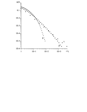
Figure 1: Waiting time PDF’s for different types of densities of localized states in the multiple trapping model: exponential (1), Gaussian (2) and rectangular (3).

Since the ”heavy” power law tail is truncated, all moments of random variable are finite, and consequently, a distribution of a sum of large number of such random variables tends to the Gaussian law. However, this convergence is very slow and stable Lévy distributions play a role of intermediate asymptotics.

In Fig. 1, normalized waiting time distributions numerically calculated for three forms of density of states (exponential, Gaussian and rectangular) in the multiple trapping model are presented. For all three cases, an average energy of states $\varepsilon_{0}$ is the same. For exponential DOS waiting times are distributes according to the asymptotical power law with the exponent $\alpha=\varepsilon_{0}/kT$. For the case of the Gaussian DOS, sojourn times in traps are distributed according to a wide law but all moments finite. For the case of rectanguler DOS, waiting times have distribution that can be approximated by a stretched exponential law.

Transport is dispersive in all time scales only in the case of ideal exponential energy distribution of localized states. For two other DOS, transport takes features of the normal transport in asymptotics of large times.

5 Transport equation for the case of truncated waiting time distributions

Connection between concentrations of delocalized (conduction) $n_{\mathrm{c}}$ and trapped $n_{\mathrm{t}}$ carriers is expressed by the formula

$$n_{\mathrm{t}}(\mathbf{r},t)=\int\limits_{0}^{t}\tau_{0}^{-1}n_{\mathrm{c}}(\mathbf{r},t^{\prime})\ \Psi(t-t^{\prime})\ dt^{\prime},$$

where $\tau_{0}$ is a mean time of delocalized state. Passing on to Laplace transforms, taking into account the relation

$$\hat{\Psi}(s)=\int\limits_{0}^{\infty}e^{-st}\Psi(t)\ dt\sim c^{-\alpha}(s+\gamma)^{\alpha-1},\quad s\ll c,$$

we obtain $\hat{n}_{\mathrm{t}}(\mathbf{r},s)\sim c^{-\alpha}\tau_{0}^{-1}(s+\gamma)^{\alpha-1}\hat{n}_{\mathrm{c}}(\mathbf{r},s)$. The inverse Laplace transformation leads to the equation with derivative of fractional order:

$$n_{\mathrm{c}}(\mathbf{r},t)\sim c^{\alpha}\tau_{0}\ e^{-\gamma t}{{}_{0}\textsf{D}_{t}^{1-\alpha}}e^{\gamma t}\ n_{\mathrm{t}}(\mathbf{r},t),\qquad t\gg c^{-1}.$$ (5)

Substituting the last relation into the continuity equation

$$\frac{\partial n(\mathbf{r},t)}{\partial t}+\mathrm{div}\left(\mu\mathbf{E}\ n_{\mathrm{c}}(\mathbf{r},t)-D\ \nabla n_{\mathrm{c}}(\mathbf{r},t)\frac{}{}\right)=0$$

and taking into account the fact that most of carriers are trapped, i. e. $n(\mathbf{r},t)\approx n_{\mathrm{t}}(\mathbf{r},t)$, we arrive at

$$\frac{\partial n(\mathbf{r},t)}{\partial t}+$$

$$+\mathrm{div}\left[e^{-\gamma t}{{}_{0}\textsf{D}_{t}^{1-\alpha}}e^{\gamma t}\ \left(\mathbf{K}\ n(\mathbf{r},t)-C\ \nabla n(\mathbf{r},t)\right)\right]=0,$$ (6)

where $\textbf{K}=c^{\alpha}\tau_{0}\mu\textbf{E}$, $C=c^{\alpha}\tau_{0}D$ are coefficients, and $\mu,\ D,\ \mathbf{E}$ are a mobility, a diffusion coefficient and a field intensity, respectively. If $\alpha\rightarrow 1$, Eq. (6) becomes the standard Fokker-Planck equation describing the normal transport. When $\gamma=0$, the equation coincides with the dispersive transport equation.

6 Scale effect of transition from the dispersive regime to the Gaussian one

Fig. 2 represents numerically calculated spatial distributions for one-sided random walks. With different waiting time distributions, one can see the transition from fractionally stable statistics to Gaussian statistics for waiting time distribution having truncated power law tail. The upper graph represents results for exponentially distributed times between jumps. In the middle graph, waiting times are not truncated, the exponent of the power law tail is equal to 0.5. In the lower graph, waiting time distribution has the sharp truncation at time $\tau_{\mathrm{tr}}=1500$ (arbitrary units). The exponential distribution of waiting times has the same mathematical expectation as truncated power law in the lower graph. In the case of exponentially distributed waiting times, we see the fast convergence to the Gaussian distribution, in the second case, the distribution becomes fractionally stable law at some time $t$ and maintains the form for all following times. In case of truncated power law tails, the crossover between fractionally stable and Gaussian statistics is observed.

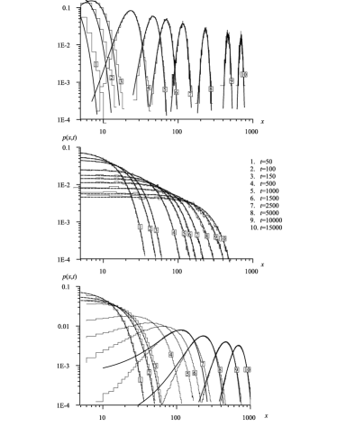
Figure 2: The transition from the fractionally stable statistics to the Gaussian one in the case of a one-sided random walk with waiting times distributed according to law having truncated power law tail. Solid lines represent Gaussian PDFs, dotted lines correspond to fractionally stable densities.

Conduction current density at pulsed injection for the case of exponentially truncated power-law waiting time distributions is expressed as

$$j(x,t)=eN\exp\left[\frac{x}{l}{\left(\frac{\gamma}{c}\right)}^{\alpha}-\gamma t\right]\times\ \ \ \qquad\ \qquad\ \qquad$$

$$\ \qquad\ \qquad\times c\left(\frac{x}{l}\right)^{-1/\alpha}g^{(\alpha)}\left(ct\left(\frac{x}{l}\right)^{-1/\alpha}\right).$$ (7)

Transient current density is found by substituting this expression into the formula

$$I(t)=\frac{1}{L}\int\limits_{0}^{L}j(x,t)dx.$$

If $\alpha=1/2$, the expression for transient current takes the form:

$$I(t)=\frac{eNl\sqrt{c}}{L}\left\{\frac{\exp(-\gamma t)-\exp\left(-\left(\sqrt{\gamma t}-\frac{1}{2\sqrt{\tau}}\right)^{2}\right)}{\sqrt{\pi t}}+\right.$$

$$\left.+\sqrt{\gamma}\left[\mathrm{erf}(\sqrt{\gamma t})-\mathrm{erf}\left(\sqrt{\gamma t}-\frac{1}{2\sqrt{\tau}}\right)\right]\right\}$$ (8)

Fig. 3 illustrates transformation of transient current curves with increasing $L/l$-ratio. When the time of flight is much smaller than the truncation time $\gamma^{-1}$, the transport remains dispersive and does not pass to Gaussian asymptotics. If $t_{\mathrm{tr}}$ is compared with $\gamma^{-1}$ the shape of the transient current curves undergoes modification, and they become inconsistent with the curves for normal and dispersive transport. For $t_{\mathrm{tr}}\gg\gamma^{-1}$, transport in the long-time asymptotic regime becomes quasi-Gaussian.

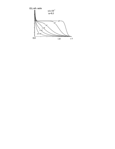
Figure 3: Transient photocurrent in the case of truncated power law distribution of waiting times for different values of $L/l$-ratio.

7 Frequency dependence of conductivity

The frequency dependence of the real component of conductivity in disordered semiconductors is usually fairly well described by the power law:

$$\mathrm{Re}\ \sigma(\omega)=A\omega^{\gamma},$$ (9)

where the exponent $\gamma$ normally takes on values from 0.7 to 1 (Zvyagin (1984)). The dependence of such type is characteristic of a very broad class of materials.

Conductivity is related to mobility by the expression

$$\sigma(\omega)=e\eta\mu(\omega).$$

Here, $\eta$ is the concentration of effective carriers. The Nyquist formula (generalized Einstein relation) linking mobility with the diffusion coefficient at nonzero frequencies has the form

$$\mu(\omega)=(e/kT)D(\omega),$$

where the noise spectrum according the Wiener-Khintchin theorem is expressed through the Fourier transform of the velocity autocorrelation function

$$\mathrm{Re}\ D(\omega)=\int\limits_{0}^{\infty}\cos(\omega t)\langle v(t)v(0)\rangle dt.$$ (10)

This formula is important in that ”a knowledge of the fluctuations of the equilibrium ensemble in the absence of the electric field permits a calculation of the linear response of the system (mobility)” (Scher & Lax (1973a)). Scher & Lax showed that relation (10) can be written out as:

$$D(\omega)=-\frac{1}{6}\ \omega^{2}\int\limits_{0}^{\infty}dt\ e^{-i\omega t}\left\langle[\mathbf{r}(t)-\mathbf{r}(0)]^{2}\right\rangle.$$ (11)

The latter relation is possible to rewrite in the form

$$D(\omega)=-\omega^{2}\int\limits_{0}^{\infty}dx\ x^{2}\left[\widetilde{n}(x,s)\right]_{s=i\omega},$$ (12)

where $\widetilde{n}(x,s)$ is the Laplace image of $n(x,t)$ with respect to $t$.

Equation (6) for one-dimensional case without field assumes the form:

$$\frac{\partial n(x,t)}{\partial t}=C\ e^{-\gamma t}\frac{\partial^{1-\alpha}}{\partial t^{1-\alpha}}e^{\gamma t}\ \frac{\partial^{2}n(x,t)}{\partial x^{2}}.$$

The Laplace transform of this equation yields

$$s\ \widetilde{n}(x,s)=C\ (s+\gamma)^{1-\alpha}\ \frac{\partial^{2}\widetilde{n}(x,s)}{\partial x^{2}}+\delta(x).$$

Substituting the solution of this equation,

$$\widetilde{n}(x,s)=\frac{s^{-1/2}(s+\gamma)^{(\alpha-1)/2}}{\sqrt{C}}\exp\left(-\frac{|x|}{\sqrt{C}}\ \sqrt{s(s+\gamma)^{\alpha-1}}\right)$$

into relation (12) gives

$$D(\omega)=2C(\gamma+i\omega)^{1-\alpha}.$$

Hence follows

$$\mathrm{Re}\ \sigma(\omega)=(e^{2}\eta/kT)\ \mathrm{Re}\ D(\omega)=$$

$$=2C(e^{2}\eta/kT)\ (\gamma^{2}+\omega^{2})^{(1-\alpha)/2}\cos((1-\alpha)\arctan(\omega/\gamma)).$$ (13)

For frequencies $\omega\gg\gamma$, it is easily shown that

$$\mathrm{Re}\ \sigma(\omega)=2C(e^{2}\eta/kT)\ \omega^{1-\alpha}\sin(\pi\alpha/2).$$

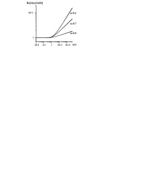
Figure 4: Theoretical frequency dependencies of conductivity for different $\alpha$ values.

Figure 4 represents frequency-dependent conductivity curves calculated from Eq. (13). Formula (13) predicts the power-law dependence of conductivity on $\omega$ at high frequencies in the dispersive transport case. The exponent may acquire values from 0 to 1; in normal transport ($\alpha\rightarrow 1$), conductivity is totally frequency independent. In transport driven by the multiple trapping mechanism, exponent $\alpha$ grows linearly with temperature. Consequently, the exponent ${s=1-\alpha}$ in the frequency dependence of conductivity in the case of alternating current must linearly decrease with increasing temperature. Such temperature behavior has been reported for a variety of semiconductors (see, for instance, Ghosh et al. (2006)).

8 Conclusion

Here, transition from the dispersive transport regime to the quasi-Gaussian one in disordered semiconductors is interpreted in terms of truncated Lévy distributions of waiting times. So, polymer with Gaussian density of localized states is not exclusive representative of materials that can show such behavior. The phenomenon is more general and it is based on statistical rules such as generalized limit theorem. Analytical results are supported by numerical simulations.

References

- Arkhipiov et al. (1983a) V. I. Arkhipov, A. I. Rudenko, A. M. Andriesh et al. Non-stationary injection currents in disordered solids. Kishinev, 1983.
- Arkhipov et al. (1983b) V. I. Arkhipov, Yu. A. Popova, A. I. Rudenko. Semiconductors 17:1159, 1983.
- Aroutiounian et al. (2000) V. M. Aroutiounian, M. Zh. Ghoolinian and H. Tributsch. Fractal model of porous semiconductor. Applied Surface Science 162:122–132, 2000.
- Barkai (2001) E. Barkai. Fractional Fokker-Planck equation, solution, and application. Phys. Rev. E 63:046118, 2001.
- Bässler (1993) H. Bässler. Charge transport in disordered organic photoconductors. Phys. Stat. Sol. (b) 175:15–56, 1993.
- Ghosh et al. (2006) P. Ghosh, A. Sarkar, A. K. Meikap, S. K. Chattopadhyay, S. K. Chatterjee, M. Ghosh. Electron transport properties of cobalt doped polyaniline. J. Phys. D: Appl. Phys. 39:3047–3052, 2006.
- Koponen (1995) I. Koponen. Analytic approach to the problem of convergence of truncated L’evy flights towards the Gaussian stochastic process. Phys. Rev. E 52:1197-1199, 1995.
- Madan & Shaw (1988) A. Madan, M. P. Shaw. The Physics and Applications of Amorphous Semiconductors. Academic Press Inc., Boston, 1988.
- Mantegna & Stanley (1994) R. N. Mantegna and H. E. Stanley. Stochastic process with ultraslow convergence to a Gaussian: The truncated Lévy flight Phys. Rev. Letters 73:2946–2949, 1994.
- Montroll & Weiss (1965) E. W. Montroll, G. H. Weiss. Random walks on lattices. J. Math. Phys. 6:167–181, 1965.
- Scher & Lax (1973a) H. Scher and M. Lax. Stochastic transport in a disordered solid. I. Theory. Phys. Rev. B 7:4491–4502, 1973.
- Scher & Lax (1973b) H. Scher and M. Lax. Stochastic transport in a disordered solid. II. Impurity conduction. Phys. Rev. B 7:4502–4519, 1973.
- Scher & Montroll (1975) H. Scher and E. W. Montroll. Anomalous transit-time dispersion in amorphous solids. Phys. Rev. B 12 (1975) 2455-2477.
- Seki et al. (2003) K. Seki, M. Wojcik, M. Tachiya. Recombination kinetics in subdiffusive media. J. Chem. Phys. 119:7525–7533, 2003.
- Seki et al. (2006) K. Seki, M. Wojcik, M. Tachiya. Dispersive-diffusion-controlled distance-dependent recombination in amorphous semiconductors. J. Chem. Phys. 124:044702, 2006.
- Sibatov & Uchaikin (2007) R. T. Sibatov, V. V. Uchaikin. Fractional differential kinetics of charge transport in unordered semiconductors. Semiconductors 41:335 -340, 2007.
- Sibatov & Uchaikin (2009) R. T. Sibatov, V. V. Uchaikin. Fractional differential approach to dispersive transport in semiconductors. Physics Uspekhi 52:1019 -1043, 2009.
- Tiedje (1984) T. Tiedje. Investigations of charge transport in hydrogenated amorphous silicon. In: J. D. Joannoulos and G. Lucovsky (Eds.), The Physics of Hydrogenated Amorphous Silicon II. Electronic and Vibrational Properties. Springer-Verlag, New York, 1984.
- Tyutnev et al. (2005) A. P. Tyutnev, V. S. Saenko, E. D. Pozhidaev, N. S. Kostyukov. Dielektricheskie Svoistva Polimerov v Polyakh Ioniziruyushchikh Izluchenii (Dielektriki i Radiatsiya, Kn. 5) [Dielectric Properties of Polymers in Ionizing Radiation Fields (Dielectrics and Radiation, Book 5)], Moscow: Nauka, 2005.
- Uchaikin & Zolotarev (1999) V. V. Uchaikin and V. M. Zolotarev. Chance and Stability. VSP, Utrecht, tne Netherlands, 1999.
- Uchaikin (1999) V. V. Uchaikin. Subdiffusion and stable laws. J. of Exper. and Theor. Phys. 115:2113–2132, 1999.
- Uchaikin & Sibatov (2005) V. V. Uchaikin and R. T. Sibatov. Fractional derrivatives in theory of semiconductors. Surveys of Appl. and Industr. Math. 12:540–542, 2005.
- Uchaikin & Sibatov (2008) V. V. Uchaikin and R. T. Sibatov. Fractional theory for transport in disordered semiconductors. Communications in Nonlinear Science and Numerical Simulation 13:715 727, 2008.
- Zvyagin (1984) I. P. Zvyagin. Kineticheskie Yavleniya v Neuporyadochennykh Poluprovodnikakh (Kinetic Phenomena in Disordered Semiconductors). Moscow: Izd. MGU, 1984.