Dynamic response of strongly correlated Fermi gases in the quantum virial expansion

Abstract

By developing a quantum virial expansion theory, we quantitatively calculate the dynamic density response function of a trapped strongly interacting Fermi gas at high temperatures near unitarity. A clear transition from atomic to molecular responses is identified in the spectra when crossing from the BCS to BEC regimes, in qualitative agreement with recent Bragg spectroscopy observations. Our virial expansion method provides a promising way to solve the challenging strong-coupling problems and is applicable to other dynamical properties of strongly correlated Fermi gases.

I Introduction

The dynamic structure factor (DSF) plays a fundamental role in understanding quantum many-body systems allanbook : it gives the response of the system to an excitation process that couples to density. Experimental advances in Bragg spectroscopy have now measured the DSF for strongly interacting ultra-cold fermions. At a high momentum transfer, these experiments show evidence for a clear transition from atomic to molecular response when traversing from the BCS to BEC regimesswinexpt . However, while the DSF for weakly interacting bosons is well-studied theoretically and experimentally braggbec , the expected dynamic structure factor of strongly interacting fermions remains unknown, except for a dynamical mean-field approximation combescot ; minguzzi . This is due to the notorious absence of a small parameter for strongly interacting particles. The Bragg experiments create a theoretical challenge: how can one reliably calculate the dynamic structure factor in this strongly interacting regime? Similar challenges also arise when one tries to understand some recent measurements on radiofrequency spectroscopy of strong interacting fermions rfgrimm ; rfketterle ; rfzwierlein .

In this paper, we present a systematic study of the dynamic structure factor of a normal, trapped and strongly interacting Fermi gas at high temperatures. This is achieved by developing a quantum virial expansion for dynamical properties of many-body systems. Our expansion is applicable to arbitrary interaction strengths and has a controllable small parameter. The fugacity $z\equiv\exp(\mu/k_{B}T)\ll 1$ is small since the chemical potential $\mu$ tends to $-\infty$ at large temperatures $T$. We note that dynamical studies using virial expansions have been carried out for classical, untrapped gases Miyazaki . However, previous virial expansion studies of quantum gases were restricted to static properties only jasonho ; ourve . By comparing the virial expansion prediction unitaritycmp with the experimentally measured equation of state nascimbene , we find a wide applicability of the expansion for a trapped Fermi gas: it is valid down to temperatures as low as 0.4$T_{F}$ (see Ref. unitaritycmp for details). Here, $T_{F}$ is the Fermi temperature of a trapped ideal, non-interacting Fermi gas.

Our main results may be summarized as follows. We find a smooth transition in the dynamic structure factor, from an atomic response to a molecular response as the interaction strength increases (Fig. 1). This feature agrees reasonably well with recent experimental measurements although the latter was carried out at lower temperatures. We show that the spin-antiparallel dynamic structure factor provides the most sensitive probe for molecule formation (Figs. 2 and 3). The static structure factor is also obtained as a subset of our results (Fig. 4). These predictions are readily testable experimentally.

II Quantum virial expansion of dynamic structure factor

We start by constructing the virial expansion for the dynamic structure factor $S({\bf q},\omega)$, the Fourier transform of the density-density correlation functions at two different space-time points. Consider a harmonically trapped atomic Fermi gas with an equal number of atoms ($N/2$) in two hyperfine states (referred to as spin-up, $\sigma=\uparrow$, and spin-down, $\sigma=\downarrow$), where $S_{\uparrow\uparrow}({\bf q},\omega)=S_{\downarrow\downarrow}({\bf q},\omega)$ and $S_{\uparrow\downarrow}({\bf q},\omega)=S_{\downarrow\uparrow}({\bf q},\omega)$. To calculate the total dynamic structure factor $S({\bf q},\omega)\equiv 2[S_{\uparrow\uparrow}({\bf q},\omega)+S_{\uparrow\downarrow}({\bf q},\omega)]$, it is convenient to work with the dynamic susceptibility allanbook , $\chi_{\sigma\sigma^{\prime}}\left({\bf r},{\bf r}^{\prime};\tau\right)\equiv-\left\langle T_{\tau}\hat{n}_{\sigma}\left({\bf r},\tau\right)\hat{n}_{\sigma^{\prime}}\left({\bf r}^{\prime},0\right)\right\rangle$, where $\hat{n}_{\sigma}\left({\bf r},\tau\right)$ is the density (fluctuation) operator in spin channel $\sigma$, and $\tau$ is an imaginary time in the interval $0<\tau\leq\beta=1/k_{B}T$.

The DSF is then obtained allanbook from the Fourier components $\chi_{\sigma\sigma^{\prime}}\left({\bf r},{\bf r}^{\prime};i\omega_{n}\right)$ at discrete Matsubara imaginary frequencies $i\omega_{n}=i2n\pi k_{B}T$ ($n=0,\pm 1,...$), via analytic continuation and the fluctuation-dissipation theorem:

$$S_{\sigma\sigma^{\prime}}\left({\bf r},{\bf r}^{\prime};\omega\right)=-\frac{\mathop{\rm Im}\chi_{\sigma\sigma^{\prime}}\left({\bf r},{\bf r}^{\prime};i\omega_{n}\rightarrow\omega+i0^{+}\right)}{\pi(1-e^{-\beta\omega})}\,\,\,.$$

A final Fourier transform with respect to the relative spatial coordinate ${\bf r}-{\bf r}^{\prime}$ leads to $S_{\sigma\sigma^{\prime}}\left({\bf q},\omega\right)$.

Our quantum virial expansion applies to the dynamic susceptibility $\chi_{\sigma\sigma^{\prime}}\left({\bf r},{\bf r}^{\prime};\tau>0\right)$, which is formally expanded as:

$$\chi_{\sigma\sigma^{\prime}}\equiv-\frac{\text{Tr}\left[e^{-\beta\left({\cal H}-\mu{\cal N}\right)}e^{{\cal H}\tau}\hat{n}_{\sigma}\left({\bf r}\right)e^{-{\cal H}\tau}\hat{n}_{\sigma^{\prime}}\left({\bf r}^{\prime}\right)\right]}{\text{Tr}e^{-\beta\left({\cal H}-\mu{\cal N}\right)}}.$$ (1)

At high temperatures, Taylor-expanding in terms of the powers of small fugacity $z\equiv\exp(\mu/k_{B}T)\ll 1$ leads to $\chi_{\sigma\sigma^{\prime}}\left({\bf r},{\bf r}^{\prime};\tau\right)=(zX_{1}+z^{2}X_{2}+\cdots)/(1+zQ_{1}+z^{2}Q_{2}+\cdots)=zX_{1}+z^{2}\left(X_{2}-X_{1}Q_{1}\right)+\cdots$, where we have introduced the cluster functions $X_{n}=-$ Tr${}_{n}[e^{-\beta{\cal H}}e^{\tau{\cal H}}\hat{n}_{\sigma}({\bf r)}e^{-\tau{\cal H}}\hat{n}_{\sigma^{\prime}}({\bf r}^{\prime})]$ and $Q_{n}=$Tr${}_{n}[e^{-\beta{\cal H}}]$, with $n$ denoting the number of particles in the cluster and Tr_n denoting the trace over $n$-particle states of proper symmetry. We shall refer to the above expansion as the virial expansion of dynamic susceptibilities, $\chi_{\sigma\sigma^{\prime}}\left({\bf r},{\bf r}^{\prime};\tau\right)=z\chi_{\sigma\sigma^{\prime},1}\left({\bf r},{\bf r}^{\prime};\tau\right)+z^{2}\chi_{\sigma\sigma^{\prime},2}\left({\bf r},{\bf r}^{\prime};\tau\right)+\cdots,$ where,

$$\chi_{\sigma\sigma^{\prime},1}\left({\bf r},{\bf r}^{\prime};\tau\right) = X_{1},$$

$$\chi_{\sigma\sigma^{\prime},2}\left({\bf r},{\bf r}^{\prime};\tau\right) = X_{2}-X_{1}Q_{1},\ \text{etc}.$$ (2)

Accordingly, we shall write for the dynamic structure factors, $S_{\sigma\sigma^{\prime}}\left({\bf q},\omega\right)=zS_{\sigma\sigma^{\prime},1}\left({\bf q},\omega\right)+z^{2}S_{\sigma\sigma^{\prime},2}\left({\bf q},\omega\right)+\cdots$. It is readily seen that a similar virial expansion holds for other dynamical properties. As anticipated, the determination of the $n$-th expansion coefficient requires the knowledge of all solutions up to $n$-body, including both the eigenvalues and eigenstates. Here we aim to calculate the leading effect of interactions, which contribute to the 2nd-order expansion function. For this purpose, it is convenient to define $\Delta\chi_{\sigma\sigma^{\prime},2}\equiv\left\{\chi_{\sigma\sigma^{\prime},2}\right\}^{(I)}=\left\{X_{2}\right\}^{(I)}$ and $\Delta S_{\sigma\sigma^{\prime},2}\equiv\left\{S_{\sigma\sigma^{\prime},2}\right\}^{(I)}$. The notation $\left\{\right\}^{(I)}$ means the contribution due to interactions inside the bracketed term, so that $\left\{X_{2}\right\}^{(I)}=X_{2}-X_{2}^{(1)}$, where the superscript “1” in $X_{2}^{(1)}$ denotes quantities for a noninteracting system. We note that the inclusion of the 3rd-order expansion function is straightforward, though involving more numerical effort.

To solve the two-fermion problem, we adopt a short-range S-wave pseudopotential for interactions between two fermions with opposite spins, in accord with the experimental situation of broad Feshbach resonances. In an isotropic harmonic trap with potential $V\left({\bf r}\right)=m\omega_{0}^{2}r^{2}/2$, the solution is known ourve . Any eigenstate with energy $E_{P}=\epsilon_{p1}+\epsilon_{p2}$ ($P\equiv\{p1,p2\}$) can be separated into center-of-mass and relative motions, $\Phi_{P}({\bf\textbf{r}},\mathbf{r}^{\prime})=\varphi_{p1}([{\bf\textbf{r}}+\mathbf{r}^{\prime}]/2)\psi_{p2}({\bf\textbf{r}}-\mathbf{r}^{\prime})$. The center-of-mass wave function is not affected by interactions, according to Kohn’s theorem: it is simply the single-particle wave function of a three-dimensional isotropic harmonic oscillator, but with mass $M=2m$.

For the relative wave function with a quantum number $p2\equiv\{n_{p},l_{p}\}$, only the branch with zero relative angular momentum ($l_{p}=0$) is modified by interactions. The relative energy $\epsilon_{p2}\equiv(2\nu_{n_{p}}+3/2)\hbar\omega_{0}$ is determined by $\sqrt{2}\Gamma(-\nu_{n_{p}})/\Gamma(-\nu_{n_{p}}-1/2)=a_{ho}/a$, where $a_{ho}\equiv\sqrt{\hbar/m\omega_{0}}$ is the characteristic oscillator length of the external trap potential, and $a$ is the S-wave scattering length. The relative wave function is then given by $\psi_{p2}({\bf x})=A_{n_{p}}\exp(-x^{2}/4a_{ho}^{2})\Gamma(-\nu_{n_{p}})U(-\nu_{n_{p}},3/2;x^{2}/2a_{ho}^{2})$, with $A_{n_{p}}$ being the normalization factor. Here, $\Gamma$ and $U$ are the Gamma function and confluent hypergeometric function, respectively. Other branches with $l_{p}\neq 0$ (together with the non-interacting counterpart $\psi_{p2}^{\left(1\right)}({\bf x})$ for all $l_{p}$) are given by the standard single-particle wave function of a harmonic oscillator, with a reduced mass $m/2$.

With this backgrounds, we turn to consider the 2nd-order expansion function for the dynamic susceptibility, $\Delta\chi_{\sigma\sigma^{\prime},2}=-\left\{Tr_{\uparrow\downarrow}\left[e^{-\beta{\cal H}}e^{\tau{\cal H}}\hat{n}_{\sigma}\left({\bf r}\right)e^{-\tau{\cal H}}\hat{n}_{\sigma^{\prime}}\left({\bf r}^{\prime}\right)\right]\right\}^{(I)}$.

The trace is calculated by inserting the identity $\sum_{Q}\left|Q\right\rangle\left\langle Q\right|={\bf\hat{1}}$. We find $\Delta\chi_{\sigma\sigma^{\prime},2}=-\sum_{P,Q}\left\{e^{-\beta E_{P}+\tau(E_{P}-E_{Q})}\left\langle P\left|\hat{n}_{\sigma}\right|Q\right\rangle\left\langle Q\left|\hat{n}_{\sigma^{\prime}}\right|P\right\rangle\right\}^{(I)}$. The sum is over all the pair states $P$ and $Q$ with energies $E_{P}$ and $E_{Q}$. Expressing the density operator in first quantization: $\hat{n}_{\uparrow}\left({\bf r}\right)=\sum_{i}\delta\left({\bf r}-{\bf r}_{i\uparrow}\right)$ and $\hat{n}_{\downarrow}\left({\bf r}\right)=\sum_{j}\delta({\bf r}-{\bf r}_{j\downarrow})$, it is straightforward to show that,

$$\Delta\chi_{\sigma\sigma^{\prime},2}=-\sum_{P,Q}\left\{e^{-\beta E_{P}+\tau\left(E_{P}-E_{Q}\right)}C_{\sigma\sigma^{\prime}}^{PQ}\left({\bf r},{\bf r}^{\prime}\right)\right\}^{(I)},$$ (3)

where $C_{\uparrow\uparrow}^{PQ}\equiv\int d{\bf r}_{2}d{\bf r}_{2}^{\prime}\left[\Phi_{P}^{*}\Phi_{Q}\right]\left({\bf r},{\bf r}_{2}\right)[\Phi_{Q}^{*}\Phi_{P}]\left({\bf r}^{\prime},{\bf r}_{2}^{\prime}\right)$ and $C_{\uparrow\downarrow}^{PQ}\equiv\int d{\bf r}_{1}d{\bf r}_{2}[\Phi_{P}^{*}\Phi_{Q}]\left({\bf r},{\bf r}_{2}\right)[\Phi_{Q}^{*}\Phi_{P}]\left({\bf r}_{1},{\bf r}^{\prime}\right)$. The dynamic structure factor can be obtained by the analytic continuation, giving the result that $\Delta S_{\sigma\sigma^{\prime},2}\left({\bf r},{\bf r}^{\prime};\omega\right)=\sum_{P,Q}\left\{\delta\left(\omega+E_{P}-E_{Q}\right)e^{-\beta E_{P}}C_{\sigma\sigma^{\prime}}^{PQ}\left({\bf r},{\bf r}^{\prime}\right)\right\}^{(I)}$. Applying a further Fourier transform with respect to ${\bf x}$ and integrating over ${\bf R}$, we obtain the response $\Delta S_{\sigma\sigma^{\prime},2}\left({\bf q},\omega\right)$,

$$\Delta S_{\sigma\sigma^{\prime},2}=\sum_{P,Q}\left\{\delta\left(\omega+E_{P}-E_{Q}\right)e^{-\beta E_{P}}F_{\sigma\sigma^{\prime}}^{PQ}\left({\bf q}\right)\right\}^{(I)},$$ (4)

where $F_{\sigma\sigma^{\prime}}^{PQ}\left({\bf q}\right)=\int d{\bf r}d{\bf r}^{\prime}e^{-i{\bf q\cdot}({\bf r}-{\bf r}^{\prime})}C_{\sigma\sigma^{\prime}}^{PQ}\left({\bf r},{\bf r}^{\prime}\right)$.

To proceed, one notices that $F_{\sigma\sigma^{\prime}}^{PQ}\left({\bf q}\right)$ can be separated into center-of-mass and relative motion parts. We thus introduce $\delta\left(\omega+E_{P}-E_{Q}\right)e^{-\beta E_{P}}\equiv\int d\omega^{\prime}\delta(\omega^{\prime}+\epsilon_{p1}-\epsilon_{q1})\delta(\omega-\omega^{\prime}+\epsilon_{p2}-\epsilon_{q2})e^{-\beta(\epsilon_{p1}+\epsilon_{p2})}$ to rewrite $\Delta S_{\sigma\sigma^{\prime},2}=\left\{\int d\omega^{\prime}W_{cm}({\bf q},\omega^{\prime})W_{rel}^{\sigma\sigma^{\prime}}({\bf q},\omega-\omega^{\prime})\right\}^{(I)}$, where $W_{cm}\equiv\sum_{p1q1}\delta(\omega^{\prime}+\epsilon_{p1}-\epsilon_{q1})e^{-\beta\epsilon_{p1}}\left|f_{p1q1}\right|^{2}$ and $W_{rel}^{\sigma\sigma^{\prime}}\equiv\sum_{p2q2}\delta(\omega-\omega^{\prime}+\epsilon_{p2}-\epsilon_{q2})e^{-\beta\epsilon_{p2}}A_{p2q2}^{\sigma\sigma^{\prime}}$, with $f_{p1q1}\equiv\int d{\bf R}e^{-i{\bf q}\cdot{\bf R}}\varphi_{p1}^{*}({\bf R)}\varphi_{q1}({\bf R)}$, $A_{p2q2}^{\uparrow\uparrow}\equiv\left|A_{p2q2}\right|^{2}$ and $A_{p2q2}^{\uparrow\downarrow}\equiv A_{p2q2}^{2}$, and $A_{p2q2}\equiv\int d{\bf x}e^{-i{\bf q}\cdot{\bf x}/2}\psi_{p2}^{*}({\bf x)}\psi_{q2}({\bf x)}$. At high temperatures, we may apply a semi-classical Thomas-Fermi approximation for the calculation of $W_{cm}$. In contrast, $W_{rel}^{\sigma\sigma^{\prime}}$ has to be summed over all the eigenstates since the relative wave functions could be spatially singular due to strong interactions.

After some algebra, we find $W_{cm}=B\sqrt{m/\pi}\exp[-\beta(\omega^{\prime}-\omega_{R}/2)^{2}/(2\omega_{R})]$, with a constant $B\equiv(k_{B}T)^{5/2}/(q\hbar^{4}\omega_{0}^{3})$ and $\omega_{R}\equiv\hbar q^{2}/(2m)$ being the recoil frequency for atoms, and

$$A_{p2q2}^{\sigma\sigma^{\prime}} = (-1)^{l(1-\delta_{\sigma\sigma^{\prime}})}(2l+1)\times$$ (5)

$$\left[\int_{0}^{\infty}dxx^{2}j_{l}\left(\frac{qx}{2}\right)\phi_{n_{p}l_{p}}\left(x\right)\phi_{n_{q}l_{q}}\left(x\right)\right]^{2},$$

where we specify $p2=\{n_{p}l_{p}\}$ and $q2=\{n_{q}l_{q}\}$, and $l=\max\{l_{p},l_{q}\}$. Here, $j_{l}$ is the spherical Bessel function and $\phi$ is the relative radial wave function that can be obtained from the two-fermion solution. We require that either $l_{p}$ or $l_{q}$ should be zero (i.e., $\min\{l_{p},l_{q}\}=0$), otherwise $A_{p2q2}^{\sigma\sigma^{\prime}}$ will be cancelled exactly by the non-interacting terms. Inserting the expression for $W_{cm}$ and Eq. (5) into $\Delta S_{\sigma\sigma^{\prime},2}$, we finally arrive at ($\tilde{\omega}=\omega-\omega_{R}/2$),

$$\Delta S_{\sigma\sigma^{\prime},2}=B\sqrt{\frac{m}{\pi}}\sum_{p2q2}\left\{e^{-\frac{\beta\left(\tilde{\omega}+\epsilon_{p2}-\epsilon_{q2}\right)^{2}}{2\omega_{R}}}e^{-\beta\epsilon_{p2}}A_{p2q2}^{\sigma\sigma^{\prime}}\right\}^{(I)}\,\,.$$ (6)

Eq. (6) is the main result of this work. Together with the non-interacting structure factor at large $T$, $S_{\sigma\sigma^{\prime},1}^{\left(1\right)}=\delta_{\sigma\sigma^{\prime}}B\sqrt{m/(2\pi)}e^{-\beta(\omega-\omega_{R})^{2}/(4\omega_{R})}$ and $S_{\sigma\sigma^{\prime},2}^{\left(1\right)}=-\delta_{\sigma\sigma^{\prime}}B\sqrt{m/(16\pi)}e^{-\beta(\omega-\omega_{R})^{2}/(2\omega_{R})}(1+e^{-\beta\omega})$, we calculate directly the interacting structure factor, $S_{\sigma\sigma^{\prime}}({\bf q},\omega)=zS_{\sigma\sigma^{\prime},1}^{\left(1\right)}+z^{2}[\Delta S_{\sigma\sigma^{\prime},2}+S_{\sigma\sigma^{\prime},2}^{\left(1\right)}]$, once the fugacity $z$ is determined by the virial expansion for equation of states.

III Results and discussions

Considerable insight into the dynamic structure factor of a strongly correlated Fermi gas can already be seen from Eq. (6), in which the spectrum is peaked roughly at $\omega_{R,m}=\omega_{R}/2$, the recoil frequency for molecules. Therefore, the peak is related to the response of molecules with mass $M=2m$. Eq. (6) shows clearly how the molecular response develops with the modified two-fermion energies and wave functions as the interaction strength increases. In the BCS limit where $\Delta S_{\sigma\sigma^{\prime},2}$ is small, the response is determined by the non-interacting background that peaks at $\omega_{R}$: see, for example, $S_{\sigma\sigma^{\prime},1}^{\left(1\right)}$ and $S_{\sigma\sigma^{\prime},2}^{\left(1\right)}$. In the extreme BEC limit ($a\rightarrow 0^{+}$), however, $\Delta S_{\sigma\sigma^{\prime},2}$ dominates. The sum in $\Delta S_{\sigma\sigma^{\prime},2}$ is exhausted by the (lowest) tightly bound state $\phi_{rel}(x)\simeq\sqrt{2/a}e^{-x/a}$ with energy $\epsilon_{rel}\simeq-\epsilon_{B}\equiv-\hbar^{2}/(ma^{2})$. The chemical potential of molecules is given by $\mu_{m}=2\mu+\epsilon_{B}$. Therefore, the dynamic structure factor of fermions takes the form, where $z_{m}=e^{\beta\mu_{m}}$ is the molecular fugacity of

$$S_{\sigma\sigma^{\prime}}^{BEC}\simeq z_{m}B\sqrt{\frac{M}{\pi}}\exp\left[-\frac{\beta(\omega-\omega_{R,m})^{2}}{4\omega_{R,m}}\right].$$ (7)

This peaks at the molecular recoil energy $\omega_{R,m}$. As anticipated, Eq. (7) is exactly the leading virial expansion term in the dynamic structure factor of non-interacting molecules (c.f. $S_{\sigma\sigma^{\prime},1}^{\left(1\right)}$). It is clear that $S_{\uparrow\uparrow}({\bf q},\omega)\simeq S_{\uparrow\downarrow}({\bf q},\omega)$ in the BEC limit, since the spin structure in a single molecule can no longer be resolved.

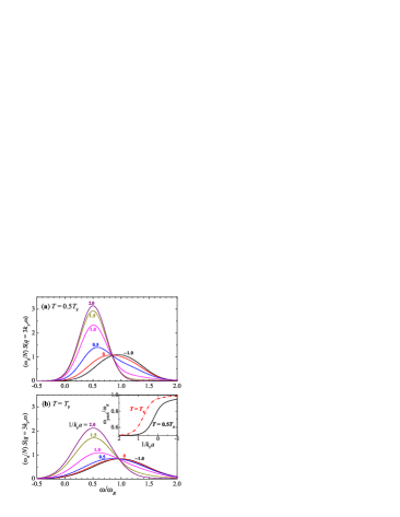
Figure 1: (Color online). Evolution of the density structure factor with increasing interaction strength $1/k_{F}a$ at $T=0.5T_{F}$ (a) and $T=T_{F}$ (b). The inset in (b) shows the peak position as a function of $1/k_{F}a$.

To understand the intermediate regime, in Fig. 1 we report numerical results for the total dynamic structure factor as the interaction strength increases from the BCS to BEC regimes. In a trapped gas with total number of fermions $N$, we use the zero temperature Thomas-Fermi wave vector $k_{F}=(24N)^{1/6}/a_{ho}$ and temperature $T_{F}=(3N)^{1/3}\hbar\omega_{0}/k_{B}$ as characteristic units. In accord with the experiment swinexpt , we take a large transferred momentum of $\hbar q=3\hbar k_{F}$. A smooth transition from atomic to molecular responses is evident as the interaction parameter $1/k_{F}a$ increases, in qualitative agreement with the experimental observation (c.f. Fig. 2 in swinexpt ). As shown in the inset, the transition shifts to the BEC side with increasing temperature.

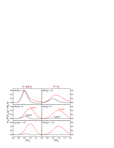
Figure 2: (Color online). $S_{\uparrow\uparrow}({\bf q},\omega)$ (dashed lines) and $S_{\uparrow\downarrow}({\bf q},\omega)$ (solid lines) at different interaction strengths and at $T=0.5T_{F}$ (left column) and $T=T_{F}$ (right column).

According to Eq. (6), the molecular response in $\Delta S_{\uparrow\uparrow,2}$ and $\Delta S_{\uparrow\downarrow,2}$ should have the same order of magnitude. However, the response is less obvious in the spin-parallel channel because of the non-interacting background in $S_{\uparrow\uparrow}({\bf q},\omega)$. As a result, $S_{\uparrow\downarrow}({\bf q},\omega)\simeq z^{2}\Delta S_{\uparrow\downarrow,2}$ provides an ideal probe for the formation of molecules. Experimentally, $S_{\uparrow\downarrow}({\bf q},\omega)$ can be measured by a proper choice of the detuning of the laser beams that results in different couplings to the two spin components combescot . In Fig. 2, we show the evolution of $S_{\sigma\sigma^{\prime}}({\bf q},\omega)$ with increasing interaction strength (from bottom to top). At lower temperatures (left column), $S_{\uparrow\downarrow}({\bf q},\omega)$ grows and becomes comparable to $S_{\uparrow\uparrow}({\bf q},\omega)$ at $1/k_{F}a=1.0$. It should be noted that our results at $T=0.5T_{F}$ are qualitatively reliable and are presented for illustrative purposes only. We expect the predictions at $T=T_{F}$ to be more quantitative, as estimated conservatively from the virial expansion of the equation of states for a trapped strongly interacting Fermi gas unitaritycmp .

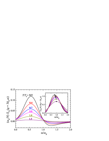
Figure 3: (Color online). Temperature dependence of $S_{\uparrow\downarrow}({\bf q},\omega)$ at unitarity. The inset shows the red shift of the total dynamic structure factor with decreasing temperature.

Fig. 3 gives the temperature dependence of the DSF at unitarity. As expected, $S_{\uparrow\downarrow}({\bf q},\omega)$ increases rapidly with decreasing temperature. As a consequence, the peak of total dynamic structure factor shifts towards the molecular recoil frequency, as indicated in the inset. This red-shift of atomic peak was indeed observed experimentally for a unitarity Fermi gas at $T\simeq 0.4T_{F}$ private .

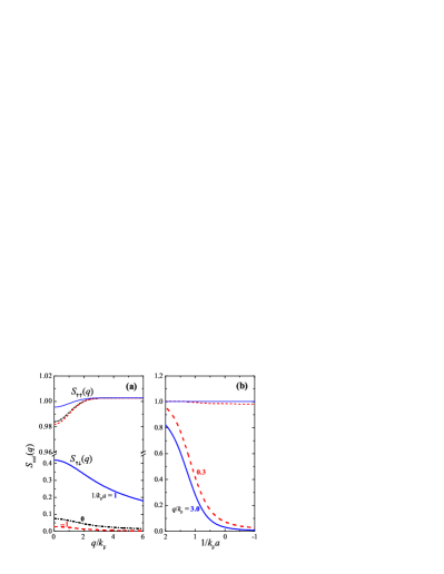
Figure 4: (Color online). Dependence of static structure factors on the momentum (a) and interaction strength (b) at $T=T_{F}$.

We have so far restricted ourselves to cases with large $q$. The momentum dependence can be conveniently illustrated by the static structure factor $S_{\sigma\sigma^{\prime}}({\bf q})=(2/N)\int d\omega S_{\sigma\sigma^{\prime}}({\bf q},\omega)$. In Fig. 4, we present $S_{\sigma\sigma^{\prime}}({\bf q})$ as a function of momentum (Fig. 4a) and interaction strength (Fig. 4b) at the Fermi temperature $T_{F}$. The spin-antiparallel structure factor depends strongly on momentum and interaction strength. In contrast, the spin-parallel structure is nearly always unity, partly due to the autocorrelations among identical spins. To better understand this, we consider the short-range behaivor of the spin-parallel structure factor in real space, $S_{\sigma\sigma}\left(\mathbf{{r}},\mathbf{r}^{\prime}\right)\equiv(2/N)\left\langle\hat{n}_{\sigma}\left({\bf r}\right)\hat{n}_{\sigma}\left({\bf r}^{\prime}\right)\right\rangle$. For parallel spins, there is no singularity as $\mathbf{r}^{\prime}\rightarrow\mathbf{r}$. Thus, to a good approximation $S_{\sigma\sigma}\left(\mathbf{{r}},\mathbf{r}^{\prime}\right)\simeq(2/N)\left\langle\hat{n}_{\sigma}\left({\bf r}\right)\right\rangle\delta\left(\mathbf{r}-\mathbf{r}^{\prime}\right)$, where the delta function comes from the anticommutator of fermion operators. After the Fourier transformation and average over the trap, we obtain $S_{\sigma\sigma}({\bf q})\simeq 1$.

IV Conclusions

In conclusion, we have developed a quantum virial expansion for dynamical properties of strongly correlated systems and have computed the dynamic density response of a strongly interacting Fermi gas at temperatures $T\sim T_{F}$. The experimentally observed transition from atomic to molecular response at low temperatures ($\sim 0.1T_{F}$) has been reproduced at a qualitative level. We anticipate that future Bragg spectroscopy at high temperatures will lead to a quantitative agreement. Alternatively, by including higher-order virial expansion functions, we may extend the validity of our results closer to the characteristic critical temperature $\sim 0.2T_{F}$ unitaritycmp . We emphasize that our virial theory is efficient for investigating other basic dynamical properties, such as the spectral function of single-particle Green function. In this respect, it may shed light on solving the paradox of the pseudogap phenomenon at unitarity akw . We leave this possibility in a future publication.

References

• (1) A. Griffin, Excitations in a Bose-Condensed Liquid (Cambridge, New York, 1993).
• (2) G. Veeravalli, E. Kuhnle, P. Dyke, and C. J. Vale, Phys. Rev. Lett. 101, 250403 (2008).
• (3) D. M. Stamper-Kurn, A. P. Chikkatur, A. Görlitz, S. Inouye, S. Gupta, D. E. Pritchard, and W. Ketterle, Phys. Rev. Lett. 83, 2876 (1999).
• (4) R. Combescot, S. Giorgini, and S. Stringari, Europhys. Lett. 75, 695 (2006).
• (5) A. Minguzzi, G. Ferrari, and Y. Castin, Eur. Phys. J. D 17, 49 (2001).
• (6) C. Chin, M. Bartenstein, A. Altmeyer, S. Riedl, S. Jochim, J. Hecker Denschlag, and R. Grimm, Science 305, 1128 (2003).
• (7) C. H. Schunck, Y. Shin, A. Schirotzek, M. W. Zwierlein, and W. Ketterle, Science 316 , 867 (2007).
• (8) A. Schirotzek, C.-H. Wu, A. Sommer, and M. W. Zwierlein, Phys. Rev. Lett. 102, 230402 (2009).
• (9) K. Miyazaki and I. M. de Schepper, Phys. Rev. E 63, 060201R ( 2001).
• (10) T.-L. Ho and E. J. Mueller, Phys. Rev. Lett. 92, 160404 (2004).
• (11) X.-J. Liu, H. Hu, and P. D. Drummond, Phys. Rev. Lett. 102, 160401 (2009).
• (12) H. Hu, X.-J. Liu, and P. D. Drummond, arXiv:1001.2085v1 (2010).
• (13) S. Nascimbène, N. Navon, K. J. Jiang, F. Chevy, and C. Salomon, Nature 463, 1057 (2010).
• (14) C. J. Vale, private communication (2009).
• (15) J. T. Stewart, J. P. Gaebler, and D. S. Jin, Nature 454, 744 (2008).