Equivalence between free and harmonically trapped quantum particles

Abstract

It is shown that general solutions of the free-particle Schrödinger equation can be mapped onto solutions of the Schrödinger equation for the harmonic oscillator. This is done in such a way that the time evolution of a free particle subjected to a sudden transition to a harmonic potential can be described by a simple coordinate transformation applied at the transition time. This procedure is computationally more efficient than either state-projection or propagator techniques. A concatenation of the map and its inverse allows us to map from one harmonic oscillator to another with a different spring constant.

I Introduction

It is known that laser beam modes in the paraxial approximation are equivalent to the eigenmodes of the harmonic oscillator Nienhuis and Allen (1993); Steuernagel (2005). The corresponding (one-dimensional, scalar) wave equation

$${\frac{\partial^{2}}{\partial x^{2}}}\theta\left(x,z\right)+i\alpha\,{\frac{\partial}{\partial z}}\theta\left(x,z\right)=0$$ (1)

arises as an approximation to Maxwell’s equations Haus (2000). In this optical context the parameter $\alpha=4\pi/\lambda$ is proportional to the (stationary, monochromatic beam’s) wave number or inversely proportional to the light’s wavelength $\lambda$.

The Schrödinger equation for a free particle in one spatial dimension $x$ is given by

$${\frac{\partial^{2}}{\partial x^{2}}}\phi\left(x,t\right)+i\alpha\,{\frac{\partial}{\partial t}}\phi\left(x,t\right)=0$$ (2)

where the parameter $\alpha=2M/\hbar$ contains the particle mass $M$ and Planck’s constant $h$, namely $\hbar=h/(2\pi)$. It is obviously equivalent to eq. (1) above.

Since the wave functions for free particles and those subjected to harmonic potentials factorize with respect to their spatial coordinates we will only discuss the one-dimensional case.

It has recently been realized that a simple coordinate transformation Steuernagel (2005) maps paraxial beams onto two-dimensional harmonic oscillator wave functions. Clearly, the same coordinate transformation can be used for the mapping of a free onto a harmonically trapped particle; in a more general setting this was noted before Takagi (1990); Bluman and Shtelen (1996). This case has added meaning since a non-adiabatic physical transition constitutes an experimentally implementable sequence of changing environmental conditions. It turns out that modelling such a transition using the standard eigenstate-projection or quantum propagator techniques is more cumbersome. State projection typically leads to infinite sums over eigenfunctions which have to be truncated and are difficult to simplify, propagator techniques involve non-trivial integrals. The results reported here may therefore not only be of fundamental but also of technical interest.

It is noteworthy that the discontinuities of the mapping of the time-coordinate in eq. (3) maps from a Schrödinger equation with a continuous to another with a discrete energy spectrum.

II Maps

II.1 Map from free to trapped case

The coordinate transformations Takagi (1990)

$$x(\xi,\tau)=\frac{\xi\sqrt{b\;\omega}}{\cos(\tau\omega)}\quad\mbox{and}\quad t(\tau)=b\tan(\tau\omega)\;,$$ (3)

applied to the wave function mapping

$$\psi(\xi,\tau) = \frac{\phi(x(\xi,\tau),t(\tau))}{f(x(\xi,\tau),t(\tau);b)},$$ (4)

$$\mbox{where}\quad f(x,t;b) = \frac{\exp\left({\frac{i\alpha tx^{2}}{4(t^{2}+b^{2})}}\right)}{(1+t^{2}/b^{2})^{1/4}},$$ (5)

yield the solution $\psi(\xi,\tau)$ for the Schrödinger equation

$$-{\frac{\partial^{2}}{\partial\xi^{2}}}\psi\left(\xi,\tau\right)+i\alpha\,{\frac{\partial}{\partial\tau}}\psi\left(\xi,\tau\right)+\frac{k\alpha}{2\hbar}\xi^{2}\psi\left(\xi,\tau\right)=0$$ (6)

of a harmonic oscillator with mass $M$, spring constant $k$ and resonance frequency $\omega=\sqrt{k/M}$.

Although this transformation maps $t\in[-\infty,\infty]$ onto $\tau\in(-\pi/2,\pi/2)$, compare with the Gouy-phase of optics Steuernagel (2005), the periodicity arising through the use of trigonometric functions meaningfully represents the oscillator’s motion for all times $\tau$.

In beam optics the confocal parameter $b$ Pampaloni and Enderlein (2004) parameterizes the strength of the beam’s focussing and the curvature of its hyperbolic flow lines Steuernagel (2005). Here, it serves as a rescaling parameter of the transverse coordinate transformation and thus allows us to stretch or squeeze the width of the wave packet we want to map.

In order to preserve the wave function normalization we have to determine the spatial coordinate stretching at the mapping time $t_{0}=\tau_{0}=0$. This yields the normalization factor ${\cal{N}}=(b\;\omega)^{1/4}$ which the wave function has to be multiplied with. The specific choice

$$b_{1}=1/\omega=\sqrt{M/k}$$ (7)

yields the natural mapping $x=\xi$ and ${\cal{N}}=1$ which we will use from now on.

II.2 Inverse map (trapped to free)

The inverse to the coordinate transformations (3) are

$$\xi = \frac{x}{\sqrt{\left(1+\omega^{2}t^{2}\right)}}$$ (8)

$$\mbox{and}\qquad\tau = \frac{1}{\omega}\arctan\left(\omega t\right)\;,$$ (9)

and go together with the wave function multiplication $\phi=\psi f$, inverting eq. (4).

II.3 Concatenated maps (trapped to trapped)

The concatenated coordinate transformations from an initial harmonic trapping potential with spring constant $k$ and wave function $\psi(\xi,\tau;k)$, via the free particle-case $\phi$, to a final harmonic potential with spring constant $K$ and wave function $\Psi(\xi,\tau;k,K)$ is given by

$$\Xi = \frac{\xi}{\sqrt{\cos^{2}(\Omega\tau)+\frac{k}{K}\sin^{2}(\Omega\tau)}}\;,$$ (10)

$$T = \frac{1}{\omega}\arctan\left(\sqrt{\frac{k}{K}}\tan\left(\Omega\tau\right)\right),\qquad$$ (11)

$$\mbox{and}\quad\Psi(\xi,\tau;k,K) = \psi(\Xi(\xi,\tau),T(\tau))$$

$$\times\frac{f(x(\xi,\tau),t(\tau);\frac{1}{\omega})}{f(x(\xi,\tau),t(\tau);\frac{1}{\Omega})}.\quad$$

Here $\Omega=\sqrt{K/M}$, and $\Psi(\xi,\tau;k,K)$ solves Schrödinger eq. (6) with $k$ substituted by $K$.

As expected for a map from one harmonic oscillator to another, the inverse of the coordinate transformations (10) and (11) are given by the same functional expressions with the quantities pertaining to one potential swapped with those of the other ($k\leftrightarrow K$ and $\omega\leftrightarrow\Omega$).

III An Example

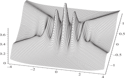
Figure 1: Probability density $P(x,t)\sim|\phi_{0}(x,t;0,p_{0})+\phi_{0}(x,t;0,-p_{0})|^{2}$ of a free quantum particle in an equal superposition of two Gaussian states as described by eq. (13)), with $\hbar=1$, $M=1$, $\sigma_{0}=3/2$, $x_{0}=0$, and opposing momenta $p_{0}=4$. The motion of the two half waves leads to interference at the origin.

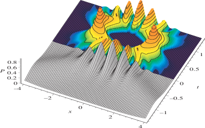
Figure 2: Probability density $P(x,t)$ of an initially free quantum particle which at time $t=\tau=0$ has the same state as the free particle displayed in Fig. 1 and suddenly gets trapped by a potential with spring constant $k=5$. This plot illustrates that the trapped particle is in a superposition state of two squeezed coherent states.

A well-known textbook example is the freely evolving Gaussian wave-packet with initial position spread $\sigma_{0}$

$$\phi_{0}(x,t;x_{0},p_{0}) = \frac{1}{\sqrt{\sqrt{\pi}\sigma(t)}}\exp{\left[{{\frac{v_{0}\,\left(x_{0}\,\hbar\,t-iM\sigma_{0}^{2}x\right)}{\hbar\sigma_{0}\sigma(t)}}}\right]}$$ (13)

$$\times \exp{\left[{-\frac{\left(x-x_{0}\right)^{2}}{2\sigma_{0}\sigma(t)}}-{\frac{i\sigma_{0}\,M{v_{0}}^{2}t}{2\hbar\sigma(t)}}\right]},$$

$$\mbox{where}\quad\sigma(t) = \sigma_{0}+i\frac{t\hbar}{\sigma_{0}M}.$$ (14)

Here $x_{0}$ parameterizes spatial, and $p_{0}=Mv_{0}$ momentum displacement of the wave functions. If either of these two quantities is non-zero the mapping onto a harmonically trapped state results in a state with oscillating center-of-mass. In general, although a wave function of Gaussian shape, this freely evolving wave packet will also not ‘fit’ the width of the harmonic potential and therefore be squeezed. In short, the state of eq. (13) trapped in a harmonic potential becomes a squeezed coherent state Schleich (2001). For a superposition of such states see Fig. 1 and for this superposition state being trapped consult Fig. 2.

IV Conclusion

It is shown that general solutions of the free-particle Schrödinger equation can be mapped onto solutions of the Schrödinger equation for the harmonic oscillator using a simple coordinate transformation in conjunction with a multiplication of the wave function by a suitable phase factor. This map is invertible and a concatenation of two such maps allows us to map from one harmonic oscillator to another with a different spring constant. The simplicity of the approach described here makes it a tool of choice for the description of the wave function of a particle experiencing instantaneous transitions from a free to a harmonically trapped state, the sudden release from a harmonic trap, or the sudden change of the strength of its harmonic trapping potential.

The mapping introduced here is computationally more efficient than state-projection or propagator techniques and conceptually simpler than mapping techniques such as those used for supersymmetric potentials Gendenshteïn (1983); Cooper et al. (1989). It may even help with numerical calculations because it allows for the determination of the behaviour of wave functions trapped in a harmonic potential using the lower computational overheads of wave functions in free space.

References

- Nienhuis and Allen (1993) G. Nienhuis and L. Allen, Phys. Rev. A 48, 656 (1993).
- Steuernagel (2005) O. Steuernagel, Am. J. Phys. 73, 625 (2005), eprint arXiv:physics/0312116v2.
- Haus (2000) H. A. Haus, Electromagnetic Noise and Quantum Optical Measurements (Springer, Heidelberg, 2000).
- Takagi (1990) S. Takagi, Prog. Theor. Phys. 84, 1019 (1990).
- Bluman and Shtelen (1996) G. Bluman and V. Shtelen, J. Phys. A: Math. Gen. 29, 4473 (1996).
- Pampaloni and Enderlein (2004) F. Pampaloni and J. Enderlein (2004), eprint arXiv:physics/0410021.
- Schleich (2001) W. P. Schleich, Quantum Optics in Phase Space (Wiley-VCH, Berlin, 2001).
- Gendenshteïn (1983) L. É. Gendenshteïn, Sov. J. Exp. Theor. Phys. Lett. 38, 356 (1983).
- Cooper et al. (1989) F. Cooper, J. N. Ginocchio, and A. Wipf, J. Phys. A: Math. Gen. 22, 3707 (1989).