Efficient Automation of Index Pairs in Computational Conley Index Theory

Abstract.

We present new methods of automating the construction of index pairs, essential ingredients of discrete Conley index theory. These new algorithms are further steps in the direction of automating computer-assisted proofs of semi-conjugacies from a map on a manifold to a subshift of finite type. We apply these new algorithms to the standard map at different values of the perturbative parameter $\varepsilon$ and obtain rigorous lower bounds for its topological entropy for $\varepsilon\in[.7,2]$.

1. Introduction

The literature on computer-assisted proofs in dynamical systems through topological methods involves, for the most part, the investigation of the mapping properties of certain compact sets which go under different names in different settings: they are called index pairs in Conley index theory and windows or h-sets in the theory of correctly aligned windows or covering relations [ZG04], which are the two leading theories applied in topological, computer-assisted proofs in dynamical systems. An index pair is not necessarily an h-set and vice-versa, but they both satisfy the crucial property that they map across themselves in a way similar to the way Smale’s horseshoe maps across itself. In other words, they agree in some sense with the expanding and contracting directions of the map and thus they can be thought of as slight generalizations of Markov partitions. Not surprisingly, after several conditions are met in each setting, one is able to prove a semi-conjugacy to symbolic dynamics, giving a good description the dynamics of a large set of the orbits of a dynamical system, much like one can give a good description of the dynamics of Smale’s horseshoe via the easily-describable dynamics of the full 2-shift. Given an index pair, an automated procedure was described in [DFT08] to prove a semi-conjugacy to a sub-shift of finite type (SFT).

The first major push towards automated validation and automated computer-assisted proofs using topological methods can be found in [DJM05]. By validation we mean a mechanism which upholds the claim of a theorem in rigorous way by means of finitely many calculations on a computer. Built on those and other results, [DFT08] achieved the complete automation of the validation part of a computer-assisted proof. In this paper we address the issue of automating the creation of index pairs in a computationally efficient way.

There are many reasons why automated proof techniques such as [DFT08] come at an advantage. For example, for parameter-depending systems, automation allows for the rigorous exploration of a system at many parameters. Such applications of [DFT08] have already been carried out in [Fro10]. Besides exploration at different values of parameters, automated methods may permit us to construct index pairs where it would be otherwise impossible to do so by hand. In [DFT08] computer-assisted proofs were given of a semi-conjugacy from the classical Hénon map to a SFT with 247 symbols. These proofs were completely automated, that is, besides an input of initial parameters, there was no human intervention from start to finish in the computation which proved the semi-conjugacy and bounded the topological entropy.

It should be noted that the complete automation described in the previous paragraph is remarkable. To prove a semi-conjugacy using topological methods on a computer the following steps must be taken:

1. Locate and identify the relevant invariant objects;

2. construct a compact set $K$ (refered to above, in our case the index pair) whose components map onto each other in a way which is compatible with the dynamics of the system;

3. prove that some of the dynamics of the system can be described via the mapping properties between the components of $K$.

Each of these steps presents its own challenges and difficulties. In [DFT08, §3.2] step (3) was completely solved, in the sense that given any compact set (index pair) $K$ which satisfies the properties required by (2), a completely automated routine was given to prove a semi-conjugacy. Steps (1) and (2), the creation of the index pair, were also fully automated in [DFT08, §3.1] (and [Fro10]), largely due to the properties of “well-behaved” maps like the Hénon map: it has a low-dimensional attractor and all its periodic orbits exhibit hyperbolic-like behavior from a computational perspective. In other words, in such cases there is a dominating invariant set, namely the attractor whose periodic orbits all seem hyperbolic and are easily localizable. Thus, it is of interest to consider the case where we do not have such underlying structure. Quoting directly from [DFT08, §5]: “… further analysis and optimization of the procedure described in section 3.1 for locating a region of interest should lead to even stronger results.”

This article is an effort to extend the methods and techniques presented in [DFT08] to more general situations with the aim of dealing with systems which do not exhibit Hénon-like behavior. As an illustration of the approach we propose, we apply our method to the standard map

$$f_{\varepsilon}:(x,y)\mapsto\left(x+y+\frac{\varepsilon}{2\pi}\sin(2\pi x)\mbox{ mod 1 },y+\frac{\varepsilon}{2\pi}\sin(2\pi x)\mbox{ mod 1 }\right),$$

for $(x,y)\in S^{1}\times S^{1}=\mathbb{T}^{1}$, at different values of the perturbation parameter $\varepsilon$. By treating the perturbation parameter as an interval, we are also able to give a description of the orbits of the map in terms of symbolic dynamics for all perturbation values inside the given interval. We chose the standard map for a couple of reasons. First, it is a very well-known system with rich dynamics. Second, in contrast with previous results for Hénon-like systems (e.g. [DFT08, Fro10]), the standard map is a volume-preserving map which exhibits both hyperbolic and elliptic behavior, which make the task of automating the construction of index pairs considerably more difficult. Finally, we generalize the methods of [DFT08] to work on manifolds with nontrivial topologies and not just $\mathbb{R}^{n}$, and our application to the standard map exemplifies this.

In the present constructions, we benefit much from some a-priori information of the map. The distinction between a hyperbolic or elliptic periodic orbit, for example, is a crucial one. Symmetries of the map, the knowledge of the precise location of any heteroclinic or homoclinic orbits are also valuable data from which to begin. In our view, a little previous knowledge goes a long way, as we exploit this a-priori information to make the constructions highly efficient while keeping the entire process highly automated.

We mention that besides [DFT08] there have been other recent efforts towards the automation of computer-assisted proofs in dynamical systems. In particular, [MJ09] is a collection of set-oriented algorithms for the creation of index pairs adapted for volume-preserving maps. In addition, [BCG07, BCGH08] use the method of covering relations after reducing the problem of finding suitable sets and maps between sets to a problem of global optimization theory.

In contrast to other Conley index methods [DFT08, MJ09] which are top-down, in that they start with a large portion of the phase space and try to narrow down to the invariant objects, our method is bottom-up, in that we are guided by the dynamics of the system as we “grow out” the index pairs given good numerical approximations of the invariant sets (see Algorithms 2 and 3). The goal of our bottom-up approach is to compute a minimal number of images of a discretized version of the map (see section 2.3), which is often the most expensive part of computations. Our approach thus achieves high efficiency in the automation of the construction of an index pair.

The present work has been motivated by the challenges brought by the standard map to the task of automating the construction of index pairs and by what we expect will be obstacles for construction of index pairs in future applications. The techniques of this paper along with those of [DFT08] and the references therein provide a solid set of tools for automating computer assisted proofs in the paradigm of planar maps with positive entropy through discrete Conley index theory. These methods are technically not restricted to dimension 2, but remain mostly untested in higher dimensional examples with higher dimensional unstable bundles. To the authors’ knowledge, there is an example in [DJM04] with a two dimensional unstable bundle, but no others in the existing computational Conley index literature. Having focused on making the construction of index pairs highly efficient in this paper, it remains to apply them to such higher dimensional examples, which we plan to do in future work.

To the authors’ knowledge, the rigorous bounds presented here on the topological entropy for the standard map are the only ones of their kind in the literature. We could only find [YT09] for computational lower bounds of the topological entropy for the standard map at various parameter values, but the results there are non-rigorous. Thus it would be interesting to see how other topological methods (for example [ZG04, NBGM08]) perform for the same values we have examined in this paper.

This paper is organized as follows: in section 2 we review the necessary background for the subsequent sections. Section 3 details the data structures we use in our algorithms as well as presents the two new algorithms which we consider as the main contribution of this work, Algorithms 2 and 3. We apply these algorithms in section 4 to the standard map to give lower bounds for the topological entropy at different values of the perturbative parameter. Theorem 4.1 gives lower bounds of the topological entropy of the standard map as given by topological entropy of sub-shifts of finite type, for all $f_{\varepsilon}$ with $\varepsilon\in[0.7,2.0]$. Theorem 4.2 gives a positive lower bound for the topological entropy for $\varepsilon=\frac{1}{2}$. Theorems 4.3 and 4.4 give a positive lower bound for the topological entropy for $\varepsilon=2$ by finding connecting orbits to hyperbolic periodic orbits of higher period. We conclude with some comments and remarks on the implementation in Section 4.4.

Acknowledgements.

We would like to thank Jay James for many helpful discussions during the course of this work, as well as for his help with the implementation of the methods of [CFdlL05] for the standard map, as well as Sarah Day for helpful comments on an early draft of the paper. We also thank the Center for Applied Mathematics at Cornell University for allowing us access to their computational facilities, where the computations in this paper were carried out. We would like to thank an anonymous referee for helping us make the paper clearer.

2. Background

We review in this section the necessary facts about topological entropy, symbolic dynamics, and the discrete Conley index which will be relevant in the later sections. Although the exposition will not be in depth, we encourage the interested reader to consult section 2 of [DFT08] for a more detailed exposition. For deeper treatment of the discrete Conley index, see [MM02].

2.1. Topological Entropy and Symbolic Dynamics

Let $f:X\rightarrow X$ be a map. The topological entropy of $f$ is the quantity $h(f)\in\mathbb{R}\cup\{\infty\}$ which is a good measure of the complexity of $f$. A map with positive topological entropy usually exhibits chaotic behavior in many of its trajectories.

Definition 2.1.

Let $f:X\rightarrow X$ be a continuous map. A set $W\subset X$ is called $(n,\varepsilon)$-separated for $f$ if for any two different points $x,y\in W$, $\|f^{k}(x)-f^{k}(y)\|>\varepsilon$ for some $k$ with $0\leq k<n$. Let $s(n,\varepsilon)$ be the maximum cardinality of any $(n,\varepsilon)$-separated set. Then

$$h(f)=\sup_{\varepsilon>0}\limsup_{n\rightarrow\infty}\frac{\log s(n,\varepsilon)}{n}$$

is the topological entropy of $f$.

Although it is always well-defined, it is usually impossible to compute the topological entropy directly from the definition. The set of systems for which it is computable is rather small, but it contains all systems from symbolic dynamics.

Let $\Sigma_{N}=\{0,\dots,N-1\}^{\mathbb{Z}}$ be the set of all bi-infinite sequences on $N$ symbols. It is well-known that $\Sigma_{N}$ is a complete metric space. Define the full N-shift $\sigma:\Sigma_{N}\rightarrow\Sigma_{N}$ to be the map acting on $\Sigma_{N}$ by $(\sigma(x))_{i}=x_{i+1}$. Given an $N\times N$ matrix $A$ with $A_{i,j}\in\{0,1\}$ we can define a sub-shift of finite type defined on $\Sigma_{A}\subset\Sigma_{N}$, where $x\in\Sigma_{A}$ if and only if for $x=(\dots,x_{i},x_{i+1},\dots)$, $A_{x_{i},x_{i+1}}=1$ for all $i$. In other words, $\Sigma_{A}$ consists of all sequences in $\Sigma_{N}$ with transitions of $\sigma$ allowed by $A$. Viewed as a graph with $N$ vertices and with an edge from vertex $i$ to vertex $j$ if and only if $A_{i,j}=1$, $\Sigma_{A}$ can be identified with the set of all infinite paths in such graph.

The topological entropy of a sub-shift of finite type is computed through the largest eigenvalue of its transition matrix $A$.

Theorem 2.2.

Let $\sigma:\Sigma_{A}\rightarrow\Sigma_{A}$ be a subshift of finite type. Then its topological entropy is

$$h(\sigma)=\log\mbox{sp}(A),$$

where $\mbox{sp}(A)$ denotes the spectral radius of $A$.

In order to study a map $f$ of high complexity, it is sometimes possible to study a subsystem of it through symbolic dynamics. This is done through a semi-conjugacy.

Definition 2.3.

Let $f:X\rightarrow X$ and $g:Y\rightarrow Y$ be continuous maps. A semi-conjugacy from $f$ to $g$ is a continuous surjection $h:X\rightarrow Y$ with $h\circ f=g\circ h$. We say $f$ is semi-conjugate to $g$ if there exists a semi-conjugacy.

Note that through a semi-conjugacy $h:X\rightarrow Y$, information about $g$ acting on $Y$ gives information about $f$ acting on $x$. In particular, the topological entropy of $g$ bounds from below the topological entropy of $f$.

Theorem 2.4.

Let $f$ be semi-conjugate to $g$. Then $h(f)\geq h(g)$.

Corollary 2.5.

Let $f$ be semi-conjugate to $\sigma:\Sigma_{A}\rightarrow\Sigma_{A}$, for some $N\times N$ matrix $A$. Then

$$h(f)\geq\mbox{sp}(A).$$

2.2. The Discrete Conley Index

Let $f:M\rightarrow M$ be a continuous map, where $M$ is a smooth, orientable manifold.

Definition 2.6.

A compact set $K\subset M$ is an isolating neighborhood if

$$\mbox{Inv}(K,f)\subset\mbox{Int}(K),$$

where $\mbox{Inv}(K,f)$ denotes the maximal invariant set of $K$ and $\mbox{Int}(K)$ denotes the interior of $K$. $S$ is an isolated invariant set if $S=\mbox{Inv}(K,f)$ for some isolating neighborhood $K$.

Definition 2.7 ( [RS88]).

Let $S$ be an isolated invariant set for $f$. Then $P=(P_{1},P_{0})$ is an index pair for $S$ if

1. $\overline{P_{1}\backslash P_{0}}$ is an isolating neighborhood for $S$.

2. The induced map

   $$f_{P}(x)=\left\{\begin{array}[]{ll}f(x)&\mbox{ if $x$, $f(x)\in P_{1}/P_{0}$ },\\ \mbox{$[P_{0}]$}&\mbox{ otherwise}.\end{array}\right.$$

   defined on the pointed space $(P_{1}/P_{0},[P_{0}])$ is continuous.

Definition 2.8 ( [Wil70]).

Let $G,H$ be abelian groups and $\varphi:G\rightarrow G$, $\psi:H\rightarrow H$ homomorphisms. Then $\varphi$ and $\psi$ are shift equivalent if there exist homomorphisms $r:G\rightarrow H$ and $s:H\rightarrow G$ and a constant $k\in\mathbb{N}$ such that

$$r\circ\varphi=\psi\circ r,\;\;s\circ\psi=\varphi\circ s,\;\;r\circ s=\psi^{k},\;\;\mbox{ and }s\circ r=\varphi^{k}.$$

Shift equivalence defines an equivalence relation, and we denote by $[\varphi]_{s}$ the class of all homomorphisms which are shift equivalent to $\varphi$.

Definition 2.9 ( [FR00]).

Let $P=(P_{1},P_{0})$ be an index pair for an isolated invariant set $S=\mbox{Inv}(\overline{P_{1}\backslash P_{0}},f)$ and let $f_{P*}:H_{*}(P_{1},P_{0};\mathbb{Z})\rightarrow H_{*}(P_{1},P_{0};\mathbb{Z})$ be the map induced by $f_{P}$ on the relative homology groups $H_{*}(P_{1},P_{0};\mathbb{Z})$. The Conley index of $S$ is the shift equivalence class $[f_{P*}]_{s}$ of $f_{P*}$.

One can think of two maps $f_{P*}$ and $g_{\bar{P}*}$ as being in the same shift equivalence class if and only if they have the same assymptotic behavior. Since an index pair for an isolated invariant set is not unique, the Conley index of and isolated invariant set does not depend on the choice of index pair. There are two elementary yet important results which link the Conley index of an isolated invariant set with the dynamics of $f$. The first one is the so-called Ważewski property:

Theorem 2.10.

If $[f_{P*}]_{s}\neq[0]_{s}$, then $S\neq\varnothing$.

Since similar assymptotic behavior relates two different maps in the same shift equivalence class, it is sufficient then to have a map $f_{P*}$ not be nilpotent in order to have a non-empty isolated invariant set. In practice, non-nilpotency can be verified by taking iterates of a representative of $[f_{P*}]_{s}$ until non-nilpotent behavior is detected. We also have an elementary detection method of periodic points.

Theorem 2.11 (Lefshetz Fixed Point Theorem).

Let $f_{*}$ be a representative of $[f_{P*}]_{s}$ with maps $f_{k}:H_{k}(P_{1},P_{0};\mathbb{Z})\rightarrow H_{k}(P_{1},P_{0};\mathbb{Z})$ which are represented by matrices. Then if

$$\Lambda(f_{*})=\sum_{k\geq 0}(-1)^{k}\mbox{ tr }f_{k}\neq 0,$$

then $f$ has a fixed point. Moreover, if $\Lambda(f_{*}^{n})\neq 0$, then $f$ has a periodic point of period $n$.

Since traces are preserved under shift equivalence, $\Lambda(f_{*})$ is independent of the representative of $[f_{P*}]_{s}$, and we may even denote it as $\Lambda([f_{P*}]_{s})$.

Corollary 2.12.

Let $K\subset M$ be the finite union of disjoint, compact sets $K_{1},\dots,K_{m}$ and let $S=\mbox{Inv}(K,f)$. Let $S^{\prime}=\mbox{Inv}(K_{1},f_{K_{m}}\circ\cdots\circ f_{K_{1}})\subset S$ where $f_{K_{i}}$ denotes the restriction of $f$ to $K_{i}$. If

$$\Lambda([f_{K_{m}}\circ\cdots\circ f_{K_{1}}]_{s})\neq 0$$

then $f_{K_{m}}\circ\cdots\circ f_{K_{1}}$ contains a fixed point in $S^{\prime}$ which corresponds to a periodic orbit of $f$ which travels through $K_{1},\dots,K_{m}$ in such order.

This is a strong and useful tool for proving the existence of periodic orbits. However, we may have $\Lambda([f_{K_{m}}\circ\cdots\circ f_{K_{1}}]_{s})=0$ while $(f_{K_{m}}\circ\cdots\circ f_{K_{1}})_{*}$ is not nilpotent and thus have an invariant set which may be of interest since it behaves like a periodic orbit. So we have an analogous result based on the Ważewski property.

Corollary 2.13.

Let $K\subset M$ be the finite union of disjoint, compact sets $K_{1},\dots,K_{m}$ and let $S=\mbox{Inv}(K,f)$. Let $S^{\prime}=\mbox{Inv}(K_{1},f_{K_{m}}\circ\cdots\circ f_{K_{1}})\subset S$ where $f_{K_{i}}$ denotes the restriction of $f$ to $K_{i}$. If

$$[(f_{K_{m}}\circ\cdots\circ f_{K_{1}})_{*}]_{s}\neq[0]_{s},$$

then $S^{\prime}$ is nonempty. Moreover, there is a point in $S$ whose trajectory visits the sets $K_{i}$ in such order.

Both corollaries can be useful in different settings when used to to prove symbolic dynamics through computer-assistance. When existence of periodic points is of primary concern, one can use Corollary 2.12. When existence of trajectories which shadow a certain prescribed path given by a symbol sequence, but that do not necessarily correspond to periodic orbits, Corollary 2.13 is the better tool. This may occur when there are higher-dimensional invariant sets to which the restriction of the dynamics is quasi-periodic. In either case, what makes the implementation possible is the ease of computability of the traces of the induced maps on homology for Corollary 2.12 and a sufficient condition for non-nilpotency in the case of Corollary 2.13. For more details on the implementation, see [DFT08].

2.3. Combinatorial Structures

All concepts from the discrete Conley index theory from the previous section have analogous definitions in a combinatorial setting for which computer algorithms can be written.

Definition 2.14.

A multivalued map $F:X\rightrightarrows X$ is a map from $X$ to its power set, that is, $F(x)\subset X$. If for some continuous, single-valued map $f$ we have $f(x)\in F(x)$ and $F$ is acyclic, then $F$ is an enclosure of $f$.

The reason multivalued maps and enclosures are used in our computations is that if they are done properly, they give rigorous results. Moreover, if $F$ is an enclosure of $f$ and $(P_{0},P_{1})$ is an index pair for $F$ (as we will define below), then it is an index pair for $f$. It also follows that if we can compute the Conley index of $F$ and process the information encoded in it, we may obtain information about the dynamics of $f$.

We begin by setting up a grid $\mathcal{G}$ on $M$, which is a compact subset of the $n$ dimentional manifold $M$ composed of finitely many elements $\mathcal{B}_{i}$. Each element is a cubical complex, hence a compact set, and it is essentially an element of a finite partition of a compact subset of $M$. In practice, all elements of the grid are rectangles represented as products of intervals (viewed in some nice coordinate chart), that is, for $\mathcal{B}_{i}\in\mathcal{G}$, $\mathcal{B}_{i}=\prod_{k=1}^{n}[x^{i}_{k},y^{i}_{k}]$. We refer to each element of $\mathcal{G}$ as a box and each box is defined by its center and radius, i.e., $\mathcal{B}_{i}=(c_{i},r_{i})$, where $c_{i}$ and $r_{i}$ are $n$-vectors with entries corresponding to the center and radius, respectively, in each coordinate direction. In practice we have $r_{i}$ the same for all boxes in $\mathcal{G}$ but this is in no way necessary and there may be systems for which variable radii for boxes provide a significant advantage. For a collection of boxes $\mathcal{K}\subset\mathcal{G}$, we denote by $|\mathcal{K}|$ its topological realization, that is, its corresponding subset of $M$. From now on we will use caligraphy capital letters to denote collections of boxes in $\mathcal{G}$ and by regular capital letters we will denote their topological realization, e.g., $|\mathcal{B}_{i}|=B_{i}$.

The way we create a grid is as follows. We begin with with one big box $\mathcal{B}$ such that $|\mathcal{B}|$ encloses the area we wish to study. Then we subdivide $\mathcal{B}$ $d$ times in each coordinate direction in order to increase the resolution at which the dynamics are studied. The integer $d$ will be refered to as the depth. Thus working at depth $d$ gives us a maximum of $2^{dn}$ ($n=\dim M$) boxes with which to work of each coordinate of size $2^{-d}$ relative to the original size of the box $\mathcal{B}$.

Definition 2.15.

A combinatorial enclosure of $f$ is a multivalued map $\mathcal{F}:\mathcal{G}\rightrightarrows\mathcal{G}$ defined by

$$\mathcal{F}(\mathcal{B})=\{\mathcal{B}^{\prime}\in\mathcal{G}:|\mathcal{B}^{\prime}|\cap F(B)\neq\varnothing\},$$

where $F$ is an enclosure of $f$.

In practice, combinatorial enclosures are created as follows. One begins with $\mathcal{B}\in\mathcal{G}$ and defines $F(x)$, $x\in B=|\mathcal{B}|$, as the image of $B$ using a rigorous enclosure for the map $f$. Rigorous enclosures are obtained by keeping track of the error terms in the computations of the image of a box and making sure the true image $f(B)$ is contained in $|\mathcal{F}(\mathcal{B})|$. In this paper, all rigorous enclosures will be obtained with the use of interval arithmetic using Intlab [Rum99]. Note that $|\mathcal{F}|$ becomes an enclosure of $f$. $\mathcal{F}:\mathcal{G}\rightrightarrows\mathcal{G}$ can also be represented as a matrix $\mathcal{T}$ with entries in $\{0,1\}$ with $\mathcal{T}_{i,j}=1$ if and only if $\mathcal{B}_{j}\in\mathcal{F}(\mathcal{B}_{i})$. Moreover $\mathcal{T}$ can be viewed as a directed graph with vertices corresponding to individual boxes in $\mathcal{G}$ and edges going from box $i$ to box $j$ if and only if $\mathcal{T}_{i,j}=1$.

Definition 2.16.

A combinatorial trajectory of a combinatorial enclosure $\mathcal{F}$ through $\mathcal{B}\in\mathcal{G}$ is a bi-infinite sequence $\gamma_{G}=(\dots,\mathcal{B}_{-1},\mathcal{B}_{0},\mathcal{B}_{1},\dots)$ with $\mathcal{B}_{0}=\mathcal{B}$, $\mathcal{B}_{n}\in\mathcal{G}$, and $\mathcal{B}_{n+1}\in\mathcal{F}(\mathcal{B}_{n})$ for all $n\in\mathbb{Z}$.

The definitions which follow are by now standard in the computational Conley index literature. We will state definitions and refer the reader to [DFT08] for the algorithms which construct the objects defined.

Definition 2.17.

The combinatorial invariant set in $\mathcal{N}\subset\mathcal{G}$ for a combinatorial enclosure $\mathcal{F}$ is

$$\mbox{Inv}(\mathcal{N},\mathcal{F})=\{\mathcal{B}\in\mathcal{G}:\mbox{ there exits a trajectory }\gamma_{G}\subset\mathcal{N}\}.$$

Definition 2.18.

The combinatorial neighborhood or one-box beighborhood of $\mathcal{B}\subset\mathcal{G}$ is

$$o(\mathcal{B})=\{\mathcal{B}^{\prime}\in\mathcal{G}:|\mathcal{B}^{\prime}|\cap|\mathcal{B}|\neq\varnothing\}.$$

Definition 2.19.

If

$$o(\mbox{Inv}(\mathcal{N},\mathcal{F}))\subset\mathcal{N}$$

then $\mathcal{N}\subset\mathcal{G}$ is a combinatorial isolating neighborhood for $\mathcal{F}$.

A procedure for creating a combinatorial isolating neighborhood is discussed in Section 3 and an given by Algorithm 1. Once we have a combinatorial isolating neighborhood, it is possible to define and create a combinatorial index pair.

Definition 2.20.

A pair $\mathcal{P}=(\mathcal{P}_{1},\mathcal{P}_{0})\subset\mathcal{G}$ is a combinatorial index pair for the combinatorial enclosure $\mathcal{F}$ if its topological realization $P_{i}=|\mathcal{P}_{i}|$ is an index pair for any map $f$ for which $\mathcal{F}$ is an enclosure.

One of the main goals of this paper is a procedure to efficiently compute combinatorial index pairs. This is the content of the next section. We now have made all definitions necessary to define the Conley index. Computing the induced map on homology at the combinatorial level is no trivial task. We refer the enthusiastic reader to [KMM04] for a very thourough exposition on computing induced maps on homology. In practice, we use the computational package homcubes, part of the computational package CHomP [cho], which computes the necessary maps on homology to define the Conley index.

3. Automated Symbolic Dynamics

The results of [DFT08] show that it is possible to create an automated procedure to rigorously prove a semi-conjugacy from a map $f:M\rightarrow M$ to a subshift $\Sigma_{A}$. The procedure detailed in [DFT08] can be summarized as follows:

1. Start with a rectangle in $\mathbb{R}^{n}$ and obtain a grid of boxes of constant radius by partitioning it in each coordinate direction $d$ times for some fixed $d$.

2. Compute the combinatorial enclosure $\mathcal{F}$ of $f$ in a neighborhood of the area of interest, given by the interval arithmetic images of boxes in the grid. For some fixed $k$, create a collection $\mathcal{P}_{k}\subset\mathcal{G}$ of boxes which are periodic of period $n\leq k$ under $\mathcal{F}$ by finding non-zero entries of the diagonal of $\mathcal{T}^{n}$.

3. Using shortest path algorithms, and denoting by $\mathcal{D}_{ij}$ any shortest path between $\mathcal{B}_{i}\in\mathcal{P}_{k}$ and $\mathcal{B}_{j}\in\mathcal{P}_{k}$ in $\mathcal{G}$ (if there is no such path, $\mathcal{D}_{ij}=\varnothing$), create a collection $\mathcal{A}\subset\mathcal{G}$ by $\mathcal{A}=\mathcal{P}_{k}\cup\left(\bigcup_{i\neq j}\mathcal{D}_{ij}\right)$. Using the appropriate algorithms, create a combinatorial isolating neighborhood for $\mathcal{A}$, a combinatorial index pair, and compute its Conley index $[f_{P*}]_{s}$.

4. Working with a representative of $[f_{P*}]_{s}$ as matrices (one for each level of homology) over the integers, we filter out all the nilpotent behavior and find a smaller representative which exhibits only recurrent behavior.

5. We study $[f_{P*}]_{s}$ by its action on the generators of $H_{1}(P_{1},P_{0};\mathbb{Z})$ grouped by disjoint components of $P_{1}\backslash P_{0}$, and using Corollary 2.13 we perform a finite number of calculations to prove a semiconjugacy from $f$ to $\Sigma_{A}$, where $A$ is a $m\times m$ matrix, and $m$ is a number less than or equal to the number of disjoint components of $P_{1}\backslash P_{0}$.

This method was applied to the Hénon map and a semi-conjugacy to a subshift on 247 symbols was proved, which gave a rigorous lower bound on the topological entropy.

We make a few remarks about the approach. First, although all periodic orbits of the Hénon map exhibit hyperbolic behavior, this is not true in all systems. In Hamiltonian systems, for example, one expects roughly half of the periodic orbits to be isolated invariant sets. Thus looking at the diagonal of $\mathcal{T}^{n}$ is not enough to capture orbits which will give us isolated invariant sets and a nontrivial Conley index. Another issue which arises in practice is the computational complexity of the algorithms to prove a semiconjugacy to a subshift. The complexity increases exponentially with the dimension of the system and if we have any hope of getting results in systems of dimension higher than 2, we must perform the computations as efficiently as possible.

With this in mind, we view the entire process of proving a semi-conjugacy as the composition of two major steps:

1. The gathering of recurrent, isolated invariant sets. This can be done through a combination of non-rigorous numerical methods, graph algorithms, set-oriented methods, linear algebra operations, et cetera.

2. A proof that this behavior in fact exists through a semi-conjugacy to a subshift.

We point out that the second step is solved in [DFT08]. That is, given as input an index pair $(P_{0},P_{1})$ and the combinatorial enclosure $\mathcal{F}$ of $f$ used to create it, proving semi-conjugacy from $f$ to a subshift is completely automated. The first step is also largely dealt with, but the approach is not as general as it can be, as it was devised to deal with maps like the Hénon map where isolation is easy. We wish to consider cases where one cannot simply compute the map on all boxes in the area of interest, either because the dimension of the attractor is too high or because one needs a very high box resolution to achieve isolation. Whereas [DFT08] focused on (2), here we focus on (1) and on how to produce index pairs more efficiently. In settings where isolation is difficult, our methods in this paper to efficiently deal with (1) and the solution in [DFT08] of (2) constitute a better method to prove semi-conjugacies to a SFT.

We provide an efficient method of computing an index pair in step (1) when one knows roughly what to look for. In essence, we believe that a small amount of a-priori knowledge goes a long way. In other words, we can simplify and make computations much more efficient if we know something about dynamics beforehand, like previous knowledge of the location of periodic, heteroclinic, homoclinic orbits, special symmetries of the system, et cetera. We will illustrate this approach with examples in Section 4.

More precisely, we take as input a list of periodic points and pairs of points which might have connecting orbits between them, and produce an index pair containing all of the points and connections, if possible. For example, if one had numerical approximations of two fixed points and conjectured that there was a connecting orbit between them, our algorithms could potentially prove the existence of the connection.

We break the task of finding an index pair into two steps. The first is to approximate numerically the invariant objects whose existence we want to prove, and the second is to cover such an approximation with boxes and add boxes until the index pair conditions are satisfied. Before describing these steps, however, we introduce our underlying data structures.

3.1. Data Structures

The algorithms we present rely on some basic data structures to encode the topology of the phase space and the behavior of the map. We require two routines to keep track of the topology: finding the box corresponding to a particular point in the phase space (to compute the multivalued map on boxes), and determining which boxes are adjacent (to determine isolation). We then of course need a method of storing the multivalued map itself.

To accomplish all of this, we consider a subset $S$ of our grid and enumerate the boxes in $S$, giving each a unique integer. We then store the position information in a binary search tree, which we simply call the tree, so that the index $i$ for the box $b_{i}$ covering a given point $x$ in the phase space (i.e., $x\in|b_{i}|$) may be computed efficiently. We use the GAIO implementation for our basic tree data structure [DFJ01] only, and make use of some enhancements, discussed below. To encode the topology, we store the adjacency information in a (symmetric) binary matrix $Adj$, where $Adj_{\,ij}=Adj_{\,ji}=1$ if and only if boxes $b_{i}$ and $b_{j}$ are adjacent. More precisely, $Adj_{\,ij}=1$ if and only if $|b_{i}|\cap|b_{j}|\neq\varnothing$. We will call this matrix the adjacency matrix. This is a crucial component when working on spaces with nontrivial topology such as the torus, as we will see in section 4. Finally, we store the multivalued map as a transition matrix $P$ such that $P_{ji}=1$ if and only if $b_{j}\in\mathcal{F}(b_{i})$.

Below are the operations of the tree data structure:

1. $S$ = boxnums() – Return a list of all box numbers in the tree

2. $S$ = find($C$) – Given a set $C\subset M$ of points, return the indices $S$ of boxes covering any $x\in C$

3. insert($C$) – Insert boxes into the tree covering points $C\subset M$ (if they do not already exist)

4. delete($S$) – Remove boxes with indices in $S$ from the tree

5. subdivide() – For each box $b$ in the tree, divide each of its coordinate directions in half creating $2^{n}$ smaller boxes, thus increasing the depth of the tree by 1

Although the GAIO tree data structure is in many ways well-suited to our task, it has a few simple drawbacks which significantly restrict our computations. Specifically, the operations insert($\cdot$) and delete($\cdot$) scramble the box numbers of the tree as a side-effect. Thus, if we want to keep track of our current box set while inserting or deleting boxes, we have to spend extra time computing the new box numbers. Without knowledge of how the renumbering is done, this would take $O(n\log n)$ time, where $n$ is the number of boxes, since for each box we have to search the tree to find its new number. The best one could hope for would be $O(\log n)$ with careful bookkepping (one still needs logarithmic time to locate the place in the tree for insertion or deletion). We managed to compute the new box numbers in $O(n)$ time by observing that the numbering is given by a deterministic depth-first search (DFS) traversal of the tree from the root box, and backsolving the modified numbers accordingly.

We make use of several other subroutines as well:

• $P$ = transition_matrix(tree,$f$[,$S$]) – Compute the multivalued map $\mathcal{F}$ using $f$ (optionally only for boxes in $S$) and return it as a matrix

• $Adj$ = adjacency_matrix(tree) – Using the tree.find($\dots$) function, compute the adjacency matrix which describes the topology of the boxes in the tree

• $oS$ = tree_onebox($S$,$Adj$) – The indices of boxes in a one-box neighborhood of $S$ in the tree

• tree = insert_onebox(tree,$S$) – Using tree.insert($\dots$), add boxes to the tree that would neighbor a box in $S$ were they already in the tree

• tree = insert_image(tree,$f$,$S$) – Compute the images of each box in $S$ under $f$ using interval arithmetic

• $S$ = grow_isolating($S$,$P$,$Adj$) – Compute an isolating neighborhood of $S$ in the tree. This procedure is called grow_isolating_neighborhood in [DFT08]; for completeness we restate it here as Algorithm 1.

• $S$ = invariant_set($N$,$P$) – Compute the maximal invariant set containing $N$ according to the multivalued map $P$

Algorithm 1 $grow\_isolating$: Growing an isolating neighborhood

  Input: $S$,$P$,$Adj$

  loop

     $I$ = invariant_set($S$,$P$)

     $oI$ = tree_onebox($I$,$Adj$)

     if $oI\subseteq S$ return $I$

     $S=oI$

  end loop

  Output: $S$

Note the difference between insert_onebox(tree,$S$) and tree_onebox($S$,$Adj$); the former adds all boxes to the tree that touch $S$, but the latter find boxes that touch which are already in the tree.

3.2. Numerical Approximations

We assume here that one has numerical approximations of points which are part of hyperbolic, invariant sets such as periodic points and homoclinic points. The goal then is to find the desired connecting orbits between specified points. More formally, given a finite set $X=\{(x_{i},y_{i})\}_{i}\subset M\times M$ of pairs of points in the phase space, we want to find a small set of boxes $S$ at depth $d$ such that $\bigcup X\subset|S|$ and for every pair $p_{i}$, if $x_{i}\in|b_{x}|$ and $y_{i}\in|b_{y}|$, then there is a path from $b_{x}$ to $b_{y}$ according to the multivalued map $\mathcal{F}$. In other words, we wish to find connections between each $x_{i}$ and $y_{i}$ at depth $d$. Intuitively, we think of the set $X$ as the “skeleton” of the invariant behavior of interest. For example, if we wanted to connect a period 2 orbit ${a,b}$ to a fixed point ${c}$ and back, we could have $X=\{(a,c),(b,c),(c,b),(c,a)\}$. We assume of course that the desired connections exist.

Typically the most expensive part of the calculations, especially in applications involving rigorous enclosures, is the box image calculations. Thus we wish to find an algorithm which computes as few images as possible, but also has a reasonable running time in terms of the other parameters.

The first algorithm one might try is to go to depth $d$, add all boxes in the general area of the invariant objects, and then use shortest path algorithms to find the connections. Unfortunately this requires computing $O(2^{dn})$ image calculations, where $n=\dim(M)$. We can improve this bound by instead doing a breadth-first search at depth $d$, that is, starting at each $x_{i}$ we compute images until we reach $y_{i}$ in a breadth-first manner. This gives roughly $O(|X|b^{\ell})$, where $b$ is the average image size of a box, which will typically depend exponentially on $n$, and $\ell$ is the average connection length. This is no longer exponential in $d$, and $|X|$ is typically relatively small, but there are still many image calculations as $b$ is often very large.

Fortunately we can achieve only $O(d|X|\ell)$ image calculations using Algorithm 2, which is essentially an recursive version of the first algorithm: we compute the connections at a low depth, then subdivide to get to the next depth and grow one-box neighborhoods until the connections are found again, and repeat until we reach the final depth.

Algorithm 2 The connection insertion algorithm

  Input: $f$, $X=\{(x_{i},y_{i})\}_{i}\subset M\times M$

  for depth = $d_{\text{start}}$ to $d_{\text{end}}$ do

     tree.insert($\cup_{i}\{x_{i},y_{i}\}$)

     loop

        for all $i$ do

           $p_{i}$ = shortest path from $x_{i}$ to $y_{i}$ in $P$ (or $\varnothing$ if no path)

        end for

        if $\;\forall i\;p_{i}\neq\varnothing$, break loop

        tree = insert_onebox(tree,tree.boxnums())

        $P$ = transition_matrix(tree,$f$)

     end loop

     tree.delete(tree.boxnums() $\setminus\;\cup_{i}p_{i}$)

     tree.subdivide()

     $P$ = transition_matrix(tree,$f$)

  end for

By a strict reading of Algorithm 2, we might end up computing many box images repeatedly from the transition_matrix($\cdot$) call in the inner loop. To avoid this, we simply cache box image calculations: each time a box image calculation is called for, we first check to see whether we have computed it already; if so we look it up, and if not we compute it and store it. With caching, we achieve the $O(d|X|\ell)$ bound on image calculations.

Note that a box connection found at a depth $d$ may only correspond to a $\epsilon_{0}2^{-d}$-chain rather than an actual orbit, where $\epsilon_{0}$ is the length of a box diagonal at depth 0. Typically we rely on shortest path algorithms to give us the most plausible orbits, but there are cases, such as spiralling behavior and other ‘roundabout’ connections, where the shortest paths will not be true orbits. For example, even the identity map has a path from any box to another according to the transition matrix. In all of these cases it may be necessary to use other methods for approximating or connecting orbits, such as computing the stable and unstable manifolds of the hyperbolic invariant sets to high accuracy and computing heteroclinic intersections.

Roughly speaking, a long connection between $p$ and $q$ will have many of these $\epsilon_{0}2^{-d}$-chains from $p$ to $q$ to compete with, the vast majority of which do not correspond to actual trajectories. In fact, in many cases the chains will actually be shorter than the true connection. For example, in a simple slow rotation about the origin $(r,\theta)\mapsto(r,\theta+2\pi/k)$, every point is either period $k$ or $1$ (the origin), but one would find closed chains of length much lower than $k$ when sufficiently close to the origin. The result of this observation is that longer connections will require more iterations of the insert_onebox(tree,tree.boxnums()) call, since the probability of picking a $\epsilon_{0}2^{-d}$-chain which corresponds to an actual orbit becomes quite small as the connection length grows. Consequently, longer connections will take significantly longer to compute than shorter ones using Algorithm 2.

One way around this issue is to make use of the duality between finding connections between periodic orbits of low period and finding periodic orbits of higher period. On the one hand, by finding enough connecting orbits (enough to capture horseshoe dynamics) between periodic orbits of low period, one finds infinitely many periodic orbits of higher periods. On the other hand, it is often the case that by finding enough periodic orbits of all periods (up to some high period) at a given depth, most of the connecting orbits which live close to them should also be captured. Since dealing with long connections can be problematic, it is simpler to deal with specific, high period, periodic orbits if they are easily obtainable.

A second way to compute long connections is to exploit some a priori knowledge of the map. We apply both of these techniques in section 4.

3.3. Growing an Index Pair

Given a small starting set $S$ of boxes corresponding to numerical guesses of hyperbolic invariant sets, we now wish to create an index pair from $S$. To do this, we compute an isolating neighborhood $N$ of $S$. A first approach might be to use the grow_isolating algorithm, Algorithm 1, on the whole of $M$, but as we are concerned with the setting where isolation is difficult, this will simply fail to find the desired structures. Even if we manage to cover only what we are interested in, this top-down approach requires computing many images; as with Algorithm 2, we wish to minimize the number of image calculations while keeping a reasonable running time. Specifically, we would like an algorithm that computes the images of $N$ and no other images, which would be optimal in our setting. We will see that Algorithm 3 does precisely that.

Algorithm 3 Growing an isolating neighborhood by inserting boxes

  Input: tree,$f$

  $B$ = tree.boxnums()

  $S=B$

  repeat

     $P$ = transition_matrix(tree,$f$,$S$)

     $Adj$ = adjacency_matrix(tree)

     $I$ = invariant_set($S$,$P$)

     $oI$ = tree_onebox($I$,$Adj$)

     achieved_isolation = $(oI\subseteq S)$

     $S=oI$

     tree = insert_onebox(tree,$I$)

     tree = insert_image(tree,$f$,$oI$)

     $B$ = tree.boxnums() $\setminus\;B$

  until (achieved_isolation and $B==\varnothing$)

  Output: $S$

Note that the loop invariant (and thus correctness) of this algorithm is highly sensitive to the order of the steps. As before, we cache box image computations.

We can think of Algorithm 3 as a modification of grow_isolating (Algorithm 1), where we make use of caching and lazy evaluation, meaning we only add boxes to the tree and compute box images when we absolutely have to. This way we can start with only our initial skeleton of points in the tree and grow both the tree and multivalued map just enough to accommodate the isolating neighborhood and verify its isolation.

In fact we can see that we compute exactly the images we need, in a precise sense. Consider the returned set $S$ which, a-posteriori, must be equal to tree_onebox($I$,$Adj$) for some invariant set $I$. Since we terminated, $S$ must be the true one-box neighborhood of $I$; otherwise, we would have added new boxes in the insert_onebox call and failed to terminate. Similarly, the image of $S=o(I)$ must already be in the tree, since otherwise the insert_image call would have resulted in new boxes. Thus, $S$ is an isolating neighborhood of $I$, and since we grew $S$ only by adding boxes to it, we have computed images only for boxes in $S$, which is precisely what we need to verify its isolation.

Algorithm 3 is the cornerstone of our approach in this paper. Without it, no matter how clever our numerical approximations are, producing index pairs would essentially be just as expensive as computing the map on all boxes. This is especially important when one is working with a low-dimensional invariant set in a high-dimensional embedded space, or when the hyperbolic, invariant sets whose existence we wish to prove are tightly squeezed between non-hyperoblic sets or even singularities of the map.

To see this more precisely, consider the memory required to store the box images using our bottom-up insertion approach as compared to the top-down approach of [DFT08] ; let $M_{\text{ins}}$ and $M_{\text{DFT}}$ be the memory in each case. As above let $n$ be the dimension of the manifold, and $K_{d}$ be the number of boxes needed to cover the invariant set at depth $d$ (which is independent of the method used). In settings where isolation is difficult, the method of [DFT08] would typically require $M_{\text{DFT}}=O(2^{dn})$. Using Algorithms 2 and 3, however, we can achieve $M_{\text{ins}}=K_{d}$. Thus, in situations where $K_{d}\ll 2^{dn}$, we get a tremendous savings using our bottom-up method, and if the depth required for isolation is high, this savings could be the difference between infeasible and feasible. We will see a concrete example of this in the next section when we study the standard map, with further discussion in section 4.4.

4. Computations

We apply our methods to the standard map

$$f_{\varepsilon}:(x,y)\mapsto\left(x+y+\frac{\varepsilon}{2\pi}\sin(2\pi x)\mbox{ mod 1},\;y+\frac{\varepsilon}{2\pi}\sin(2\pi x)\mbox{ mod 1}\right),$$

where $\varepsilon>0$ is a perturbation parameter. This map is perhaps the best-known exact, area-preserving symplectic twist map. For $\varepsilon=0$ every circle $\{y=\mbox{constant}\}$ is invariant and the dynamics of the map consist rotations of this circle with frequency $y$.

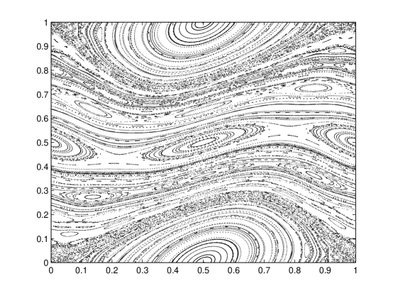
Figure 1. Plot of trajectories of the standard map for $\varepsilon=\frac{3}{4}$.

The map $f_{\varepsilon}$ can be recovered by its generating function $h:\mathbb{T}^{2}\rightarrow\mathbb{R}$ in the sense that, if $f_{\varepsilon}(x,y)=(X,Y)$, then $YdX-ydx=dh(x,X)$. Moreover, we have its action $\mathcal{A}$ which, for a sequence of points $\{x_{N},\dots,x_{M}\}$, is

(1) $$\mathcal{A}(x_{N},\dots,x_{M})=\sum_{k=N}^{M-1}h(x_{k},x_{k+1}),$$

such that trajectories of $f_{\varepsilon}$ “minimize” the action for fixed endpoints $\{x_{N},x_{M}\}$, in an analogous way to classical Lagrangian mechanics (see [Gol01, §2.5]).

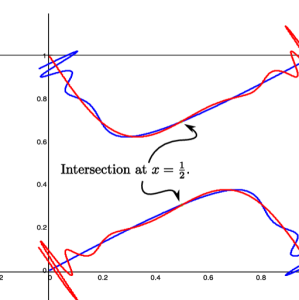
Figure 2. Intersection of the stable and unstable manifolds at $x=\frac{1}{2}$.

It follows from a simple symmetry argument that for all $\varepsilon\neq 0$, the stable and unstable manifolds of the hyperbolic fixed point intersect at $x=\frac{1}{2}$ (see Figure 2). Denote by $(\frac{1}{2},y_{\varepsilon})$ such a homoclinic point. It is rather easy to approximate this point numerically as one needs only to follow an approximation of either the stable or unstable manifold until it crosses $x=\frac{1}{2}$. Moreover, we can see from Figure 2 that between the point $(\frac{1}{2},y_{\varepsilon})$ and its image $f_{\varepsilon}(\frac{1}{2},y_{\varepsilon})=(\frac{1}{2}+y_{\varepsilon},y_{\varepsilon})$ there is homoclinic point which we denote as $(u,v)$. It is also relatively easy approximating numerically this point based on having a good approximation of the stable and unstable manifolds and the point $(\frac{1}{2},y_{\varepsilon})$. Using these points, one can proceed in two different ways in order to get index pairs for and isolated invariant set which belong to the homoclinic tangle of the fixed point.

The first way is to find the intersection of the stable and unstable manifolds at $x=\frac{1}{2}$ at high accuracy, and iterate this point enough times forward and backwards to get close enough to the fixed point. Considering all of these iterates and the fixed point as our invariant set, we may grow an isolating neighborhood and index pairs associated to them using Algorithm 3. This is perhaps the quickest way to get an index pair, as we already know where the isolated invariant set is. The downside is that in order for this approach to be successful, we need to compute the first homoclinic intersection with very high accuracy, as the homoclinic connection may be lengthy, and after enough iterations the error may become large enough to not give us a good approximation of the invariant set.

The second approach is to compute the connections using shortest path algorithms as in Algorithn 2. This approach requires less precision in the computation of the homoclinic intersection, but is slower than the first approach. However, it is faster than a blind shortest-path search because it takes in consideration the dynamics of $f_{\varepsilon}$: recalling the action (1) of $f_{\varepsilon}$, we have $\mathcal{A}(x_{1},x_{2})=h(x_{1},x_{2})$ and so we can compute the averaged action $\tilde{\mathcal{A}}:\mathcal{G}\times\mathcal{G}\rightarrow\mathbb{R}$ from box $\mathcal{B}_{i}$ to $\mathcal{B}_{j}$ as the average of $\mathcal{A}(x,y)$ with $x\in|\mathcal{B}_{i}|$ and $y\in|\mathcal{B}_{j}|$. Thus we can re-weigh the graph representing the map on boxes, from having every edge of weight 1, to having the edge going from $\mathcal{B}_{i}$ to $\mathcal{B}_{j}$ weight $K+\tilde{\mathcal{A}}(\mathcal{B}_{i},\mathcal{B}_{j})$, where $K$ is any positive number satisfying

$$K>K^{*}\equiv\max_{(x_{1},x_{2})\in\mathbb{T}^{2}}\left|\mathcal{A}(x_{1},x_{2})\right|,$$

uniform for all $\mathcal{B}_{i}$. Different choices of $K$ do not necessarily give the same shortest (or cheapest) path: higher $K$ gives more weight to the number of edges in the path (which one might use when working at a low depth), while lower $K$ gives more weight to the action (which one might use at a high depth). Thus, searching for shortest paths in the graph with the new weights, we have a better chance to compute the right connection at the first try, as the connections which are computed contain, on average, the least action from the beginning box to the end box.

This second method turns out to be a better fit in our setting, as numerically iterating the point $(\frac{1}{2},y_{\varepsilon})$ introduces error which is multiplied upon each iteration. Thus, the error grows exponentially fast until the iterates reach a small neighborhood of the fixed point, and this error is further exacerbated by the fact that we will mostly treat $\varepsilon$ as an interval. The second method still requires some precision, but it is modest enough that we can efficiently obtain it using the parameterization method [CFdlL05]. Algorithm 4 summarizes our construction of index pairs which contain the homoclinic tangle of the hyperbolic fixed point.

As $\varepsilon$ decreases, both the area of the Birkhoff zone of instability and the angle of intersection of stable and unstable manifolds of the hyperbolic fixed point $(\frac{1}{2},y_{\varepsilon})$ decrease exponentially fast with $\varepsilon$ [Gel99]. Thus since the intersection of the invariant manifolds is barely transversal, the index pairs associated to the homoclinic orbits have to stretch out considerably across the unstable manifolds in order to achieve isolation (see Figure 4). This in turn implies that Algorithm 3 takes more iterations to cover the invariant set. Moreover, the size of the boxes is necessarily exponentially small with $\varepsilon$, and so the number of boxes needed to create the index pairs increases rapidly. The bottom line is that the complete automation of the procedure prevents us of having to create the index pairs by hand, which for low $\varepsilon$ must be an extremely difficult task.

KAM theory asserts that for $|\varepsilon|$ small enough (roughly $|\varepsilon|<.971$ [Jun91]), there is a positive measure set of homotopically non-trivial invariant circles on which the dynamics of $f_{\varepsilon}$ is conjugate to irrational rotations. In this case the invariant circles folliate the cylinder and serve as obstructions to orbits from wandering all over the cylinder, i.e., each orbit is confined to an area bounded by KAM circles. In this case, the topological entropy of $f_{\varepsilon}$ is concentrated in the Birkhoff zone of instability associated to the homoclinic tangle of the hyperbolic fixed point. Once $\varepsilon>\varepsilon^{*}\approx.971$ there remain no homotopically non-trivial KAM circles to bound the $y$ coordinate of the orbit of a point and one has then hope to find connecting orbits between different hyperbolic periodic orbits.

We apply our methods to obtain three types of results:

• For all $f_{\varepsilon}$ with $\varepsilon\in[.7,2]$, we give a positive lower bound for its topological entropy. This is done by treating $\varepsilon$ as an interval. An advantage of having the procedure automated is that one can easily study a parameter-depending system at different values of the parameter. Treating the parameter as an interval allows us to detect behavior which is common to all values of the parameter in the interval. This is done in section 4.1.

• Not treating $\varepsilon$ as an interval allows our method to go further and obtains positive bounds for the much lower value of $\varepsilon=\frac{1}{2}$. This is done in section 4.2.

• Our examples in section 4.3 combine the new methods of this paper with the spirit of [DFT08] of connecting periodic orbits to find better entropy bounds, which will illustrate for the case $\varepsilon=2$.

We remark that in [MJ09, §4.1] an alternate approach for the creation of index pairs for the standard map is given. It is done through set-oriented methods which are based on following the discretized dynamics along the discretized stable and unstable manifolds. We do not know how this approach would perform when treating $\varepsilon$ as an interval, although we suspect it would perform equally well. Our bottom-up approach for constructing index pairs requires the computation of fewer box images, but in general we may make use of slightly more a-priori information such as the knowledge of where hyperbolic invariant sets are. The algorithms in [MJ09] (and indeed those of [DFT08, §3.1]) require less a-priori knowledge of hyperbolic, invariant sets, but require a greater number of box-image computations (see [MJ09] for more details).

We should point out that the bounds we provide in the following sections are close to some of the non-rigorous bounds given in [YT09]. To our knowledge there are no other bounds in the literature for the topological entropy of the standard map for small values of $\varepsilon$. It is expected that the entropy is exponentially small as $\varepsilon\rightarrow 0$ [Gel99], while it is known that the entropy grows at least logarithmically in $\varepsilon$ as $\epsilon\rightarrow\infty$ [Kni96]. But for small values of $\varepsilon$, we have not been able to find computational bounds besides the ones already cited.

4.1. Parameter exploration

As remarked earlier, when $\varepsilon<\varepsilon^{*}$ there exist invariant KAM circles which prevent the connections between many periodic orbits. This forces us to concentrate on the homoclinic tangle of the hyperbolic fixed point. The results from this section are obtained using Algorithm 4 and summarized in Theorem 4.1.

Algorithm 4 Creating index pairs for $f_{\varepsilon}$ using the homoclinic orbits of the fixed point

  Input: $\bar{\varepsilon}=[\varepsilon^{-},\varepsilon^{+}]$, $f_{\bar{\varepsilon}}$

  Let $y_{\bar{\varepsilon}}=y_{\frac{\varepsilon^{-}+\varepsilon^{+}}{2}}$ and compute $\left(\frac{1}{2},y_{\bar{\varepsilon}}\right)$ using [CFdlL05].

  $H=\left\{\left(\frac{1}{2},y_{\bar{\varepsilon}}\right),\left(\frac{1}{2},1-y_{\bar{\varepsilon}}\right),(u,v),(1-u,1-v),(0,0)\right\}$

  $X=\bigcup_{p\neq q\in H}(p,q)$

  Find connections using Algorithm 2 and the weighted graph using the averaged action $\tilde{\mathcal{A}}$.

  Grow the index pairs using Algorithm 3.

By performing the computations using $\varepsilon$ as an interval, we are proving behavior which is common for all $f_{\varepsilon}$ within such interval. In such case then our guess for the homoclinic intersection $(\frac{1}{2},y_{\varepsilon})$ is done only for one point in the interval (the midpoint). In general it is easier to isolate an invariant set for smaller parameter intervals, since the wider the interval, the more general the isolation must be. In our setting, it is much easier to isolate homoclinic connections for $\varepsilon>\varepsilon^{*}$ than it is for $\varepsilon<\varepsilon^{*}$. To reflect this, using a crude approximation of $\varepsilon^{*}\approx 1.0$ for ease of bookkeeping, we use intervals of size 0.005 for $\varepsilon\geq 1.0$, but we shrink our interval size to 0.001 for $\varepsilon<1.0$.

As $\varepsilon$ decreases, the size of the boxes we use decreases, and the length of the homoclinic excursion increases, leading to another increase in the number of boxes needed and a longer running time of Algorithm 3. At some point, it becomes computationaly unrealistic to continue; we stopped somewhat before this point, when the interval computations took roughly 40 hours for $\bar{\varepsilon}=[0.700,0.701]$. See section 4.4 for further discussion of the implementation and efficiency.

Theorem 4.1.

The topological entropy of the standard map $f_{\varepsilon}$ for $\varepsilon\in[.7,2]$ is bounded from below by the step function given in Figure 3. In particular, we have $h(f_{\varepsilon})>0.2$ for all $\varepsilon\in[.7,2]$. The precise individual values for each subinterval are given in Appendix A.

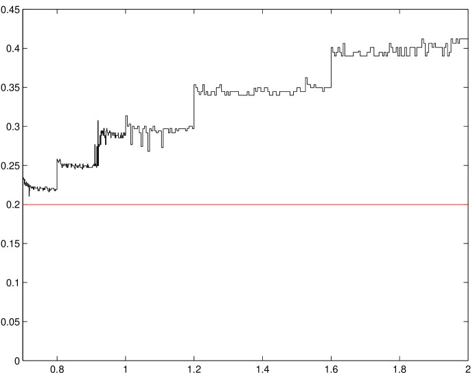
Figure 3. Lower bounds of $h(f_{\varepsilon})$ as a function of ${\varepsilon}$ in the interval $[.7,2]$. Note that all bounds in this interval exceed $0.2$.

Proof.

For each of the $\varepsilon$-intervals $\bar{\varepsilon}=[\varepsilon^{-},\varepsilon^{+}]$ on the table found in Appendix A, we get an index pair for an isolated invariant set of $f_{\bar{\varepsilon}}$ using Algorithm 4. Using then Algorithm 5, 6, 7, and 8 and Theorem 3.6 from [DFT08], which is essentially amounts to a finite number of checks using Corollary 2.13, we prove a semi-conjugacy to a subshift of finite type, from which we get a bound on the entropy by bounding the spectral radius of the associated matrix. ∎

There are three aparent scales on which our lower bounds for $h(f_{\varepsilon})$ change with respect to $\varepsilon$: global, semi-local, and local. Clearly there is an evident global increase of the entropy bounds as $\varepsilon$ increases, as is to expected. On a semi-local level, there are a few intervals (roughly $[1.6,2],[1.2,1.6]$, $[.92,1.2]$, $[.8,.92]$, $[.75,.8]$) on which the bounds for $h(f_{\varepsilon})$ seem to hover around a fixed value per interval. This is due to using the same depth on such intervals. As $\varepsilon$ decreases, we need to increase the depth. Locally, the apparent irregularity of the function of lower bounds is due to the nature of our automated approach: the accuracy of the guess $\left(\frac{1}{2},y_{\bar{\varepsilon}}\right)$ varies per interval, as does the computation of the averaged action, et cetera.

4.2. Positive bound of $h(f_{\varepsilon})$ for lowest $\varepsilon$.

In this section we show an example of an index pair for the standard map for $\varepsilon=\frac{1}{2}$. This value was picked because it is small enough that we can illustrate the strengths of our algorithms in tight places while keeping the computation times reasonable. Using Algorithm 4 with $\varepsilon=\frac{1}{2}$ we get an index pair shown in Figure 4 (although it is barely visible).

Theorem 4.2.

The topological entropy for the standard map $f_{\varepsilon}$ when $\varepsilon=\frac{1}{2}$ is bounded below by $0.1732515918346$.

The proof is the same as in Theorem 4.1. The tree from which the index pair obtained for Theorem 4.2 was obtained contains 568,754 boxes. Among those, 281,530 are in the index pair. Roughly a quarter of the boxes in the index pair form the exit set (64,518). This index pair $(P_{1},P_{0})$ gives us an induced map which acts on $H_{1}(P_{1},P_{0};\mathbb{Z})=\mathbb{Z}^{1801}$ but is reduced to a SFT in 73 symbols.

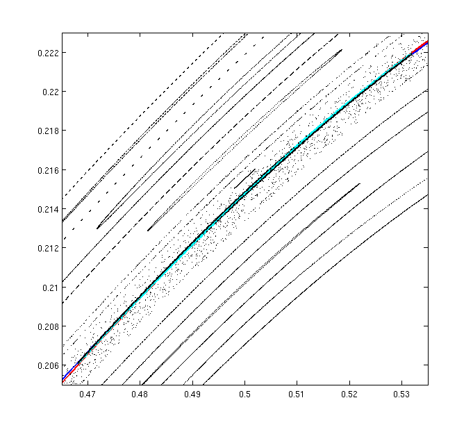
Figure 4. On top, a plot of the trajectories of the standard map for $\varepsilon=\frac{1}{2}$ along with the stable and unstable manifolds of the hyperbolic fixed point which seem to overlap. On the bottom, a close-up of a component of the index pair yielding Theorem 4.2 which contains the homoclinic point at $x=\frac{1}{2}$ along with trajectories, some of which are part of KAM circles squeezing the component. It overlays the stable and unstable manifolds, whose angle of intersection is very small, causing the index pair to be very sheared.

Figure 4 shows, on top, the plot of some trajectories for the standard map at $\varepsilon=\frac{1}{2}$, of the stable and unstable manifolds, and an index pair for the homoclinic orbits. On the bottom is a close-up to a component of the index pair squeezed by KAM tori and a barely transversal intersection of the stable and unstable manifolds. The boxes making up this index pair are of sides of size $2^{-15}$. The strength of our “growing-out” approach is that the creation of such index pairs in tight places is achievable and can be automated.

4.3. Higher periods

When $\varepsilon>\varepsilon^{*}$ all homotopically non-trivial KAM circles are vanished, thus it is possible to connect different periodic orbits. The appendix of [Gre79] contains an algorithm for finding periodic orbits for the standard map. We implement this method to find the periodic orbits which we use to grow index pairs.

Algorithm 5 Creating index pairs using the homoclinic orbits of the fixed point and periodic orbits

  Input: $\bar{\varepsilon}=[\varepsilon^{-},\varepsilon^{+}]$, $f_{\bar{\varepsilon}}$, $P\in\mathbb{N}$

  Let $y_{\bar{\varepsilon}}=y_{\frac{\varepsilon^{-}+\varepsilon^{+}}{2}}$ and compute $\left(\frac{1}{2},y_{\bar{\varepsilon}}\right)$ using [CFdlL05].

  $H_{1}=\left\{(0,0),\left(\frac{1}{2},y_{\bar{\varepsilon}}\right),\left(\frac{1}{2},1-y_{\bar{\varepsilon}}\right),(u,v),(1-u,1-v)\right\}$

  $H_{2}=$ hyperbolic periodic orbits of $f_{\bar{\varepsilon}}$ up to period $P$ (computed using the appendix in [Gre79])

  $X=\bigcup_{p\neq q\in(H_{1}\cup H_{2})}(p,q)$

  Find connections using Algorithm 2 and the weighted graph using averaged action $\tilde{\mathcal{A}}$.

  Grow the index pairs using Algorithm 3.

Algorithm 5 is essentially the main strategy employed in [DFT08]. In that paper, good index pairs were found by finding pairwise connections between periodic orbits. Such an approach can be slightly generalized by looking for pairwise connections between hyperbolic, invariant sets, which is what Algorithm 5 does.

We apply the algorithm to $\varepsilon=2.0$, with maximum period $P=2$. Figure 5 shows the index pair for this computation. We remark that besides finding pairwise connections between hyperbolic periodic orbits, we find connections between periodic orbits and the homoclinic orbit $(\frac{1}{2},y_{\varepsilon})$ and $(u,v)$ mentioned in section 4.1. This allows us to find richer dynamics and to achieve higher entropy bounds. The result from this index pair is summarized in the following theorem.

Theorem 4.3.

The topological entropy for the standard map $f_{\varepsilon}$ for $\varepsilon=2$ is bounded below by $0.44722970117798$.

The proof is again similar to Theorem 4.1. The index pair $(P_{1},P_{0})$ has a total of 8600 boxes, and gives us an induced map which acts on $H_{1}(P_{1},P_{0};\mathbb{Z})=\mathbb{Z}^{105}$ which is reduced to a SFT in 59 symbols.

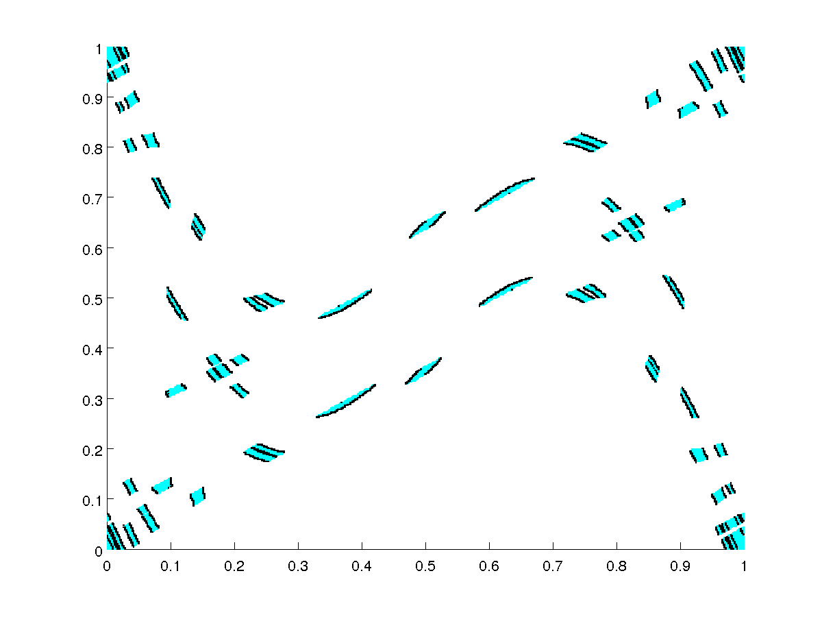
Figure 5. Index pair obtained through Algorithm 5 for $\varepsilon=2$ and $P=2$ at depth $9$.

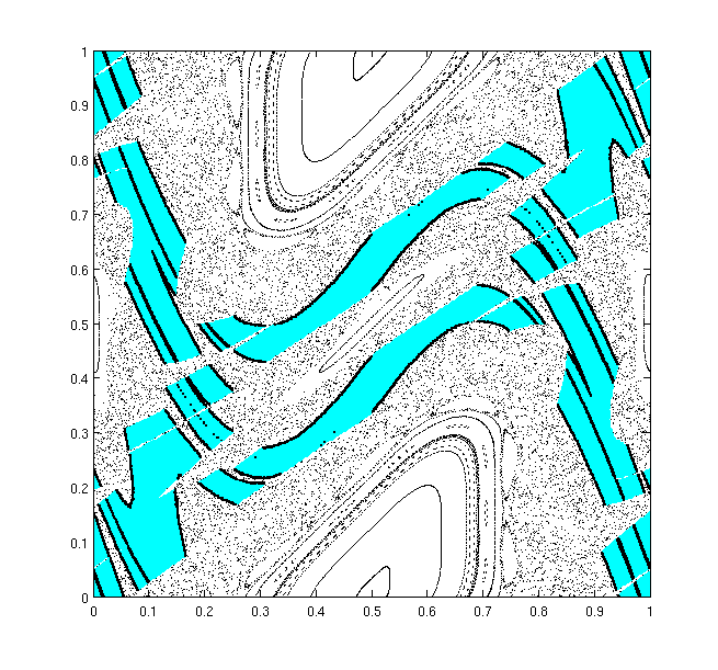
Figure 6. Index pair obtained by adding periodic orbits of period 3 and 4 to the example in Figure 5

This result shows that our bounds in Theorem 4.1 are probably suboptimal, since our interval bound for $[1.995,2.000]$ is lower than in Theorem 4.3. It is not surprising that by adding connections to another hyperbolic periodic orbit we may find a higher entropy bound.

Algorithm 5 can be quite effective when $P$ is small, but as $P$ grows, there is large increase (quadratic at the very least, often exponential) in the number of connections to compute, especially since the number of period-$P$ orbits grows rapidly with $P$ for chaotic maps. Moreover, the number of long connections increases, which as discussed in section 3.2 makes Algorithm 2 work even harder. As suggested in that section, we instead turn to computing periodic orbits of higher period rather than computing connections explicitly.

For our last example, we apply this approach on top of the previous example from Theorem 4.3 to produce a very strong index pair. That is, we run Algorithm 5 with $P=2$ and then simply add all hyperbolic orbits of period 3 and 4 (there are four of each) without adding any further connections. The resulting index pair, shown in Figure 6, clearly benefits from these “natural” connections.

Theorem 4.4.

The topological entropy for the standard map $f_{\varepsilon}$ for $\varepsilon=2$ is bounded below by $0.54518888942276$.

The index pair $(P_{1},P_{0})$ for Theorem 4.4 has a total of 64,185 boxes, with 5,839 in the exit set. The induced map acts on $H_{1}(P_{1},P_{0};\mathbb{Z})=\mathbb{Z}^{138}$ and reduces to a SFT on only 41 symbols.

4.4. Notes on efficiency and implementation

The computations in this paper were performed in MATLAB on machines with between 1 and 2 gigabytes (GB) of memory and with clock speeds between 1.5 and 2.5 gigahertz. Runtimes ranged from 3 or 4 minutes for $\bar{\varepsilon}=[1.995,2]$ and $\varepsilon=2.0$, to almost 2 days for $\bar{\varepsilon}=[0.700,0.701]$ and roughly 5 days for $\varepsilon=0.5$. As discussed in section 4.1 and the beginning of section 4, there was a roughly inverse exponential relationship between $\varepsilon$ and the runtime for the intermediate values.

The two most time-consuming subroutines for our computations were Algorithms 2 and 3, which of course is one reason for our focus on them in this work. As $\varepsilon$ decreased, however, Algorithm 3 dominated the runtime, particularly in the bookkeeping step (maintaining the correct box numbers, as discussed in section 3.1) and the insertion step, when new boxes are inserted into the tree. While the insertions cannot be avoided, this does suggest that a better tree implementation could enhance performance greatly.

To conclude, we would like to reiterate how difficult it would be to reproduce our results for low $\varepsilon$, namely Theorem 4.2 and the lower intervals of Theorem 4.1, using index pair algorithms from [DFT08]. As mentioned in section 3.3, our algorithms are considerably more memory efficient in certain situations, which we now explore concretely. Consider the index pair we obtained in Theorem 4.2 when $\varepsilon=0.5$; there were 568754 boxes in the index pair, at depth 15, and the adjacency and transition matrices took up about 0.1GB of memory using our approach. Using the [DFT08] approach, one would need to compute the map on all boxes at depth 15. Using a conservative estimate of 190 bytes per box to store the image and adjacency information (the average for our index pair was 194.38 bytes), this would require 204GB, which is beyond reasonable at the time of this writing. More to the point, our bottom-up approach is clearly orders of magnitude more efficient in terms of memory. When one considers the graph computations that would need to be carried out on the resulting $2^{30}$-node graph (the transition matrix), it becomes even clearer that our computations would have been impractical using the top-down approach of [DFT08].

Appendix A Precise bounds for $h(f_{\varepsilon})$

Below we list the actual values for the lower bounds in Theorem 4.1 the last column indicates the number of symbols for each SFT whose entropy bounds that of $f_{\varepsilon}$ for $\varepsilon$ in each interval.

$\varepsilon$ interval	$h(f_{\varepsilon})\geq$	sym
[0.700, 0.701]	0.232286	51
[0.701, 0.702]	0.234189	51
[0.702, 0.703]	0.232286	51
[0.703, 0.704]	0.232286	51
[0.704, 0.705]	0.225504	53
[0.705, 0.706]	0.232286	51
[0.706, 0.707]	0.227178	51
[0.707, 0.708]	0.227178	51
[0.708, 0.709]	0.223988	53
[0.709, 0.710]	0.227178	53
[0.710, 0.711]	0.228742	53
[0.711, 0.712]	0.223988	53
[0.712, 0.713]	0.223988	53
[0.713, 0.714]	0.223988	53
[0.714, 0.715]	0.227178	53
[0.715, 0.716]	0.222542	53
[0.716, 0.717]	0.222365	53
[0.717, 0.718]	0.225679	53
[0.718, 0.719]	0.210614	39
[0.719, 0.720]	0.217650	55
[0.720, 0.721]	0.223988	53
[0.721, 0.722]	0.223988	53
[0.722, 0.723]	0.223988	53
[0.723, 0.724]	0.222542	53
[0.724, 0.725]	0.222542	53
[0.725, 0.726]	0.220813	55
[0.726, 0.727]	0.222542	53
[0.727, 0.728]	0.222542	53
[0.728, 0.729]	0.222542	55
[0.729, 0.730]	0.220813	55
[0.730, 0.731]	0.222365	55
[0.731, 0.732]	0.219153	55
[0.732, 0.733]	0.219153	55
[0.733, 0.734]	0.222542	55
[0.734, 0.735]	0.222542	55
[0.735, 0.736]	0.222542	55
[0.736, 0.737]	0.220813	55
[0.737, 0.738]	0.220813	55
[0.738, 0.739]	0.220813	55
[0.739, 0.740]	0.220813	55
[0.740, 0.741]	0.220813	55
[0.741, 0.742]	0.220813	55
[0.742, 0.743]	0.222542	55
[0.743, 0.744]	0.220813	55
[0.744, 0.745]	0.217650	55
[0.745, 0.746]	0.219153	55
[0.746, 0.747]	0.217650	55
[0.747, 0.748]	0.217650	55
[0.748, 0.749]	0.217650	55
[0.749, 0.750]	0.220813	55
[0.750, 0.751]	0.222542	55
[0.751, 0.752]	0.220813	55
[0.752, 0.753]	0.220813	55
[0.753, 0.754]	0.220813	55
[0.754, 0.755]	0.220813	55
[0.755, 0.756]	0.220813	55

$\varepsilon$ interval	$h(f_{\varepsilon})\geq$	sym
[0.756, 0.757]	0.220813	55
[0.757, 0.758]	0.220813	55
[0.758, 0.759]	0.219153	55
[0.759, 0.760]	0.217650	55
[0.760, 0.761]	0.220813	55
[0.761, 0.762]	0.219153	55
[0.762, 0.763]	0.220813	55
[0.763, 0.764]	0.219153	55
[0.764, 0.765]	0.219153	55
[0.765, 0.766]	0.222542	55
[0.766, 0.767]	0.222542	55
[0.767, 0.768]	0.222542	55
[0.768, 0.769]	0.222542	55
[0.769, 0.770]	0.222542	55
[0.770, 0.771]	0.220813	55
[0.771, 0.772]	0.220813	55
[0.772, 0.773]	0.220813	55
[0.773, 0.774]	0.217650	55
[0.774, 0.775]	0.217650	55
[0.775, 0.776]	0.217650	55
[0.776, 0.777]	0.216045	55
[0.777, 0.778]	0.220813	55
[0.778, 0.779]	0.219153	55
[0.779, 0.780]	0.217650	55
[0.780, 0.781]	0.219153	55
[0.781, 0.782]	0.219153	55
[0.782, 0.783]	0.219153	55
[0.783, 0.784]	0.219153	55
[0.784, 0.785]	0.220813	55
[0.785, 0.786]	0.220813	55
[0.786, 0.787]	0.220813	55
[0.787, 0.788]	0.220813	55
[0.788, 0.789]	0.220813	55
[0.789, 0.790]	0.220813	55
[0.790, 0.791]	0.220813	55
[0.791, 0.792]	0.219153	55
[0.792, 0.793]	0.217650	55
[0.793, 0.794]	0.217650	55
[0.794, 0.795]	0.219153	55
[0.795, 0.796]	0.217650	55
[0.796, 0.797]	0.219153	55
[0.797, 0.798]	0.219153	55
[0.798, 0.799]	0.219153	55
[0.799, 0.800]	0.219153	55
[0.800, 0.801]	0.257972	43
[0.801, 0.802]	0.255740	45
[0.802, 0.803]	0.255740	43
[0.803, 0.804]	0.255740	43
[0.804, 0.805]	0.253746	45
[0.805, 0.806]	0.255740	45
[0.806, 0.807]	0.255740	45
[0.807, 0.808]	0.255740	45
[0.808, 0.809]	0.257972	43
[0.809, 0.810]	0.255740	45
[0.810, 0.811]	0.251858	45
[0.811, 0.812]	0.251858	45

$\varepsilon$ interval	$h(f_{\varepsilon})\geq$	sym
[0.812, 0.813]	0.251858	45
[0.813, 0.814]	0.249549	45
[0.814, 0.815]	0.247344	47
[0.815, 0.816]	0.247344	47
[0.816, 0.817]	0.251858	47
[0.817, 0.818]	0.249549	45
[0.818, 0.819]	0.249549	47
[0.819, 0.820]	0.249549	47
[0.820, 0.821]	0.251858	45
[0.821, 0.822]	0.251858	47
[0.822, 0.823]	0.251858	45
[0.823, 0.824]	0.251858	47
[0.824, 0.825]	0.249549	47
[0.825, 0.826]	0.249549	47
[0.826, 0.827]	0.249549	47
[0.827, 0.828]	0.251858	47
[0.828, 0.829]	0.247344	47
[0.829, 0.830]	0.251858	45
[0.830, 0.831]	0.247344	47
[0.831, 0.832]	0.247344	47
[0.832, 0.833]	0.249549	47
[0.833, 0.834]	0.251858	47
[0.834, 0.835]	0.251858	47
[0.835, 0.836]	0.251858	47
[0.836, 0.837]	0.251858	47
[0.837, 0.838]	0.251858	47
[0.838, 0.839]	0.251858	47
[0.839, 0.840]	0.251858	47
[0.840, 0.841]	0.251858	47
[0.841, 0.842]	0.247610	47
[0.842, 0.843]	0.251858	47
[0.843, 0.844]	0.251858	47
[0.844, 0.845]	0.249549	47
[0.845, 0.846]	0.249549	47
[0.846, 0.847]	0.249549	47
[0.847, 0.848]	0.249549	47
[0.848, 0.849]	0.249549	47
[0.849, 0.850]	0.249549	47
[0.850, 0.851]	0.247344	47
[0.851, 0.852]	0.247344	47
[0.852, 0.853]	0.245376	47
[0.853, 0.854]	0.251858	47
[0.854, 0.855]	0.251858	47
[0.855, 0.856]	0.249549	47
[0.856, 0.857]	0.249549	47
[0.857, 0.858]	0.249549	47
[0.858, 0.859]	0.247344	47
[0.859, 0.860]	0.247344	47
[0.860, 0.861]	0.249549	47
[0.861, 0.862]	0.247344	47
[0.862, 0.863]	0.249549	47
[0.863, 0.864]	0.249549	47
[0.864, 0.865]	0.249549	47
[0.865, 0.866]	0.249549	47
[0.866, 0.867]	0.251858	47
[0.867, 0.868]	0.247344	47

$\varepsilon$ interval	$h(f_{\varepsilon})\geq$	sym
[0.868, 0.869]	0.247344	47
[0.869, 0.870]	0.247344	47
[0.870, 0.871]	0.247344	47
[0.871, 0.872]	0.247344	47
[0.872, 0.873]	0.247344	47
[0.873, 0.874]	0.245376	47
[0.874, 0.875]	0.245376	47
[0.875, 0.876]	0.251858	47
[0.876, 0.877]	0.249549	47
[0.877, 0.878]	0.247344	47
[0.878, 0.879]	0.249549	47
[0.879, 0.880]	0.249549	47
[0.880, 0.881]	0.249549	47
[0.881, 0.882]	0.249549	47
[0.882, 0.883]	0.249549	47
[0.883, 0.884]	0.249549	47
[0.884, 0.885]	0.249549	47
[0.885, 0.886]	0.249549	47
[0.886, 0.887]	0.247344	47
[0.887, 0.888]	0.247344	47
[0.888, 0.889]	0.249549	47
[0.889, 0.890]	0.251858	47
[0.890, 0.891]	0.247344	47
[0.891, 0.892]	0.249549	47
[0.892, 0.893]	0.247344	47
[0.893, 0.894]	0.247344	47
[0.894, 0.895]	0.247344	47
[0.895, 0.896]	0.247344	47
[0.896, 0.897]	0.247344	47
[0.897, 0.898]	0.247344	47
[0.898, 0.899]	0.247344	47
[0.899, 0.900]	0.247344	47
[0.900, 0.901]	0.247344	47
[0.901, 0.902]	0.247344	47
[0.902, 0.903]	0.247344	47
[0.903, 0.904]	0.249549	47
[0.904, 0.905]	0.249549	47
[0.905, 0.906]	0.249549	47
[0.906, 0.907]	0.249549	47
[0.907, 0.908]	0.251858	47
[0.908, 0.909]	0.249549	47
[0.909, 0.910]	0.249549	47
[0.910, 0.911]	0.276723	27
[0.911, 0.912]	0.249549	47
[0.912, 0.913]	0.251858	47
[0.913, 0.914]	0.249549	47
[0.914, 0.915]	0.249549	47
[0.915, 0.916]	0.247344	47
[0.916, 0.917]	0.274243	27
[0.917, 0.918]	0.249549	47
[0.918, 0.919]	0.257110	25
[0.919, 0.920]	0.307453	35
[0.920, 0.921]	0.249549	47
[0.921, 0.922]	0.276723	27
[0.922, 0.923]	0.276723	27
[0.923, 0.924]	0.274243	27

$\varepsilon$ interval	$h(f_{\varepsilon})\geq$	sym
[0.924, 0.925]	0.276723	27
[0.925, 0.926]	0.288442	37
[0.926, 0.927]	0.276723	27
[0.927, 0.928]	0.276723	27
[0.928, 0.929]	0.294293	37
[0.929, 0.930]	0.288442	37
[0.930, 0.931]	0.294293	37
[0.931, 0.932]	0.291280	37
[0.932, 0.933]	0.291280	37
[0.933, 0.934]	0.294293	37
[0.934, 0.935]	0.288442	37
[0.935, 0.936]	0.288442	39
[0.936, 0.937]	0.297475	37
[0.937, 0.938]	0.297475	37
[0.938, 0.939]	0.288442	39
[0.939, 0.940]	0.285349	39
[0.940, 0.941]	0.288442	39
[0.941, 0.942]	0.276723	27
[0.942, 0.943]	0.276723	27
[0.943, 0.944]	0.294293	37
[0.944, 0.945]	0.294293	37
[0.945, 0.946]	0.297475	37
[0.946, 0.947]	0.294293	37
[0.947, 0.948]	0.291706	39
[0.948, 0.949]	0.291706	39
[0.949, 0.950]	0.288442	39
[0.950, 0.951]	0.291706	39
[0.951, 0.952]	0.291706	39
[0.952, 0.953]	0.291706	39
[0.953, 0.954]	0.294293	37
[0.954, 0.955]	0.294293	37
[0.955, 0.956]	0.291706	39
[0.956, 0.957]	0.291706	37
[0.957, 0.958]	0.285349	39
[0.958, 0.959]	0.291706	39
[0.959, 0.960]	0.291706	39
[0.960, 0.961]	0.291706	39
[0.961, 0.962]	0.291706	39
[0.962, 0.963]	0.288442	39
[0.963, 0.964]	0.288442	39
[0.964, 0.965]	0.291706	39
[0.965, 0.966]	0.291706	39
[0.966, 0.967]	0.291706	39
[0.967, 0.968]	0.288442	39
[0.968, 0.969]	0.288442	39
[0.969, 0.970]	0.285349	39
[0.970, 0.971]	0.291706	39
[0.971, 0.972]	0.285349	39
[0.972, 0.973]	0.288442	39
[0.973, 0.974]	0.288442	39
[0.974, 0.975]	0.288442	39
[0.975, 0.976]	0.288442	39
[0.976, 0.977]	0.288442	39
[0.977, 0.978]	0.288442	39
[0.978, 0.979]	0.291706	39
[0.979, 0.980]	0.285349	39

$\varepsilon$ interval	$h(f_{\varepsilon})\geq$	sym
[0.980, 0.981]	0.285349	39
[0.981, 0.982]	0.285349	39
[0.982, 0.983]	0.285349	39
[0.983, 0.984]	0.285349	39
[0.984, 0.985]	0.285349	39
[0.985, 0.986]	0.288442	39
[0.986, 0.987]	0.285349	39
[0.987, 0.988]	0.291706	39
[0.988, 0.989]	0.285349	39
[0.989, 0.990]	0.285349	39
[0.990, 0.991]	0.285349	39
[0.991, 0.992]	0.288442	39
[0.992, 0.993]	0.285349	39
[0.993, 0.994]	0.291706	39
[0.994, 0.995]	0.291706	39
[0.995, 0.996]	0.291706	39
[0.996, 0.997]	0.288442	39
[0.997, 0.998]	0.291706	39
[0.998, 0.999]	0.288442	39
[0.999, 1.000]	0.288442	39
[1.000, 1.005]	0.313677	35
[1.005, 1.010]	0.300202	35
[1.010, 1.015]	0.303084	35
[1.015, 1.020]	0.276723	27
[1.020, 1.025]	0.300202	35
[1.025, 1.030]	0.297053	37
[1.030, 1.035]	0.297053	37
[1.035, 1.040]	0.300202	35
[1.040, 1.045]	0.291706	37
[1.045, 1.050]	0.274243	36
[1.050, 1.055]	0.297053	39
[1.055, 1.060]	0.300202	37
[1.060, 1.065]	0.291706	37
[1.065, 1.070]	0.267938	39
[1.070, 1.075]	0.297053	36
[1.075, 1.080]	0.294293	37
[1.080, 1.085]	0.300202	37
[1.085, 1.090]	0.294293	37
[1.090, 1.095]	0.291706	37
[1.095, 1.100]	0.294293	37
[1.100, 1.105]	0.294293	37
[1.105, 1.110]	0.272833	39
[1.110, 1.115]	0.297053	37
[1.115, 1.120]	0.297053	37
[1.120, 1.125]	0.297053	37
[1.125, 1.130]	0.291706	37
[1.130, 1.135]	0.297475	37
[1.135, 1.140]	0.291706	37
[1.140, 1.145]	0.291706	37
[1.145, 1.150]	0.297053	37
[1.150, 1.155]	0.294293	37
[1.155, 1.160]	0.297053	37
[1.160, 1.165]	0.297053	37
[1.165, 1.170]	0.297053	37
[1.170, 1.175]	0.297053	37
[1.175, 1.180]	0.294293	37

$\varepsilon$ interval	$h(f_{\varepsilon})\geq$	sym
[1.180, 1.185]	0.297475	37
[1.185, 1.190]	0.300202	37
[1.190, 1.195]	0.300202	37
[1.195, 1.200]	0.297053	37
[1.200, 1.205]	0.353423	31
[1.205, 1.210]	0.349617	29
[1.210, 1.215]	0.344595	29
[1.215, 1.220]	0.340662	31
[1.220, 1.225]	0.344595	29
[1.225, 1.230]	0.353423	29
[1.230, 1.235]	0.340662	31
[1.235, 1.240]	0.344595	29
[1.240, 1.245]	0.339892	31
[1.245, 1.250]	0.339892	29
[1.250, 1.255]	0.344595	31
[1.255, 1.260]	0.344595	31
[1.260, 1.265]	0.339892	31
[1.265, 1.270]	0.349617	31
[1.270, 1.275]	0.349617	31
[1.275, 1.280]	0.353423	31
[1.280, 1.285]	0.344595	31
[1.285, 1.290]	0.344595	31
[1.290, 1.295]	0.339892	31
[1.295, 1.300]	0.344595	31
[1.300, 1.305]	0.339892	31
[1.305, 1.310]	0.344595	31
[1.310, 1.315]	0.344595	31
[1.315, 1.320]	0.344595	31
[1.320, 1.325]	0.344595	31
[1.325, 1.330]	0.344595	31
[1.330, 1.335]	0.339892	29
[1.335, 1.340]	0.339892	31
[1.340, 1.345]	0.339892	31
[1.345, 1.350]	0.339892	31
[1.350, 1.355]	0.339892	31
[1.355, 1.360]	0.344595	31
[1.360, 1.365]	0.339892	31
[1.365, 1.370]	0.339892	31
[1.370, 1.375]	0.339892	31
[1.375, 1.380]	0.348848	31
[1.380, 1.385]	0.344595	31
[1.385, 1.390]	0.349617	31
[1.390, 1.395]	0.349617	31
[1.395, 1.400]	0.344595	31
[1.400, 1.405]	0.344595	31
[1.405, 1.410]	0.349617	31
[1.410, 1.415]	0.349617	31
[1.415, 1.420]	0.344595	31
[1.420, 1.425]	0.339892	31
[1.425, 1.430]	0.339892	31
[1.430, 1.435]	0.344595	31
[1.435, 1.440]	0.344595	31
[1.440, 1.445]	0.339892	29
[1.445, 1.450]	0.339892	31
[1.450, 1.455]	0.344595	31
[1.455, 1.460]	0.344595	31

$\varepsilon$ interval	$h(f_{\varepsilon})\geq$	sym
[1.460, 1.465]	0.344595	31
[1.465, 1.470]	0.344595	31
[1.470, 1.475]	0.344595	31
[1.475, 1.480]	0.344595	31
[1.480, 1.485]	0.339892	31
[1.485, 1.490]	0.339892	31
[1.490, 1.495]	0.344595	31
[1.495, 1.500]	0.344595	31
[1.500, 1.505]	0.349617	31
[1.505, 1.510]	0.349617	31
[1.510, 1.515]	0.344595	31
[1.515, 1.520]	0.344595	31
[1.520, 1.525]	0.344595	31
[1.525, 1.530]	0.362385	29
[1.530, 1.535]	0.353822	29
[1.535, 1.540]	0.353423	31
[1.540, 1.545]	0.349617	29
[1.545, 1.550]	0.349617	29
[1.550, 1.555]	0.353423	29
[1.555, 1.560]	0.349617	29
[1.560, 1.565]	0.349617	29
[1.565, 1.570]	0.349617	29
[1.570, 1.575]	0.349617	29
[1.575, 1.580]	0.344595	29
[1.580, 1.585]	0.349617	29
[1.585, 1.590]	0.349617	31
[1.590, 1.595]	0.349617	29
[1.595, 1.600]	0.349617	29
[1.600, 1.605]	0.401206	25
[1.605, 1.610]	0.394853	25
[1.610, 1.615]	0.390054	25
[1.615, 1.620]	0.394853	27
[1.620, 1.625]	0.401206	25
[1.625, 1.630]	0.394853	25
[1.630, 1.635]	0.390054	25
[1.635, 1.640]	0.406401	23
[1.640, 1.645]	0.390054	27
[1.645, 1.650]	0.390054	25
[1.650, 1.655]	0.390054	25
[1.655, 1.660]	0.390054	27
[1.660, 1.665]	0.390054	27
[1.665, 1.670]	0.394853	25
[1.670, 1.675]	0.394853	25
[1.675, 1.680]	0.394853	25
[1.680, 1.685]	0.396415	25
[1.685, 1.690]	0.390054	27
[1.690, 1.695]	0.390054	25
[1.695, 1.700]	0.390054	25
[1.700, 1.705]	0.390054	25
[1.705, 1.710]	0.394853	25
[1.710, 1.715]	0.394853	25
[1.715, 1.720]	0.401206	25
[1.720, 1.725]	0.401206	27
[1.725, 1.730]	0.390054	25
[1.730, 1.735]	0.390054	25
[1.735, 1.740]	0.390054	27

$\varepsilon$ interval	$h(f_{\varepsilon})\geq$	sym
[1.740, 1.745]	0.394853	25
[1.745, 1.750]	0.394853	25
[1.750, 1.755]	0.390054	25
[1.755, 1.760]	0.394853	25
[1.760, 1.765]	0.390054	27
[1.765, 1.770]	0.394853	25
[1.770, 1.775]	0.406401	25
[1.775, 1.780]	0.401206	25
[1.780, 1.785]	0.394853	25
[1.785, 1.790]	0.394853	25
[1.790, 1.795]	0.401206	25
[1.795, 1.800]	0.390054	25
[1.800, 1.805]	0.401206	25
[1.805, 1.810]	0.390054	25
[1.810, 1.815]	0.390054	27
[1.815, 1.820]	0.401206	25
[1.820, 1.825]	0.390054	25
[1.825, 1.830]	0.390054	25
[1.830, 1.835]	0.401206	27
[1.835, 1.840]	0.401206	25
[1.840, 1.845]	0.401206	25
[1.845, 1.850]	0.390054	27
[1.850, 1.855]	0.401206	25
[1.855, 1.860]	0.401206	25
[1.860, 1.865]	0.401206	27
[1.865, 1.870]	0.411995	25
[1.870, 1.875]	0.406401	25
[1.875, 1.880]	0.390054	25
[1.880, 1.885]	0.394853	25
[1.885, 1.890]	0.406401	25
[1.890, 1.895]	0.406401	25
[1.895, 1.900]	0.401206	25
[1.900, 1.905]	0.406401	25
[1.905, 1.910]	0.401206	25
[1.910, 1.915]	0.401206	25
[1.915, 1.920]	0.401206	25
[1.920, 1.925]	0.401206	25
[1.925, 1.930]	0.390054	25
[1.930, 1.935]	0.401206	25
[1.935, 1.940]	0.406401	25
[1.940, 1.945]	0.390054	25
[1.945, 1.950]	0.394853	25
[1.950, 1.955]	0.411995	25
[1.955, 1.960]	0.406401	25
[1.960, 1.965]	0.406401	25
[1.965, 1.970]	0.411995	25
[1.970, 1.975]	0.406401	23
[1.975, 1.980]	0.411995	23
[1.980, 1.985]	0.411995	25
[1.985, 1.990]	0.411995	23
[1.990, 1.995]	0.411995	25
[1.995, 2.000]	0.411995	25

References

- [BCG07] Balázs Bánhelyi, Tibor Csendes, and Barnabas M. Garay, Optimization and the Miranda approach in detecting horseshoe-type chaos by computer, Internat. J. Bifur. Chaos Appl. Sci. Engrg. 17 (2007), no. 3, 735–747. MR MR2324978 (2008d:37047)
- [BCGH08] Balázs Bánhelyi, Tibor Csendes, Barnabas M. Garay, and László Hatvani, A computer-assisted proof of -chaos in the forced damped pendulum equation, SIAM J. Appl. Dyn. Syst. 7 (2008), no. 3, 843–867. MR MR2443025 (2009g:37029)
- [CFdlL05] Xavier Cabré, Ernest Fontich, and Rafael de la Llave, The parameterization method for invariant manifolds. III. Overview and applications, J. Differential Equations 218 (2005), no. 2, 444–515. MR MR2177465 (2007b:37057)
- [cho] Computational Homology Project (CHomP), (http://chomp.rutgers.edu).
- [DFJ01] Michael Dellnitz, Gary Froyland, and Oliver Junge, The algorithms behind GAIO-set oriented numerical methods for dynamical systems, Ergodic theory, analysis, and efficient simulation of dynamical systems, Springer, Berlin, 2001, pp. 145–174, 805–807. MR MR1850305 (2002k:65217)
- [DFT08] Sarah Day, Rafael Frongillo, and Rodrigo Treviño, Algorithms for rigorous entropy bounds and symbolic dynamics, SIAM Journal on Applied Dynamical Systems 7 (2008), no. 4, 1477–1506.
- [DJM04] S. Day, O. Junge, and K. Mischaikow, A rigorous numerical method for the global analysis of infinite-dimensional discrete dynamical systems, SIAM J. Appl. Dyn. Syst. 3 (2004), no. 2, 117–160 (electronic). MR MR2067140 (2005c:37165)
- [DJM05] Sarah Day, Oliver Junge, and Konstantin Mischaikow, Towards automated chaos verification, EQUADIFF 2003, World Sci. Publ., Hackensack, NJ, 2005, pp. 157–162. MR MR2185012
- [FR00] John Franks and David Richeson, Shift equivalence and the Conley index, Trans. Amer. Math. Soc. 352 (2000), no. 7, 3305–3322. MR MR1665329 (2000j:37013)
- [Fro10] R.M. Frongillo, Topological entropy bounds for hyperbolic plateaus of the H’enon map, Arxiv preprint arXiv:1001.4211 (2010).
- [Gel99] V. G. Gelfreich, A proof of the exponentially small transversality of the separatrices for the standard map, Comm. Math. Phys. 201 (1999), no. 1, 155–216. MR MR1669417 (2000c:37087)
- [Gol01] Christophe Golé, Symplectic twist maps, Advanced Series in Nonlinear Dynamics, vol. 18, World Scientific Publishing Co. Inc., River Edge, NJ, 2001, Global variational techniques. MR MR1992005 (2004f:37070)
- [Gre79] J. M. Greene, A method for determining a stochastic transition, Journal of Mathematical Physics 20 (1979), 1183–1201.
- [Jun91] Irwin Jungreis, A method for proving that monotone twist maps have no invariant circles, Ergodic Theory Dynam. Systems 11 (1991), no. 1, 79–84. MR MR1101085 (92c:58125)
- [KMM04] Tomasz Kaczynski, Konstantin Mischaikow, and Marian Mrozek, Computational homology, Applied Mathematical Sciences, vol. 157, Springer-Verlag, New York, 2004. MR MR2028588 (2005g:55001)
- [Kni96] Oliver Knill, Topological entropy of standard type monotone twist maps, Trans. Amer. Math. Soc. 348 (1996), no. 8, 2999–3013. MR 1373642 (96m:58138)
- [MJ09] J.D. Mireless James, Adaptive Set-Oriented Computation of Topological Horseshoe Factors in Area and Volume Preserving Maps, To appear in SIAM Journal on Applied Dynamical Systems (2009).
- [MM02] Konstantin Mischaikow and Marian Mrozek, Conley index, Handbook of dynamical systems, Vol. 2, North-Holland, Amsterdam, 2002, pp. 393–460. MR MR1901060 (2003g:37022)
- [NBGM08] S. Newhouse, M. Berz, J. Grote, and K. Makino, On the estimation of topological entropy on surfaces, Geometric and probabilistic structures in dynamics, Contemp. Math., vol. 469, Amer. Math. Soc., Providence, RI, 2008, pp. 243–270. MR 2478474 (2010d:37026)
- [RS88] Joel W. Robbin and Dietmar Salamon, Dynamical systems, shape theory and the Conley index, Ergodic Theory Dynam. Systems 8∗ (1988), no. Charles Conley Memorial Issue, 375–393. MR MR967645 (89h:58094)
- [Rum99] S.M. Rump, INTLAB - INTerval LABoratory, Developments in Reliable Computing (Tibor Csendes, ed.), Kluwer Academic Publishers, Dordrecht, 1999, pp. 77–104.
- [Wil70] R. F. Williams, Classification of one dimensional attractors, Global Analysis (Proc. Sympos. Pure Math., Vol. XIV, Berkeley, Calif., 1968), Amer. Math. Soc., Providence, R.I., 1970, pp. 341–361. MR MR0266227 (42 #1134)
- [YT09] Yoshihiro Yamaguchi and Kiyotaka Tanikawa, Topological entropy in a parameter range of the standard map, Progress of Theoretical Physics 121 (2009), no. 4, 657–669.
- [ZG04] Piotr Zgliczyński and Marian Gidea, Covering relations for multidimensional dynamical systems, J. Differential Equations 202 (2004), no. 1, 32–58. MR 2060531 (2005c:37019a)