2D Genus Topology of 21-cm Differential Brightness Temperature During Cosmic Reionization

1 Introduction

The epoch of cosmic reionization (EOR) commences with the birth of the first astrophysical, nonlinear objects such as the first stars and miniquasars. These sources of radiation create individual H sc ii bubbles by emitting hydrogen-ionizing photons. This is then followed by the end of cosmic reionization, when all percolating individual H sc ii bubbles fully merge with one another and almost all hydrogen atoms in the Universe become ionized.

Direct observations of the EOR have not been made yet, even though several indirect observations imply that (1) the end of reionization occurred at a redshift $z\simeq 6.5$ (e.g. Fan et al., 2006), (2) the intergalactic medium remained at high temperature during and after the EOR (Hui & Haiman, 2003), and (3) this epoch started no later than $z\simeq 11$ (Komatsu et al., 2009). Theories suggest that the growth of H sc ii bubbles proceeded inhomogeneously (in a patchy way) due to the clustered distribution of radiation sources, and the global ionized fraction $\langle x\rangle$ increased monotonically in time (e.g. Iliev et al., 2007; McQuinn et al., 2007; Shin, Trac & Cen, 2008). A few models predict, however, non-monotonic increase in the global ionized fraction $\langle x\rangle$ due to the possible recombination after regulated star formation, followed by emergence of stars of higher tolerance to photoheating (e.g. Cen, 2003; Wyithe & Loeb, 2003).

The observation of the redshifted 21-cm line from neutral hydrogen is one of the most promising methods for the direct detection of the EOR, and of the Cosmic Dark Ages that precedes this epoch as well. Both temporal and spatial fluctuations in the 21-cm signal are believed to be strong in general, thus easy to detect, during the EOR—due to the inhomogeneous growth of H sc ii bubbles and relatively weak foregrounds at high frequencies. The strongest signal will come from the late dark ages, or the very early EOR, when the spin temperature will be much lower than the cosmic microwave background radiation (CMB) due to the Ly-$\alpha$ coupling to a yet unheated intergalactic medium (IGM), even though stronger foregrounds at lower frequencies will be an obstacle to observations (e.g. Pritchard & Loeb, 2008). There are several large radio interferometer arrays which aim at detecting the 21-cm signal from the EOR. These projects include the Giant Meterwave Radio Telescope (GMRT), Murchison Widefield Array (MWA), the Precision Array for Probing the Epoch of Reionization (PAPER: Parsons et al. 2010), the 21 Centimeter Array (21CMA; formerly known as PaST), the LOw Frequency ARray (LOFAR), and the Square Kilometre Array (SKA; for the EOR detection strategy by SKA see Mellema et al. 2013).

The lack of direct observations of the EOR results in poor constraints on the history of cosmic reionization. Theoretical predictions for the history of cosmic reionization are made by semi-analytical calculations or full numerical simulations. These studies select a variety of input parameters, among which the most important one describes the properties of the sources of radiation. The mock 21-cm data produced by such studies will be compared to future observations to constrain, for example, the emissivity of high-redshift sources of radiation.

The patchy, 3D 21-cm radiation background can be analyzed in various ways, such as with the 3D power spectrum, the 2D power spectrum, the distribution of H sc ii bubble size, the cross-correlation of ionized fraction and overdensity, etc (e.g. Iliev et al., 2007; Zahn et al., 2006; Iliev et al., 2013). Each analysis method adds to the capability to discriminate between different reionization scenarios. The different methods are usually complementary to each other, allowing one to understand the underlying physics in more detail. Therefore, for data analysis it is always favorable to have as many different tools as possible.

In this paper, we characterize the geometrical properties of the distribution of neutral IGM and H sc ii bubbles by using the topology of the 21-cm differential brightness temperature field. For this purpose we measure the 2D genus of a series of snapshots of the high-redshift Universe that are predicted in different models of reionization. By varying the threshold value for the differential brightness temperature, we construct 2D genus curves at different redshifts under different reionization models. These models are simulated by a self-consistent calculation of the radiative transfer and rate equations over our simulation box.

Recently, similar methods for studying the topology of the high-redshift IGM have been suggested by Gleser et al. (2006), Lee et al. (2008), and Friedrich et al. (2011). They calculated the 3D genus using either the neutral (Gleser et al., 2006; Lee et al., 2008) or ionized (Friedrich et al., 2011) fraction of IGM. These studies show that the 3D genus of the underlying neutral (or ionized) fraction reflects the evolutionary stages of cosmic reionization. The 3D genus is also found to be useful in discriminating between different reionization scenarios. Despite the similarity of our work to these studies, there are several fundamental differences. First, we calculate the 2D genus instead of the 3D genus. A 2D sky analysis of a given redshift Universe, which is possible in the 21cm observations, is beneficial especially when reionization proceeds rapidly, because then a 3D analysis will suffer from the light-cone effect (e.g. Datta et al., 2012; La Plante et al., 2013) by mixing different redshift information along the line of sight. Second, we use an observable quantity, the 21-cm differential brightness temperature, which is more directly applicable to real data observed by future radio antennae, when calculating the 2D genus. Third, we explicitly seek for the possibility of applying our method to the data to be observed by SKA, with an appropriate choice on the filtering scales for the 21-cm differential brightness temperature.

We employ the 2D genus method developed by Melott et al. (1989). The genus topology method was originally designed to test mainly the Gaussian random-phase nature of the primordial density field in 3D (Gott, Melott & Dickinson, 1986; Hamilton, Gott & Weinberg, 1986; Gott, Weinberg & Melott, 1987) or in 2D (Melott et al., 1989). The 2D case has been studied for a variety of cosmological data sets: on redshift slices (Park et al., 1992; Colley, 1997; Hoyle, Vogeley & Gott, 2002), on sky maps (Gott et al., 1992; Park, Gott & Choi, 2001), on the CMB (Coles, 1989; Gott et al., 1990; Smoot et al., 1992; Kogut, 1993; Kogut et al., 1996; Colley, Gott, & Park, 1996; Park et al., 1998, 2001), and on the HI gas distribution in galaxy disks (Kim & Park, 2007; Chepurnov et al., 2008).

Because the 2D genus is strongly affected by the number and distribution of H II bubbles as well as the distribution of the underlying density field, our method may provide insights about how reionization proceeded and was affected by the properties of sources. We also seek for the possibility of applying our method to observed data from SKA, which so far has the highest sensitivity proposed.

The layout of our paper is as follows. In Section 2 we describe our numerical simulations and the basic procedure to calculate the 21-cm radiation background. In Section 3 we describe how the 2D genus is calculated. In Section 4, our simulation results are analyzed and the possibility of using SKA observation results are investigated. We summarize our result and discuss future prospects in Section 5.

2 Simulations of redshifted 21-cm Signals

Table 1: Simulation parameters

Case	Model	$L_{\rm box}$	$N$-body	RT	$M_{\rm min}$	$f_{\gamma,{\rm high}}$	$f_{\gamma,{\rm low}}$	$\Delta t$	$\tau$	$z_{50\%}$	$z_{1\%}$
		(Mpc/$h$)	mesh	mesh	($M_{\odot}$)			($\mathinner{\mathrm{Myr}}$)
1	f250	64	$512^{3}$	$128^{3}$	$2\times 10^{9}$	250	-	20	0.052	9.7	11.5
	(g125)
2	f5	64	$512^{3}$	$128^{3}$	$2\times 10^{9}$	5	-	20	0.078	7.1	9.7
	(g2.5)
3	f125_1000S	66	$2048^{3}$	$256^{3}$	$10^{8}$	125	1000	10	0.111	12.0	17.3
	(g125_1000S)
4	f125_125S	66	$2048^{3}$	$256^{3}$	$10^{8}$	125	125	10	0.104	11.6	15.2
	(g125_125S)

Cases 1 and 2 have only high-mass sources. Cases 3 and 4 have both high-mass and low-mass sources. Numbers in the “Model” are $f_{\gamma}$’s for high-mass halos, and if any follows, those are $f_{\gamma}$’s for low-mass halos (with “S” representing “self-regulated”). The corresponding $g_{\gamma}$’s are also listed. The radiative transfer is calculated on the number of meshes listed under “RT mesh.” Note that even though Case 1 has the same $g_{\gamma}$ as Cases 3 and 4, its minimum mass $M_{\rm min}$ does not reach the low-end ($10^{9}\,M_{\odot}$) of the other two, thus making its reionization history end much later.

2.1 $N$-body Simulations

We completed a $2048^{3}$ particle simulation in a concordance $\Lambda$CDM model with WMAP 5-year parameters (Dunkley et al., 2009); $\Omega_{m}=0.258$, $\Omega_{\Lambda}=0.742$, $\Omega_{b}=0.044$, $n_{s}=0.96$, $\sigma_{8}=0.79$, and $h=0.719$, where $\Omega_{m},\Omega_{\Lambda},\Omega_{b}$ are the density parameters due to matter, cosmological constant, and baryon, respectively. Here, $n_{s}$ is the slope of the Harrison-Zeldovich power spectrum, and $\sigma_{8}$ is the root-mean-square (rms) fluctuation of the density field smoothed at $8\mathinner{h^{-1}\,\mathrm{Mpc}}$ scale. The cubic box size is $66\mathinner{h^{-1}\,\mathrm{Mpc}}$ in a side length. The simulation uses GOTPM, a hybrid PM$+$Tree $N$-body code (Dubinski et al., 2004; Kim et al., 2009). The initial perturbation is generated with a random Gaussian distribution on a $2048^{3}$ mesh at $z_{i}=500$. The force resolution scale is set to $f_{\epsilon}=3.2\mathinner{h^{-1}\,\mathrm{kpc}}$ in comoving scale. A total of 12,000 snapshots, uniformly spaced in the scale factor, are created. The time step is predetermined so that the maximum particle displacement in each time step is less than the force resolution scale, $f_{\epsilon}$.

We then extract friend-of-friend (FoF) halos at 84 epochs: 24 epochs with a five million year interval from $z=40$ to $20$, and $60$ epochs with a ten million year separation between $z=20$ and $z=7$. The connection length is set to 0.2 times the mean particle separation to identify cosmological halos. Using this method, we find all halos with mass above $10^{8}M_{\odot}$ (corresponding to 30 particles). At each epoch, we calculate matter density fields on a $2048^{3}$ mesh using the Triangular-Shaped-Cloud (TSC) scheme (Efstathiou et al., 1985). As the radiative transfer through the IGM does not need to be run at too high resolution, we further bin down the original density fields to $256^{3}$ after subtracting the contribution of collapsed dark halos. We transform this dark matter density into baryonic density by assuming that in the IGM baryons follow the dark matter with the mean cosmic abundance. From the list of collapsed halos, we form a “source catalogue” by recording the total mass of low-mass ($M<10^{9}M_{\odot}$) and high-mass ($M>10^{9}M_{\odot}$) halos in those radiative transfer cells containing halos.

We also ran a similar $N$-body simulation with the same cosmological parameters but a different configuration of $512^{3}$ particles on a $512^{3}$ mesh on a $64\mathinner{h^{-1}\,\mathrm{Mpc}}$ box using GOTPM, resulting in somewhat poorer halo-mass resolution ($2\times 10^{9}M_{\odot}$). Similarly, we created a binned-down density field on a $128^{3}$ mesh, on which the radiative transfer is calculated.

We use results from the high resolution ($2048^{3}$ $N$-body) run for two cosmic reionization simulations (Case 3 and 4), and results from the low resolution ($512^{3}$ $N$-body) run for the other two (Case 1 and 2). For each cosmic reionization simulation, we choose a fixed time step $\Delta t$. These parameters are listed in Table 1.

2.2 Reionization Simulations

We performed a suite of cosmic reionization simulations based upon the density field of the IGM and the source catalogue compiled from the N-body simulations, described in Section 2.1. We used C²-Ray (Mellema et al., 2006a) to calculate the radiative transfer of H-ionizing photons from each source of radiation to all the points in the simulation box and the change of ionization rate at each point, simultaneously. The spatial resolution of the binned-down density field is the actual radiative-transfer resolution, which is described in Table 1 for each case. At each $N$-body simulation step, we produce the corresponding 3D map of ionized fractions.

The history of cosmic reionization may depend on various physical properties of the radiative source, such as the initial mass function (IMF) and the inclusion of Population III stars (e.g. Ahn et al., 2012) or quasi-stellar objects (QSOs) as sources (e.g. Iliev et al., 2005; Mesinger et al., 2013). We vary the physical properties of the sources by changing the parameter $f_{\gamma}\equiv f_{\rm esc}\,f_{\star}\,N_{i}$ over simulation, where $f_{\rm esc}$ is the escape fraction of ionizing photons, $f_{\star}$ the star formation efficiency, and $N_{i}$ the number of ionizing photons emitted per stellar baryon during its lifetime $\Delta t$ (e.g. Iliev et al., 2007). $f_{\gamma}$ determines the source property in such a way that $f_{\gamma}M_{\rm tot}$ photons are emitted from each grid cell during $\Delta t$, where $M_{\rm tot}$ is the mass of halos inside the cell. $\Delta t$ is also used as the time-step for finite-differencing radiative transfer and rate equations. If $\Delta t$ varies among simulations, a fixed $f_{\gamma}$ will generate different numbers of photons accumulated. Therefore, it is sometimes preferable to use a quantity somewhat blind to $\Delta t$; $g_{\gamma}\equiv{f_{\gamma}}/(\Delta t/10\,{\rm Myr})$ as defined in Friedrich et al. (2011) is such a quantity, which is basically the emissivity of halos.

We also adopt two different types of halos: low-mass ($10^{8}\lesssim M/M_{\odot}\lesssim 10^{9}$) and high-mass ($M/M_{\odot}\gtrsim 10^{9}$) halos. Both types are “atomically-cooling” halos, where collisional excitation of the atomic hydrogen Ly$\alpha$ line predominantly initiates the cooling of baryons, reaching the atomic-cooling temperature limit of $\sim 8000\mathinner{\mathrm{K}}$, and is followed subsequently by H₂-cooling into a protostellar cloud. One main difference exists in their vulnerability to external radiation: in low-mass halos, when exposed to ionizing radiation, the Jeans mass after photoheating overshoots their virial mass such that the gas collapse is prohibited, while high-mass halos have a mass large enough to be unaffected by such photoheating. We thus adopt a simple “self-regulation” criterion: when a grid cell obtains $x>0.1$, we fully suppress star formation inside low-mass halos in the cell (e.g. Iliev et al., 2007). We also use in general different $f_{\gamma}$’s for different types, when we include low-mass halos. Cases 1 and 2 did not allow us to implement low-mass halos due to the limited mass resolution, while Cases 3 and 4 did, thanks to the high mass resolution.

Finally, we note that halos having an even smaller mass range, $10^{5}\lesssim M/M_{\odot}\lesssim 10^{8}$, or minihalos, are not considered in this paper. This can be justified because their impact on cosmic reionization, especially at late stage, is believed to be negligible (e.g. Haiman, Abel & Rees, 2000; Haiman & Bryan, 2006). Nonetheless, the earliest stage of cosmic reionization must have started with minihalo sources, most probably regulated by an inhomogeneous H₂ Lyman-Werner (LW) radiation background (Ahn et al. 2009; see also Dijkstra et al. 2008 for the impact of LW background on the growth of supermassive black holes). A self-consistent simulation of cosmic reionization including minihalos and LW feedback has been achieved recently, showing that about $\sim 20\%$ of global ionization of the Universe can be completed by minihalo sources at high-redshifts (Ahn et al. 2012).

2.3 Calculation of the 21-cm Differential Brightness Temperature

The hyperfine splitting of the ground state of hydrogen leads to a transition with excitation temperature $T_{*}=0.068\mathinner{\mathrm{K}}$. The relative population of upper ($n_{1}$) and lower ($n_{0}$) states is determined by the spin temperature $T_{S}$, such that

$$\frac{n_{1}}{n_{0}}=3\mathinner{\exp\mathopen{\left(-\frac{T_{*}}{T_{S}}\right)}}.$$ (1)

Several pumping mechanisms determine $T_{S}$ as follows:

$$T_{S}=\frac{T_{\rm CMB}+y_{\alpha}T_{\alpha}+y_{c}T_{K}}{1+y_{\alpha}+y_{c}}\,,$$ (2)

where $T_{\rm CMB}$, $T_{\alpha}$, $T_{K}$, $y_{\alpha}$, and $y_{c}$ are the CMB temperature, Ly$\alpha$ color temperature, the kinetic temperature of the gas, the Ly$\alpha$ coupling coefficient, and the collisional coupling coefficient, respectively (Purcell & Field, 1956; Field, 1959).

21-cm radiation is observed in emission against CMB if $T_{S}>T_{\rm CMB}$, or in absorption if $T_{S}<T_{\rm CMB}$. This is quantified by the 21-cm differential brightness temperature (e.g. Morales & Hewitt, 2004)

$$\delta T_{b}=\frac{T_{S}-T_{\rm CMB}}{1+z}\left(1-e^{-\tau}\right),$$ (3)

if 21-cm lines from neutral hydrogen at redshift $z$ are transferred toward us. The optical depth $\tau$ is given by (see e.g. Iliev et al. 2002 for details)

$$\mathinner{\tau\mathopen{\left(z\right)}} = (2.8\times 10^{-4})\mathinner{\left(\frac{T_{S}}{1000\mathinner{\mathrm{K}}}\right)^{-1}}\mathinner{\left(\frac{h}{0.719}\right)}\mathinner{\left(\frac{1+z}{10}\right)^{3/2}}$$ (4)

$$\times\mathinner{\left(\frac{\Omega_{b}}{0.044}\right)}\mathinner{\left(\frac{\Omega_{m}}{0.258}\right)^{-1/2}}(1+\delta).$$

$\delta T_{b}$ becomes appreciable enough to be detected by sensitive radio antennae only when $T_{S}\gg T_{\rm CMB}$ or $T_{S}\ll T_{\rm CMB}$. The former limit is believed to be reached quite early in the history of cosmic reionization, because X-ray sources can easily heat up the gas over cosmological scales with a small optical depth, such that $T_{S}\approx T_{K}\gg T_{\rm CMB}$ (e.g. Ciardi & Madau, 2003). There exists another limiting case where $T_{S}$ is determined only by collisional pumping ($y_{\alpha}\ll 1$), which is usually the case in the Cosmic Dark Ages as studied by Shapiro et al. (2006) and Kim & Pen (2010), for instance. The latter limit is reached when a strong Ly$\alpha$ background is built up while the IGM is still colder than the CMB temperature, such that $T_{S}\approx T_{K}\gg T_{\rm CMB}$. In this paper, we simply assume early heating of the IGM such that $T_{S}\gg T_{\rm CMB}$. Equations (3) and (4) then give the limiting form of $\delta T_{b}$,

$$\delta T_{b} = (28\mathinner{\mathrm{mK}})\mathinner{\left(\frac{h}{0.719}\right)}\mathinner{\left(\frac{1+z}{10}\right)^{1/2}}$$ (5)

$$\times\mathinner{\left(\frac{\Omega_{b}}{0.044}\right)}\mathinner{\left(\frac{\Omega_{m}}{0.258}\right)^{-1/2}}(1+\delta)(1-x).$$

We simply generate 3D maps of $\delta T_{b}$ on the radiative transfer grid over all redshifts using Equation (5). Note that in the limit $T_{S}\gg T_{\rm CMB}$, $\delta T_{b}\propto(1+\delta)(1-x)$ at a given redshift. This limit, because $\delta T_{b}$ then becomes proportional to the underlying matter density, allows one to perform cosmology without any bias, by generating 3D maps of the matter density distribution as long as $x\ll 1$. Of course, patchy evolution of H ii bubbles will be strongly imprinted on this $\delta T_{b}$ map as well, when the reionization process becomes mature (e.g. Shapiro et al., 2013).

3 2D Genus of the 21-cm Differential Brightness Temperature

In 3D, the genus of a single connected surface is identical to the number of handles it has. In 2D, if a field of a variable $T$ is given, the 2D genus for a threshold value, $T_{\rm th}$, is given by

$$g_{\rm 2D}(T_{\rm th})\equiv\mathinner{N_{+}\mathopen{\left(T_{\rm th}\right)}}-\mathinner{N_{-}\mathopen{\left(T_{\rm th}\right)}},$$ (6)

where $\mathinner{N_{+}\mathopen{\left(T_{\rm th}\right)}}$ and $\mathinner{N_{-}\mathopen{\left(T_{\rm th}\right)}}$ are the number of connected regions with $T>T_{\rm th}$ (hot spots) and $T<T_{\rm th}$ (cold spots), respectively. In general, as one varies $T_{\rm th}$, $g_{\rm 2D}$ changes. Therefore, $g_{\rm 2D}$ is a function of $T_{\rm th}$, and its functional form is called the 2D genus. In our case, we calculate the 2D genus curve of the field of the 21-cm differential brightness temperature $\delta T_{b}$, by varying the threshold value $\delta T_{\rm b,\,th}$.

The 2D genus curve of a field can work as a characteristic of the field. A useful template for this is a Gaussian random field, because its 2D genus is given analytically by the relation

$$g_{\rm 2D,Gauss}\propto\nu\mathinner{\exp\mathopen{\left(-\nu^{2}/2\right)}},$$ (7)

where

$$\nu\equiv\frac{T_{\rm th}-\langle T\rangle}{\sigma_{T}}$$ (8)

is the deviation from the average $\langle T\rangle$, in units of the standard deviation $\sigma_{T}$. One can then compare the 2D genus curve of a given field to $g_{\rm 2D,Gauss}$ to see how close the field is to a Gaussian random field, for example.

The 2D genus is also equal to the integral of the curvature along the contours of $T=T_{\rm th}$, divided by $2\pi$. This is because when a curvature is integrated along a closed contour around a hot spot (cold spot), its value is $2\pi$ ($-2\pi$). When a 2D field is pixelized, a contour of $T=T_{\rm th}$ is composed of a series of line segments with turns occurring at vertices. On our rectangular 2D grid, every vertex shares four pixels (except for vertices on the edge and corner). Under these conditions, the CONTOUR2D program is able to calculate the 2D genus by counting the turning of a contour observed at each vertex of four pixels in an image (Melott et al., 1989): $1/4$ is contributing to the total genus from each vertex with 1 hot pixel and 3 cold pixels, $-1/4$ from each vertex with 3 hot pixels and 1 cold pixel, and zero otherwise. We do not calculate the modified 2D genus, $g_{\rm 2D,eff}\equiv g_{\rm 2D}-2f$, where $f$ is the areal fraction of hot spots on the sky. $g_{\rm 2D,eff}$ is appropriate when applied to a full-sky field (Gott et al., 1990; Colley & Gott, 2003; Gott et al., 2007), while $g_{\rm 2D}$ is more appropriate for a relatively small, restricted region on the sky. Our simulation box is large enough to capture the typical size of H ii bubbles ($\sim 10-20\mathinner{\mathrm{Mpc}}$ comoving) during most phases of the cosmic reionization, but still too small to cover the whole sky and capture fluctuations at much larger scales.

Our aim is to obtain the 2D genus curve from the frequency- and angle-averaged differential brightness temperature at given frequencies. In order to compare different reionization models, we will choose those frequencies such that different reionization simulations yield the same global ionized fraction. We will then vary the threshold $\delta T_{\rm b,\,th}$ to construct the 2D genus curve $\mathinner{g_{\rm 2D}\mathopen{\left(\delta T_{\rm b,\,th}\right)}}$ for each case.

The amplitude of the 2D genus is roughly proportional to the field of view at a fixed redshift. Throughout this paper, the 2D genus we present is normalized to the field of view of size (1 degree)².

4 Results

4.1 Mock 21-cm Sky Maps

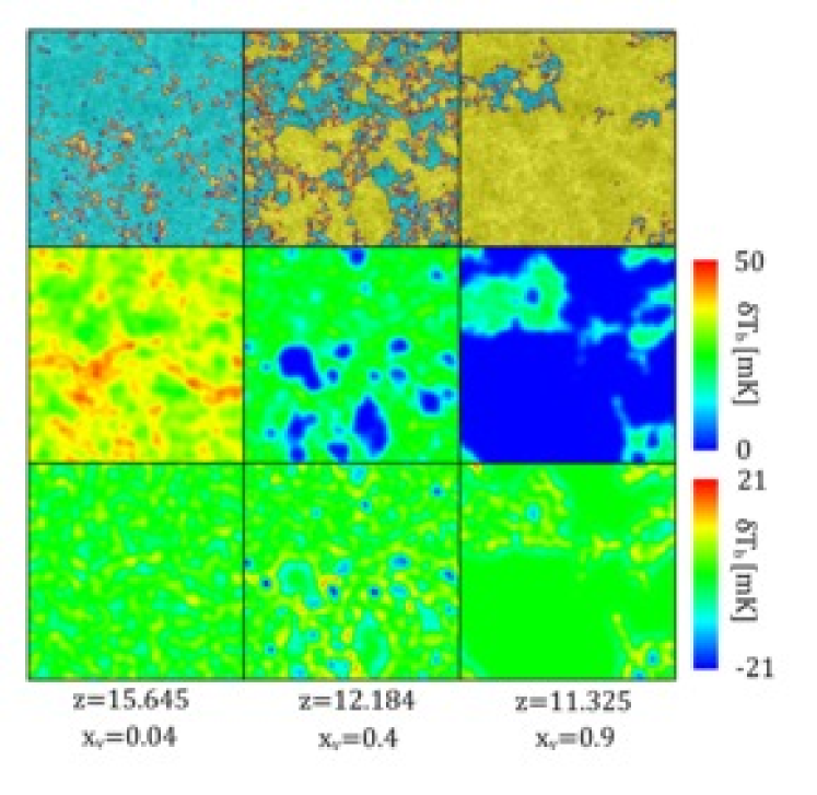
Figure 1: 21-cm maps at redshifts $z=15.645,12.184$ and 11.325 for f125_1000S. Top row: slices which are frequency-averaged into one band of $\Delta\nu=0.2\mathinner{\mathrm{MHz}}$, showing ionized regions (yellow) and neutral regions (blue), superimposed on the density field (light and dark for high-density and low-density regions, respectively). Middle row: corresponding 2D 21-cm differential brightness temperature, averaged by a Gaussian beam of $\Delta\theta=1^{\prime}$. Bottom row: same as middle, but with a compensated Gaussian beam of the same $\Delta\theta$.

Radio signals, observed by radio antennae, should be integrated over the angle, frequency and time in order to achieve the sensitivity required for specific scientific goals. Observing signals from high-redshifts is challenging, especially because these signals are very weak while the required angle- and frequency-resolutions are relatively high. Therefore, very intensive integration in time ($\sim 1000$ hours) is required for EOR observations in general.

We therefore choose the beam size and the frequency bandwidth which we find adequate for generating distinctive 2D genus curves from different reionization scenarios, under the assumption of very long time integration ($\sim 1000$ hours or more). We generated mock 21-cm emission sky maps for our four reionization scenarios, f5, f250, f125_125S and f125_1000S, averaging $\delta T_{b}$ on our computational grid over angle and frequency. First, note that our box size corresponds to the frequency bandwidth

$$\Delta\nu_{\rm box} = \frac{\nu_{0}L_{\rm box}H_{0}\sqrt{\Omega_{m}(1+z)^{3}+\Omega_{\Lambda}}}{c\,(1+z)^{2}}$$ (9)

$$\simeq (4.10\mathinner{\mathrm{MHz}})\mathinner{\left(\frac{L_{\rm box}}{66\mathinner{h^{-1}\,\mathrm{Mpc}}}\right)}\mathinner{\left(\frac{h}{0.719}\right)}$$

$$\times\mathinner{\left(\frac{\Omega_{m}}{0.258}\right)^{1/2}}\mathinner{\left(\frac{1+z}{15}\right)^{-1/2}}\,,$$

and the transverse angle

$$\Delta\theta_{\rm box} = \frac{L_{\rm box}}{(1+z)\mathinner{D_{A}\mathopen{\left(z\right)}}}=\frac{L_{\rm box}}{\mathinner{r\mathopen{\left(z\right)}}}$$ (10)

$$= (30.25\rm arcmin)\mathinner{\left(\frac{L_{\rm box}}{66\mathinner{h^{-1}\,\mathrm{Mpc}}}\right)}$$

$$\times\mathinner{\left(\frac{10563.5-11863.5(1+z)^{-1/2}}{10563.5-11863.5(15)^{-1/2}}\right)^{-1}}$$

where $\nu_{0}\equiv 1420\mathinner{\mathrm{MHz}}$ is the rest frame frequency of the line, $\mathinner{D_{A}\mathopen{\left(z\right)}}$ the angular diameter distance, $L_{\rm box}$ the comoving length of our simulation box, $c$ the speed of light and $H_{0}\equiv 100\,h\mathinner{\mathrm{km}\,\mathrm{s}^{-1}\,\mathrm{Mpc}^{-1}}$ the Hubble parameter at $z=0$. The numerator in the last parenthesis in Equation (10) is a fitting formula for the line-of-sight comoving distance $r(z)$ in units of Mpc, under the cosmological parameters used in this paper.

We first calculate the bare differential brightness temperature on our computational grid by using Equation (5). We then integrated them over frequency with chosen $\Delta\nu$’s. We also consider the Doppler shift due to peculiar velocity. Along the line-of-sight (LOS), the frequency-averaged $\delta T_{b}$ then becomes

$$\langle\delta T_{b}\rangle_{\Delta\nu}=\frac{\sum_{i}(\delta T_{b})_{i}f_{i}}{N_{\Delta\nu}}\,,$$ (11)

where $N_{\Delta\nu}\equiv\mathinner{\Delta L\mathopen{\left(\Delta\nu\right)}}/l_{\rm cell}$ is the number of cells corresponding to $\Delta\nu$ at a given redshift, $f_{i}$ the fraction of a cell $i$ entering the band after the Doppler shift,

$$\mathinner{\Delta L\mathopen{\left(\Delta\nu\right)}} \equiv \frac{\Delta\nu\,c\,(1+z)^{2}}{\nu_{0}H_{0}\sqrt{\Omega_{m}(1+z)^{3}+\Omega_{\Lambda}}}$$ (12)

$$\simeq (3.22\mathinner{h^{-1}\,\mathrm{Mpc}})\mathinner{\left(\frac{\Delta\nu}{0.2\mathinner{\mathrm{MHz}}}\right)}\mathinner{\left(\frac{h}{0.719}\right)^{-1}}$$

$$\times\mathinner{\left(\frac{\Omega_{m}}{0.258}\right)^{-1/2}}\mathinner{\left(\frac{1+z}{15}\right)^{1/2}}\,$$

the comoving length along LOS corresponding to $\Delta\nu$, and $l_{\rm cell}$ the comoving length of a unit cell. For statistical reasons, we generate four 21-cm emission maps for each LOS direction from a single simulation box by periodically shifting the box by a quarter of box size ($L_{\rm box}/4$). These maps will be almost mutually independent, because $L_{\rm box}/4\gg\mathinner{\Delta L\mathopen{\left(\Delta\nu\right)}}$. We also take three different directions for LOS ($x$-, $y$-, and $z$-direction) by rotating the box, such that we have in total 12 (almost) independent 21-cm sky maps from a single simulation box at a given redshift.

Because the shape of the beam varies over different antennae, we choose two different types of beams to average the signal in angle: Gaussian and compensated Gaussian. We first convolve the 21-cm emission map from simulations with a Gaussian filter

$$\mathinner{W_{\rm G}\mathopen{\left(\theta\right)}}=\frac{1}{2\pi\sigma^{2}}\,\mathinner{\exp\mathopen{\left(-\frac{\theta^{2}}{2\sigma^{2}}\right)}}$$ (13)

with a full width at half maximum (FWHM) $\Delta\theta=2\sigma\sqrt{2\ln 2}$. We also use a compensated Gaussian filter given by

$$\mathinner{W_{\rm CG}\mathopen{\left(\theta\right)}}=\frac{1}{2\pi\sigma^{2}}\left(1-\frac{\theta^{2}}{2\sigma^{2}}\right)\mathinner{\exp\mathopen{\left(1-\frac{\theta^{2}}{2\sigma^{2}}\right)}}$$ (14)

with a FWHM given by

$$\Delta\theta=2\sigma\sqrt{2(1-\mathinner{\mathrm{LambertW}\mathopen{\left(e/2\right)}})}$$ (15)

where $\mathinner{\mathrm{LambertW}\mathopen{\left(e/2\right)}}\approx 0.685$.

A Gaussian filter is widely used in the literature to approximate actual beams. In general, an interferometer will not retain the average (large scale) signal, but only record the fluctuations between minimum and maximum angular scales (depending on the largest and smallest baselines). As the largest scales to which the upcoming interferometers are sensitive are larger than our simulated images, a reasonable approach would be to subtract the mean signal from our images. However, for the determination of the genus this does not make a difference other than shifting the threshold value, so we retain the average signal here. A compensated Gaussian filter roughly mimics the beam of a compact interferometer (e.g. Mellema et al., 2006b), even though real beams have sometimes much more complicated shapes depending on the actual configuration of the antenna. We just take $W_{\rm CG}$ as an extreme case for “dirty” beams, clearly distinct from $W_{\rm G}$, because this filter is somewhat pathological as it suppresses both small and large scale features. When $\theta>\sqrt{2}\sigma$, $\mathinner{W_{\rm CG}\mathopen{\left(\theta\right)}}<0$ such that a data field convolved with $\mathinner{W_{\rm CG}\mathopen{\left(\theta\right)}}$ may change its sign from point to point. 21-cm signals filtered this way would show a seemingly unnatural H ii bubble feature, or in the worse case, even absorption signals ($\delta T_{b}<0$), although Equation (5) implies that $\delta T_{b}>0$ when $T_{S}\gg T_{\rm CMB}$.

Figure 1 shows how the actual 2D $\delta T_{b}$ field (top rows) will be observed in different filtering schemes (middle: $W_{\rm G}$; bottom: $W_{\rm CG}$). Three different epochs were chosen to represent early (volume weighted ionized fraction $x_{\rm v}=0.04$), middle ($x_{\rm v}=0.4$), and late ($x_{\rm v}=0.9$) stages. $W_{\rm C}$ generates reasonably filtered $\delta T_{b}$ maps at all the three epochs. At very early ($x_{\rm v}=0.04$) and late ($x_{\rm v}=0.9$) stages, fluctuations in $\delta T_{b}$ are dominated by $1+\delta$ and $1-x$, respectively, while at the middle ($x_{\rm v}=0.4$), both $1+\delta$ and $1-x$ contribute to the fluctuations.

The compensated Gaussian beam adds ripple structures to the emission signals. When a uniform field confined within a certain boundary is convolved with $W_{\rm CG}$, this ripple becomes visible only along the boundary. As the ionized regions grow, therefore, a compensated Gaussian beam produces a negative through of width similar to the beam FWHM at the boundaries of the bubbles. In general, $W_{\rm CG}$ changes the topology of the 21-cm signal. For most of our analysis, therefore, we just use $W_{\rm G}$. Further comparison between these two filters will be made in Section 4.3.2.

4.2 Evolution, Sensitivity, Bubble Distribution, and Power Spectrum

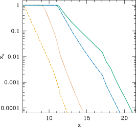
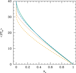
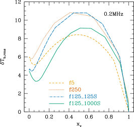
Figure 2: Left: Evolution of the mean volume ionized fraction as a function of redshift. Middle: mean differential brightness temperature with $1\rm arcmin$ FWHM Gaussian beam and $0.2\mathinner{\mathrm{MHz}}$ bandwidth, as a function of the mean volume ionized fraction. Right: rms fluctuation of the differential brightness temperatures filtered by the same beam and bandwidth, as a function of the mean volume ionized fraction.

The evolution of the global volume-weighted ionized fraction $x_{\rm v}$ varies significantly over different reionization scenarios, as seen in Figure 2. First, the end of reionization in the f5 and f250 cases occurs relatively later than in the f125_125S and f125_1000S cases, because these are tied only to high-mass ($M>2\times 10^{9}M_{\odot}$) halos, which collapse much later than low-mass ($10^{8}\lesssim M/M_{\odot}\lesssim 10^{9}$) halos. Second, f5 and f250 also show a steeper evolution in $x_{\rm v}$, because there is no chance for slow evolution of the total luminosity from self-regulation of small-mass halos.

In general, it is a better practice to compare different models at a fixed global ionized fraction rather than at a fixed redshift, partly because there is still too much freedom in the exact epoch of the end of reionization, the time-integrated optical depth to Thompson scattering of CMB photons, etc. More importantly, a fixed global ionized fraction among different models is reached by roughly the same number of H-ionizing photons accumulated from the beginning of the EOR. We therefore use $x_{\rm v}$ as the time indicator of the global evolution throughout this paper.

Using $x_{\rm v}$ as the time indicator, we first observe similar trends in the evolution of $\delta T_{b}$ among different models. The mean differential brightness temperature $\langle\delta T_{b}\rangle$ starts from $\langle\delta T_{b}\rangle\approx 30-40\mathinner{\mathrm{mK}}$ and gradually decreases in time, as seen in Figure 2. The root-mean-square (rms) fluctuation of $\delta T_{b}$, $\delta T_{b,\mathrm{rms}}$, reaches the maximum ($\sim 8-11\mathinner{\mathrm{mK}}$) at $x_{\rm v}\approx 0.4-0.6$ (Figure 2), when the signal is filtered with $\Delta\nu=0.2\mathinner{\mathrm{MHz}}$ and $\Delta\theta=1\rm arcmin$.

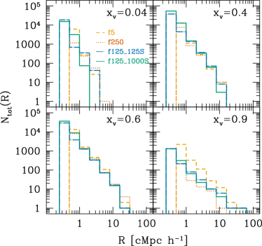
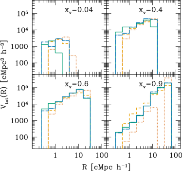
Figure 3: Left: Probability distribution functions of the bubble size. We determined the size of a bubble using the method of Zahn et al. (2006), and select mutually exclusive bubbles using that of Hoyle & Vogeley (2002). Right: volume-weighted probability distribution functions of the bubble size.

Albeit similar trends, a detailed analysis will be needed to discriminate between different models and ultimately probe the properties of the sources. The probability distribution function (pdf) of the bubble size is a useful tool for understanding the impact of these source properties. The bubble size is associated with the mass spectrum of halos and the ionizing efficiency $f_{\gamma}$, simply because it roughly reflects the total number of H-ionizing photons emitted into the bubble. In order to find the pdf of the bubble size, we use a hybrid method. First, the size of a bubble is determined by the method in Zahn et al. (2006): the bubble size is the maximum radius of a sphere from each simulation cell inside which the ionized fraction is over 90%. In this way, every cell in the box is associated with a bubble with a certain size. We then use the void-finding method of Hoyle & Vogeley (2002), which has been extensively used for finding cosmological voids which are mutually exclusive in space. The bubbles are sorted in size from the largest to the smallest. The largest bubble is considered an isolated one. We then move to the next largest bubble and check if there is any overlap in volume with the fist one. We iterate this over the bubble list until the overlap becomes less than 10%, which then registers another isolated bubble. This process is further iterated and we obtain the full list of mutually exclusive bubbles (to the extent of a 10% overlap).

In Figure 3, we show the pdf of the bubble size obtained in this way. We can observe a clear distinction of f5 and f250 from f125_125S and f125_1000S. In f5 and f250, a given ionized fraction is reached only by high-mass halos. For example, to reach $x_{\rm v}\sim 0.6$, the evolutionary stage of cosmological structure formation should enter a highly nonlinear phase because there is only one species (high-mass halos) responsible for such high $x_{\rm v}$. In contrast, in f125_125S and f125_1000S, both the two different species (high- and low-mass halos) contribute to, for example, $x_{\rm v}\sim 0.6$. Therefore, structure formation will be in a less nonlinear stage than the former cases. Correspondingly, we can expect stronger clustering of sources for f5 and f250, and weaker for f125_125S and f125_1000S. Correspondingly, the merger of bubbles would be stronger for the former and weaker for the latter, respectively. This is finally reflected in the relative contribution to a given $x_{\rm v}$ from largest bubbles, as seen in Figure 3. Large bubbles dominate $x_{\rm v}$ in f5 and f250, while there is a relatively smaller contribution to $x_{\rm v}$ in f125_125S and f125_1000S.

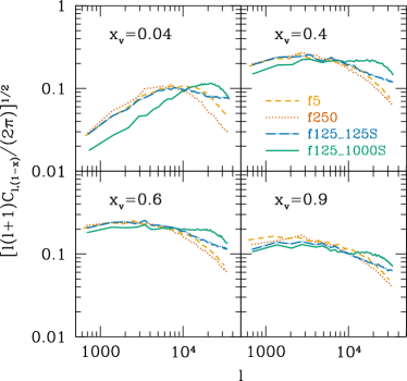
Figure 4: 2D angular power spectra of the neutral fraction $1-x$.

We also obtain 2D angular power spectra of the neutral fraction, $1-x$, for further analysis. This provides insights on the clustering scale of the sources of radiation, or H sc ii bubbles, through the location of peaks in the power spectrum. We follow the convention used in CMB analysis and constructed $[\ell(\ell+1)C_{\ell}/2\pi]^{1/2}$ in spherical harmonics, where $\ell$ roughly corresponds to $2\pi/\theta$ (see Figure 4). At $x_{\rm v}=0.04$, it is clearly seen how cosmic reionization commences in each scenario. f5 and f250 show peaks in $\ell(\ell+1)C_{\ell}$ at $\ell\sim 10^{4}$, or at the comoving length scale $x\sim 6-7\mathinner{h^{-1}\,\mathrm{Mpc}}$, while f125_1000S shows a peak at $\ell\sim 3\times 10^{4}$, or at $x\sim 2\mathinner{h^{-1}\,\mathrm{Mpc}}$, and f125_125S shows a long uniform tail from $\ell\sim 3\times 10^{4}$ to $\ell\sim 4\times 10^{4}$. The behavior of 2D angular power spectra indicates stronger merger of (otherwise) individual bubbles into a larger scale at $x\sim 6-7\mathinner{h^{-1}\,\mathrm{Mpc}}$ in f5, f250 and f125_125S than in f125_1000S. Even though f125_125S has a tail up to $\ell\sim 4\times 10^{4}$ ($x\sim 1\mathinner{h^{-1}\,\mathrm{Mpc}}$), a smaller $f_{\gamma}(=125)$ in small halos than that of f125_1000S ($f_{\gamma}=1000$) makes these small halos less efficient. This is true at all redshifts: the power spectrum of f125_125S is hardly distinguishable from those of f5 and f250 at any time, except for higher power in the smallest length scale (highest $\ell$). In contrast, a distinctive clustering scale, $\ell\sim 3\times 10^{4}$ ($x\sim 2\mathinner{h^{-1}\,\mathrm{Mpc}}$), is shown at all redshifts in f125_1000S, due to the clustering of small halos of the highest efficiency.

In short, both the bubble pdf and the 2D angular power spectrum of the neutral fraction may be useful tools for understanding the nature of different reionization scenarios. In Section 4.3, when we analyze 2D genus curves of different cases, we will characterize these properties to see whether 2D genus curves created from possible observations can show similar fundamental nature as well.

4.3 Genus Properties

We generate $\mathinner{g_{\rm 2D}\mathopen{\left(\delta T_{b}\right)}}$ from selected epochs at which $x_{\rm v}=0.04$, 0.4, 0.6 and 0.9 as described in Section 3. The base 2D field of $\delta T_{b}$ is averaged in frequency with $\Delta\nu=0.2$, 1 and $2\mathinner{\mathrm{MHz}}$, and in angle with $\Delta\theta=1\rm arcmin$, $2\rm arcmin$ and $3\rm arcmin$. We vary $\Delta\nu$ and $\Delta\theta$ to quantify the competing effects of changing resolution and sensitivity, and also to make comparison with characteristics of future radio antennae. In angle-averaging, only $W_{\rm G}$ is used in all the cases, except for f125_1000S where $W_{\rm CG}$ is also applied to understand the impact of the beam shape on $g_{\rm 2D}$.

4.3.1 2D Genus of Density Fluctuations

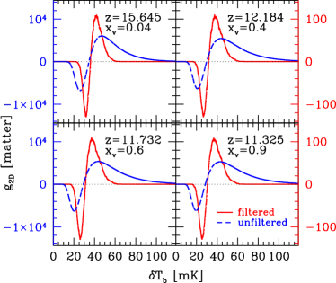
Figure 5: 2D genus defined by the threshold differential brightness temperature within a $\sim 30\rm arcmin\times 30\rm arcmin$ square (corresponding to our box size) in the sky assuming all the gas was neutral, filtered with $1\rm arcmin$ FWHM Gaussian beam and $0.2\mathinner{\mathrm{MHz}}$ bandwidth (red). In comparison, we also show the 2D genus of the differential brightness temperature with the same condition but from one-cell thick slice in our simulation (blue). $\mathinner{g_{\rm 2D}\mathopen{\left(\delta T_{b,n}\right)}}$ of the bare $N$-body field is thus subject to smoothing over the size of the cell. This result is based upon the high-resolution N-body simulation (used for Cases 3 and 4).

Is there any useful template genus curve to be compared with $\mathinner{g_{\rm 2D}\mathopen{\left(\delta T_{b}\right)}}$? There is such a template indeed, namely $g_{\rm 2D}$ of an artificial field of $\delta T_{b}$, which reflects the density fluctuation only. Let us denote this quantity by

$$\delta T_{b,n} \equiv \mathinner{\delta T_{b}\mathopen{\left(x=0\right)}}$$ (16)

$$= (28\mathinner{\mathrm{mK}})\mathinner{\left(\frac{h}{0.719}\right)}\mathinner{\left(\frac{1+z}{10}\right)^{1/2}}$$

$$\times\mathinner{\left(\frac{\Omega_{b}}{0.044}\right)}\mathinner{\left(\frac{\Omega_{m}}{0.258}\right)^{-1/2}}(1+\delta).$$

The distribution of $\delta T_{b,n}$ will be Gaussian in the linear regime ($|\delta|\ll 1$), which will provide a well-defined, analytical $\mathinner{g_{\rm 2D,Gauss}\mathopen{\left(\delta T_{b,n}\right)}}$. Even when $\mathinner{g_{\rm 2D}\mathopen{\left(\delta T_{b,n}\right)}}$ starts to deviate from $\mathinner{g_{\rm 2D,Gauss}\mathopen{\left(\delta T_{b,n}\right)}}$ due to nonlinear evolution of high density peaks, $\mathinner{g_{\rm 2D}\mathopen{\left(\delta T_{b,n}\right)}}$ will be used to indicate overdense ($\delta>0$) and underdense ($\delta<0$) regions. Figure 5 implies that $\delta T_{b,n}>0$ corresponds to $\delta>0$, while $\delta T_{b,n}<0$ to $\delta<0$.

The curve $\mathinner{g_{\rm 2D}\mathopen{\left(\delta T_{b,n}\right)}}$, plotted in Figure 5, shows how the matter density evolves. At $z\approx 10-15$, there already exist extended tails into high $\delta T_{b,n}$, because these correspond to high-density peaks that have evolved into the nonlinear regime. Note that a purely Gaussian random field generates $g_{\rm 2D,Gauss}$, which is symmetrical around $\nu=0$, while high-density peaks (on high $\nu$) that evolved nonlinearly deviate from the Gaussian distribution to make $g_{\rm 2D}$ deviate from $g_{\rm 2D,Gauss}$. Because we will use filtered $\delta T_{b}$ maps, $g_{\rm 2D}$ of filtered $\delta T_{b,n}$ will be the template to be used throughout this paper. Filtering makes both the amplitude and width of $\mathinner{g_{\rm 2D}\mathopen{\left(\delta T_{b,n}\right)}}$ shrink (Figure 5). Nevertheless, even after filtering, regions with positive $g_{\rm 2D}$ correspond to overdense regions and negative $g_{\rm 2D}$ to underdense regions, because the mean-density point (where the $\mathinner{g_{\rm 2D}\mathopen{\left(\delta T_{b,n}\right)}}$ curve crosses the $\delta T_{b}$ axis) is almost unshifted. This will work as a perfect indicator, if comparison is made with $\mathinner{g_{\rm 2D}\mathopen{\left(\delta T_{b}\right)}}$, about how different the $\delta T_{b}$ field is from the underlying density field. $\mathinner{g_{\rm 2D}\mathopen{\left(\delta T_{b,n}\right)}}$ can be obtained accurately for any redshift as long as cosmological parameters are known to high accuracy, which is the case in this era of precision cosmology.

4.3.2 Evolution of $g_{\rm 2D}$ and Beam Shape Impact

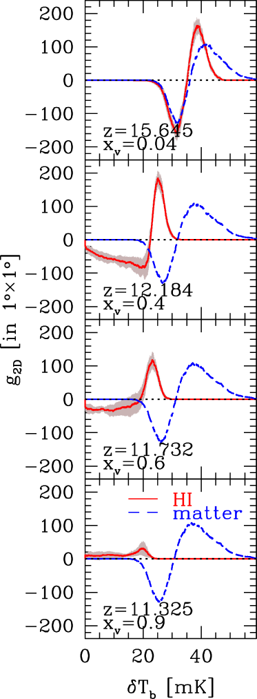
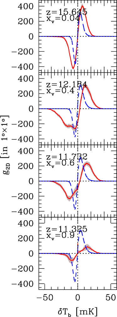
Figure 6: Left: 2D genus of $\delta T_{b}$ for f125_1000S, filtered with a $1\rm arcmin$ FWHM Gaussian beam and $0.2\mathinner{\mathrm{MHz}}$ bandwidth (solid), compared to the template 2D genus out of the underlying density field (dashed), also filtered in the same way. Right: Same as the left panel, but with a compensated Gaussian beam applied.

We found that the evolution of $\mathinner{g_{\rm 2D}\mathopen{\left(\delta T_{b}\right)}}$ contained both generic and model-dependent features. We describe the generic features based on the f125_1000S case. We will describe the model-dependent features in Section 4.3.3.

We find that the change of $\mathinner{g_{\rm 2D}\mathopen{\left(\delta T_{b}\right)}}$ clearly shows how reionization proceeds in time. The left panel of Figure 6 shows $W_{\rm G}$-filtered $\mathinner{g_{\rm 2D}\mathopen{\left(\delta T_{b,n}\right)}}$ of the underlying matter density field (blue dashed line) and $\mathinner{g_{\rm 2D}\mathopen{\left(\delta T_{b}\right)}}$ of the differential brightness temperature field of the HI gas (red line). In the earliest phase of reionization ($x_{\rm v}=0.04$), $\mathinner{g_{\rm 2D}\mathopen{\left(\delta T_{b}\right)}}$ is much smaller than $\mathinner{g_{\rm 2D}\mathopen{\left(\delta T_{b,n}\right)}}$ at high temperature thresholds ($\delta T_{b,n}\gtrsim 50\mathinner{\mathrm{mK}}$). It is because the highest density peaks have been ionized by the sources inside them, and are dropped out of the neutral gas distribution. It can also be noted that the amplitudes of both the maximum (at $\delta T_{b}\sim 38\mathinner{\mathrm{mK}}$) and minimum (at $\delta T_{b}\sim 33\mathinner{\mathrm{mK}}$) of $\mathinner{g_{\rm 2D}\mathopen{\left(\delta T_{b}\right)}}$ are higher than those of $\mathinner{g_{\rm 2D}\mathopen{\left(\delta T_{b,n}\right)}}$. The birth of new islands and peninsulas made of H I regions — some peninsulas may appear as islands at certain $\delta T_{b,\mathrm{th}}$ — is responsible for the former, while the birth of new lakes made of H II regions is responsible for the latter. The birth of islands and peninsulas occurs at mildly overdense regions ($\delta T_{b,n}\sim 38\mathinner{\mathrm{mK}}$) because bubbles are clustered such that some of them merge with one another to fully or partly surround neutral regions. Note that a neutral region identified as an island in 2D may well be a cross-section of a vast neutral region in 3D.

When the Universe enters the intermediate phase of reionization ($x_{\rm v}\approx 0.4-0.6$), almost all overdense regions ($\delta T_{b,n}\gtrsim 30\mathinner{\mathrm{mK}}$) have been ionized to form larger bubbles. This is reflected in the relatively low amplitude trough of $\mathinner{g_{\rm 2D}\mathopen{\left(\delta T_{b}\right)}}$, which appears in very low-density ($\delta T_{b,n}\lesssim 20\mathinner{\mathrm{mK}}$) regions. Now many more islands appear in mildly underdense ($\delta T_{b,n}\sim 25\mathinner{\mathrm{mK}}$) regions because larger and more clustered bubbles penetrate further into the low-density IGM and are more efficient in forming new islands. As time passes from $x_{\rm v}=0.4$ to $x_{\rm v}=0.6$, the amplitude of $g_{\rm 2D}$ decreases as bubbles merge with each other and neutral clumps disappear. Further penetration of bubbles into the lower-density IGM from $x_{\rm v}=0.4$ to $x_{\rm v}=0.6$ is also reflected in the maximum value of $\delta T_{b}$ for nonzero $\mathinner{g_{\rm 2D}\mathopen{\left(\delta T_{b}\right)}}$.

Finally, in the late stage ($x_{\rm v}=0.9$), all ionized bubbles have been connected and the last surviving neutral clumps exist to give positive $g_{\rm 2D}$ at $\delta T_{b}\sim 20\mathinner{\mathrm{mK}}$. Note that these clumps exist only in underdense regions, which is a clear indication of the fact that reionization proceeds in an inside-out fashion: high-density regions will be ionized first due to the proximity to the sources of radiation, and low-density regions will be ionized later.

We then briefly investigate the impact of beam shapes. The impact of $W_{\rm CG}$ on $g_{\rm 2D}$ is demonstrated on the right panel of Figure 6. Note that the Fourier transform of $W_{\rm CG}$ is proportional to $k^{2}\sigma^{2}\exp(-k^{2}\sigma^{2}/2)$. From the convolution theorem, it is obvious that the filtered field becomes the $W_{\rm G}$-smoothed, negative Laplacian ($-\nabla^{2}$) of the field. Note that Laplacian is equivalent to the divergence of the gradient. Therefore, if the $\delta T_{b}$ field is filtered by $W_{\rm CG}$, $\delta T_{b}$s in those regions with the steepest spatial gradient in $x$ or $\delta$ will correspond to extrema. We also note that the sign of the Laplacian depends on the morphology of $x$: if H II bubbles form in the sea of neutral gas, gradients of $\delta T_{b}$ diverge ($-\nabla^{2}\delta T_{b}<0$), while if neutral clumps remain in the sea of ionized gas, gradients of $\delta T_{b}$ converge ($-\nabla^{2}\delta T_{b}>0$). An interesting feature in $\mathinner{g_{\rm 2D}\mathopen{\left(\delta T_{b}\right)}}$ is indeed observed to move from regions with $\delta T_{b}<0$ at a relatively early ($x_{v}\sim 0.4$) stage to regions with $\delta T_{b}>0$ at a later ($x_{v}\sim 0.9$) stage. Nevertheless, because the topology of the 21-cm signal is processed further (Gaussian smoothing and Laplacian) in the case of $W_{\rm CG}$ than that of $W_{\rm G}$ (Gaussian smoothing only), the interpretation becomes less transparent. We also note that $W_{\rm CG}$ filters out almost all the scales except for the filtering scale, while $W_{\rm G}$ filters out only scales smaller than the filtering scale.

The nice interpretative power of $\mathinner{g_{\rm 2D}\mathopen{\left(\delta T_{b}\right)}}$ is somewhat lost with $W_{\rm CG}$. Based on this, we suggest that any artificial effects from “dirty” beams should be removed or minimized in real observations. Only when the effective beam shape becomes something close to $W_{\rm G}$, general analyses including our genus method will exploit their full potential.

4.3.3 Model-Dependent Feature and Required Sensitivity

We finally investigate whether our 2D genus analysis can discriminate between different reionization scenarios. Ultimately, if this turns out to be true, we may be able to probe properties of radiation sources at least indirectly, because these properties determine how cosmic reionization proceeds.

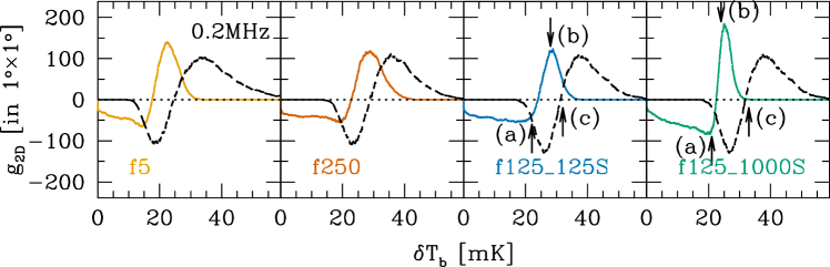
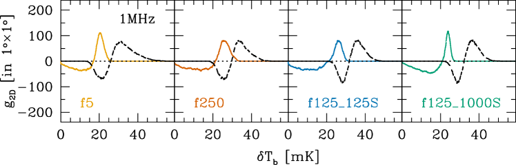
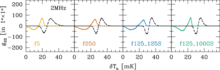
Figure 7: 2D genus curves of the differential brightness temperatures at $x_{v}=0.4$, filtered with a $1\rm arcmin$ FWHM Gaussian beam and with $0.2\mathinner{\mathrm{MHz}}$ (top), $1\mathinner{\mathrm{MHz}}$ (middle), $2\mathinner{\mathrm{MHz}}$ (bottom) bandwidth; the curves are compared with those of the matter densities (black).

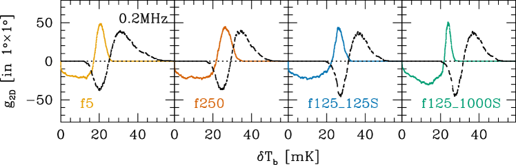
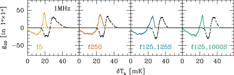
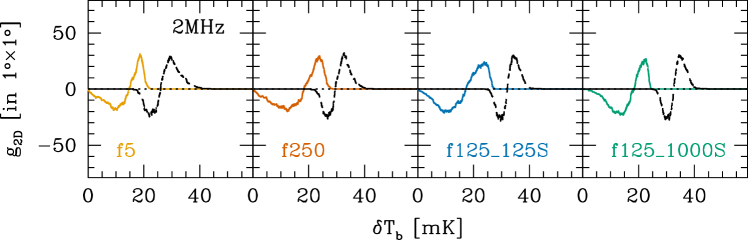
Figure 8: Same as Figure 7, but with a $2\rm arcmin$ FWHM Gaussian beam applied.

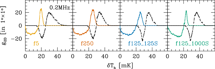
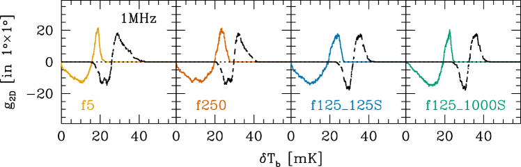
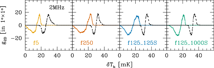
Figure 9: Same as Figure 7, but with a $3\rm arcmin$ FWHM Gaussian beam applied.

$\begin{array}[]{lcccc}\textrm{\Large f125\_1000S}&\includegraphics[width=86.72267pt]{fig10a_g125_1000_lower_peak.eps}&\includegraphics[width=86.72267pt]{fig10b_g125_1000_upper_peak.eps}&\includegraphics[width=86.72267pt]{fig10c_g125_1000_zero_matter.eps}&\includegraphics[width=86.72267pt]{fig10d_density_g125_1000.eps}\\ \textrm{\Large f125\_125S}&\includegraphics[width=86.72267pt]{fig10e_g125_125_lower_peak.eps}&\includegraphics[width=86.72267pt]{fig10f_g125_125_upper_peak.eps}&\includegraphics[width=86.72267pt]{fig10g_g125_125_zero_matter.eps}&\includegraphics[width=86.72267pt]{fig10h_density_g125_125.eps}\\[8.61108pt] &\textrm{\Large a}&\textrm{\Large b}&\textrm{\Large c}&\textit{\Large x}\\ \end{array}$

Figure 10: How the 2D genus depends on reionization scenarios: from left to right, threshold $\delta T_{b}$’s (contour lines) are selected, in order to obtain the minimum $g_{\rm 2D}(\delta T_{b})$, maximum $g_{\rm 2D}(\delta T_{b})$, and zero $g_{\rm 2D}(\delta T_{b,n})$, respectively, along with the snapshot of the unfiltered ionized fraction (far right). $x_{v}=0.4$ in both (top: f125_1000S; bottom: f125_125S) cases. See the arrows in Figure 7 for the contours a, b and c.

Our 2D genus analysis seems very promising, indeed, in probing source properties. The top panel in Figure 7 shows $g_{\rm 2D}(\delta T_{b})$ and $g_{\rm 2D}(\delta T_{b,n})$ for all cases at $x_{\rm v}=0.4$. The impact of small-mass ($10^{8}\lesssim M/M_{\odot}\lesssim 10^{9}$) halos is observed as follows. In f125_1000S, almost all the (filtered) overdense regions have been ionized at this epoch due to efficient, small-mass halos. In contrast, when there are no small-mass halos (f5, f250) or if small-mass halos are not as efficient (f125_125S), some fraction of overdense regions still remains neutral at $x_{\rm v}\sim 0.4$. These regions are mildly nonlinear, and are ionized due to the almost on-the-spot existence of efficient small-mass halos in f125_1000S, while they mostly remain neutral or only partially ionized in f5, f250 and f125_125S due to the absence or low-efficiency of small-mass halos (Figure 10). The relatively larger amplitude of $g_{\rm 2D}$ in f125_1000S is the reflection that there are many more small individual islands and bubbles, as explained in Section 4.3.2.

The impact of beam size and bandwidth is shown in Figures 7–9. As the applied $\Delta\nu$ increases, the $g_{\rm 2D}$ curve shrinks in width and moves toward the left. The interpretation we made on f125_1000S with $\Delta\nu=0.2\,{\rm MHz}$ and $\Delta\theta=1^{\prime}$ somewhat weakens, in the sense that $g_{\rm 2D}$ curves are mapped too deep in the (newly filtered) underdense regions. Nevertheless, the amplitude of $g_{\rm 2D}$ is the largest and the rightmost wing of $g_{\rm 2D}$ is located at the smallest $\delta T_{b}$ in f125_1000S in all the varying filtering scales, just as when $\Delta\nu=0.2^{\prime}{\rm MHz}$ is applied.

Since $g_{\rm 2D}$ is a useful tool for understanding the evolution (Section 4.3.2) and even for discriminating between reionization scenarios, we need to ask whether this can be achieved in real observations. To estimate the required sensitivity, we show the degree of fluctuation in filtered $\delta T_{b}$ in Figure 11. $\delta T_{b,\,\rm rms}$ becomes maximum around the middle stage of the reionization in all the cases. Roughly speaking, $\delta T_{b,\,\rm rms}$ gives the required rms sensitivity limit of a radio antenna in each configuration, which is around a few mK.

$\begin{array}[]{ccc}\includegraphics[width=125.74689pt]{fig11a_sens1.eps}&\includegraphics[width=125.74689pt]{fig11b_sens2.eps}&\includegraphics[width=125.74689pt]{fig11c_sens3.eps}\\ \includegraphics[width=130.08731pt]{fig11d_rms_0p2mhz.eps}&\includegraphics[width=130.08731pt]{fig11e_rms_2min_0p2mhz.eps}&\includegraphics[width=130.08731pt]{fig11f_rms_3min_0p2mhz.eps}\\ \includegraphics[width=130.08731pt]{fig11g_rms_1mhz.eps}&\includegraphics[width=130.08731pt]{fig11h_rms_2min_1mhz.eps}&\includegraphics[width=130.08731pt]{fig11i_rms_3min_1mhz.eps}\\ \includegraphics[width=130.08731pt]{fig11j_rms_2mhz.eps}&\includegraphics[width=130.08731pt]{fig11k_rms_2min_2mhz.eps}&\includegraphics[width=130.08731pt]{fig11l_rms_3min_2mhz.eps}\\ \end{array}$

Figure 11: Top row: sensitivity limit of SKA in terms of bandwidth $\Delta\nu$, with varying integration time (100, 1000 and 10000 hours). Also plotted are the required sensitivity limits (cross) for useful results, at $\Delta\nu=0.2$, 1 and 2 MHz. Each column displays a different beam size $\Delta\theta$’s (top labels). Remaining rows: evolution of the rms differential brightness temperature as a function of $\Delta\theta$ (each column) and $\Delta\nu$ (each row).

Following Iliev et al. (2003), we estimate the sensitivity limit of SKA for the filtering scale treated in this paper, to figure out the feasibility of our analysis on real 21-cm background data. We assume the core size to be $\sim 1\,{\rm km}$ for SKA. We also assume, just for the sake of sensitivity estimation, that $x_{\rm v}\sim 0.5$ is reached at $z\sim 8$. Even though our choice of input parameters (properties of the sources) made reionization ending much earlier than the standard end of reionization epoch ($z\sim 6.5$), except for f5, we may imagine that similar distinctive features among different models would still exist if we tuned these parameters to make these models achieve the half-ionized state at $z\sim 8$. Figure 11 shows the estimated sensitivity under these conditions. Due to the strong dependence of the sensitivity on $\theta$, $\sim\Delta\theta^{-2}$, an increase in the beam size quickly makes our analysis feasible. This comes at a price that values of $g_{\rm 2D}(\delta T_{b})$ shrink further, and the range of $\delta T_{b}$ shifts more to the left. At any rate, $\sim 1000-10000$ hours of integration at $\delta\nu\sim 1-2$ MHz and $\delta\theta\sim 2^{\prime}-3^{\prime}$ seem possible to allow for our analysis.

5 Summary and discussion

We calculated the 21-cm radiation background from high redshift using a suite of structure formation and radiative transfer simulations with different properties of the sources of radiation. These properties are specified by the spectrum of halo masses capable of hosting the sources of radiation and the emissivity of hydrogen-ionizing photons. Assuming the pre-reionization heating of the IGM, we calculated the 21-cm radiation background in the saturated limit, $T_{\rm S}\gg T_{\rm CMB}$, such that its differential brightness temperature is proportional to the underlying density and neutral fraction.

In order to understand the topology of the high-redshift IGM, we developed 2D genus method applicable to the 21-cm radiation background. Basically, this method calculates the 2D genus, the difference between the number of hot and cold spots, under a given threshold differential brightness temperature. We construct 2D genus curves at different redshifts for different scenarios, by varying this threshold values.

We found that the 2D genus curve $\mathinner{g_{\rm 2D}\mathopen{\left(\delta T_{b}\right)}}$, if compared to the $g_{\rm 2D}$ of the underlying density fluctuation $\mathinner{g_{\rm 2D}\mathopen{\left(\delta T_{b,n}\right)}}$, clearly shows the evolution of the reionization process. The $\mathinner{g_{\rm 2D}\mathopen{\left(\delta T_{b}\right)}}$ curve is found to deviate quickly from the $g_{\rm 2D}$ of a Gaussian random field, qualitatively in agreement with the findings of Iliev et al. (2006) and in contrast with the findings of Shin, Trac & Cen (2008). Shin, Trac & Cen (2008) find that the non-Gaussianity of the H II region is small, even when the Universe is 50% ionized. It is also shown that the reionization proceeds in an inside-out fashion: high-density regions get ionized first and low-density regions later.

We also showed that our 2D genus method can be used to discriminate between various reionization scenarios, thus probing the properties of the sources indirectly. It appears to be most effective in discriminating the mass spectra of halos which host the sources of radiation. A hybrid mass spectrum with a different emissivity in different species (f125_1000S in this paper) stands out from the cases with a single species (f5, f250) or a case with equal-emissivity among different species (f125_125S).

Crucial ingredients needed for this analysis are beam shapes and the sensitivity. We tested two different beams, a Gaussian and a compensated Gaussian. The Gaussian beam, even after the field is filtered and degraded, leaves a distinguishable imprint on the 2D genus curve such that different reionization scenarios can be discriminated. In contrast, the compensated Gaussian beam somewhat loses the interpretative power that the Gaussian beam had. Assuming that the compensated Gaussian beam represents the so-called dirty beams, our analysis may be applied entirely only when those artificial effects from dirty beams are removed.

We predict that SKA will be able to produce data suitable for this analysis, when $1000-10000$ hours of integration are performed with $\delta\nu\sim 2-3\,{\rm MHz}$ and $\delta\theta\sim 2^{\prime}-3^{\prime}$ at an observing frequency of $\sim 150\,{\rm MHz}$. Therefore, our method seems promising. Note, however, that a direct link from the observed 2D genus curve to the true properties of the sources will be still far-fetched, when we adopt such low-resolution filters to increase the sensitivity. Moreover, there are still too many uncertainties, such as the matter power spectrum at small scales, which is relevant to the formation and evolution of the sources of reionization. We hope to see many more useful constraints on cosmic reionization from other various, direct or indirect, observations. In the future, we will explore more reionization scenarios to strengthen the potential of our 2D genus analysis.

One caveat of our work is that the simulation box is relatively small, while a $\gtrsim 100$ Mpc box is likely to provide a more statistically reliable result. While 2D genus should be dominated by the most abundant H II bubbles, which are also the smallest bubbles, the cosmic variance guarantees that some bubble sizes, at late stages of reionization, will become larger than the box we used in this work. We have indeed simulated reionization in a very large box ($425/h$ Mpc) and observed a variation of the observational properties (e.g. 3D power spectrum) in a certain range of scales and reionization stages (Iliev et al., 2013). We did not yet analyze the minihalo-included simulation (Ahn et al., 2012), which forms another important class of models with very small H II regions. We thus plan to apply our 2D genus analysis to these new results (more model dependency and bigger box size) and provide a more statistically reliable result which can be used to analyze future 21-cm observations.