The Photon Dispersion as an
Indicator for New Physics ?

Abstract

We first comment on the search for a deviation from the linear photon dispersion relation, in particular based on cosmic photons from Gamma Ray Bursts. Then we consider the non-commutative space as a theoretical concept that could lead to such a deviation, which would be a manifestation of Lorentz Invariance Violation. In particular we review a numerical study of pure $U(1)$ gauge theory in a 4d non-commutative space. Starting from a finite lattice, we explore the phase diagram and the extrapolation to the continuum and infinite volume. These simultaneous limits — taken at fixed non-commutativity — lead to a phase of broken Poincaré symmetry, where the photon appears to be IR stable, despite a negative IR divergence to one loop.

1 Lorentz Invariance

Lorentz Invariance is a central concept of relativity: it is a global symmetry in Special Relativity, and a local symmetry in General Relativity. Here we stay within the framework of particle physics as described by quantum field theory, so we refer to Special Relativity. Then this symmetry implies that some field $\Phi$ (scalar, spinor, vector or tensor) transforms globally in some representation $D$ of the Lorentz group $SO(1,3)$,

$$\Phi(x)\to U(\Lambda)^{\dagger}\Phi(x)U(\Lambda)=D(\Lambda)\Phi(\Lambda^{-1}x)\qquad(\Lambda\in SO(1,3)\ ,\ U{\rm~{}unitary})\ .$$ (1)

A number of high precision tests of Lorentz Invariance involve cosmic rays, see e.g. Refs. LIVrev for recent reviews. They provide perhaps the best chance to probe parameters not that far below the Planck scale (in specific cases even exceeding it). Cosmic rays attain by far the highest particle energies in the Universe (up to $\approx 10^{20}~{}{\rm eV}$). In addition, the fact that they travel over tremendous distances may be conclusive for high precision properties even at moderate or low energies, because tiny effects could be accumulated over a very long trajectory. In view of the latter scenario, we discuss here the photon dispersion relation, as a direct kinematic test of Lorentz Invariance.

2 Cosmic $\gamma$-rays

Gamma Ray Bursts (GBRs) are emitted in powerful energy eruptions over short periods, typically a few seconds or minutes. Temporarily this causes the brightest spots in the sky. They were discovered from satellites since the 70s, but nowadays they can also be observed from ground. Their sources are small, and there are speculations that they could be generated by the merger of neutron stars, or of black holes. Here we are pragmatic about their origin: in any case GRBs exist, and we want to see what we can learn from the long journey of their photons through the Universe.

The distance to the source is usually well evaluated from the redshift (if we assume the Hubble parameter $H_{0}$ to be known). In particular, in the year 2005 a spectacular GRB was observed swift : it occurred at a distance of $3.9~{}{\rm Gpc}$, i.e. it was emitted when the Universe was only $\approx 8\cdot 10^{8}$ years old. Typically the photon energies are in the range of $10^{4}\dots 10^{8}~{}{\rm eV}$. Thus it is an obvious idea to use GRBs to probe if the speed of photons is really energy independent Camel1 .

A systematic study of this question was performed in Ref. Ellis . It probed the effective dispersion ansatz

$$\vec{p}^{\,2}=E^{2}\Big{(}1+\frac{E}{M}\Big{)}\ ,\quad v(E)=1-\frac{E}{M}+{\cal O}\Big{(}\frac{E^{2}}{M^{2}}\Big{)}\ ,$$ (2)

where $M$ is a very heavy mass parameter, which might emerge somehow from some kind of “quantum gravity foam”. Here we set the speed of light at photon energy $E\ll|M|$ to $c=1$. If a finite parameter $M$ exists, deviations of the group velocity $v$ from that speed should be manifest at very high energy $E$, or after a very long path. Ref. Ellis analyzed data of 35 GRBs, detected by three satellites. In fact, photons of higher energy tend to arrive slightly later. This could be explained by a relative delay at the source, $\Delta_{\rm source}$, which would then be amplified by the redshift $z$ to the observed delay $\ \Delta_{\rm obs}=\Delta_{\rm source}(1+z)\,.$ So far this is standard physics. If one includes a finite parameter $M$, this formula is modified to

$$\frac{\Delta_{\rm obs}}{1+z}=\Delta_{\rm source}+a_{\rm LIV}K(z)\ ,\quad a_{\rm LIV}=\frac{\Delta E}{MH_{0}}\ ,$$ (3)

for photon energies that differ by $\Delta E$. Here $a_{\rm LIV}$ is the Lorentz Invariance Violation (LIV) parameter, and the function $K(z)$ is specified in Ref. Ellis . The question is now whether or not the data for $\Delta_{\rm obs}/(1+z)$ are compatible with a constant in $z$ (or $K(z)$). The authors of Ref. Ellis enhanced the errors by hand until the data became compatible with a linear fit. The resulting fit is in fact almost constant, and it suggests

$$|M|>1.4\cdot 10^{25}~{}{\rm eV}\approx 0.001~{}M_{\rm Planck}\quad({\rm with}~{}95~{}\%~{}{\rm C.L.})\ .$$ (4)

Some studies of single GRBs or blazar flares even conclude $|M|\mathop{\raise 1.29167pt\hbox{$>$\kern-7.5pt\raise-4.73611pt\hbox{$\sim$}}}0.01~{}M_{\rm Planck}$ LIVrev . All these results are negative regarding the hope to discover new physics, but it is impressive that phenomenological information about this energy regime is accessible at all.

Further hypothetical LIV effects, that are searched for in cosmic photons, are a decay $\gamma\to e^{+}+e^{-}$, photon splitting, vacuum birefringence and an irregular threshold energy for long distance propagation through the cosmic background radiation LIVrev .

3 $U(1)$ gauge theory in an non-commutative space

Here we address $U(1)$ gauge theory in an non-commutative (NC) space as one specific theoretical framework that could lead to a non-linear photon dispersion relation. Due to its discontinuous behavior in the IR limit, this approach does not belong to the large class of low energy effective actions — such effective LIV theories, including their predictions for photons, have also been reviewed in Refs. LIVrev . Conceptual issues related to causality and energy positivity are discussed in Ref. Ralf .

To describe our framework, let us start by considering a NC Euclidean plane. The (Hermitian) position operators obey the commutation relation

$$[\hat{x}_{\mu},\hat{x}_{\nu}]={\rm i}\Theta_{\mu\nu}={\rm i}\theta\epsilon_{\mu\nu}\qquad(\mu,\nu=1,2)\ ,$$ (5)

where we assume the non-commutativity parameter $\theta$ to be constant. This implies a spatial uncertainty relation $\Delta x_{1}\Delta x_{2}={\cal O}(\theta)$. In a Gedankenexperiment, Ref. DFR interpreted this relation (in $d=4$) as the event horizon, when one tries to measure extremely short distances (of the order of the Planck length), which requires an enormous energy concentration in this range. Thus $\sqrt{\|\Theta\|}$ could be viewed as a “minimal length”, i.e. an additional constant of Nature (similar to the parameter $1/M$ in Section 2).

A field theory on such a space is non-local. On the quantum level, the modification of the standard geometry at short distances implies not only UV, but also IR effects — in particular perturbation theory is in deep trouble due to the emergence of a new type of IR divergences (“UV/IR mixing”) UVIR .

Here we consider a fully non-perturbative approach, which is even more motivated than in commutative quantum field theory. In analogy to that case, we impose a (fuzzy) lattice structure of spacing $a$ by means of the operator identity

$$\exp\Big{(}{\rm i}\frac{2\pi}{a}\hat{x}_{\mu}\Big{)}=\hat{1}\!\!\!1\ .$$ (6)

The momentum components $p_{\mu}$ commute, and they obey the usual periodicity over the Brillouin zone, which implies

$$e^{{\rm i}p_{\mu}\hat{x}_{\mu}}=e^{{\rm i}(p_{\mu}+2\pi/a)\hat{x}_{\mu}}\ \Rightarrow\ \hat{1}\!\!\!1=e^{{\rm i}(p_{\mu}+2\pi/a)\hat{x}_{\mu}}e^{-{\rm i}p_{\nu}\hat{x}_{\nu}}=\dots=\hat{1}\!\!\!1\exp\Big{(}\frac{{\rm i}\pi}{a}\theta(p_{2}-p_{1})\Big{)}\ .$$

At fixed $\theta$ and $a$, this means that the momenta are discrete, and the lattice is automatically periodic. This is of course in contrast to the commutative space. If the lattice is $N\times N$ periodic, the momentum components take the form

$$p_{\mu}=\frac{2\pi}{aN}\,n_{\mu}\quad(n_{\mu}\in\mathbb{Z})\quad\Rightarrow\quad\theta=\frac{1}{\pi}Na^{2}\ .$$ (7)

Therefore the Double Scaling Limit

$$\{a\to 0\quad{\rm and}\quad N\to\infty\}\quad{\rm at}\quad Na^{2}={\rm const.}$$ (8)

leads to a continuous NC plane of an infinite extent. We start from a finite lattice, where both the UV and the IR sector are regular, and we simultaneously remove both regularizations in a controlled manner. Other procedures could easily lead to $\theta\to 0$ or $\theta\to\infty$, which are different commutative limits. The requirement to link the UV and IR extrapolations is related to the notorious UV/IR mixing (for a review, see Ref. Szabo ).

A Fourier-type analysis shows that we can return to the use of ordinary coordinates $x_{\mu}$, if all field multiplications are turned into star products, such as

$$\phi(x)\star\psi(x):=\phi(x)\exp\Big{(}\frac{\rm i}{2}\mathop{\raise 6.02773pt\hbox{$\leftarrow$\kern-7.5pt\raise-6.02773pt\hbox{$\partial$}}}\ \!\!\!_{\mu}\,\theta\,\epsilon_{\mu\nu}\!\mathop{\raise 6.02773pt\hbox{$\rightarrow$\kern-7.5pt\raise-6.02773pt\hbox{$\partial$}}}\ \!\!\!_{\nu}\Big{)}\psi(x)\ .$$ (9)

The $\star$-commutator $[x_{\mu},x_{\nu}]_{\star}:=x_{\mu}\star x_{\nu}-x_{\nu}\star x_{\mu}={\rm i}\Theta_{\mu\nu}$ makes this formulation plausible.

Hence the action of pure $U(1)$ gauge theory on a NC plane can be written as

$$S[A]=\frac{1}{2}\int d^{2}x\,F_{\mu\nu}\star F_{\mu\nu}\ ,\quad F_{\mu\nu}=\partial_{\mu}A_{\nu}-\partial_{\nu}A_{\mu}+{\rm i}g(A_{\mu}\star A_{\nu}-A_{\nu}\star A_{\mu})\ .$$ (10)

This action is $\star$-gauge invariant (though this does not hold for $F_{\mu\nu}$). Note that non-commutativity brings in a Yang-Mills type self-interaction term.

At first sight, it looks hopeless to put this action on a lattice and simulated it: this seems to require $\star$-unitary link variables, $U_{x,\mu}^{\dagger}\star U_{x,\mu}=1\!\!\!1$ (no sum), which can only be constructed and updated with stringent constraints given by the complete configuration. There is a way out, however, namely the mapping onto a matrix model.

A long time ago, and in a different context, González-Arroyo and Okawa introduced the twisted Eguchi-Kawai (TEK) model GAO . It is formulated on a single point, with the action

$$S_{\rm TEK}[U]=N\beta\sum_{\mu\neq\nu}Z_{\mu\nu}{\rm Tr}[U_{\nu}^{\dagger}U_{\mu}^{\dagger}U_{\nu}U_{\mu}]\qquad(\beta=1/g^{2})\ ,$$ (11)

where $U_{\mu}$ ($\mu=1,2$ in $d=2$) are unitary $N\times N$ matrices (which emerged from link variables after dimensional reduction of $U(N)$ lattice gauge theory), and $Z_{21}=Z_{12}^{*}=\exp(2\pi{\rm i}n/N)$ is the twist factor ($n\in\mathbb{Z}$, $n~{}{\rm mod}~{}N\neq 0$). Much later it turned out that this model is equivalent to NC $U(1)$ gauge theory on a $N\times N$ lattice: in particular the algebras were shown to be identical (Morita equivalence) Morita .

Referring to the historic interpretation of the matrices as contracted link variables, it is obvious to formulate (rectangular) Wilson loops in the TEK model as

$$W_{\mu\nu}(I\times J)=\frac{1}{N}\,Z_{\mu\nu}^{I\cdot J}\,{\rm Tr}[U_{\nu}^{\dagger~{}J}U_{\mu}^{\dagger~{}I}U_{\nu}^{J}U_{\mu}^{I}]\ .$$ (12)

Mapping this term back to the NC gauge theory leads to a sensible definition of a NC Wilson loop Wloop . (There are no “closed loops” on a NC plane, but the essential criterion is $\star$-gauge invariance). A specific Wilson loop is complex in general, but the property $W_{\mu\nu}=W_{\nu\mu}^{*}$ guarantees that the action is real positive, since it involves a sum over both plaquette orientations. Therefore the TEK model formulation is suitable for Monte Carlo simulations, i.e. for a non-perturbative study of NC gauge theory.

4 The fate of the non-commutative photon

Let us now address the question how a possible non-commutativity could deform the photon dispersion relation. A 1-loop result of the form

$$E^{2}=\vec{p}^{\,2}+\frac{Cg^{2}}{(p\Theta)^{2}}\qquad(C={\rm const.})$$ (13)

was first derived in Ref. MST . Hence one could even be tempted to deduce a lower bound on $\|\Theta\|$ from the observed high-precision linear dispersion relation (if $\Theta\neq{\bf 0}$) CamelNC . However, further calculations revealed that the constant $C$ is actually negative, $C=-2/\pi^{2}$ LLT . This apparent IR instability is worrisome indeed: it seemed questionable if NC QED does have a ground state, i.e. if it actually represents a well-defined quantum theory. Hence people quickly proceeded to a supersymmetric version of this model, where the negative IR divergence is cancelled LLT . (It is not visible either, of course, when one treats the model classically Rivelles .)

However, we were not happy with this combination of daring hypotheses, so we did not assume supersymmetry in addition. We wanted to verify if the NC photon as such is really ill-defined NCQED . To this end, we considered a “minimally” NC Euclidean space-time, which involves a NC plane, $[\hat{x}_{1},\hat{x}_{2}]={\rm i}\theta={\rm const.}$, plus a commutative plane $(x_{3},t)$ which includes the Euclidean time $t$. (A NC time coordinate would break reflection positivity, so in that case the transition to the Minkowski signature would no be on safe grounds OSax . Commutative time also alleviates the problems with causality.)

For the commutative plane we used the standard regularization of an $L\times L$ lattice, while the NC plane was treated with a TEK model as described in Section 3, i.e. we put a $N\times N$ matrix model on each of the $L^{2}$ lattice sites ($L\approx N$). The first challenge for the numerical measurements was the identification of a scale, in order to define the Double Scaling Limit (8). A simple ansatz for the lattice spacing, $a\propto 1/\beta$, was successful. It corresponds to a Double Scaling Limit which keeps the ratio $N/\beta^{2}$ constant. Fig. 1 illustrates, for the example $N/\beta^{2}=20$, that the Wilson loops $\langle W_{\mu\nu}\rangle$ of different sizes, in various planes, are in fact stable as we vary $N$ and $\beta$ accordingly.

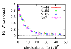
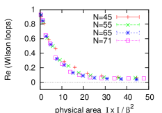
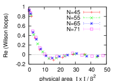
Figure 1: The real part of square-shaped Wilson loops at a constant ratio $N/\beta^{2}=20$. We show results in the commutative plane (left), a mixed plane (center) and the NC plane (right). In the former two planes the Wilson loops are real due to the symmetry in the signs of $x_{3}$ and $t$. In the NC plane $\langle W_{12}\rangle$ has a complex phase which rises linearly in the area for large loops. (This Aharonov-Bohm-type effect was also observed in 2d NC $U(1)$ gauge theory 2dNCU1 , though with some shape dependence of the Wilson loop expectation values BBT .) In all cases we observe an excellent Double Scaling behavior.

Next we measured the open Wilson lines $P_{\mu}(n)$ in $\mu$-direction of length $n$ in lattice unit. In dimensional units this line follows the vector

$$\Theta_{\mu\nu}p_{\nu}=na\hat{\mu}\qquad(\hat{\mu}~{}:~{}{\rm unit~{}vector~{}in~{}}\mu~{}{\rm direction})\ .$$ (14)

This observable is $\star$-gauge invariant, in agreement with the non-locality of the $\star$-gauge transformation Wloop . Such an open Wilson line carries momentum $p$ given in eq. (14). It is therefore a suitable order parameter to detect if translation invariance in the NC plane is broken. Fig. 2 shows a symmetric behavior at strong coupling ($\beta\mathop{\raise 1.29167pt\hbox{$<$\kern-7.5pt\raise-4.73611pt\hbox{$\sim$}}}0.35$) and again at weak coupling, where the transition value of $\beta$ depends on $N$. This agrees with the expectation based on strong and weak coupling expansions, but in between we discovered a phase of broken symmetry, which was not expected from any analytical consideration. For the weak coupling transition, Fig. 2 shows a marked hysteresis (the two curves for fixed $N$ refer to increasing and decreasing coupling strength), which is characteristic for a first order phase transition.

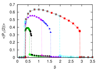
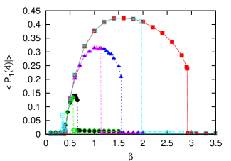
Figure 2: The measured vacuum expectation values for the open Wilson lines of length 2 and 4 lattice units, at $N=15,\,25,\,35$ (from left to right), and $\beta$ fixed by the Double Scaling condition. We observe symmetric phases at strong and at weak coupling, but at moderate coupling we discovered a phase of spontaneously broken translation symmetry. The weak coupling transition has a clear hysteresis behavior.

Fig. 3 shows the corresponding phase diagram. For any $N$ the strong coupling transition is at $\beta\approx 0.35$ (cf. Fig. 2), whereas the weak coupling transition occurs at a value of $\beta\propto N^{2}$. This means that the Double Scaling Limits — at fixed $\theta\propto Na^{2}\propto N/\beta^{2}$ — all lead to the broken phase, and not to the weak coupling phase as one might have expected. Hence it is the broken phase which is really relevant for the question if observables in NC $U(1)$ gauge theory are stable or not. The 1-loop result (13) refers to the weak coupling phase; it is therefore not relevant for the NC continuum limit (the Double Scaling Limit). In the broken phase we found stability for all observables that we measured NCQED .

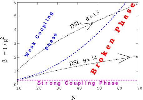
Figure 3: The phase diagram for pure $U(1)$ gauge theory in 4 dimensions, involving a (spatial) NC plane. At fixed size $N$, Poincaré symmetry is intact at strong and at weak coupling, but it is spontaneously broken in a moderate coupling phase. The Double Scaling Limits (DSL) — taken at fixed non-commutativity parameter $\theta$ — lead to the broken phase, which is therefore relevant for the NC continuum limit. In that phase, the (negative) IR singularity is not observed, and the system could be sensible.

This holds in particular for our explicit results for the dispersion relation of the NC photon. It was measured from the exponential decay of the Wilson line correlation function, separated in Euclidean time. We set the momentum components in the NC plane to zero, hence we measured the energy $E(p=p_{3})|_{p_{1}=p_{2}=0}\,$.

Fig. 4 (on the left) refers to the (symmetric) weak coupling phase. We see an energy dip at low momenta. This feature is fully consistent with the prediction (13) based on perturbation theory, which some people denote as “tachyonic behavior”. (Of course we cannot measure negative energies based on the decay of 2-point functions, but the feature observed here matches exactly such an IR instability).

However, as we pointed out above, the phase which really matters for a continuum limit to a NC space of infinite extent is the phase of broken Poincaré symmetry. The result in that phase is illustrated on the right-hand-side of Fig. 4. It follows the standard linear dispersion relation. Hence we do not see any non-commutativity effect for the dispersion in the commutative plane, but we do see that the disastrous negative IR divergence disappears. Our attempts to measure the dispersion relation also at finite momentum components in the NC plane were not successful, since we did not obtain an exponential decay of the Wilson line correlation functions.

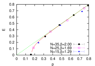
Figure 4: The dispersion relation of the NC photon in the symmetric weak coupling phase (on the left), and in the phase of broken Poincaré symmetry (on the right). We show the energy as a function of the commutative momentum component $p_{3}$, $E(p=p_{3})|_{p_{1}=p_{2}=0}\,$. Our result in the symmetric phase is consistent with the IR instability, which was predicted perturbatively LLT . (In contrast, a positive IR divergence has been observed in the NC $\lambda\phi^{4}$ model, where translation symmetry breaks as well NCphi4 .) The physically relevant result, however, is the dispersion in the broken phase, where the Double Scaling Limit ends up, and there we observe an IR stable behavior.

5 Conclusions

Lorentz Invariance Violation (LIV) has been searched for intensively in recent years, but so far it has not been observed anywhere. We reviewed a failed attempt which checked the photon dispersion relation based on Gamma Rays Bursts.

As one of the theoretical frameworks which could give rise to LIV we discussed quantum field theory — in particular pure $U(1)$ gauge theory — in a non-commutative space. Our non-perturbative study NCQED was based on Monte Carlo simulations in a space of Euclidean signature with one (spatial) non-commutative plane. The Double Scaling Limit extrapolates simultaneously to the continuum and to infinite volume at a fixed non-commutativity parameter. It leads to a phase of spontaneously broken Poincaré symmetry, which corresponds to a moderate coupling strength in finite volume.

In this limit we found evidence for convergent observables. This suggests that this model might be renormalizable, despite severe problems in its perturbative expansion LLT . In particular the photon dispersion in the Double Scaling Limit appears IR stable, though we could only measure it in the commutative plane. If one measures a deviation from the linear behavior in an NC direction, the confrontation with GRB data could establish a robust bound on $\|\Theta\|$ (the norm of the non-commutativity tensor) in Nature. So far we provided evidence that the photon may survive in a NC space, although perturbation theory found an negative IR divergence (that result only holds in the weak coupling phase, which turned out to be irrelevant for the NC continuum limit).

As an outlook on the phenomenological side, we mention that the Fermi Gamma-ray Space Telescope has been in orbit since June 2008. It monitors hundreds of GRBs per year, with sensitivity to photon energies $E\simeq 8~{}{\rm keV}\dots 300~{}{\rm GeV}$ Lamon . This could further boost the precision of Lorentz Invariance tests on cosmic photons Fermi , cf. Section 2.

Acknowledgment: I thank Jun Nishimura, Yoshiaki Susaki and Jan Volkholz for their collaboration in the work that I summarized here, and Frank Hofheinz for his assistance.

References

- (1) D. Mattingly, Living Rev. Rel. 8, 5 (2005). T. Jacobson, S. Liberati and D. Mattingly, Annals Phys. 321, 150–196 (2006). W. Bietenholz, arXiv:0806.3713 [hep-ph]; Fortschr. Phys. 57, 505–513 (2009). M. Galaverni and G. Sigl, Phys. Rev. D 78, 063003 (2008). S. Liberati and L. Maccione, Ann. Rev. Nucl. Part. Sci. 59, 245–267 (2009). L. Shao and B.-Q. Ma, arXiv:1007.2269 [hep-ph].
- (2) http://www.nasa.gov/missionpages/swift/bursts/farthestgrb.html
- (3) G. Amelino-Camelia et al., Nature 393, 763–765 (1998).
- (4) J.R. Ellis et al., Astropart. Phys. 25, 402–411 (2006); erratum, arXiv:0712.2781 [astro-ph].
- (5) V.A. Kostelecký and R. Lehnert, Phys. Rev. D 63, 065008 (2001).
- (6) S. Doplicher, K. Fredenhagen and J.E. Roberts, Commun. Math. Phys. 172, 187–220 (1995).
- (7) S. Minwalla, M. Van Raamsdonk and N. Seiberg, JHEP 02, 020 (2000).
- (8) R.J. Szabo, Phys. Rept. 378, 207–299 (2003).
- (9) A. González-Arroyo and M. Okawa, Phys. Rev. D 27, 2397–2411 (1983).
- (10) H. Aoki, N. Ishibashi, S. Iso, H. Kawai, Y. Kitazawa and T. Tada, Nucl. Phys. B 565, 176–192 (2000). J. Ambjørn, Y. Makeenko, J. Nishimura and R.J. Szabo, JHEP 05, 023 (2000).
- (11) N. Ishibashi, S. Iso, H. Kawai and Y. Kitazawa, Nucl. Phys. B 573, 573–593 (2000). D.J. Gross, A. Hashimoto and N. Itzhaki, Adv. Theor. Math. Phys. 4, 893–928 (2000).
- (12) A. Matusis, L. Susskind and N. Toumbas, JHEP 0012, 002 (2000).
- (13) G. Amelino-Camelia, L. Doplicher, S.-K. Nam and Y.-S. Seo, Phys. Rev. D 67, 085008 (2003).
- (14) F. Ruiz Ruiz, Phys. Lett. B 502, 274–278 (2001). K. Landsteiner, E. Lopez and M.H.G. Tytgat, JHEP 0106, 055 (2001). M. Van Raamsdonk, JHEP 0111, 006 (2001).
- (15) T. Mariz, J.R. Nascimento and V.O. Rivelles, Phys. Rev. D 75, 025020 (2007).
- (16) W. Bietenholz, J. Nishimura, Y. Susaki and J. Volkholz, JHEP 0610, 042 (2006).
- (17) K. Osterwalder and R. Schrader, Commun. Math. Phys. 31, 83–112 (1973).
- (18) W. Bietenholz, F. Hofheinz and J. Nishimura, JHEP 0209, 009 (2002).
- (19) W. Bietenholz, A. Bigarini and A. Torrielli, JHEP 0708, 041 (2007).
- (20) W. Bietenholz, F. Hofheinz and J. Nishimura, JHEP 0406, 042 (2004).
- (21) R. Lamon, JCAP 0808, 022 (2008) 022.
- (22) Fermi GBM/LAT Collaborations (A.A. Abdo et al.), Nature 462, 331–334 (2009). L. Shao, Z. Xiao and B.-Q. Ma, Astropart. Phys. 33, 312–315 (2010).