INSTITUT NATIONAL DE RECHERCHE EN INFORMATIQUE ET EN AUTOMATIQUE

Monte Carlo Methods for Top-k Personalized PageRank Lists and Name Disambiguation
Konstantin Avrachenkov — Nelly Litvak — Danil Nemirovsky — Elena Smirnova — Marina Sokol N° 7367
August 2010

Abstract: We study a problem of quick detection of top-k Personalized PageRank lists. This problem has a number of important applications such as finding local cuts in large graphs, estimation of similarity distance and name disambiguation. In particular, we apply our results to construct efficient algorithms for the person name disambiguation problem. We argue that when finding top-k Personalized PageRank lists two observations are important. Firstly, it is crucial that we detect fast the top-k most important neighbours of a node, while the exact order in the top-k list as well as the exact values of PageRank are by far not so crucial. Secondly, a little number of wrong elements in top-k lists do not really degrade the quality of top-k lists, but it can lead to significant computational saving. Based on these two key observations we propose Monte Carlo methods for fast detection of top-k Personalized PageRank lists. We provide performance evaluation of the proposed methods and supply stopping criteria. Then, we apply the methods to the person name disambiguation problem. The developed algorithm for the person name disambiguation problem has achieved the second place in the WePS 2010 competition.

Key-words: Personalized PageRank, Monte Carlo Methods, Person Name Disambiguation

Les Méthodes Monte Carlo pour Top-k Listes de PageRank Personnalisé avec l’application a disambiguation de noms

Résumé : Nous étudions le problème de détection rapide de top-k listes de PageRank Personnalisé. Ce problème a plusieurs applications importantes telles que la recherche des coupes locales de graphes, l’éstimation de la distance de la similarité, et disambiguation de noms. En particulier, nous appliquons nos resultats a construction des algorithmes efficaces pour le problème de disambiguation de noms de personnes. Notre étude est basé sur les deux observations suivantes. D’abord, il est cruciale que nous trouvons rapidement les top-k voisins les plus importants d’un noeud. Cependant, l’ordre exact dans le top-K ainsi que les valeurs exactes de PageRank sont de loin pas si cruciale. Deuxiemement, un petit nombre de elements erronés dans les top-k listes ne degrade pas vraiment la qualite des listes de top-k, mais ce sacrifice améliore significativement la performance des algorithmes. Sur la base de ces deux observations clés nous proposons des méthodes de type Monte Carlo pour la détection rapide de top-k listes de PageRank Personnalisé. Nous offrons l’évaluation des performances des méthodes proposées et nous donnons critères d’arrêt. En suite, nous appliquons les méthodes au problème de disambiguation de noms de personnes. Notre approche basé sur PageRank Personnalisé et les méthodes Monte Carlo a recu le deuxième prix de la compétion WePS 2010.

Mots-clés : PageRank Personnalisé, Méthodes Monte Carlo, Disambiguation de Noms de Personnes

1 Introduction

Personalized PageRank or Topic-Sensitive PageRank [18] is a generalization of PageRank [10]. Personalized PageRank is a stationary distribution of a random walk on an entity graph. With some probability the random walk follows an outgoing link with uniform distribution and with the complementary probability the random walk jumps to a random node according to a personalization distribution. Personalized PageRank has a number of applications. Let us name just a few. In the original paper [18] Personalized PageRank was used to introduce the personalization in the Web search. In [11, 25, 31] Personalized PageRank was suggested for finding related entities. In [28] Green measure, which is closely related to Personalized PageRank, was suggested for finding related pages in Wikipedia. In [2, 3] Personalized PageRank was used for finding local cuts in graphs and in [6] the Personalized PageRank was applied for clustering large hyper-text document collections. In many applications we are interested in detecting top-k elements with the largest values of Personalized PageRank. Our present work on detecting top-k elements is driven by the following two key observations:

Observation 1: Often it is crucial that we detect fast the top-k elements with the largest values of the Personalized PageRank, while the exact order in the top-k list as well as the exact values of the Personalized PageRank are by far not so important.

Observation 2: It is not crucial that the top-k list is determined exactly, and therefore we may apply a relaxation that allows a small number of elements to be placed erroneously in the top-k list. If the Personalized PageRank values of these elements are of a similar order of magnitude as in the top-k list, then such relaxation does not affect applications, but it enables us to take advantage of the generic “80/20 rule”: 80% of the result is achieved with 20% of efforts.

We argue that the Monte Carlo approach naturally takes into account the two key observations. In [9] the Monte Carlo approach was proposed for the computation of the standard PageRank. The estimation of the convergence rate in [9] was very pessimistic. Then, the implementation of the Monte Carlo approach was improved in [14] and also applied there to Personalized PageRank. Both [9] and [14] only use end points as information extracted from the random walk. Moreover, the approach of [14] requires extensive precomputation efforts and is very demanding in storage resource. In [5], it has been shown that to find elements with large values of PageRank the Monte Carlo approach requires about the same number of operations as one iteration of the power iteration method. In the present work we show that to detect top-k list of elements when $k$ is not large we need even smaller number of operations. In our test on the Wikipedia entity graph with about 2 million nodes we have observed that typically few thousands of operations are enough to detect the top-10 list with just two or three erroneous elements. Namely to detect a relaxation of the top-10 list we spend just about 1-5% of operations required by one power iteration. In the present work we provide theoretical justification for such a small amount of required operations. We also apply the Monte Carlo methods for Personalized PageRank to the person name disambiguation problem. Name resolution problem consists in clustering search results for a person name according to found namesakes. We found that considering patterns of Web structure for name resolution problem results in methods with very competitive performance.

2 Monte Carlo methods

Given a directed or undirected graph connecting some entities, the Personalized PageRank $\pi(s,c)$ with a seed node $s$ and a damping parameter $c$ is defined as a solution of the following equations

$$\pi(s,c)=c\pi(s,c)P+(1-c){\bf 1}_{s}^{T},$$

$$\sum_{j=1}^{n}\pi_{j}(s,c)=1.$$

where ${\bf 1}_{s}^{T}$ is a row unit vector with one in the $s^{\mathrm{th}}$ entry and all the other elements equal to zero, $P$ is the transition matrix associated with the entity graph and $n$ is the number of entities. Equivalently, the Personalized PageRank can be given by the explicit formula [24, 26]

$$\pi(s,c)=(1-c){\bf 1}_{s}^{T}[I-cP]^{-1}.$$ (1)

Whenever the values of $s$ and $c$ are clear from the context we shall simply write $\pi$.

We would like to note that often the Personalized PageRank is defined with a general distribution $v$ in place of ${\bf 1}_{s}^{T}$. However, typically distribution $v$ has a small support. Then, due to linearity, the problem of Personalized PageRank with distribution $v$ reduces to the problem of Personalized PageRank with distribution ${\bf 1}_{s}^{T}$ [19].

In this work we consider two Monte Carlo algorithms. The first algorithm is inspired by the following observation. Consider a random walk $\{X_{t}\}_{t\geq 0}$ that starts from node $s$, i.e, $X_{0}=s$. Let at each step the random walk terminate with probability $1-c$ and make a transition according to the matrix $P$ with probability $c$. Then, the end-points of such a random walk has the distribution $\pi(s,c)$.

Algorithm 2.1 (MC End Point)

Simulate $m$ runs of the random walk $\{X_{t}\}_{t\geq 0}$ initiated at node $s$. Evaluate $\pi_{j}$ as a fraction of $m$ random walks which end at node $j\in 1,\dots,n$.

The next observation leads to another Monte Carlo algorithm for Personalized PageRank. Denote $Z:=[I-cP]^{-1}$. We have the following interpretation for the elements of matrix $Z$: $z_{sj}=E_{s}[N_{j}]$, where $N_{j}$ is the number of visits to node $j$ by a random walk before a restart, and $E_{s}[\cdot]$ is the expectation assuming that the random walk started at node $s$. Namely, $z_{sj}$ is the expected number of visits to node $j$ by the random walk initiated at state $s$ with the run time geometrically distributed with parameter $c$. Thus, the formula (1) suggests the following estimator for Personalized PageRank

$$\hat{\pi}_{j}(s,c)=(1-c)\frac{1}{m}\sum_{r=1}^{m}N_{j}(s,r),$$ (2)

where $N_{j}(s,r)$ is the number of visits to state $j$ during the run $r$ of the random walk initiated at node $s$. Thus, we can suggest the second Monte Carlo algorithm.

Algorithm 2.2 (MC Complete Path)

Simulate $m$  runs of the random walk $\{X_{t}\}_{t\geq 0}$ initiated at node $s$. Evaluate $\pi_{j}$ as the total number of visits to node $j$ multiplied by $(1-c)/m$.

As outputs of the proposed algorithms we would like to obtain with high probability either a top-k list of nodes or a top-k basket of nodes.

Definition 2.1

The top-$k$ list of nodes is a list of $k$ nodes with largest Personalized PageRank values arranged in a descending order of their Personalized PageRank values.

Definition 2.2

The top-$k$ basket of nodes is a set of $k$ nodes with largest Personalized PageRank values with no ordering required.

It turns out that it is beneficial to relax our goal and to obtain a top-$k$ basket with a small number of erroneous elements.

Definition 2.3

We call relaxation-$l$ top-$k$ basket a realization when we allow at most $l$ erroneous elements from top-$k$ basket.

In the present work we aim to estimate the numbers of random walk runs $m$ sufficient for obtaining top-$k$ list or top-$k$ basket or relaxation-$l$ top-$k$ basket with high probability. In particular, we demonstrate that ranking converges considerably faster than the values of Personalized PageRank and that a relaxation-$l$ with quite small $l$ helps significantly.

Let us begin the analysis of the algorithms with the help of an illustrating example on the Wikipedia entity graph. We shall carry out the development of the example throughout the paper. There is a number of reasons why we have chosen the Wikipedia entity graph. Firstly, the Wikipedia entity graph is a non-trivial example of a complex network. Secondly, it has been shown that the Green’s measure which is closely related to Personalized PageRank is a good measure of similarity on the Wikipedia entity graph [28]. In addition, we note that Personalized PageRank is a good similarity measure also in social networks [25] and on the Web [29]. Thirdly, we apply our person name disambiguation algorithm on the real Web for which we cannot compute the real values of the Personalized PageRank. The Personalized PageRank can be computed with high precision for the Wikipedia entity graph with the help of BVGraph/WebGraph framework [7].

Illustrating example: Since our work is concerned with application of Personalized PageRank to the name disambiguation problem, let us choose a common name. One of the most common English names is Jackson. We have selected three Jacksons who have entries in Wikipedia: Jim Jackson (ice hockey), Jim Jackson (sportscaster) and Michael Jackson. Two Jacksons have even a common given name and both worked in ice hockey, one as an ice hockey player and another as an ice hockey sportscaster. In Tables 1-3 we provide the exact lists of top-10 Wikipedia articles arranged according to Personalized PageRank vectors. In Table 1 the seed node for the Personalized PageRank is the article Jim Jackson (ice hockey), in Table 2 the seed node is the article Jim Jackson (sportscaster), and in Table 3 the seed node is the article Michael Jackson. We observe that each top-10 list identifies quite well its seed node. This gives us hope that Personalized PageRank can be useful in the name disambiguation problem. (We shall discuss more the name disambiguation problem in Section 6.) Next we run the Monte Carlo End Point method starting from each seed node. We note that top-10 lists obtained by Monte Carlo methods also identify well the original seed nodes. It is interesting to note that to obtain a relaxed top-10 list with two or three erroneous elements we need different number of runs for different seed nodes. To obtain a good relaxed top-10 list for Michael Jackson we need to perform about 50000 runs, whereas for a good relaxed top-10 list for Jim Jackson (ice hockey) we need to make just 500 runs. Intuitively, the more immediate neighbours a node has, the larger number of Monte Carlo steps is required. Starting from a node with many immediate neighbours the Monte Carlo method easily drifts away. In Figures 1-3 we present examples of typical runs of the Monte Carlo End Point method for the three different seed nodes. An example of the Monte Carlo Complete Path method for the seed node Michael Jackson is given in Figure 4. Indeed, as expected, it outperforms the Monte Carlo End Point method. In the following sections we shall quantify all the above qualitative observations.

Table 1: Top-10 lists for Jim Jackson (ice hockey)

No.	Exact Top-10 List	MC End Point (m=500)
1	Jim Jackson (ice hockey)	Jim Jackson (ice hockey)
2	Ice hockey	Winger (ice hockey)
3	National Hockey League	1960
4	Buffalo Sabres	National Hockey League
5	Winger (ice hockey)	Ice hockey
6	Calgary Flames	February 1
7	Oshawa	Buffalo Sabres
8	February 1	Oshawa
9	1960	Calgary Flames
10	Ice hockey rink	Columbus Blue Jackets

Table 2: Top-10 lists for Jim Jackson (sportscaster)

No.	Exact Top-10 List	MC End Point (m=5000)
1	Jim Jackson (sportscaster)	Jim Jackson (sportscaster)
2	Philadelphia Flyers	Steve Coates
3	United States	New York
4	Philadelphia Phillies	United states
5	Sportscaster	Philadelphia Flyers
6	Eastern League (baseball)	Gene Hart
7	New Jersey Devils	Sportscaster
8	New York - Penn League	New Jersey Devils
9	Play-by-play	Mike Emrick
10	New York	New York - Penn League

Table 3: Top-10 lists for Michael Jackson

No.	Exact Top-10 List	MC End Point (m=50000)
1	Michael Jackson	Michel Jackson
2	United States	United states
3	Billboard Hot 100	Pop music
4	The Jackson 5	Epic Records
5	Pop music	Billboard Hot 100
6	Epic records	Motown Records
7	Motown Records	The Jackson 5
8	Soul music	Singing
9	Billboard (magazine)	Hip Hop music
10	Singing	Gary, Indiana

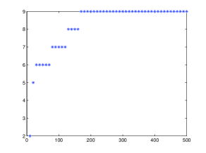
Figure 1: The number of correctly detected elements by MC End Point for the seed node Jim Jackson (ice hockey).

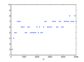
Figure 2: The number of correctly detected elements by MC End Point for the seed node Jim Jackson (sportscaster).

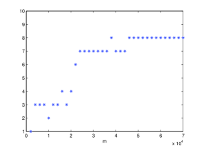
Figure 3: The number of correctly detected elements by MC End Point for the seed node Michael Jackson.

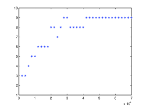
Figure 4: The number of correctly detected elements by MC Complete Path for the seed node Michael Jackson.

3 Variance based performance comparison and CLT approximations

In the MC End Point algorithm the distribution of end points is multinomial [20]. Namely, if we denote by $L_{j}$ the number of paths that end at node $j$ after $m$ runs, then we have

$$P\{L_{1}=l_{1},L_{2}=l_{2},\dots,L_{n}=l_{n}\}=\frac{m!}{l_{1}!l_{2}!\cdots l_{n}!}\pi_{1}^{l_{1}}\pi_{2}^{l_{2}}\cdots\pi_{n}^{l_{n}}.$$ (3)

Thus, the standard deviation of the MC End Point estimator for the $k^{\mathrm{th}}$ element is given by

$$\sigma(\hat{\pi}_{k})=\sigma(L_{k}/m)=\frac{1}{\sqrt{m}}\sqrt{\pi_{k}(1-\pi_{k})}.$$ (4)

An expression for the standard deviation of the MC Complete Path is more complicated. From (2), it follows that

$$\sigma(\hat{\pi}_{k})=\frac{(1-c)}{\sqrt{m}}\sigma(N_{k})=\frac{(1-c)}{\sqrt{m}}\sqrt{E_{s}\{N_{k}^{2}\}-E_{i}\{N_{k}\}^{2}}.$$ (5)

First, we recall that

$$E_{s}\{N_{k}\}=z_{sk}=\pi_{k}(s)/(1-c).$$ (6)

Then, from [21], it is known that the second moment of $N_{k}$ is given by

$$E_{s}\{N_{k}^{2}\}=[Z(2Z_{dg}-I)]_{sk},$$

where $Z_{dg}$ is a diagonal matrix having as its diagonal the diagonal of matrix $Z$ and $[A]_{ik}$ denotes the $(i,k)^{\mathrm{th}}$ element of matrix $A$. Thus, we can write

$$E_{s}\{N_{k}^{2}\}={\bf 1}_{s}^{T}Z(2Z_{dg}-I){\bf 1}_{k}=\frac{1}{1-c}\pi(s)(2Z_{dg}-I){\bf 1}_{k}$$

$$=\frac{1}{1-c}\left(\frac{1}{1-c}\pi_{k}(s)\pi_{k}(k)-\pi_{k}(s)\right).$$ (7)

Substituting (6) and (7) into (5), we obtain

$$\sigma(\hat{\pi}_{k})=\frac{1}{\sqrt{m}}\sqrt{\pi_{k}(s)(2\pi_{k}(k)-(1-c)-\pi_{k}(s))}.$$ (8)

Since $\pi_{k}(k)\approx 1-c$, we can approximate $\sigma(\hat{\pi}_{k})$ with

$$\sigma(\hat{\pi}_{k})\approx\frac{1}{\sqrt{m}}\sqrt{\pi_{k}(s)((1-c)-\pi_{k}(s))}.$$

Comparing the latter expression with (4), we can see that MC End Point requires approximately $1/(1-c)$ steps more than MC Complete Path. This was expected as MC End Point uses only information from end points of the random walks. We would like to emphasize that $1/(1-c)$ can be a significant coefficient. For instance, if $c=0.85$, then $1/(1-c)\approx 6.7$.

Let us provide central limit type theorems for our estimators.

Theorem 3.1

For large $m$, a multivariate normal density approximation to the multinomial distribution $(\ref{chap:top-k:multinom})$ is given by

$$f(l_{1},l_{2},\dots,l_{n})=\left(\frac{1}{2\pi m}\right)^{(n-1)/2}\times$$

$$\left(\frac{1}{n\pi_{1}\pi_{2}\cdots\pi_{n}}\right)^{1/2}\exp\left\{-\frac{1}{2}\sum_{i=1}^{n}\frac{(l_{i}-m\pi_{i})^{2}}{m\pi_{i}}\right\},$$ (9)

subject to $\sum_{i=1}^{n}l_{i}=m$.

Proof. See [23] and [30].

$\Box$

Now we consider MC Complete Path. First, we note that the vectors $N(s,r)=(N_{1}(s,r),\dots,N_{n}(s,r))$ with $r=1,2,\dots$ form a sequence of i.i.d. random vectors. Hence, we can apply the multivariate central limit theorem. Denote

$$\hat{N}(s,m)=\frac{1}{m}\sum_{r=1}^{m}N(s,r).$$ (10)

Theorem 3.2

Let $m$ go to infinity. Then, we have the following convergence in distribution to a multivariate normal distribution

$$\sqrt{m}\left(\hat{N}(s,m)-\bar{N}\right)\stackrel{{\scriptstyle D}}{{\longrightarrow}}{\cal N}(0,\Sigma(s)),$$

where $\bar{N}(s)={\bf 1}^{T}_{s}Z$ and $\Sigma(s)=E\{N^{T}(s,r)N(s,r)\}-\bar{N}^{T}(s)\bar{N}(s)$ is a covariance matrix, which can be expressed as

$$\Sigma(s)=\Omega\left(s\right)Z+Z^{T}\Omega\left(s\right)-\Omega\left(s\right)-Z^{T}{\bf 1}_{s}{\bf 1}^{T}_{s}Z.$$ (11)

where the matrix $\Omega(s)=\left\{\omega_{jk}(s)\right\}$ is defined by

$$\omega_{jk}(s)=\left\{\begin{array}[]{ll}z_{sj},&\mbox{if $j=k$},\\ 0,&\mbox{otherwise}.\end{array}\right.$$

Proof. The convergence follows from the standard multivariate central limit theorem. We only need to establish the formula for the covariance matrix.

The covariance matrix can be expressed as follows [27]:

$$\Sigma(s)=\sum_{j=1}^{n}z_{sj}\left(D(j)Z+ZD(j)-D(j)\right)-Z^{T}{\bf 1}_{s}{\bf 1}^{T}_{s}Z,$$ (13)

where $D(j)$ is defined by

$$d_{kl}(j)=\left\{\begin{array}[]{ll}1,&\mbox{if $k=l=j$},\\ 0,&\mbox{otherwise}.\end{array}\right.$$

Let us consider $\sum_{j=1}^{n}z_{sj}D(j)Z$ in component form.

$$\sum_{j=1}^{n}z_{sj}\sum_{\varphi=1}^{n}d_{l\varphi}(j)z_{\varphi k}=\sum_{j=1}^{n}z_{sj}\delta_{lj}z_{jk}=z_{sl}z_{lk}=\sum_{j=1}^{n}\omega_{lj}(s)z_{jk},$$

and it implies that $\sum_{j=1}^{n}z_{sj}D(j)Z=\Omega(s)Z$. Symmetrically, $\sum_{j=1}^{n}z_{sj}ZD(j)=Z^{T}\Omega(s)$. Equality $\sum_{j=1}^{n}z_{sj}D(j)=\Omega(s)$ can be easily established. This completes the proof.

$\Box$

We would like to note that in both cases we obtain the convergence to rank deficient (singular) multivariate normal distributions.

Of course, one can use the joint confidence intervals for the CLT approximations to estimate the quality of top-$k$ list or basket. However, it appears that we can propose more efficient methods. Let us consider as an example mutual ranking of two elements $k$ and $l$ from a list. For illustration purpose, assume that the elements are independent and have the same variance. Suppose that we apply some version of CLT approximation. Then, we need to compare two normal random variables $Y_{k}$ and $Y_{l}$ with means $\pi_{k}$ and $\pi_{l}$, and with the same variance $\sigma^{2}$. Without loss of generality we assume that $\pi_{k}>\pi_{l}$. Then, it can be shown that one needs twice as more experiments to guarantee that the random variable $Y_{k}$ and $Y_{l}$ inside their confidence intervals with the confidence level $\alpha$ than to guarantee that $P\{Y_{k}\geq Y_{l}\}=\alpha$. Thus, it is more beneficial to look at the order of elements rather than their absolute values. We shall pursue this idea in more detail in the ensuing sections.

4 Convergence based on order

For the two introduced Monte Carlo methods we would like to calculate or to estimate a probability that after a given number of steps we correctly obtain top-$k$ list or top-$k$ basket. Namely, we need to calculate the probabilities $P\{L_{1}>\dots>L_{k}>L_{j},\forall j>k\}$ and $P\{L_{i}>L_{j},\forall i,j:i\leq k<j\}$ respectively, where $L_{k}$, $k\in 1,\dots,n$, can be either the Monte Carlo estimates of the ranked elements or their CLT approximations. We refer to these probabilities as the ranking probabilities and we refer to complementary probabilities as misranking probabilities [8]. Even though, these probabilities are easy to define, it turns out that because of combinatorial explosion their exact calculation is infeasible for non-trivial cases.

We first propose to estimate the ranking probabilities of top-$k$ list and top-$k$ basket with the help of Bonferroni inequality [15]. This approach works for reasonably large values of $m$.

4.1 Estimation by Bonferroni inequality

Drawing correctly the top-$k$ basket is defined by the event

$$\bigcap_{i\leq k<j}\{L_{i}>L_{j}\}.$$

Let us apply to this event the Bonferroni inequality

$$P\left\{\bigcap_{s}A_{s}\right\}\geq 1-\sum_{s}P\left\{\bar{A}_{s}\right\}.$$

We obtain

$$P\left\{\bigcap_{i\leq k<j}\{L_{i}>L_{j}\}\right\}\geq 1-\sum_{i\leq k<j}P\left\{\overline{\{L_{i}>L_{j}\}}\right\}.$$

Equivalently, we can write the following upper bound for the misranking probability

$$1-P\left\{\bigcap_{i\leq k<j}\{L_{i}>L_{j}\}\right\}\leq\sum_{i\leq k<j}P\left\{L_{i}\leq L_{j}\right\}.$$ (14)

We note that it is very good that we obtain an upper bound in the above expression for the misranking probability, since the upper bound will provide a guarantee on the performance of our algorithms. Since in the MC End Point method the distribution of end points is multinomial (see (3)), the probability $P\left\{L_{i}\leq L_{j}\right\}$ is given by

$$P\{L_{i}\leq L_{j}\}=$$ (15)

$$\sum_{l_{i}+l_{j}\leq m,\ l_{i}\leq l_{j}}\frac{m!}{l_{i}!l_{j}!(m-l_{i}-l_{j})!}\pi_{i}^{l_{i}}\pi_{j}^{l_{j}}(1-\pi_{i}-\pi_{j})^{m-l_{i}-l_{j}}.$$

The above formula can only be used for small values of $m$. For large values of $m$, we can use the CLT approximation for the both MC methods. To distinguish between the original number of hits and its CLT approximation, we use $L_{j}$ for the original number of hits at node $j$ and $Y_{j}$ for its CLT approximation. First, we obtain a CLT based expression for the misranking probability for two nodes $P\left\{Y_{i}\leq Y_{j}\right\}$. Since the event $\left\{Y_{i}\leq Y_{j}\right\}$ coincides with the event $\left\{Y_{i}-Y_{j}\leq 0\right\}$ and a difference of two normal random variables is again a normal random variable, we obtain

$$P\left\{Y_{i}\leq Y_{j}\right\}=P\left\{Y_{i}-Y_{j}\leq 0\right\}=1-\Phi(\sqrt{m}\rho_{ij}),$$

where $\Phi(\cdot)$ is the cumulative distribution function for the standard normal random variable and

$$\rho_{ij}=\frac{E[Y_{i}]-E[Y_{j}]}{\sqrt{\sigma^{2}(Y_{i})-2\mbox{cov}(Y_{i},Y_{j})+\sigma^{2}(Y_{j})}}.$$

For large $m$, the above expression can be bounded by

$$P\left\{Y_{i}\leq Y_{j}\right\}\leq\frac{1}{\sqrt{2\pi}}e^{-\frac{\rho_{ij}^{2}}{2}m}$$

Since the misranking probability for two nodes $P\left\{Y_{i}\leq Y_{j}\right\}$ decreases when $j$ increases, we can write

$$1-P\left\{\bigcap_{i\leq k<j}\{Y_{i}>Y_{j}\}\right\}\leq$$

$$\sum_{i=1}^{k}\left(\sum_{j=k+1}^{j^{*}}P\left\{Y_{i}\leq Y_{j}\right\}+\sum_{j=j^{*}+1}^{n}P\left\{Y_{i}\leq Y_{j^{*}}\right\}\right),$$

for some $j^{*}$. This gives the following upper bound

$$1-P\left\{\bigcap_{i\leq k<j}\{Y_{i}>Y_{j}\}\right\}\leq$$

$$\sum_{i=1}^{k}\sum_{j=k+1}^{j^{*}}(1-\Phi(\sqrt{m}\rho_{ij}))+\frac{n-j^{*}}{\sqrt{2\pi}}\sum_{i=1}^{k}e^{-\frac{\rho_{ij^{*}}^{2}}{2}m}.$$ (16)

Since we have a finite number of terms in the right hand side of expression (16), we conclude that

Theorem 4.1

The misranking probability of the top-$k$ basket tends to zero with geometric rate, that is,

$$1-P\left\{\bigcap_{i\leq k<j}\{Y_{i}>Y_{j}\}\right\}\leq Ca^{m},$$

for some $C>0$ and $a\in(0,1)$.

We note that $\rho_{ij}$ has a simple expression in the case of the multinomial distribution

$$\rho_{ij}=\frac{\pi_{i}-\pi_{j}}{\sqrt{\pi_{i}(1-\pi_{i})+2\pi_{i}\pi_{j}+\pi_{j}(1-\pi_{j})}}.$$

For MC Complete Path $\sigma^{2}(Y_{i})=\Sigma_{ii}(s)$ and $\mbox{cov}(Y_{i},Y_{j})=\Sigma_{ij}(s)$ where $\Sigma_{ii}(s)$ and $\Sigma_{ij}(s)$ can be calculated by (11).

The Bonferroni inequality for the top-$k$ list gives

$$P\{Y_{1}>\dots>Y_{k}>Y_{j},\forall j>k\}\geq$$

$$1-\sum_{1\leq i\leq k-1}P\{Y_{i}\leq Y_{i+1}\}-\sum_{k+1\leq j\leq n}P\{Y_{k}\leq Y_{j}\}.$$

Using misranking probability for two elements, one can obtain more informative bounds for the top-$k$ list as was done above for the case of top-$k$ basket. For the misranking probability of the top-$k$ list we also have a geometric rate of convergence.

Illustrating example (cont.): In Figure 5 we plot Bonferroni bound for the misranking probability given by (14) with the CLT approximation for the pairwise misranking probability. We note that the Bonferroni inequality provides quite conservative estimation for the necessary number of MC runs. Below we shall try to obtain a better estimation.

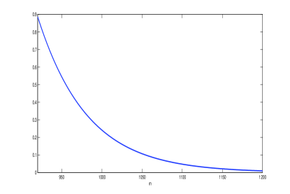
Figure 5: Bonferroni bound for MC End Point for the seed node Jim Jackson (ice hockey) and top-9 basket.

4.2 Approximation based on order statistics

We can obtain more insight on the convergence based on order with the help of order statistics [13].

Let us denote by $X_{t}\in\{1,...,n\}$ the node hit by the random walk $t$, and let $X$ have the same distribution as $X_{t}$. Now let us consider the $s$-th order statistic of the random variables $X_{t}$, $t=1,...,m$. We can calculate its cumulative distribution function as follows:

$$P\{X_{(s)}\leq k\}=\sum_{j=0}^{m-s}{m\choose j}P\{X>k\}^{j}P\{X\leq k\}^{m-j}$$

$$=1-\sum_{i=0}^{s-1}{m\choose i}P\{X\leq k\}^{i}(1-P\{X\leq k\})^{m-i}$$ (17)

It is interesting to observe that $P\{X_{(s)}\leq k\}$ depends on the Personalized PageRank distribution only via $P\{X\leq k\}=\pi_{1}+...+\pi_{k}$ showing insensitivity property with respect to the distribution’s tail.

Next we notice that a reasonable minimal value of $m$ corresponds to the case when the elements of the top-$k$ basket obtain $r$ or more hits with a high probability and the other elements outside the top-$k$ basket will have very small probability of $r$-times hit. Thus, the probability $P\{X_{(rk)}\leq k\}$ should be reasonably high and the probability of hitting $r$ times the elements outside the top-$k$ basket should be small. The probability to hit the element $j$ at least $r$ times is given by

$$P\{Y_{j}\geq r\}=1-\sum_{\nu=0}^{r-1}{{m}\choose{\nu}}\pi_{j}^{\nu}(1-\pi_{j})^{m-\nu}.$$ (18)

Hence, choosing $m$ for the fast detection of the top-$k$ basket we need to satisfy two criteria: (i) $P\{X_{(rk)}\leq k\}\geq 1-\varepsilon_{1}$, and (ii) $P(Y_{j}\geq r)\leq\varepsilon_{2}$ for $j>k$. The probability in (i) and $P(Y_{j}\geq r)$ in (ii) are both increasing with $m$. However, we have observed (see the illustrating example next) that for a given $m$ the probabilities given in (17) and (18) drop drastically with $r$. Thus, we hope to be able to find a proper balance between $m$ and $r$ for a reasonably small value of $r$.

We can further improve the computational efficiency for order statistics distribution (17) with the help of incomplete Beta function as suggested in [1]. Namely, in our case we have

$$P\{X_{(s)}\leq k\}=I_{P\{X\leq k\}}(s,m-s+1),$$ (19)

where

$$I_{x}(a,b)=\frac{1}{B(a,b)}\int_{0}^{x}y^{a-1}(1-y)^{b-1}dy$$

is the incomplete Beta function.

Illustrating example (cont.): We first consider the seed node Jim Jackson (ice hochey). In Figure 6 we plot the probabilities given by (17) and (18) for $m\leq 2000$, $r=5$, and $k=9$. For instance, if we take $m=250$, $P\{X_{(45)}\leq 9\}=0.9999$ and $P\{Y_{10}\geq 5\}=4.29\times 10^{-5}$. Thus, with very high probability we collect 45 hits inside the top-9 basket and the probability for the 10-th element to receive more than or equal to 5 hits is very small. Figure 1 confirms that taking $m=250$ is largely enough to detect the top-9 basket. Suppose now that we want to detect the top-10 basket. Then, Figure 7 corresponding to $m\leq 10000$ , $r=18$ and $k=10$ suggests that to obtain correctly top-10 basket with high probability we need to spend about four times more operations than for the case of the top-9 basket. Here we already see an illustration to the “80/20 rule” which we discuss more in the next section. Now let us consider the seed node Michael Jackson. In Figure 8 we plot the probabilities given by (17) and (18) for $m\leq 100000$, $r=57$, $k=10$ and $j=11$. We have $P\{X_{(570)}\leq 10\}=0.9717$ and $P\{Y_{11}\geq 57\}=0.2338$. Even though there is a significant chance to get some erroneous elements in the top-10 list, as Figure 9 suggests we get “high quality” erroneous elements. Specifically, we have $P\{Y_{100}\geq 57\}=0.0077$ and $P\{Y_{500}\geq 57\}=8.8\times 10^{-47}$.

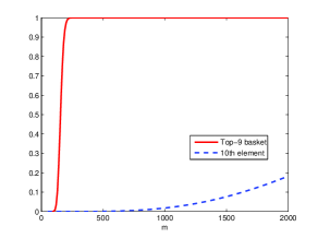
Figure 6: Evaluations based on order statistics for the seed node Jim Jackson (ice hockey): $P\{X_{(rk)}\leq k\}$ (solid line) and $P\{L_{j}\geq r\}$ (dash line), $k=9$, $j=10$, $r=5$.

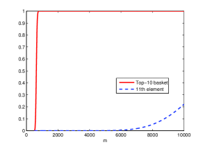
Figure 7: Evaluations based on order statistics for the seed node Jim Jackson (ice hockey): $P\{X_{(rk)}\leq k\}$ (solid line) and $P\{L_{j}\geq r\}$ (dash line), $k=10$, $j=11$, $r=18$.

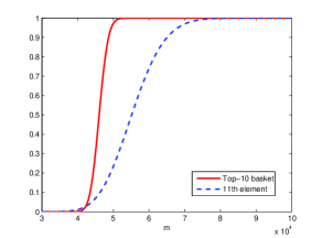
Figure 8: Evaluations based on order statistics for the seed node Michael Jackson: $P\{X_{(rk)}\leq k\}$ (solid line) and $P\{L_{j}\geq r\}$ (dash line), $k=10$, $j=11$, $r=57$.

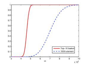
Figure 9: Evaluations based on order statistics for the seed node Michael Jackson: $P\{X_{(rk)}\leq k\}$ (solid line) and $P\{L_{j}\geq r\}$ (dash line), $k=10$, $j=100$, $r=57$.

5 Solution relaxation

In this section we analytically evaluate the average number of correctly identified top-$k$ nodes. We use the relaxation by allowing this number to be smaller than $k$. Our goal is to provide a mathematical evidence for the observed “80/20 behavior” of the algorithm: 80 percent of the top-$k$ nodes are identified correctly in a very short time. Accordingly, we evaluate the number of experiments $m$ for obtaining high quality top-$k$ lists.

Let $M_{0}$ be a number of correctly identified elements in the top-$k$ basket. In addition, denote by $K_{i}$ the number of nodes ranked not lower than $i$. Formally,

$$K_{i}=\sum_{j\neq i}1\{L_{j}\geq L_{i}\},\quad i=1,\ldots,k.$$

Clearly, placing node $i$ in the top-$k$ basket is equivalent to the event $[K_{i}<k]$, and thus we obtain

$$E(M_{0}) =E\left(\sum_{i=1}^{k}1\{\mbox{$K_{i}<k$}\}\right)=\sum_{i=1}^{k}P(\mbox{$K_{i}<k$}).$$ (20)

To evaluate $E(M_{0})$ by (20) we need to compute the probabilities $P(K_{i}<k)$ for $i=1,\ldots,k$. Direct evaluation of these probabilities is computationally intractable. A Markov chain approach based on the representations from [12] is more efficient, but this method, too, resulted in extremely demanding numerical schemes in realistic scenarios. Thus, to characterize the algorithm performance, we suggest to use two simplification steps: approximation and Poissonisation.

Poissonisation is a common technique for analyzing occupancy measures [16]. Clearly, the End Point algorithm is nothing else but an occupancy scheme where each independent experiment (random walk) results in placing one ball (visit) to an urn (node of the graph). Under Poissonisation, we assume that the number of random walks is not a fixed value $m$ but a Poisson random variable $M$ with mean $m$. In this scenario, the number $Y_{j}$ of visits to page $j$ has a Poisson distribution with parameter $m\pi_{j}$ and is independent of $Y_{i}$ for $i\neq j$. Because the number of hits in the Poissonised model is different from the number of original hits, we use the notation $Y_{i}$ instead of $L_{j}$. Poissonisation simplifies the analysis considerably due to the imposed independence of the $Y_{j}$’s.

Next to Poissonisation, we also apply approximation of $M_{0}$ by a closely related measure $M_{1}$:

$$M_{1}:=k-\sum_{i=1}^{k}(K^{\prime}_{i}/{k}),$$

where $K^{\prime}_{i}$ denotes the number of pages outside the top-$k$ that are ranked higher than node $i=1,\ldots,k$. The idea behind $M_{1}$ is as follows: $K_{i}^{\prime}$ is the number of mistakes with respect to node $i$ that lead to errors in the identified top-$k$ list. The sum in the definition of $M_{1}$ is the average number of such mistakes with respect to each of the top-$k$ nodes.

Two properties of $M_{1}$ make it more tractable than $M_{0}$. First, the average value of $M_{1}$ is defined as

$$E(M_{1})=k-\frac{1}{k}\sum_{i=1}^{k}E(K^{\prime}_{i}),$$

which involves only the average values of $K_{i}^{\prime}$ and not their distributions. Second, $K_{i}^{\prime}$ involves only the nodes outside of the top-$k$ for each $i=1,\ldots,k$, and thus we can make use of the following convenient measure $\mu(y)$:

$$\mu(y):=E(K^{\prime}_{i}|Y_{i}=y)=\sum_{j=k+1}^{n}P(Y_{j}\geq y),\;i=1,\ldots,k,$$

which implies

$$E(K_{i}^{\prime})=\sum_{y=0}^{\infty}P(Y_{i}=y)\mu(y),\;i=1,\ldots,k.$$

Therefore, we obtain the following expression for $E(M_{1})$:

$$E(M_{1})=k-\frac{1}{k}\sum_{y=0}^{\infty}\mu(y)\sum_{i=1}^{k}P(Y_{i}=y).$$ (21)

Illustrating example (cont.): Let us calculate $E(M_{1})$ for the top-10 basket corresponding to the seed node Jim Jackson (ice hockey). Using formula (21), for $m=8\times 10^{3};10\times 10^{3};15\times 10^{3}$ we obtain $E(M_{1})=7.75;9.36;9.53$. It took $2000$ runs to move from $E(M_{1})=7.75$ to $E(M_{1})=9.36$, but then it needed $5000$ runs to advance from $E(M_{1})=9.36$ to $E(M_{1})=9.53$. We see that we obtain quickly 2-relaxation or 1-relaxation of the top-10 basket but then we need to spend a significant amount of effort to get the complete basket. This is indeed in agreement with the Monte Carlo runs (see e.g., Figure 1). In the next theorem we explain this “80/20 behavior” and provide indication for the choice of $m$.

Theorem 5.1

In the Poisonized End Point Monte Carlo algorithm, if all top-$k$ nodes receive at least $y=ma>1$ visits and $\pi_{k+1}=(1-\varepsilon)a$, where $\varepsilon>1/y$ then

(i) to satisfy $E(M_{1})>(1-\alpha)k$ it is sufficient to have

$$\sum_{j=k+1}^{n}\frac{(m\pi_{j})^{y}}{y!}\,e^{-m\pi_{j}}\left[1+\sum_{l=1}^{\infty}\frac{(m\pi_{j})^{l}}{(y+1)\cdots(y+l)}\right]<\alpha k,$$

and

(ii) statement (i) is always satisfied if

$$m>2a^{-1}\varepsilon^{-2}[-\log(\varepsilon\pi_{k+1}\alpha k)].$$ (22)

Proof. (i) By definition of $M_{1}$, to ensure that $E(M_{1})\leq(1-\alpha)k$ it is sufficient that $E(K^{\prime}_{i}|Y_{i})\leq\alpha k$ for each $Y_{i}\geq y$ and each $i=1,\ldots,k$. Now, (i) follows directly since for each $Y_{i}\geq y$ we have $E(K^{\prime}_{i}|Y_{i})\leq\mu(y)$ and by definition of $\mu(y)$ under Poissonisation we have

$$\mu(y) =\sum_{j=k+1}^{n}\frac{(m\pi_{j})^{y}}{y!}\,e^{-m\pi_{j}}\left[1+\sum_{l=1}^{\infty}\frac{(m\pi_{j})^{l}}{(y+1)\cdots(y+l)}\right].$$ (23)

To prove (ii), using (23) and the conditions of the theorem, we obtain:

$$\mu(y) \leq\sum_{j=k+1}^{n}\frac{(m\pi_{j})^{y}}{y!}\,e^{-m\pi_{j}}\left[1+(1-\varepsilon)+(1-\varepsilon)^{2}+\cdots\right]$$

$$=\frac{1}{\varepsilon}\sum_{j=k+1}^{n}\frac{(m\pi_{j})^{y}}{y!}\,e^{-m\pi_{j}}=\frac{1}{\varepsilon}\sum_{j=k+1}^{n}\pi_{j}\frac{m^{y}\pi_{j}^{y-1}}{y!}\,e^{-m\pi_{j}}$$

$$\stackrel{{\scriptstyle\{1\}}}{{\leq}}\frac{1}{\varepsilon}\,\frac{m^{y}\pi_{k+1}^{y-1}}{y!}\,e^{-m\pi_{k+1}}\stackrel{{\scriptstyle\{2\}}}{{\leq}}\frac{1}{\varepsilon}\,\frac{1}{\pi_{k+1}}\left(\frac{m\pi_{k+1}}{y}\right)^{y}e^{y-m\pi_{k+1}}$$

$$=\frac{1}{\varepsilon\pi_{k+1}}\,\left[(1-\varepsilon)e^{\varepsilon}\right]^{ma}.$$ (24)

Here $\{1\}$ holds because $\sum_{j\geq k+1}\pi_{j}\leq 1$ and $(m\pi_{j})^{y-1}/(y-1)!\exp\{-m\pi_{j}\}$ is maximal at $j=k+1$. The latter follows from the conditions of the theorem: $m\pi_{k+1}=(1-\varepsilon)y\leq y-1$ when $\varepsilon>1/y$. In {2} we use that $y!\geq y^{y}/e^{y}$.

Now, we want the last expression in (24) to be smaller than $\alpha\,k$. Solving for $m$, we get:

$$ma(\log(1-\varepsilon)+\varepsilon)<\log(\varepsilon\pi_{k+1}\alpha\,k).$$

Note that the expression under the logarithm on the right-hand side is always smaller than 1 since $\alpha<1$, $\varepsilon<1$ and $k\pi_{k+1}<1$. Using $(\log(1-\varepsilon)+\varepsilon)=-\sum_{k=2}^{\infty}\varepsilon^{k}/k\geq-\varepsilon^{2}/2$, we obtain (ii).

$\Box$

From (i) we can already see that the 80/20 behavior of $E(M_{1})$ (and, respectively, $E(M_{0})$) can be explained mainly by the fact that $\mu(y)$ drops drastically with $y$ because the Poisson probabilities decrease faster than exponentially.

The bound in (ii) shows that $m$ should be rougthly of the order $1/\pi_{k}$. The term $\varepsilon^{-2}$ is not defining since $\varepsilon$ does not need to be small. For instance, by choosing $\varepsilon=1/2$ we can filter out the nodes with Personalized PageRank not higher than $\pi_{k}/2$. This often may be sufficient in applications. Obviously, the logarithmic term is of a smaller order of magnitude.

We note that the bound in (ii) is very rough because in its derivation we replaced $\pi_{j}$, $j>k$, by their maximum value $\pi_{k+1}$. In realistic examples, $\mu(y)$ will be much smaller than the last expression in (24), which allows for $m$ much smaller than in (22). In fact, in our examples good top-$k$ lists are obtained if the algorithm is terminated at the point when for some $y$, each node in the current top-$k$ list has received at least $y$ visits while the rest of the nodes have received at most $y-d$ visits, where $d$ is a small number, say $d=2$. Such choice of $m$ satisfies (i) with reasonably small $\alpha$. Without a formal justification, this stopping rule can be understood since, roughtly, we have $m\pi_{k+1}=ma(1-\varepsilon)\approx ma-d$, which results in a small value of $\mu(y)$.

6 Application to Name Disambiguation

In this section we apply Personalized PageRank computed using Monte-Carlo method to Person Name Disambiguation problem. In the context of Web search when a user wants to retrieve information about a person by his/her name, search engines typically return Web pages which contain the name but can refer to different persons. Indeed, person names are highly ambiguous, according to US Census Bureau approximately 90,000 names are shared by 100 million people. Approximately $5-10\%$ of search queries contain person name [4]. To assist a user in finding the target person many studies have been done, in particular, within WePS initiative (http://nlp.uned.es/weps/weps-3/).

In our approach we disambiguate the referents with the help of the Web graph structure. We define a related page as the one that addresses the same topic or one of the topics mentioned in a person page - a page that contains person name. Kleinberg in [22] has given an illuminating example that ambiguous senses of the query can be separated on a query-focused subgraph. In our context, focused subgraph is analogous to a graph of Web search result pages with their graph-based neighbourhood represented by forward and backward links. Therefore, we can expect that for ambiguous person name query densely linked parts of the subgraph form clusters corresponding to different individuals.

The major problem of applying HITS algorithm and other community discovery methods to WePS dataset consists in the lack of information about the Web graph structure. Personalized PageRank can be used to detect related pages of the target page. Our theoretical and experimental results show that, quite opportunely, Monte-Carlo method is a fast way to approximate Personalized PageRank in a local manner, i.e., using only page forward-links. In such a case global backward-link neighbours are usually missing. Therefore, generally we cannot expect neighbourhoods of two pages referring to one person to be interconnected. Nevertheless, we found useful to examine content of related pages.

In the following we will briefly describe our approach, further details will be published soon. With this approach we participated in WePS-3 evaluation campaign.

6.1 System Description

Web Structure based Clustering.

It the first stage, we cluster person pages appeared in search results based on the Web structure. Thereto, we determine related pages of each person page using Personalized PageRank. To avoid negative effect of purely navigational links we perform random walk of the Monte-Carlo computation on links to pages with different host name than the current host. We estimate the top-k list of related pages for each target page. In experiments we have used two values of $k=\left\{8,16\right\}$ and also two settings of Personalized PageRank computation: the damping factor $c$ equal to $\left\{0.2,0.3\right\}$ respectively.

In the following step two Web pages that contain the name are merged in one cluster if they share some related pages. Since the whole link structure of the Web was unknown to us, the resulted Web structure clustering is limited to local forward-link neighbourhood of pages. We therefore appeal to the content of the pages in the next stage.

Content based Clustering.

In the second stage, the rest of the pages that did not show any link preference are clustered based on the content. With this goal in mind, we apply a preprocessing step to all pages including person pages and pages related to them. Next, for each of these page we build a vector of words with corresponding frequency score ($tf$) in the page. After that, we use a re-weighting scheme as follows. The word $w$ score at person page $t$, $tf(t,w)$, is updated at each related page $r$ in the following way: $tf^{\prime}(t,w)=tf(t,w)+tf(t,w)*tf(r,w)$, where $r$ is a page in related pages set of person page $t$ and person page $t$ is a page obtained from search results. This step resembles voting process. Words that appear in related pages get promoted and thus, random word scores found in the person page are lowered. At the end, vector is normalized and top 30 frequent terms are taken as a person page profile.

Finally, we apply HAC algorithm on the basis of Web structure clustering to the rest of the pages. Specifically, we use average-linkage HAC with the cosine measure of similarity. The clustering threshold for HAC algorithm was determined manually.

6.2 Results

During the evaluation period of WePS-3 campaign we have experimented with the number of related pages and the type of content extracted from pages. We have chosen to combine a small number of related pages with the full content of the page and, oppositely, a large number of related pages with small extracted content. We carried out the following runs.

PPR8 (PPR16): top 8 (16) related pages were computed using Personalized PageRank, the full (META tag) content of the Web page was used in the HAC step.

Our methods achieved second place performance at WePS-3 campaign. We received values of metrics for PPR8 (PPR16) runs as follows: 0.7(0.71); 0.45(0.43); 0.5(0.49) for BCubed precision (BP), recall (BR) and harmonic mean of BP and BR (F-0.5) respectively. The run PPR16 has shown slightly worse performance compared to the PPR8 run. The results have demonstrated that our methods are promising and suggest future research on using Web structure for the name disambiguation problem.

References

- [1] M. Ahsanullah and V.B. Nevzorov, Order statistics: examples and exercises, Nova Science Publishers, 2005.
- [2] R. Andersen, F. Chung and K. Lang, “Local graph partitioning using pagerank vectors”, in Proceedings of FOCS 2006, pp.475-486.
- [3] R. Andersen, F. Chung and K. Lang, “Local partitioning for directed graphs using Pagerank”, in Proceedings of WAW2007.
- [4] J. Artiles and J. Gonzalo and F. Verdejo, “A testbed for people searching strategies in the WWW”, in Proceedings of SIGIR 2005.
- [5] K. Avrachenkov, N. Litvak, D. Nemirovsky, and N. Osipova, “Monte Carlo methods in PageRank computation: When one iteration is sufficient”, SIAM Journal on Numerical Analysis, v.45, no.2, pp.890-904, 2007.
- [6] K. Avrachenkov, V. Dobrynin, D. Nemirovsky, S.K. Pham, and E. Smirnova, “PageRank Based Clustering of Hypertext Document Collections”, in Proceedings of ACM SIGIR 2008, pp.873-874.
- [7] P. Boldi and S. Vigna, “The WebGraph framework I: Compression techniques”, in Proceedings of the 13th International World Wide Web Conference (WWW 2004)", pp.595-601, 2004.
- [8] C. Barakat, G. Iannaccone, and C. Diot, “Ranking flows from sampled traffic”, in Proceedings of CoNEXT 2005.
- [9] L.A. Breyer, “Markovian Page Ranking distributions: Some theory and simulations”, Technical Report 2002, available at http://www.lbreyer.com/preprints.html.
- [10] S. Brin, L. Page, R. Motwami, and T. Winograd, “The PageRank citation ranking: bringing order to the Web”, Stanford University Technical Report, 1998.
- [11] S. Chakrabarti, “Dynamic Personalized PageRank in entity-relation graphs”, in Proceedings of WWW2007.
- [12] C.J. Corrado, “The exact joint distribution for the multinomial maximum and minimum and the exact distribution for the multinomial range”, SSRN Research Report, 2007.
- [13] H.A. David and H.N. Nagaraja, Order Statistics, 3rd Edition, Wiley, 2003.
- [14] D. Fogaras, B. Rácz, K. Csalogány and T. Sarlós, “Towards scaling fully personalized Pagerank: Algorithms, lower bounds, and experiments”, Internet Mathematics, v.2(3), pp.333-358, 2005.
- [15] J. Galambos and I. Simonelli, Bonferroni-type inequalities with applications, Springer, 1996.
- [16] A. Gnedin, B. Hansen and J. Pitman, “Notes on the occupancy problem with infinitely many boxes: general asymptotics and power laws”, Probability Survyes, v.4, pp.146-171, 2007.
- [17] A.D. Barbour and A.V. Gnedin, “Small counts in the infinite occupancy scheme”, Electronic Journal of Probability, v.14, pp.365–384, 2009.
- [18] T. Haveliwala, “Topic-Sensitive PageRank”, in Proceedings of WWW2002.
- [19] G. Jeh and J. Widom,“Scaling personalized web search”, in Proceedings of WWW 2003.
- [20] K.L. Johnson, S. Kotz and N. Balakrishnan, Discrete Multivariate Distributions, Wiley, New York, 1997.
- [21] J. Kemeny and J. Snell, Finite Markov Chains, Springer, 1976.
- [22] J. Kleinberg, “Authoritative sources in a hyperlinked environment”, J. ACM, v.46(5), pp.604-632, 1999.
- [23] C.G. Khatri and S.K. Mitra, “Some identities and approximations concerning positive and negative multinomial distributions”, In Multivariate Analysis, Proc. 2nd Int. Symp., (ed. P.R. Krishnaiah), Academic Press, pp.241-260, 1969.
- [24] A.N. Langville and C.D. Meyer, Google’s PageRank and Beyond: The Science of Search Engine Rankings, Princeton University Press, 2006.
- [25] D. Liben-Nowell and J. Kleinberg, “The link prediction problem for social networks”, in Proceedings of CIKM 2003.
- [26] C.D. Moler and K.A. Moler, Numerical Computing with MATLAB, SIAM, 2003.
- [27] D. Nemirovsky, “Tensor approach to mixed high-order moments of absorbing Markov chains”, INRIA Research Report no.7072, October 2009. Available at http://hal.archives-ouvertes.fr/inria-00426763/en/
- [28] Y. Ollivier and P. Senellart, “Finding related pages using Green measures: an illustration with Wikipedia”, in Proceedings of AAAI2007.
- [29] P. Sarkar, A.W. Moore and A. Prakash, “Fast incremental proximity search in large graphs”, in Proceedings of ICML 2008.
- [30] K. Tanabe and M. Sagae, “An exact Cholesky Decomposition and the generalized inverse of the variance-covariance matrix of the multinomial distribution, with applications”, Journal of the Royal Statistical Society (Series B), v.54, no.1, pp.211-219, 1992.
- [31] A.D. Wissner-Gross, “Preparation of topical reading lists from the link structure of Wikipedia”, in Proceedings of ICALT2006, pp.825-829.