Fully Automatic Trunk Packing with Free Placements

Abstract

We present a new algorithm to compute the volume of a trunk according to the SAE J1100 standard. Our new algorithm uses state-of-the-art methods from computational geometry and from combinatorial optimization. It finds better solutions than previous approaches for small trunks.

1 Introduction

The volume of the trunk of a car has a significant influence on the car design process. In Germany the volume is measured according to the DIN 70020 standard and in the USA according to the SAE J1100 standard. The DIN 70020 standard asks to pack as many 1-liter-boxes of size $20cm\times 10cm\times 5cm$ as possible into the trunk. The total volume of the packed boxes then defines the volume of the trunk.

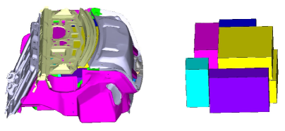
ID	Size	max
A	229mm $\times$ 483mm $\times$ 610mm	4
B	165mm $\times$ 330mm $\times$ 457mm	4
C	229mm $\times$ 406mm $\times$ 660mm	2
D	216mm $\times$ 457mm $\times$ 533mm	2
E	203mm $\times$ 229mm $\times$ 381mm	2
F	178mm $\times$ 356mm $\times$ 533mm	2
G	1143mm $\times$ 204mm $\times$ 204mm	2
H	152mm $\times$ 114mm $\times$ 325mm	20

Figure 1: According to the SAE J1100 standard, a packing consists of suitcases taken from a fixed set. There are six different types of suitcases (A–F), a golf bag (G), and the H-box, which represents additional loose baggage. Some suitcases are allowed twice in the packing, others four times. There may be up to 20 H-boxes, but only in addition to an optimal packing of boxes A–G. Left: Trunk. Middle: Packing. Right: Predefined types of boxes.

In this paper we focus on the SAE J1100 standard. It asks to pack cuboid suitcases, from now on also denoted as boxes, and measures the total volume of the suitcases. The boxes are taken from a fixed set of six types of suitcases, a golf bag, and the so-called H-box, which represents loose baggage. Each box type can only be packed a limited number of times—usually two or four times. The packing is performed in two steps. In the first step it is not allowed to pack any H-box. Only after obtaining an packing with respect to the other boxes, up to 20 H-boxes may be added in a second step. Figure 1 shows a trunk together with a packing and summarizes the important properties.

Until a few years ago, evaluating the size of a trunk was only done manually. Especially for the DIN 70020 standard this is a very tedious task that takes much time and manpower. In order to reduce the cost and to be able to determine the volume of a trunk early in the design process, car manufactures are interested in automated methods. A German car manufacturer sparked the recent interest in such methods, first for the DIN 70020 standard ([7, 8, 11, 13, 14, 15]), and later also for the SAE J1100 standard ([2, 3]). The manufacturer asked for an automatic method that provides a solution not worse than 98% of the best manually obtained packing within 24 hours.

Almost all methods rely on discretizing the trunk, i.e., aligning the trunk with a uniform grid and finding a packing by aligning the boxes with the grid. For the DIN 70020 standard the grid method is the most reasonable approach, because the configuration space, i.e., the set of potential packings, is too large to be tested, if free placement is allowed. The bigger boxes of the SAE J1100 standard yields considerably smaller configuration spaces than the DIN 70020 standard. Still, it is necessary to at least discretize the orientation of the boxes. There has been no research on modeling configuration spaces for objects in three-dimensional space with free placement and orientation, yet. Even the two-dimensional counterpart has been investigated only briefly. The problem is inherently complex.

The major problem of the grid approach for the SAE J1100 standard is to find a suitable grid. The measures of the boxes have non-simple ratios. To make each box fit exactly into the grid, the grid cells must be very small, which increases the complexity of the optimization problem, and therefore also the running time. The grid approach does not pay off any more [1, 14]. Althaus et al. handle the problem by working with a reasonable grid size and allowing the boxes to overlap slightly. The overlap is then resolved with a physical simulation of the contacts [1]. Their algorithm is not guaranteed to find a packing in each run. Instead, they perform several runs, each of which transforms a set of overlapping boxes into a packing. If at least one packing is found, the best packing is returned.

In the following we give an algorithm that does not rely on a grid. We discretize the orientation of the suitcases in the same way as in the grid approach, i.e., we restrict the orientations to the six axis-aligned directions, but our approach allows free positioning of the suitcases within the trunk. Without the grid, configuration space and its description grows considerably. On the other hand, our approach allows to reliably find good packings. Moreover, our approach consists of several tasks, many of which can be performed in parallel. The computation time can be reduced considerably by using multiple machines.

1.1 Outline of Our Algorithm

Reichel proved that the trunk packing problem is NP-hard [14]. Thus, we cannot hope for finding the optimal solution. Our algorithm is based on enumeration. As there are infinitely many different packings, our algorithm does not enumerate packings, but so called packing patterns as introduced by Schepers for the problem of packing small boxes into a large box [16]. Such a pattern bundles a class of packings by fixing a small set of properties. In our scenario, enumerating packing patterns has two advantages:

1. There are only a finite number of packing patterns. Thus, the search tree becomes finite.

2. The properties fixed by a pattern limit the maximum volume of a feasible packing.

Knowing the maximum feasible volume of a packing pattern allows us to prune the search when the maximum feasible volume is not large enough to be interesting. If a pattern is interesting it suffices to check whether there is any feasible packing for the pattern. We solve the feasibility tests by solving a linear program.

The biggest challenge of our approach is to determine a linear program of manageable size. We start by characterizing the feasible positions of the suitcases. For a fixed orientation the area of all feasible positions of suitcase $F$ can be computed with the Minkowski sum, as will be explained in Section 2. Computing the Minkowski sum for each of the six orientations we obtain six polyhedra, which together represent the feasible configurations of $F$.

In a linear program it is preferable to work with convex regions, which can be described as a set of linear inequalities. Then a point is inside the region iff all inequalities are satisfied. If one inequality is not satisfied, then the point lies outside of the region. We therefore describe a region as the difference between its convex hull and a set of convex obstacles. As there are typically a large number of obstacles with a large number of describing inequalities, we simplify the description. Here, it is most important that the simplified representation does not include any additional points. We simplify the representation by transforming the described region into a slightly smaller sub-region that can be described with considerably fewer inequalities (see Section 3).

From the simplified representation of the feasible areas, we can now deduce a linear program of manageable size and start enumerating the packing patterns, as described in Section 4. The algorithm can be summarized as follows.

1. For each box in each orientation determine the region of feasible points for the centers of the boxes.

2. For each region of feasible points $F$, compute its convex hull $C$ and a decomposition of $C-F$ into convex pieces.

3. Simplify the description.

4. Enumerate feasible packing patterns.

Note that we restrict our experiments to the first step of the packing routine, i.e., finding an optimal packing for boxes A–G, and even in this step we ignore the golf bag. Ignoring the golf bag has no technical reasons. We compare our results to the results given i left out the golf bag in their experiments, the

2 Computation of the Feasible Area

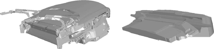
Figure 2: Trunk and the free space of box E (the orientation is fixed) with respect to the trunk. Note that the right picture is enlarged to give a better depiction of the free space.

A configuration space of an object $P$ defines the set of all placements of $P$. The placements may consist of a position and an orientation in a $d$-dimensional work space, with respect to a set of obstacles $Q$ [6]. The placement of $P$ is usually given as the position of a reference point of $P$. This point can be arbitrary. In case of the trunk packing problem it is convenient to use a corner of a suitcase, or, as we do it, the center of the suitcase. The configuration space decomposes into the forbidden space, the set of configurations in which $P$ intersects with $Q$, and the free space, the set of configurations in which $P$ does not intersect $Q$.

We restrict ourselves to a variant of the general problem, where the orientation of the suitcases is limited to the six axis-aligned directions. If the orientation of the object $P$ is fixed, e.g., $P$ is a translational robot, the free space is a subset of the three-dimensional space, which we denote as the feasible area of $P$. It can be computed as the complement of the Minkowski sum $-P\oplus Q=\{p+q:p\in-P,q\in Q\}$, where $-P=\{-p\ |\ p\in P\}$ is the inverted point set of $P$.

In the trunk packing scenario $P$ is a suitcase and $Q$ is the complement of the trunk’s interior, i.e., the trunk’s boundary and the region outside the trunk. We compute the feasible area of a suitcase with respect to a trunk as six complements of Minkowski sums—one for each orientation. Figure 2 shows an example for the Minkowski sum of a trunk and suitcase.

The Minkowski sum of two polyhedra is usually computed by the so-called decomposition method. It decomposes the two polyhedra into convex pieces, computes all pairwise Minkowski sums of the convex pieces, and merges the pairwise sums. In the trunk-packing scenario, one of the polyhedra, the complement of the trunk’s interior, is an infinite set. Unfortunately, none of the few existing implementations of the decomposition method supports infinite point sets [9, 17]. Also, the given input files describe the trunks’ boundary as a surface, which usually has holes. Therefore the trunk cannot be modeled as a solid, which is a necessary precondition for the decomposition method. Unfortunately, we also do not know how to reliably remove the holes from a surface. It seems to be a surprisingly complex problem.

An alternative approach starts by computing the Minkowski sum of the suitcase and the boundary of the trunk, which can be expressed as the union of the Minkowski sums of the suitcase and a facet of the trunk’s boundary. If the holes in the surface are not too large the resulting polyhedron $B$ decomposes the three-dimensional space into three regions: $B$ itself, the region $N$ outside of $B$, and a void $F$ enclosed by $B$ (see Figure 3). It is easy to see, that $F$ coincides with the feasible area.

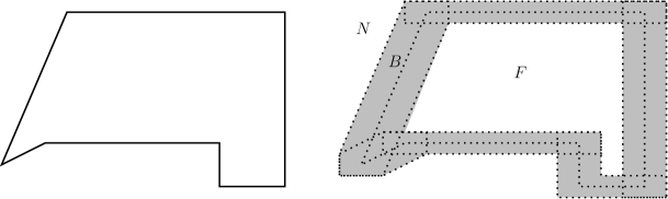
Figure 3: The Minkowski sum of the trunk on the left and a box subdivides the space into three regions, as shown on the right. Region $F$ equals the complement of the Minkowski sum of the trunk’s interior and the (inverted) box.

The trunk models are described by a set of triangles. We compute $B$ as the union of the Minkowski sums of the box and each triangle defining the trunk. The Minkowski sum of a box and a triangle can easily be computed as the convex hull of the vector sums of their vertices. For the union operation we use 3D Nef polyhedra [10] provided by Cgal [4]. The use of Cgal is motivated by robustness issues caused by the multitude of degenerate situations that usually occur during the union step. We also need Cgal in the next step of our algorithm for decomposing a polyhedra into convex pieces, a step that also includes lots of degeneracy problems.

3 Decomposition and Simplification of the Feasible Area

Our enumeration algorithm creates and solves linear programs. One part of the linear programs describes the feasible region. In a linear program it is preferable to work with convex regions, which can be described as the intersection of linear inequalities. We therefore describe a feasible region as its convex hull minus a set of convex obstacles. The convex hull and the difference of the convex hull and the feasible region are computed by Cgal functions. Then we decompose the difference into convex pieces with the decomposition method described in [9].

The data sets generated by the decomposition are too large to find good solutions in reasonable time. In our experiments, the description of the feasible area according to our data format usually comprises several hundred obstacles. The convex hull and a few of the obstacles usually comprise a few hundred half-spaces. The rest of the obstacles have around 6 to 40 facets. Our largest data set has 4904 obstacles and is described by a total of 72554 half-spaces. We therefore need to simplify the data sets, without changing the represented point set too much. Most importantly, we do not want the simplified point set to contain any points outside the feasible area.

We simplify in two steps. In a first step, we merge adjacent obstacles. Because such a union is usually non-convex, we replace the merged obstacles by their combined convex hull. The convex hulls of two adjacent obstacles is larger than the union of the replaced obstacles. Because of the structure of the decomposition—it is a vertical decomposition—it is unlikely that the convex hull of two adjacent obstacles overlaps a third obstacle, and surely it cannot overlap the region outside the convex hull of the feasible area. It usually overlaps a part of the feasible area. Since we want to shrink the represented point set as little as possible, we need ways to measure the size of regions. For this purpose we adapted the code of Mirtich’s volume integration method [12], such that it computes the volume of a cell of a Nef polyhedron. We replace two obstacles by their combined convex hull, if the growth of the convex hull does not exceed a given relative bound of $X\%$ or a given absolute bound of $Ymm^{3}$. The replacement process is performed iteratively as long as we find obstacle pairs that can be joined according to the given percentage and the given fixed volume. Note, that we maintain the volume of the union of each set of joined obstacles. Thus, to test for replacement, we always compare the volume of a convex hull of a set of obstacles, with the volume of their union. To find candidate obstacle pairs, we just iterate in random order over all facets separating two obstacles and check whether they qualify for replacement.

In a second step we reduce the number of describing facets of an obstacle. We iteratively drop facets if as a result the size of the obstacle does not increase much. The growth of an obstacle is measured as the largest distance between a point in the enlarged obstacle and the ignored facet. This quantity can be easily computed by using an LP solver.

4 Enumeration of Feasible Packings

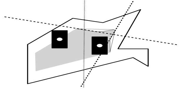
Figure 4: The feasible region of the black rectangle with respect to the (exterior of the) polygon is drawn in gray. It can be represented as the difference of its convex hull and two convex obstacles. The two depicted placements of the rectangle lie within the feasible region as their center points lie within the convex hull of the gray region and fail at least one facet inequality of each obstacle (dashed lines). The dotted line is a separating line of the two placements.

We find packings with the help of a linear-program solver (LP solver). The linear programs that we specify consist of two sets of constraints: constraints that define the convex hull of the configuration spaces, and a packing pattern. A packing pattern specifies a set of boxes together with their orientations, and one separating plane for each box–box and each box–obstacle pair (see Figure 4). A separating plane is a constraint that separates two geometric objects in the 3-dimensional space. In case of the box-box pairs the separating plane is axis-aligned and therefore resembles either a left-of/right-of, in-front-of/behind, or above/under relation. In case of a box–obstacle pair, the constraint is a facet of the obstacle. The set of all packing patterns is infinite, but we only consider patterns, which are either feasible themselves, or which become feasible by removing one box. We call such a packing pattern a candidate pattern.

• $\textnormal{PatternEnumeration}(PartialPattern\ P)$
      1solve LP of P 2if (LP is feasible) 3 if (no intersections exist) 4 save packing if it is the largest found so far 5 for all boxes $b$ and all orientations $d$ 6 $\textnormal{PatternEnumeration}(P\cup b_{d})$ 7 else if (there is a box–box intersection) 8 find box pair $(b_{0},b_{1})$ with largest intersection 9 for all relative orders $r$ 10 compute constraint $c_{r}$ enforcing $r$ on $(b_{0},b_{1})$ 11 $\textnormal{PatternEnumeration}(P\cup c_{r})$ 12 else find box–obstacle pair $(b,o)$ with largest intersection 13 for all defining facets of $o$ 14 compute constraint $c_{o}$ separating $b$ and $o$ 15 $\textnormal{PatternEnumeration}(P\cup c_{o})$

Figure 5: Enumeration of partial packing pattern. The pattern in the first call specifies a box and its orientation. Constraints are only added in the recursive calls.

The set of candidate patterns is finite, but it is still too large to find good packings in a reasonable time. We omit enumerating all patterns as follows. We do not specify all constraints of a pattern, but check subsets of pattern, further on denoted as partial packing pattern. If the LP solver cannot solve the linear program of a partial pattern, we already know that the partial pattern cannot be extended into a solvable pattern. If the LP solver provides a solution to the partial pattern, this solution may not be a solution for the complete pattern. There can still be intersections of box–box or box–obstacle pairs, for which no constraint is specified, yet. We identify those intersection, add a constraint to the partial pattern that prevents one of them, and then let an LP solver solve this new partial pattern. If the LP solver returns a solution without intersections, we have found a packing and can try for a larger set of boxes.

The order, in which we add constraints to a partial pattern, is crucial in keeping the search space as small as possible. It is easy to argue that it is much more efficient to first resolve all box–box intersections and then go on with the box–obstacle intersections than proceeding vice versa. As soon as relations between most of the boxes are specified, the boxes form a big rigid object. Going on with constraints for the box–obstacle pairs moves around this big object until it fits, or until the LP solver cannot provide a solution any more. Most of the times, we expect only few movements until a partial pattern becomes unsolvable. On the other hand, if we start with resolving box–obstacle intersections, the search tree will always be huge. Without constraints for the box–box relations, the box–obstacle constraints will only cause the boxes to overlap one another. We cannot expect to find an unsolvable partial pattern without specifying the box–box relations.

The algorithm is summarized in Figure 5. We left out the details that are necessary to omit redundant enumerations, and the branch-and-bound techniques that omit testing uninteresting packings.

5 Experiments

We implemented our approach in C++ and performed the computations on a machine with a 2.4 GHz AMD Opteron 250 processor and 4 GB RAM. All linear programs were solved with CPLEX 10.0 [5]. We tested our algorithm on three different trunk models, Small (99352 triangles), Medium (66743 triangles), and Large (42182 triangles), which are the same that were used in previous experiments [1, 7].

box	A		B						C				D
orientation	yxz	xyz	zyx	zxy	yzx	xzy	yxz	xyz	yzx	xzy	yxz	xyz	yzx	xzy	yxz	xyz
volume $[dm^{3}]$	21.7	17.3	2.5	1.3	40.1	30.0	74.2	67.0	6.4	1.4	24.3	15.5	1.0	0.2	33.0	29.6
facets $[10^{3}]$	11.4	11.8	4.5	3.2	12.0	10.9	23.3	24.0	7.3	1.7	10.2	11.2	1.9	0.7	14.1	14.5

	E						F				H
	zyx	zxy	yzx	xzy	yxz	xyz	yzx	xzy	yxz	xyz	zyx	zxy	yzx	xzy	yxz	xyz
volume $[dm^{3}]$	31.1	30.3	84.3	74.9	90.7	82.1	25.6	15.4	55.3	46.0	68.2	69.4	138.4	127.0	130.6	118.1
facets $[10^{3}]$	12.5	12.7	20.4	17.8	24.7	22.1	10.7	8.9	19.8	20.4	17.2	18.2	35.6	31.5	32.4	28.7

Table 1: Size of the non-empty feasible areas of Medium and complexity of their description.

The computation of the feasible area of a single suitcase (for one orientation) takes 66 minutes for trunk Small, 36 minutes for Medium, and 69 minutes for trunk Large. The running times do not vary much for different suitcases or orientations. Even the determination of an empty feasible area needs the full computation time. Table 1 lists the volumes and the number of describing facets for the non-empty feasible areas of all boxes in all six orientations with respect to trunk Medium. In the tables we denote the six orientations by permutations of the three coordinate axis. The first letter of a permutation represents the alignment of the longest box side, the third letter represents the alignment of the shortest box side.

For the decomposition and the simplification we did not explicitly measure the running times. From the dates of the created files we can see that decomposition and simplification of a single feasible area takes 1–5 minutes; a whole set of feasible areas of all boxes and all orientations is decomposed and simplified within 2.5–3.5 hours.

		$1000mm^{3}$					$10000mm^{3}$					$100000mm^{3}$
box	orient.	$5\%$	$10\%$	$20\%$	$50\%$	$80\%$	$5\%$	$10\%$	$20\%$	$50\%$	$80\%$	$5\%$	$10\%$	$20\%$	$50\%$	$80\%$
A	yxz	99.5	98.8	97.9	94.4	85.1	98.8	98.3	97.5	94.1	86.0	93.8	93.8	93.8	91.6	84.0
A	xyz	99.7	99.1	97.9	92.5	86.6	98.8	98.4	97.6	92.8	86.5	91.9	91.9	91.9	89.6	84.6
H	zyx	99.8	99.5	98.6	94.6	91.8	99.5	99.4	98.9	94.6	91.9	97.1	97.1	97.1	94.7	91.7
H	zxy	99.8	99.5	98.6	95.4	92.6	99.5	99.3	98.5	95.2	92.9	96.8	96.8	96.6	94.5	91.1
H	yzx	99.8	99.4	98.4	94.6	90.8	99.6	99.3	98.3	94.9	90.8	97.7	97.7	97.4	93.7	90.2
H	xzy	99.8	99.6	98.8	95.6	93.2	99.5	99.3	98.7	95.5	93.5	97.8	97.8	97.7	95.2	93.1
H	yxz	99.7	99.2	98.1	95.0	90.5	99.5	99.1	97.9	95.1	90.4	97.6	97.5	97.2	94.5	88.9
H	xyz	99.8	99.6	98.9	96.0	93.2	99.5	99.4	98.7	96.4	93.1	97.9	97.9	97.6	95.9	93.0
average		99.7	99.4	98.5	94.9	91.3	99.4	99.1	98.3	95.0	91.3	96.6	96.6	96.3	93.9	90.2

		$1000mm^{3}$					$10000mm^{3}$					$100000mm^{3}$
box	orient.	$5\%$	$10\%$	$20\%$	$50\%$	$80\%$	$5\%$	$10\%$	$20\%$	$50\%$	$80\%$	$5\%$	$10\%$	$20\%$	$50\%$	$80\%$
A	yxz	27.2	23.1	19.1	14.5	12.3	22.9	20.1	18.2	15.0	13.5	15.1	15.1	14.8	13.3	11.6
A	xyz	25.5	23.5	18.8	14.4	11.9	19.4	18.8	17.5	14.8	12.7	13.5	13.5	13.5	13.3	11.6
H	zyx	26.1	22.2	17.0	10.7	8.3	22.5	21.5	18.2	10.7	8.3	14.7	14.7	14.1	11.7	9.1
H	zxy	26.9	21.1	17.0	11.4	8.5	21.7	19.5	17.2	11.7	8.5	14.4	14.3	13.7	11.7	9.0
H	yzx	24.8	19.6	14.6	9.3	7.5	20.7	17.9	14.2	10.1	7.4	13.8	13.5	12.7	9.3	7.9
H	xzy	23.2	19.3	14.4	9.2	8.4	19.6	17.8	14.7	10.0	8.6	12.5	12.3	11.3	8.9	8.6
H	yxz	24.5	18.4	14.3	9.8	8.5	20.3	16.9	14.1	9.6	8.6	14.1	14.0	13.5	10.6	8.2
H	xyz	23.7	19.7	15.6	10.8	8.7	19.4	17.9	14.7	11.0	9.3	12.4	12.4	11.4	10.0	8.8
average		25.4	21.2	17.1	11.5	9.8	21.0	18.9	16.5	11.7	9.8	14.0	13.8	13.2	11.2	9.8

Table 2: Impact of first simplification step on the non-empty feasible areas of A and H-box with respect to trunk Medium using parameter values $X=5\%,10\%,20\%,50\%,80\%$ (maximum percentual growth of obstacle union) and $Y=1000mm^{3},10000mm^{3},100000mm^{3}$ (maximum absolute growth of obstacle union). Top: Volume of the represented area after the simplification relative to original volume. Bottom: Number of facets used for describing the feasible area after the simplification relative to original number of facets.

Table 2 shows the effectiveness of our first simplification step. Applying it to trunk Medium, we can reduce the number of defining half-spaces to around 20% while we only loose 1–2% of the feasible area. This trade-off is a bit better for Large and a bit worse for Small.

allowed growth $[mm]$	0	0.1	0.2	0.5	1	2	5	10
obstacle facets	$100\%$	$58\%$	$51\%$	$41\%$	$33\%$	$27\%$	$21\%$	$18\%$

Table 3: Effect of second simplification step applied to the (simplified) feasible area of trunk Small and suitcase D with orientation $zxy$.

Table 3 shows the influence of the second simplification step. On average it additionally reduces the number of defining half-spaces by about $40\%$, $65\%$, or $80\%$, if we allow a growth by $0.1mm$, $1mm$ or $10mm$, respectively.

The enumeration phase of our algorithm does not terminate within $24$ hours for the tested trunks. We terminate the enumeration step after $24$ hours and report the volume of the best packing. Table 4 compares our results with the results of previous approaches. For the trunk Small, we found a better packing than anyone else. For the two other trunks we are not as good as the other approaches. It seems that we perform better when the trunk volume is comparably small. This is probably due the limited number of feasible partial packing patterns that we can enumerate in the given time. On the other hand, the best packing was usually found within one hour. Up to now, we enumerate the packing patterns in a depth-first manner. Changing the order in a clever way, e.g., by determining a measure how promising a certain partial packing pattern is, we expect that the performance of our approach can be improved.

trunk	manual	physics sim.	Minkowski sum
Small	$151.1dm^{3}$	$159.9dm^{3}$	$163.9dm^{3}$
Medium	$264.9dm^{3}$	$266.6dm^{3}$	$263.5dm^{3}$
Large	$335.1dm^{3}$	$358.6dm^{3}$	$321.8dm^{3}$

Table 4: The volume of the best packings found without using the H-boxes by manual packing, by the grid-based method using physics simulation, and by our approach.

Summarizing the running times of the four steps of our algorithm, the computation of the feasible area takes 35–70 minutes for a single box with fixed orientation, which sums up to a total of 24.5–49 hours for all 42 combinations. Then the decomposition and simplification of a complete set takes 2.5–3.5 hours. Finally, the enumeration will probably yield a good solution within 1 hour. In total the computation can last more than 50 hours. The running times become more interesting if we perform computations in parallel. Having six machines instead of one, we can compute the feasible areas in less than 8.5 hours, then create six different simplified point sets using different parameters, and can expect to have a good solution within 13 hours.

6 Conclusion

We have given a new algorithm to compute the volume of a trunk according to the SAE J110 standard as used in the USA. It outperforms previous approaches for small trunks.

In spite of the improvable performance of the computation of the feasible areas, our approach already meets the demands of the German car manufacturer, since many tasks can be performed in parallel. With six machines like ours it is possible to compute the feasible areas and a few sets of their simplified representations on the first half of a day. The other half day suffices to give the LP solver the opportunity to come up with good packings.

We outlined several lines of further research to improve the performance of our algorithm. We are interested in reliable methods to close the surface of a trunk, such that we can design heuristics to speed up the computation of the feasible regions. Furthermore we want to improve the enumeration phase by the development of better upper bounds for the volume that can be obtained by extending a given partial packing pattern together with algorithms to compute these upper bounds and by clever heuristics to scan the large search space.

References

- [1] E. Althaus, T. Baumann, E. Schömer, and K. Werth. Solving geometric packing problems based on physics simulation. Unpublished.
- [2] E. Althaus, T. Baumann, E. Schömer, and K. Werth. Trunk packing revisited. In Proceedings of the 6th International Workshop on Experimental and Efficient Algorithms, (WEA 2007), Lecture Notes in Computer Science, Rome, Italy, 2007.
- [3] J. Cagan and Ding Q. Automated trunk packing with extended pattern search. In Virtual Engineering, Simulation & Optimization, 2003.
- [4] The CGAL Homepage. \path—http://www.cgal.org/—.
- [5] ILOG CPLEX 10.0. \path—http://www.ilog.com/—.
- [6] M. de Berg, M. van Kreveld, M. Overmars, and O. Schwarzkopf. Computational Geometry: Algorithms and Applications. Springer Verlag, 1997.
- [7] F. Eisenbrand, S. Funke, A. Karrenbauer, J. Reichel, and E. Schömer. Packing a trunk: now with a twist! In SPM ’05: Proceedings of the 2005 ACM Symposium on Solid and Physical Modeling, pages 197–206, New York, NY, USA, 2005. ACM.
- [8] F. Eisenbrand, S. Funke, J. Reichel, and E. Schömer. Packing a trunk. In Giuseppe Di Battista and Uri Zwick, editors, Algorithms - ESA 2003: 11th Annual European Symposium, volume 2832 of Lecture Notes in Computer Science, pages 618–629, Budapest, Hungary, September 2003. Springer.
- [9] P. Hachenberger. Exact Minkowksi sums of polyhedra and exact and efficient decomposition of polyhedra in convex pieces. In 15th European Symposium on Algorithms (ESA’07), pages 669–680, 2007.
- [10] P. Hachenberger, L. Kettner, and K. Mehlhorn. Boolean operations on 3D selective Nef complexes: Data structure, algorithms, optimized implementation and experiments. Computational Geometry: Theory and Applications, 38(1–2):64–99, 2007.
- [11] A. Karrenbauer. Packing boxes with arbitrary rotations. Master’s thesis, Universität des Saarlandes, 2004.
- [12] B. Mirtich. Fast and accurate computation of polyhedral mass properties. Journal of Graphics Tools, 1(2):31–50, 1996.
- [13] U. Neumann. Optimierungsverfahren zur normgerechten Volumenbestimmung von Kofferräumen im europäischen Automobilbau. Master’s thesis, Technische Universität Braunschweig, 2006.
- [14] J. Reichel. Combinatorial Approaches for the Trunk Packing Problem. PhD thesis, Universität des Saarlandes, July 2006.
- [15] J. Rieskamp. Automation and optimization of monte carlo based trunk packing. Master’s thesis, Universität des Saarlandes, 2005.
- [16] J. Schepers. Exakte Algorithmen f ur orthogonale Packungsprobleme. PhD thesis, Köln, 1997.
- [17] G. Varadhan and D. Manocha. Accurate Minkowski sum approximation of polyhedral models. In Proc. Comp. Graphics and Appl., 12th Pacific Conf. on (PG’04), pages 392–401. IEEE Computer Society, 2004.