Optimally Training a Cascade Classifier

Abstract

Cascade classifiers are widely used in real-time object detection. Different from conventional classifiers that are designed for a low overall classification error rate, a classifier in each node of the cascade is required to achieve an extremely high detection rate and moderate false positive rate. Although there are a few reported methods addressing this requirement in the context of object detection, there is no a principled feature selection method that explicitly takes into account this asymmetric node learning objective. We provide such an algorithm here. We show a special case of the biased minimax probability machine has the same formulation as the linear asymmetric classifier (LAC) of [1]. We then design a new boosting algorithm that directly optimizes the cost function of LAC. The resulting totally-corrective boosting algorithm is implemented by the column generation technique in convex optimization. Experimental results on object detection verify the effectiveness of the proposed boosting algorithm as a node classifier in cascade object detection, and show performance better than that of the current state-of-the-art.

1 Introduction

Real-time object detection inherently involves searching a large number of candidate image regions for a small number of objects. Processing a single image, for example, can require the interrogation of well over a million scanned windows in order to uncover a single correct detection. This imbalance in the data has an impact on the way that detectors are applied, but also on the training process. This impact is reflected in the need to identify discriminative features from within a large over-complete feature set.

Cascade classifiers have been proposed as a potential solution to the problem of imbalance in the data [2, 3, 4, 5, 6], and have received significant attention due to their speed and accuracy. In this work, we propose a principled method by which to train a boosting-based cascade of classifiers.

The boosting-based cascade approach to object detection was introduced by Viola and Jones [6, 7], and has received significant subsequent attention [8, 9, 10, 11, 12, 13]. It also underpins the current state-of-the-art [1, 2].

The Viola and Jones approach uses a cascade of increasingly complex classifiers, each of which aims to achieve the best possible classification accuracy while achieving an extremely low false negative rate. These classifiers can be seen as forming the nodes of a degenerate binary tree (see Fig. 1) whereby a negative result from any single such node classifier terminates the interrogation of the current patch. Viola and Jones use AdaBoost to train each node classifier in order to achieve the best possible classification accuracy. A low false negative rate is achieved by subsequently adjusting the decision threshold until the desired false negative rate is achieved. This process cannot be guaranteed to produce the best classification accuracy for a given false negative rate.

Under the assumption that each node of the cascade classifier makes independent classification errors, the detection rate and false positive rate of the entire cascade are: $F_{\rm dr}=\prod_{t=1}^{N}d_{t}$ and $F_{\rm fp}=\prod_{t=1}^{N}f_{t}$, respectively, where $d_{t}$ represents the detection rate of classifier $t$, $f_{t}$ the corresponding false positive rate and $N$ the number of nodes. As pointed out in [6, 1], these two equations suggest a node learning objective: Each node should have an extremely high detection rate $d_{t}$ (e.g., $99.7\%$) and a moderate false positive rate $f_{t}$ (e.g., $50\%$). With the above values of $d_{t}$ and $f_{t}$, and a cascade of $N=20$ nodes, then $F_{\rm dr}\approx 94\%$ and $F_{\rm fp}\approx 10^{-6}$, which is a typical design goal.

One drawback of the standard AdaBoost approach to boosting is that it does not take advantage of the cascade classifier’s special structure. AdaBoost only minimizes the overall classification error and does not minimize the number of false negatives. In this sense, the features selected are not optimal for the purpose of rejecting as many negative examples as possible. Viola and Jones proposed a solution to this problem in AsymBoost [7] (and its variants [8, 9, 14, 15]) by modifying the exponential loss function so as to more greatly penalize false negatives. AsymBoost achieves better detection rates than AdaBoost, but still addresses the node learning goal indirectly, and cannot be guaranteed to achieve the optimal solution.

Wu et al. explicitly studied the node learning goal and proposed to use linear asymmetric classifier (LAC) and Fisher linear discriminant analysis (LDA) to adjust the weights on a set of features selected by AdaBoost or AsymBoost [1, 2]. Their experiments indicated that with this post-processing technique the node learning objective can be better met, which is translated into improved detection rates. In Viola and Jones’ framework, boosting is used to select features and at the same time to train a strong classifier. Wu et al.’s work separates these two tasks: AdaBoost or AsymBoost is used to select features; and as a second step, LAC or LDA is used to construct a strong classifier by adjusting the weights of the selected features. The node learning objective is only considered at the second step. At the first step—feature selection—the node learning objective is not explicitly considered at all. We conjecture that further improvement may be gained if the node learning objective is explicitly taken into account at both steps. We thus propose new boosting algorithms to implement this idea and verify this conjecture. A preliminary version of this work was published in Shen et al. [16].

Our major contributions are as follows.

1. Starting from the theory of minimax probability machines (MPMs), we derive a simplified version of the biased minimax probability machine, which has the same formulation as the linear asymmetric classifier of [1]. We thus show the underlying connection between MPM and LAC. Importantly, this new interpretation weakens some of the restrictions on the acceptable input data distribution imposed by LAC.

2. We develop new boosting-like algorithms by directly minimizing the objective function of the linear asymmetric classifier, which results in an algorithm that we label LACBoost. We also propose FisherBoost on the basis of Fished LDA rather than LAC. Both methods may be used to identify the feature set that optimally achieves the node learning goal when training a cascade classifier. To our knowledge, this is the first attempt to design such a feature selection method.

3. LACBoost and FisherBoost share similarities with LPBoost [17] in the sense that both use column generation—a technique originally proposed for large-scale linear programming (LP). Typically, the Lagrange dual problem is solved at each iteration in column generation. We instead solve the primal quadratic programming (QP) problem, which has a special structure and entropic gradient (EG) can be used to solve the problem very efficiently. Compared with general interior-point based QP solvers, EG is much faster.

4. We apply LACBoost and FisherBoost to object detection and better performances are observed over the state-of-the-art methods [1, 2, 18]. The results confirm our conjecture and show the effectiveness of LACBoost and FisherBoost. These methods can be immediately applied to other asymmetric classification problems.

Moreover, we analyze the condition that makes the validity of LAC, and show that the multi-exit cascade might be more suitable for applying LAC learning of [1, 2] (and our LACBoost) rather than Viola-Jones standard cascade.

As observed in Wu et al. [2], in many cases, LDA even performs better than LAC. In our experiments, we have also observed similar phenomena. Paisitkriangkrai et al. [11] empirically showed that LDA’s criterion can be used to achieve better detection results. An explanation of why LDA works so well for object detection is missing in the literature. Here we demonstrate that in the context of object detection, LDA can be seen as a regularized version of LAC in approximation.

The proposed LACBoost/FisherBoost algorithm differs from traditional boosting algorithms in that it does not minimize a loss function. This opens new possibilities for designing new boosting algorithms for special purposes. We have also extended column generation for optimizing nonlinear optimization problems.

Figure 1: Cascade classifiers. The first one is the standard cascade of Viola and Jones [6]. The second one is the multi-exit cascade proposed in [9]. Only those classified as true detection by all nodes will be true targets.

1.1 Related Work

The three components making up the Viola and Jones’ detection approach are:

1. The cascade classifier, which efficiently filters out negative patches in early nodes while maintaining a very high detection rate;

2. AdaBoost that selects informative features and at the same time trains a strong classifier;

3. The use of integral images, which makes the computation of Haar features extremely fast.

This approach has received significant subsequent attention. A number of alternative cascades have been developed including the soft cascade [19], the dynamic cascade [20], and the multi-exit cascade [9]. In this work we have adopted the multi-exit cascade that aims to improve classification performance by using the results of all of the weak classifiers applied to a patch so far in reaching a decision at each node of the tree (see Fig. 1). Thus the $n$-th node classifier uses the results of the weak classifiers associated with node $n$, but also those associated with the previous $n-1$ node classifiers in the cascade. We show below that LAC post-processing can enhance the multi-exit cascade, and that the multi-exit cascade more accurately fulfills the LAC requirement that the margin be drawn from a Gaussian distribution.

There have also been a number of improvements suggested to the Viola and Jones approach to the learning algorithm for constructing a classifier. Wu et al., for example, use fast forward feature selection to accelerate the training procedure [21]. Wu et al. [1] also showed that LAC may be used to deliver better classification performance. Pham and Cham recently proposed online asymmetric boosting that considerably reduces the training time required [8]. By exploiting the feature statistics, Pham and Cham have also designed a fast method to train weak classifiers [22]. Li et al. proposed FloatBoost, which discards redundant weak classifiers during AdaBoost’s greedy selection procedure [10]. Liu and Shum also proposed KLBoost, aiming to select features that maximize the projected Kullback-Leibler divergence and select feature weights by minimizing the classification error [23]. Promising results have also been reported by LogitBoost [24] that employs the logistic regression loss, and GentleBoost [25] that uses adaptive Newton steps to fit the additive model. Multi-instance boosting has been introduced to object detection [26, 27, 28], which does not require exactly labeled locations of the targets in training data.

New features have also been designed for improving the detection performance. Viola and Jones’ Haar features are not sufficiently discriminative for detecting more complex objects like pedestrians, or multi-view faces. Covariance features [24] and histogram of oriented gradients (HOG) [29] have been proposed in this context, and efficient implementation approaches (along the lines of integral images) are developed for each. Shape context, which can also exploit integral images [30], was applied to human detection in thermal images [31]. The local binary pattern (LBP) descriptor and its variants have been shown promising performance on human detection [32, 33]. Recently, effort has been spent on combining complementary features, including: simple concatenation of HOG and LBP [34], combination of heterogeneous local features in a boosted cascade classifier [35], and Bayesian integration of intensity, depth and motion features in a mixture-of-experts model [36].

The paper is organized as follows. We briefly review the concept of minimax probability machine and derive the new simplified version of biased minimax probability machine in Section 2. Linear asymmetric classification and its connection to the minimax probability machine is discussed in Section 3. In Section 4, we show how to design new boosting algorithms (LACBoost and FisherBoost) by rewriting the optimization formulations of LAC and Fisher LDA. The new boosting algorithms are applied to object detection in Section 5 and we conclude the paper in Section 6.

1.2 Notation

The following notation is used. A matrix is denoted by a bold upper-case letter ($\mathbf{X}$); a column vector is denoted by a bold lower-case letter ($\mathbf{x}$). The $i$th row of $\mathbf{X}$ is denoted by $\mathbf{X}_{i:}$ and the $i$th column $\mathbf{X}_{:i}$. The identity matrix is $\bf I$ and its size should be clear from the context. $\bf 1$ and $\bf 0$ are column vectors of $1$’s and $0$’s, respectively. We use $\succcurlyeq,\preccurlyeq$ to denote component-wise inequalities.

Let ${\cal T}=\{(\mathbf{x}_{i},y_{i})\}_{i=1,\cdots,m}$ be the set of training data, where $\mathbf{x}_{i}\in\mathcal{X}$ and $y_{i}\in\{-1,+1\}$, $\forall i$. The training set consists of $m_{1}$ positive training points and $m_{2}$ negative ones; $m_{1}+m_{2}=m$. Let $h(\cdot)\in\mathcal{H}$ be a weak classifier that projects an input vector $\mathbf{x}$ into $\{-1,+1\}$. Note that here we consider only classifiers with discrete outputs although the developed methods can be applied to real-valued weak classifiers too. We assume that $\mathcal{H}$, the set from which $h(\cdot)$ is selected, is finite and has $n$ elements.

Define the matrix $\mathbf{H}^{\cal Z}\in\mathbb{R}^{m\times n}$ such that the $(i,j)$ entry $\mathbf{H}^{\cal Z}_{ij}=h_{j}(\mathbf{x}_{i})$ is the label predicted by weak classifier $h_{j}(\cdot)$ for the datum $\mathbf{x}_{i}$, where $\mathbf{x}_{i}$ the $i$th element of the set ${\cal Z}$. In order to simplify the notation we eliminate the superscript when ${\cal Z}$ is the training set, so $\mathbf{H}^{\cal Z}=\mathbf{H}$. Therefore, each column $\mathbf{H}_{:j}$ of the matrix $\mathbf{H}$ consists of the output of weak classifier $h_{j}(\cdot)$ on all the training data; while each row $\mathbf{H}_{i:}$ contains the outputs of all weak classifiers on the training datum $\mathbf{x}_{i}$. Define similarly the matrix $\mathbf{A}\in\mathbb{R}^{m\times n}$ such that $\mathbf{A}_{ij}=y_{i}h_{j}(\mathbf{x}_{i})$. Note that boosting algorithms entirely depends on the matrix $\mathbf{A}$ and do not directly interact with the training examples. Our following discussion will thus largely focus on the matrix $\mathbf{A}$. We write the vector obtained by multiplying a matrix $\mathbf{A}$ with a vector $\mathbf{w}$ as $\mathbf{A}\mathbf{w}$ and its $i$th entry as $(\mathbf{A}\mathbf{w})_{i}$. If we let $\mathbf{w}$ represent the coefficients of a selected weak classifier then the margin of the training datum $\mathbf{x}_{i}$ is $\rho_{i}=\mathbf{A}_{i:}\mathbf{w}=(\mathbf{A}\mathbf{w})_{i}$ and the vector of such margins for all of the training data is ${\boldsymbol{\rho}}=\mathbf{A}\mathbf{w}$.

2 Minimax Probability Machines

Before we introduce our boosting algorithm, let us briefly review the concept of minimax probability machines (MPM) [37] first.

2.1 Minimax Probability Classifiers

Let $\mathbf{x}_{1}\in\mathbb{R}^{n}$ and $\mathbf{x}_{2}\in\mathbb{R}^{n}$ denote two random vectors drawn from two distributions with means and covariances $({\boldsymbol{\mu}}_{1},{\boldsymbol{\Sigma}}_{1})$ and $({\boldsymbol{\mu}}_{2},{\boldsymbol{\Sigma}}_{2})$, respectively. Here ${\boldsymbol{\mu}}_{1},{\boldsymbol{\mu}}_{2}\in\mathbb{R}^{n}$ and ${\boldsymbol{\Sigma}}_{1},{\boldsymbol{\Sigma}}_{2}\in\mathbb{R}^{n\times n}$. We define the class labels of $\mathbf{x}_{1}$ and $\mathbf{x}_{2}$ as $+1$ and $-1$, w.l.o.g. The minimax probability machine (MPM) seeks a robust separation hyperplane that can separate the two classes of data with the maximal probability. The hyperplane can be expressed as $\mathbf{w}^{\!\top}\mathbf{x}=b$ with $\mathbf{w}\in\mathbb{R}^{n}\backslash\{\bf 0\}$ and $b\in\mathbb{R}$. The problem of identifying the optimal hyperplane may then be formulated as

$$\max_{\mathbf{w},b,\gamma}\,\,\gamma\,\,\,\,{\rm s.t.}\, \left[\inf_{\mathbf{x}_{1}\sim({\boldsymbol{\mu}}_{1},{\boldsymbol{\Sigma}}_{1})}\Pr\{\mathbf{w}^{\!\top}\mathbf{x}_{1}\geq b\}\right]\geq\gamma,$$ (1)

$$\left[\inf_{\mathbf{x}_{2}\sim({\boldsymbol{\mu}}_{2},{\boldsymbol{\Sigma}}_{2})}\Pr\{\mathbf{w}^{\!\top}\mathbf{x}_{2}\leq b\}\right]\geq\gamma.$$

Here $\gamma$ is the lower bound of the classification accuracy (or the worst-case accuracy) on test data. This problem can be transformed into a convex problem, more specifically a second-order cone program (SOCP) [38] and thus can be solved efficiently [37].

Before we present our results, we introduce an important proposition from [39]. Note that we have used different notation.

Proposition 2.1.

For a few different distribution families, the worst-case constraint

$$\left[\inf_{\mathbf{x}\sim({\boldsymbol{\mu}},{\boldsymbol{\Sigma}})}\Pr\{\mathbf{w}^{\!\top}\mathbf{x}\leq b\}\right]\geq\gamma,$$ (2)

can be written as:

1. if $\mathbf{x}\sim({\boldsymbol{\mu}},{\boldsymbol{\Sigma}})$, i.e., $\mathbf{x}$ follows an arbitrary distribution with mean ${\boldsymbol{\mu}}$ and covariance ${\boldsymbol{\Sigma}}$, then

   $$b\geq\mathbf{w}^{\!\top}{\boldsymbol{\mu}}+\sqrt{\tfrac{\gamma}{1-\gamma}}\cdot\sqrt{\mathbf{w}^{\!\top}{\boldsymbol{\Sigma}}\mathbf{w}};$$ (3)

2. if $\mathbf{x}\sim({\boldsymbol{\mu}},{\boldsymbol{\Sigma}})_{\rm S},$ then we have

   $$\begin{cases}b\geq\mathbf{w}^{\!\top}{\boldsymbol{\mu}}+\sqrt{\tfrac{1}{2(1-\gamma)}}\cdot\sqrt{\mathbf{w}^{\!\top}{\boldsymbol{\Sigma}}\mathbf{w}},&\text{if~{}}\gamma\in(0.5,1);\\ b\geq\mathbf{w}^{\!\top}{\boldsymbol{\mu}},&\text{if~{}}\gamma\in(0,0.5];\end{cases}$$ (4)

3. if $\mathbf{x}\sim({\boldsymbol{\mu}},{\boldsymbol{\Sigma}})_{\rm SU}$, then

   $$\begin{cases}b\geq\mathbf{w}^{\!\top}{\boldsymbol{\mu}}+\frac{2}{3}\sqrt{\tfrac{1}{2(1-\gamma)}}\cdot\sqrt{\mathbf{w}^{\!\top}{\boldsymbol{\Sigma}}\mathbf{w}},&\text{if~{}}\gamma\in(0.5,1);\\ b\geq\mathbf{w}^{\!\top}{\boldsymbol{\mu}},&\text{if~{}}\gamma\in(0,0.5];\end{cases}$$ (5)

4. if $\mathbf{x}$ follows a Gaussian distribution with mean ${\boldsymbol{\mu}}$ and covariance ${\boldsymbol{\Sigma}}$, i.e., $\mathbf{x}\sim{\cal G}({\boldsymbol{\mu}},{\boldsymbol{\Sigma}})$, then

   $$b\geq\mathbf{w}^{\!\top}{\boldsymbol{\mu}}+\Phi^{-1}(\gamma)\cdot\sqrt{\mathbf{w}^{\!\top}{\boldsymbol{\Sigma}}\mathbf{w}},$$ (6)

   where $\Phi(\cdot)$ is the cumulative distribution function (c.d.f.) of the standard normal distribution ${\cal G}(0,1)$, and $\Phi^{-1}(\cdot)$ is the inverse function of $\Phi(\cdot)$.

   Two useful observations about $\Phi^{-1}(\cdot)$ are: $\Phi^{-1}(0.5)=0$; and $\Phi^{-1}(\cdot)$ is a monotonically increasing function in its domain.

We omit the proof here and refer the reader to [39] for details.

2.2 Biased Minimax Probability Machines

The formulation (1) assumes that the classification problem is balanced. It attempts to achieve a high recognition accuracy, which assumes that the losses associated with all mis-classifications are identical. However, in many applications this is not the case.

Huang et al. [40] proposed a biased version of MPM through a slight modification of (1), which may be formulated as

$$\max_{\mathbf{w},b,\gamma}\,\,\gamma\,\,\,\,{\rm s.t.}\, \left[\inf_{\mathbf{x}_{1}\sim({\boldsymbol{\mu}}_{1},\Sigma_{1})}\Pr\{\mathbf{w}^{\!\top}\mathbf{x}_{1}\geq b\}\right]\geq\gamma,$$ (7)

$$\left[\inf_{\mathbf{x}_{2}\sim({\boldsymbol{\mu}}_{2},\Sigma_{2})}\Pr\{\mathbf{w}^{\!\top}\mathbf{x}_{2}\leq b\}\right]\geq\gamma_{\circ}.$$

Here $\gamma_{\circ}\in(0,1)$ is a prescribed constant, which is the acceptable classification accuracy for the less important class. The resulting decision hyperplane prioritizes the classification of the important class $\mathbf{x}_{1}$ over that of the less important class $\mathbf{x}_{2}$. Biased MPM is thus expected to perform better in biased classification applications.

Huang et al. showed that (7) can be iteratively solved via solving a sequence of SOCPs using the fractional programming (FP) technique. Clearly it is significantly more computationally demanding to solve (7) than (1).

In this paper we are interested in the special case of $\gamma_{\circ}=0.5$ due to its important application in cascade object detection [6, 1]. In the following discussion, for simplicity, we only consider $\gamma_{\circ}=0.5$ although some algorithms developed may also apply to $\gamma_{\circ}<0.5$.

Next we show how to re-formulate (7) into a simpler quadratic program (QP) based on the recent theoretical results in [39].

2.3 Simplified Biased Minimax Probability Machines

Equation (3) represents the most general of the four cases presented in equations (3) through (6), and is used in MPM [37] and the biased MPM [40] because it does not impose constraints upon the distributions of $\mathbf{x}_{1}$ and $\mathbf{x}_{2}$. On the other hand, one may take advantage of prior knowledge whenever available. For example, it is shown in [1] that in face detection, the weak classifier outputs can be well approximated by Gaussian distributions. Equation (3) does not utilize any this type of a priori information, and hence, for many problems, (3) is too conservative.

Let us consider the special case of $\gamma=0.5$. It is easy to see that the worst-case constraint (2) becomes a simple linear constraint for symmetric, symmetric unimodal, as well as Gaussian distributions. As pointed in [39], such a result is the immediate consequence of symmetry because the worst-case distributions are forced to put probability mass arbitrarily far away on both sides of the mean. In such a case any information about the covariance is neglected.

We now apply this result into biased MPM as represented by (7). Our main result is the following theorem.

Theorem 2.1.

With $\gamma_{\circ}=0.5$, the biased minimax problem (7) can be formulated as an unconstrained problem (16) under the assumption that $\mathbf{x}_{2}$ follows a symmetric distribution. The worst-case classification accuracy for the first class, $\gamma^{\star}$, is obtained by solving

$$\varphi(\gamma^{\star})=\frac{-b^{\star}+{a^{\star}}^{\!\top}{\boldsymbol{\mu}}_{1}}{\sqrt{{\mathbf{w}^{\star}}^{\!\top}\Sigma_{1}\mathbf{w}^{\star}}},$$ (8)

where $\varphi(\cdot)$ is defined in (11); $\{\mathbf{w}^{\star},b^{\star}\}$ is the optimal solution of (15) and (16).

Proof.

The second constraint of (7) is simply

$$b\geq\mathbf{w}^{\!\top}{\boldsymbol{\mu}}_{2}.$$ (9)

The first constraint of (7) can be handled by writing $\mathbf{w}^{\!\top}\mathbf{x}_{1}\geq b$ as $-\mathbf{w}^{\!\top}\mathbf{x}_{1}\leq-b$ and applying the results in Proposition 2.1. It can be written as

$$-b+\mathbf{w}^{\!\top}{\boldsymbol{\mu}}_{1}\geq\varphi(\gamma)\sqrt{\mathbf{w}^{\!\top}\Sigma_{1}\mathbf{w}},$$ (10)

with

$$\varphi(\gamma)=\begin{cases}\sqrt{\frac{\gamma}{1-\gamma}}&\text{ ~{} if~{}}\mathbf{x}_{1}\sim({\boldsymbol{\mu}}_{1},\Sigma_{1}),\\ \sqrt{\frac{1}{2(1-\gamma)}}&\text{ ~{} if~{}}\mathbf{x}_{1}\sim({\boldsymbol{\mu}}_{1},\Sigma_{1})_{\rm S},\\ \frac{2}{3}\sqrt{\frac{1}{2(1-\gamma)}}&\text{ ~{} if~{}}\mathbf{x}_{1}\sim({\boldsymbol{\mu}}_{1},\Sigma_{1})_{\rm SU},\\ \Phi^{-1}(\gamma)&\text{ ~{} if~{}}\mathbf{x}_{1}\sim{\cal G}({\boldsymbol{\mu}}_{1},\Sigma_{1}).\end{cases}$$ (11)

Let us assume that $\Sigma_{1}$ is strictly positive definite (if it is only positive semidefinite, we can always add a small regularization to its diagonal components). From (10) we have

$$\varphi(\gamma)\leq\frac{-b+\mathbf{w}^{\!\top}{\boldsymbol{\mu}}_{1}}{\sqrt{\mathbf{w}^{\!\top}\Sigma_{1}\mathbf{w}}}.$$ (12)

So the optimization problem becomes

$$\max_{\mathbf{w},b,\gamma}\,\gamma,\,\,{\rm s.t.}\,\,\eqref{eq:con1}\text{~{}and~{}}\eqref{eq:11}.$$ (13)

The maximum value of $\gamma$ (which we label $\gamma^{\star}$) is achieved when (12) is strictly an equality. To illustrate this point, let us assume that the maximum is achieved when

$$\varphi(\gamma^{\star})<\frac{-b+\mathbf{w}^{\!\top}{\boldsymbol{\mu}}_{1}}{\sqrt{\mathbf{w}^{\!\top}\Sigma_{1}\mathbf{w}}}.$$

Then a new solution can be obtained by increasing $\gamma^{\star}$ with a positive value such that (12) becomes an equality. Notice that the constraint (9) will not be affected, and the new solution will be better than the previous one. Hence, at the optimum, (8) must be fulfilled.

Because $\varphi(\gamma)$ is monotonically increasing for all the four cases in its domain $(0,1)$ (see Fig. 2), maximizing $\gamma$ is equivalent to maximizing $\varphi(\gamma)$ and this results in

$$\max_{\mathbf{w},b}\,\frac{-b+\mathbf{w}^{\!\top}{\boldsymbol{\mu}}_{1}}{\sqrt{\mathbf{w}^{\!\top}\Sigma_{1}\mathbf{w}}},\,\,{\rm s.t.}\,b\geq\mathbf{w}^{\!\top}{\boldsymbol{\mu}}_{2}.$$ (14)

As in [37, 40], we also have a scale ambiguity: if $(\mathbf{w}^{\star},b^{\star})$ is a solution, $(t\mathbf{w}^{\star},tb^{\star})$ with $t>0$ is also a solution.

An important observation is that the problem (14) must attain the optimum at

$$b=\mathbf{w}^{\!\top}{\boldsymbol{\mu}}_{2}.$$ (15)

Otherwise if $b>\mathbf{w}^{\!\top}{\boldsymbol{\mu}}_{2}$, the optimal value of (14) must be smaller. So we can rewrite (14) as an unconstrained problem

$$\max_{\mathbf{w}}\,\,\frac{\mathbf{w}^{\!\top}({\boldsymbol{\mu}}_{1}-{\boldsymbol{\mu}}_{2})}{\sqrt{\mathbf{w}^{\!\top}{\boldsymbol{\Sigma}}_{1}\mathbf{w}}}.$$ (16)

We have thus shown that, if $\mathbf{x}_{1}$ is distributed according to a symmetric, symmetric unimodal, or Gaussian distribution, the resulting optimization problem is identical. This is not surprising considering the latter two cases are merely special cases of the symmetric distribution family.

At optimality, the inequality (12) becomes an equation, and hence $\gamma^{\star}$ can be obtained as in (8). For ease of exposition, let us denote the fours cases in the right side of (11) as $\varphi_{\rm gnrl}(\cdot)$, $\varphi_{\rm S}(\cdot)$, $\varphi_{\rm SU}(\cdot)$, and $\varphi_{\cal G}(\cdot)$. For $\gamma\in[0.5,1)$, as shown in Fig. 2, we have $\varphi_{\rm gnrl}(\gamma)>\varphi_{\rm S}(\gamma)>\varphi_{\rm SU}(\gamma)>\varphi_{\cal G}(\gamma)$. Therefore, when solving (8) for $\gamma^{\star}$, we have $\gamma^{\star}_{\rm gnrl}<\gamma^{\star}_{\rm S}<\gamma^{\star}_{\rm SU}<\gamma^{\star}_{\cal G}$. That is to say, one can get better accuracy when additional information about the data distribution is available, although the actual optimization problem to be solved is identical. ∎

Figure 2: The function $\varphi(\cdot)$ in (11). The four curves correspond to the four cases. They are all monotonically increasing in $(0,1)$.

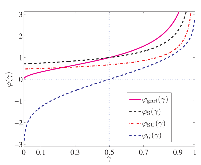
We have derived the biased MPM algorithm from a different perspective. We reveal that only the assumption of symmetric distributions is needed to arrive at a simple unconstrained formulation. Compared the approach in [40], we have used more information to simply the optimization problem. More importantly, as well will show in the next section, this unconstrained formulation enables us to design a new boosting algorithm.

There is a close connection between our algorithm and the linear asymmetric classifier (LAC) in [1]. The resulting problem (16) is exactly the same as LAC in [1]. Removing the inequality in this constraint leads to a problem solvable by eigen-decomposition. We have thus shown that the results of Wu et al. may be generalized from the Gaussian distributions assumed in [1] to symmetric distributions.

It is straightforward to kernelize the linear classifier that we have discussed, following the work of [37, 40]. Here we are more interested, however, in designing a boosting algorithm that takes the biased learning goal into consideration when selecting features.

3 Linear Asymmetric Classification

We have shown that starting from the biased minimax probability machine, we are able to obtain the same optimization formulation as shown in [1], while much weakening the underlying assumption (symmetric distributions versus Gaussian distributions). Before we propose our LACBoost and FisherBoost, however, we provide a brief overview of LAC.

Wu et al. [2] proposed linear asymmetric classification (LAC) as a post-processing step for training nodes in the cascade framework. In [2], it is stated that LAC is guaranteed to reach an optimal solution under the assumption of Gaussian data distributions. We now know that this Gaussianality condition may be relaxed.

Suppose that we have a linear classifier $f(\mathbf{x})={\bf sign}(\mathbf{w}^{\!\top}\mathbf{x}-b)$. We seek a $\{\mathbf{w},b\}$ pair with a very high accuracy on the positive data $\mathbf{x}_{1}$ and a moderate accuracy on the negative $\mathbf{x}_{2}$. This can be expressed as the following problem:

$$\max_{\mathbf{w}\neq{\bf 0},b} \,\Pr_{\mathbf{x}_{1}\sim({\boldsymbol{\mu}}_{1},{\boldsymbol{\Sigma}}_{1})}\{\mathbf{w}^{\!\top}\mathbf{x}_{1}\geq b\},\,\,$$

$${\rm s.t.} \,\Pr_{\mathbf{x}_{2}\sim({\boldsymbol{\mu}}_{2},{\boldsymbol{\Sigma}}_{2})}\{\mathbf{w}^{\!\top}\mathbf{x}_{2}\leq b\}=\lambda,$$ (17)

In [1], $\lambda$ is set to $0.5$ and it is assumed that for any $\mathbf{w}$, $\mathbf{w}^{\!\top}\mathbf{x}_{1}$ is Gaussian and $\mathbf{w}^{\!\top}\mathbf{x}_{2}$ is symmetric, (17) can be approximated by (16). Again, these assumptions may be relaxed as we have shown in the last section. (16) is similar to LDA’s optimization problem

$$\max_{\mathbf{w}\neq\bf 0}\;\;\frac{\mathbf{w}^{\!\top}({\boldsymbol{\mu}}_{1}-{\boldsymbol{\mu}}_{2})}{\sqrt{\mathbf{w}^{\!\top}({\boldsymbol{\Sigma}}_{1}+{\boldsymbol{\Sigma}}_{2})\mathbf{w}}}.$$ (18)

(16) can be solved by eigen-decomposition and a close-formed solution can be derived:

$$\mathbf{w}^{\star}={\boldsymbol{\Sigma}}_{1}^{-1}({\boldsymbol{\mu}}_{1}-{\boldsymbol{\mu}}_{2}),\quad b^{\star}={\mathbf{w}^{\star}}^{{\!\top}}{\boldsymbol{\mu}}_{2}.$$ (19)

On the other hand, each node in cascaded boosting classifiers has the following form:

$$f(\mathbf{x})={\bf sign}(\mathbf{w}^{\!\top}\mathbf{H}(\mathbf{x})-b),$$ (20)

We override the symbol $\mathbf{H}(\mathbf{x})$ here, which denotes the output vector of all weak classifiers over the datum $\mathbf{x}$. We can cast each node as a linear classifier over the feature space constructed by the binary outputs of all weak classifiers. For each node in cascade classifier, we wish to maximize the detection rate while maintaining the false positive rate at a moderate level (for example, around $50.0\%$). That is to say, the problem (16) represents the node learning goal. Boosting algorithms such as AdaBoost can be used as feature selection methods, and LAC used to learn a linear classifier over those binary features chosen by boosting. The advantage of this approach is that LAC considers the asymmetric node learning explicitly.

However, there is a precondition on the validity of LAC that for any $\mathbf{w}$, $\mathbf{w}^{\!\top}\mathbf{x}_{1}$ is a Gaussian and $\mathbf{w}^{\!\top}\mathbf{x}_{2}$ is symmetric. In the case of boosting classifiers, $\mathbf{w}^{\!\top}\mathbf{x}_{1}$ and $\mathbf{w}^{\!\top}\mathbf{x}_{2}$ can be expressed as the margin of positive data and negative data, respectively. Empirically Wu et al. [2] verified that $\mathbf{w}^{\!\top}\mathbf{x}$ is approximately Gaussian for a cascade face detector. We discuss this issue in more detail in Section 5. Shen and Li [41] theoretically proved that under the assumption that weak classifiers are independent, the margin of AdaBoost follows the Gaussian distribution, as long as the number of weak classifiers is sufficiently large. In Section 5 we verify this theoretical result by performing the normality test on nodes with different number of weak classifiers.

4 Constructing Boosting Algorithms from LDA and LAC

In kernel methods, the original data are nonlinearly mapped to a feature space by a mapping function $\Phi(\cdot)$. The function need not be known, however, as rather than being applied to the data directly, it acts instead through the inner product $\Phi(\mathbf{x}_{i})^{\!\top}\Phi(\mathbf{x}_{j})$. In boosting [42], however, the mapping function can be seen as being explicitly known, as $\Phi(\mathbf{x}):\mathbf{x}\mapsto[h_{1}(\mathbf{x}),\dots,h_{n}(\mathbf{x})].$ Let us consider the Fisher LDA case first because the solution to LDA will generalize to LAC straightforwardly, by looking at the similarity between (16) and (18).

Fisher LDA maximizes the between-class variance and minimizes the within-class variance. In the binary-class case, the more general formulation in (18) can be expressed as

$$\max_{\mathbf{w}}\;\;\frac{({\boldsymbol{\mu}}_{1}-{\boldsymbol{\mu}}_{2})^{2}}{\sigma_{1}+\sigma_{2}}=\frac{\mathbf{w}^{\!\top}\mathbf{C}_{b}\mathbf{w}}{\mathbf{w}^{\!\top}\mathbf{C}_{w}\mathbf{w}},$$ (21)

where $\mathbf{C}_{b}$ and $\mathbf{C}_{w}$ are the between-class and within-class scatter matrices; ${\boldsymbol{\mu}}_{1}$ and ${\boldsymbol{\mu}}_{2}$ are the projected centers of the two classes. The above problem can be equivalently reformulated as

$$\min_{\mathbf{w}}\;\;\mathbf{w}^{\!\top}\mathbf{C}_{w}\mathbf{w}-\theta({\boldsymbol{\mu}}_{1}-{\boldsymbol{\mu}}_{2})$$ (22)

for some certain constant $\theta$ and under the assumption that ${\boldsymbol{\mu}}_{1}-{\boldsymbol{\mu}}_{2}\geq 0$. Now in the feature space, our data are $\Phi(\mathbf{x}_{i})$, $i=1\dots m$. Define the vectors $\boldsymbol{e},\boldsymbol{e}_{1},\boldsymbol{e}_{2}\in\mathbb{R}^{m}$ such that $\boldsymbol{e}=\boldsymbol{e}_{1}+\boldsymbol{e}_{2}$, the $i$-th entry of $\boldsymbol{e}_{1}$ is $1/m_{1}$ if $y_{i}=+1$ and $0$ otherwise, and the $i$-th entry of $\boldsymbol{e}_{2}$ is $1/m_{2}$ if $y_{i}=-1$ and $0$ otherwise. We then see that

$${\boldsymbol{\mu}}_{1} =\frac{1}{m_{1}}\mathbf{w}^{\!\top}\sum_{y_{i}=1}\Phi(\mathbf{x}_{i})=\frac{1}{m_{1}}\sum_{y_{i}=1}\mathbf{A}_{i:}\mathbf{w}$$

$$=\frac{1}{m_{1}}\sum_{y_{i}=1}(\mathbf{A}\mathbf{w})_{i}=\boldsymbol{e}_{1}^{\!\top}\mathbf{A}\mathbf{w},$$ (23)

and

$${\boldsymbol{\mu}}_{2} =\frac{1}{m_{2}}\mathbf{w}^{\!\top}\sum_{y_{i}=-1}\Phi(\mathbf{x}_{i})=\frac{1}{m_{2}}\sum_{y_{i}=-1}\mathbf{H}_{i:}\mathbf{w}=-\boldsymbol{e}_{2}^{\!\top}\mathbf{A}\mathbf{w},$$ (24)

For ease of exposition we order the training data according to their labels so the vector $\boldsymbol{e}\in\mathbb{R}^{m}$:

$$\boldsymbol{e}=[1/m_{1},\cdots,1/m_{2},\cdots]^{\!\top},$$ (25)

and the first $m_{1}$ components of ${\boldsymbol{\rho}}$ correspond to the positive training data and the remaining ones correspond to the $m_{2}$ negative data. We now see that ${\boldsymbol{\mu}}_{1}-{\boldsymbol{\mu}}_{2}=\boldsymbol{e}^{\!\top}{\boldsymbol{\rho}}$, $\mathbf{C}_{w}={m_{1}}/{m}\cdot{\boldsymbol{\Sigma}}_{1}+{m_{2}}/{m}\cdot{\boldsymbol{\Sigma}}_{2}$ with ${\boldsymbol{\Sigma}}_{1,2}$ the covariance matrices. Noting that

$$\mathbf{w}^{\!\top}{\boldsymbol{\Sigma}}_{1,2}\mathbf{w}=\frac{1}{m_{1,2}(m_{1,2}-1)}\sum_{i>k,y_{i}=y_{k}=\pm 1}(\rho_{i}-\rho_{k})^{2},$$

we can easily rewrite the original problem (21) (and (22)) into:

$$\min_{\mathbf{w},{\boldsymbol{\rho}}}~{} \tfrac{1}{2}{\boldsymbol{\rho}}^{\!\top}\mathbf{Q}{\boldsymbol{\rho}}-\theta\boldsymbol{e}^{\!\top}{\boldsymbol{\rho}},$$

$$\quad{\rm s.t.}~{} \mathbf{w}\succcurlyeq{\bf 0},{\bf 1}^{\!\top}\mathbf{w}=1,$$

$${\rho}_{i}=(\mathbf{A}\mathbf{w})_{i},i=1,\cdots,m.$$ (26)

Here $\mathbf{Q}=\begin{bmatrix}\mathbf{Q}_{1}&{\bf 0}\\ {\bf 0}&\mathbf{Q}_{2}\end{bmatrix}$ is a block matrix with

$$\mathbf{Q}_{1}=\begin{bmatrix}\tfrac{1}{m}&-\tfrac{1}{m(m_{1}-1)}&\ldots&-\tfrac{1}{m(m_{1}-1)}\\ -\tfrac{1}{m(m_{1}-1)}&\tfrac{1}{m}&\ldots&-\tfrac{1}{m(m_{1}-1)}\\ \vdots&\vdots&\ddots&\vdots\\ -\tfrac{1}{m(m_{1}-1)}&-\tfrac{1}{m(m_{1}-1)}&\ldots&\tfrac{1}{m}\end{bmatrix},$$

and $\mathbf{Q}_{2}$ is similarly defined by replacing $m_{1}$ with $m_{2}$ in $\mathbf{Q}_{1}$:

$$\mathbf{Q}_{2}=\begin{bmatrix}\tfrac{1}{m}&-\tfrac{1}{m(m_{2}-1)}&\ldots&-\tfrac{1}{m(m_{2}-1)}\\ -\tfrac{1}{m(m_{2}-1)}&\tfrac{1}{m}&\ldots&-\tfrac{1}{m(m_{2}-1)}\\ \vdots&\vdots&\ddots&\vdots\\ -\tfrac{1}{m(m_{2}-1)}&-\tfrac{1}{m(m_{2}-1)}&\ldots&\tfrac{1}{m}\end{bmatrix}.$$

Also note that we have introduced a constant $\frac{1}{2}$ before the quadratic term for convenience. The normalization constraint ${\bf 1}^{\!\top}\mathbf{w}=1$ removes the scale ambiguity of $\mathbf{w}$. Without it the problem is ill-posed.

We see from the form of (16) that the covariance of the negative data is not involved in LAC and thus that if we set $\mathbf{Q}=\begin{bmatrix}\mathbf{Q}_{1}&{\bf 0}\\ {\bf 0}&\bf 0\end{bmatrix}$ then (26) becomes the optimization problem of LAC.

There may be extremely (or even infinitely) many weak classifiers in $\mathcal{H}$, the set from which $h(\cdot)$ is selected, meaning that the dimension of the optimization variable $\mathbf{w}$ may also be extremely large. So (26) is a semi-infinite quadratic program (SIQP). We show how column generation can be used to solve this problem. To make column generation applicable, we need to derive a specific Lagrange dual of the primal problem.

4.1 The Lagrange Dual Problem

We now derive the Lagrange dual of the quadratic problem (26). Although we are only interested in the variable $\mathbf{w}$, we need to keep the auxiliary variable $\boldsymbol{\rho}$ in order to obtain a meaningful dual problem. The Lagrangian of (26) is

$$L(\underbrace{\mathbf{w},{\boldsymbol{\rho}}}_{\rm primal},\underbrace{\mathbf{u},r}_{\rm dual}) =\tfrac{1}{2}{\boldsymbol{\rho}}^{\!\top}\mathbf{Q}{\boldsymbol{\rho}}-\theta\boldsymbol{e}^{\!\top}{\boldsymbol{\rho}}+\mathbf{u}^{\!\top}({\boldsymbol{\rho}}-\mathbf{A}\mathbf{w})-\mathbf{q}^{\!\top}\mathbf{w}$$

$$+r({\bf 1}^{\!\top}\mathbf{w}-1),$$

with $\mathbf{q}\succcurlyeq\bf 0$. $\sup_{\mathbf{u},r}\inf_{\mathbf{w},{\boldsymbol{\rho}}}L(\mathbf{w},{{\boldsymbol{\rho}}},\mathbf{u},r)$ gives the following Lagrange dual:

$$\max_{\mathbf{u},r}~{} -r-\overbrace{\tfrac{1}{2}(\mathbf{u}-\theta\boldsymbol{e})^{\!\top}\mathbf{Q}^{-1}(\mathbf{u}-\theta\boldsymbol{e})}^{\rm regularization},{\rm\;\;s.t.}~{}\sum_{i=1}^{m}u_{i}\mathbf{A}_{i:}\preccurlyeq r{\bf 1}^{\!\top}.$$ (27)

In our case, $\mathbf{Q}$ is rank-deficient and its inverse does not exist (for both LDA and LAC). We can simply regularize $\mathbf{Q}$ with $\mathbf{Q}+\delta{\bf I}$ with $\delta$ a small positive constant. Actually, $\mathbf{Q}$ is a diagonally dominant matrix but not strict diagonal dominance. So $\mathbf{Q}+\delta{\bf I}$ with any $\delta>0$ is strict diagonal dominance and by the Gershgorin circle theorem, a strictly diagonally dominant matrix must be invertible.

One of the KKT optimality conditions between the dual and primal

$${\boldsymbol{\rho}}^{\star}=-\mathbf{Q}^{-1}(\mathbf{u}^{\star}-\theta\boldsymbol{e}),$$ (28)

which can be used to establish the connection between the dual optimum and the primal optimum. This is obtained by the fact that the gradient of $L$ w.r.t. ${\boldsymbol{\rho}}$ must vanish at the optimum, ${\partial L}/{\partial\rho_{i}}=0$, $\forall i=1\cdots n$.

Problem (27) can be viewed as a regularized LPBoost problem. Compared with the hard-margin LPBoost [17], the only difference is the regularization term in the cost function. The duality gap between the primal (26) and the dual (27) is zero. In other words, the solutions of (26) and (27) coincide. Instead of solving (26) directly, one calculates the most violated constraint in (27) iteratively for the current solution and adds this constraint to the optimization problem. In theory, any column that violates dual feasibility can be added. To speed up the convergence, we add the most violated constraint by solving the following problem:

$$h^{\prime}(\cdot)={\rm argmax}_{h(\cdot)}~{}\sum_{i=1}^{m}u_{i}y_{i}h(\mathbf{x}_{i}).$$ (29)

This is exactly the same as the one that standard AdaBoost and LPBoost use for producing the best weak classifier. That is to say, to find the weak classifier that has minimum weighted training error. We summarize the LACBoost/FisherBoost algorithm in Algorithm 1. By simply changing $\mathbf{Q}_{2}$, Algorithm 1 can be used to train either LACBoost or FisherBoost. Note that to obtain an actual strong classifier, one may need to include an offset $b$, i.e. the final classifier is $\sum_{j=1}^{n}h_{j}(\mathbf{x})-b$ because from the cost function of our algorithm (22), we can see that the cost function itself does not minimize any classification error. It only finds a projection direction in which the data can be maximally separated. A simple line search can find an optimal $b$. Moreover, when training a cascade, we need to tune this offset anyway as shown in (20).

The convergence of Algorithm 1 is guaranteed by general column generation or cutting-plane algorithms, which is easy to establish. When a new $h^{\prime}(\cdot)$ that violates dual feasibility is added, the new optimal value of the dual problem (maximization) would decrease. Accordingly, the optimal value of its primal problem decreases too because they have the same optimal value due to zero duality gap. Moreover the primal cost function is convex, therefore in the end it converges to the global minimum.

Algorithm 1 Column generation for SIQP.

Input:

Labeled training data $(\mathbf{x}_{i},y_{i}),i=1\cdots m$; termination threshold $\varepsilon>0$; regularization parameter $\theta$; maximum number of iterations $n_{\rm max}$.

Initialization: $m=0$; $\mathbf{w}={\bf 0}$; and $u_{i}=\frac{1}{m}$, $i=1$$\cdots$$m$.

for $\mathrm{iteration}=1:n_{\mathrm{max}}$ do

  $-\,$ Check for the optimality: if $\mathrm{iteration}>1$ and $\sum_{i=1}^{m}u_{i}y_{i}h^{\prime}(\mathbf{x}_{i})<r+\varepsilon$, then     break; and the problem is solved; $-\,$ Add $h^{\prime}(\cdot)$ to the restricted master problem, which corresponds to a new constraint in the dual; $-\,$ Solve the dual problem (27) (or the primal problem (26)) and update $r$ and $u_{i}$ ($i=1\cdots m$). $-\,$ Increment the number of weak classifiers $n=n+1$.   Output: The selected features are $h_{1},h_{2},\dots,h_{n}$. The final strong classifier is: $F(\mathbf{x})=\textstyle\sum_{j=1}^{n}w_{j}h_{j}(\mathbf{x})-b$. Here the offset $b$ can be learned by a simple search.

At each iteration of column generation, in theory, we can solve either the dual (27) or the primal problem (26). However, in practice, it could be much faster to solve the primal problem because

1. Generally, the primal problem has a smaller size, hence faster to solve. The number of variables of (27) is $m$ at each iteration, while the number of variables is the number of iterations for the primal problem. For example, in Viola-Jones’ face detection framework, the number of training data $m=10,000$ and $n_{\rm max}=200$. In other words, the primal problem has at most $200$ variables in this case;

2. The dual problem is a standard QP problem. It has no special structure to exploit. As we will show, the primal problem belongs to a special class of problems and can be efficiently solved using entropic/exponentiated gradient descent (EG) [43, 44]. A fast QP solver is extremely important for training a object detector because we need to the solve a few thousand QP problems.

We can recover both of the dual variables $\mathbf{u}^{\star},r^{\star}$ easily from the primal variable $\mathbf{w}^{\star}$:

$$\mathbf{u}^{\star} =-\mathbf{Q}{\boldsymbol{\rho}}^{\star}+\theta\boldsymbol{e};$$ (30)

$$r^{\star} =\max_{j=1\dots n}\bigl{\{}\textstyle\sum_{i=1}^{m}u_{i}^{\star}\mathbf{A}_{ij}\bigr{\}}.$$ (31)

The second equation is obtained by the fact that in the dual problem’s constraints, at optimum, there must exist at least one $u_{i}^{\star}$ such that the equality holds. That is to say, $r^{\star}$ is the largest edge over all weak classifiers.

We give a brief introduction to the EG algorithm before we proceed. Let us first define the unit simplex $\Delta_{n}=\{\mathbf{w}\in\mathbb{R}^{n}:{\bf 1}^{\!\top}\mathbf{w}=1,\mathbf{w}\succcurlyeq{\bf 0}\}$. EG efficiently solves the convex optimization problem

$$\min_{\mathbf{w}}\,\,\,f(\mathbf{w}),\,{\rm s.t.}\,\,\mathbf{w}\in\Delta_{n},$$ (32)

under the assumption that the objective function $f(\cdot)$ is a convex Lipschitz continuous function with Lipschitz constant $L_{f}$ w.r.t. a fixed given norm $\lVert\cdot\rVert$. The mathematical definition of $L_{f}$ is that $|f(\mathbf{w})-f(\mathbf{z})|\leq L_{f}\lVert\mathbf{x}-\mathbf{z}\rVert$ holds for any $\mathbf{x},\mathbf{z}$ in the domain of $f(\cdot)$. The EG algorithm is very simple:

1. Initialize with $\mathbf{w}^{0}\in\text{the interior of }\Delta_{n}$;

2. Generate the sequence $\{\mathbf{w}^{k}\}$, $k=1,2,\cdots$ with:

   $$\mathbf{w}^{k}_{j}=\frac{\mathbf{w}^{k-1}_{j}\exp[-\tau_{k}f^{\prime}_{j}(\mathbf{w}^{k-1})]}{\sum_{j=1}^{n}\mathbf{w}^{k-1}_{j}\exp[-\tau_{k}f^{\prime}_{j}(\mathbf{w}^{k-1})]}.$$ (33)

   Here $\tau_{k}$ is the step-size. $f^{\prime}(\mathbf{w})=[f_{1}^{\prime}(\mathbf{w}),\dots,f_{n}^{\prime}(\mathbf{w})]^{\!\top}$ is the gradient of $f(\cdot)$;

3. Stop if some stopping criteria are met.

The learning step-size can be determined by $\tau_{k}=\frac{\sqrt{2\log n}}{L_{f}}\frac{1}{\sqrt{k}},$ following [43]. In [44], the authors have used a simpler strategy to set the learning rate.

EG is a very useful tool for solving large-scale convex minimization problems over the unit simplex. Compared with standard QP solvers like Mosek [45], EG is much faster. EG makes it possible to train a detector using almost the same amount of time as using standard AdaBoost as the majority of time is spent on weak classifier training and bootstrapping.

In the case that $m_{1}\gg 1$,

$$\mathbf{Q}_{1}=\frac{1}{m}\begin{bmatrix}1&-\tfrac{1}{m_{1}-1}&\ldots&-\tfrac{1}{m_{1}-1}\\ -\tfrac{1}{m_{1}-1}&1&\ldots&-\tfrac{1}{m_{1}-1}\\ \vdots&\vdots&\ddots&\vdots\\ -\tfrac{1}{m_{1}-1}&-\tfrac{1}{m_{1}-1}&\ldots&1\end{bmatrix}\approx\frac{1}{m}\bf I.$$

Similarly, for LDA, $\mathbf{Q}_{2}\approx\frac{1}{m}\bf I$ when $m_{2}\gg 1$. Hence,

$$\mathbf{Q}\approx\begin{cases}\frac{1}{m}\bf I;&\text{for Fisher LDA},\\ \frac{1}{m}\begin{bmatrix}{\bf I}&{\bf 0}\\ {\bf 0}&{\bf 0}\end{bmatrix},&\text{for LAC}.\end{cases}$$ (34)

Therefore, the problems involved can be simplified when $m_{1}\gg 1$ and $m_{2}\gg 1$ hold. The primal problem (26) equals

$$\min_{\mathbf{w},{\boldsymbol{\rho}}}~{} \tfrac{1}{2}\mathbf{w}^{\!\top}(\mathbf{A}^{\!\top}\mathbf{Q}\mathbf{A})\mathbf{w}-(\theta\boldsymbol{e}^{\!\top}\mathbf{A})\mathbf{w},\;\;{\rm s.t.}\;\mathbf{w}\in\Delta_{n}.$$ (35)

We can efficiently solve (35) using the EG method. In EG there is an important parameter $L_{f}$, which is used to determine the step-size. $L_{f}$ can be determined by the $\ell_{\infty}$-norm of $|f^{\prime}(\mathbf{w})|$. In our case $f^{\prime}(\mathbf{w})$ is a linear function, which is trivial to compute. The convergence of EG is guaranteed; see [43] for details.

In summary, when using EG to solve the primal problem, Line $5$ of Algorithm 1 is:

$-\,$ Solve the primal problem (35) using EG, and update the dual variables $\mathbf{u}$ with (30), and $r$ with (31).

5 Experiments

In this section, we first show an experiment on toy data and then apply the proposed methods to face detection and pedestrian detection.

5.1 Synthetic Testing

Figure 3: Decision boundaries of AdaBoost (top) and FisherBoost (bottom) on $2$D artificial data (positive data represented by $\square$’s and negative data by $\times$’s). Weak classifiers are decision stumps. In this case, FisherBoost intends to correctly classify more positive data in this case.

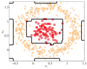
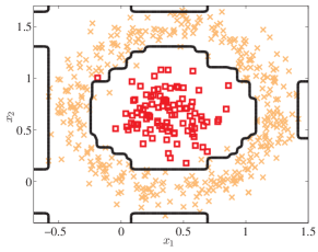
First, let us show a simple example on a synthetic dataset (more negative data than positive data) to illustrate the difference between FisherBoost and AdaBoost. Fig. 3 demonstrates the subtle difference of the classification boundaries obtained by AdaBoost and FisherBoost when applied to these data. We can see that FisherBoost places more emphasis on correctly classifying positive data points than does AdaBoost. This might be due to the fact that AdaBoost only optimizes the overall classification accuracy. This finding is consistent with the result in [11].

Figure 4: Normality test (normal probability plot) for the face data’s margin distribution of nodes $1$, $2$, $3$. The $3$ nodes contains $7$, $22$, $52$ weak classifiers respectively. Curves close to a straight line mean close to a Gaussian.

5.2 Face Detection Using a Cascade Classifier

In this section, we compare FisherBoost and LACBoost with the state-of-the-art in face detection.

We first show some results about the validity of LAC (and Fisher LDA) post-processing for improving node learning in object detection.

Algorithm 2 The procedure for training a multi-exit cascade with LACBoost or FisherBoost.

Input:

$-\,$ A training set with $m$ examples, which are ordered by their labels ($m_{1}$ positive examples followed by $m_{2}$ negative examples);

$-\,$ $d_{\mathrm{min}}$: minimum acceptable detection rate per node;

$-\,$ $f_{\mathrm{max}}$: maximum acceptable false positive rate per node;

$-\,$ $F_{\mathrm{fp}}$: target overall false positive rate.

Initialize:

$t=0$; (node index)

$n=0$; (total selected weak classifiers up to the current node)

$D_{t}=1$; $F_{t}=1$. (overall detection rate and false positive rate up to the current node)

while $F_{\mathrm{fp}}<F_{t}$ do

  $t=t+1$; (increment node index) while $d_{t}<d_{\mathrm{min}}$ do   (current detection rate $d_{t}$ is not acceptable yet) $-\,$ $n=n+1$, and generate a weak classifier and update all the weak classifiers’ linear coefficient using LACBoost or FisherBoost. $-\,$ Adjust threshold $b$ of the current boosted strong classifier $$F^{t}({\bf x})=\sum_{j=1}^{n}w^{t}_{j}h_{j}({\bf x})-b$$ such that $f_{t}\approx f_{\mathrm{max}}$. $-\,$ Update the detection rate of the current node $d_{t}$ with the learned boosted classifier.   Update $D_{t+1}=D_{t}\times d_{t}$; $F_{t+1}=F_{t}\times f_{t}$ Remove correctly classified negative samples from negative training set. if $F_{\mathrm{fp}}<F_{t}$ then   Evaluate the current cascaded classifier on the negative images and add misclassified samples into the negative training set; (bootstrap)     Output: A multi-exit cascade classifier with $n$ weak classifiers and $t$ nodes.

The algorithm for training a multi-exit cascade is shown in Algorithm 2.

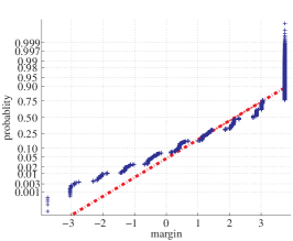
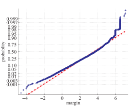
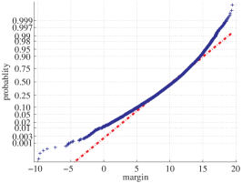
As is described above, LAC and LDA assume that the margins of training data associated with the node classifiers in such a cascade exhibit a Gaussian distribution. In order to evaluate the degree to which this is true for the face detection task we show in Fig. 4 normal probability plots of the margins of the positive training data for each of the first three node classifiers in a multi-exit LAC cascade. The figure shows that the larger the number of weak classifiers used the more closely the margins follow a Gaussian distribution. From this we infer that LAC, Fisher LDA post-processing, (and thus LACBoost and FisherBoost) can be expected to achieve a better performance when a larger number of weak classifiers are used. We therefore apply LAC/LDA only within the later nodes (for example, $9$ onwards) of a multi-exit cascade as these nodes contain more weak classifiers. Because the late nodes of a multi-exit cascade contain more weak classifiers than the standard Viola-Jones’ cascade, we conjecture that the multi-exit cascade might meet the Gaussianity requirement better. We have compared multi-exit cascades with LDA/LAC post-processing against standard cascades with LDA/LAC post-processing in [2] and slightly improved performances were obtained.

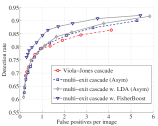
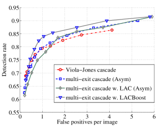
Six methods are evaluated with the multi-exit cascade framework [9], which are AdaBoost with LAC post-processing, or LDA post-processing, AsymBoost with LAC or LDA post-processing [2], and our FisherBoost, LACBoost. We have also implemented Viola-Jones’ face detector as the baseline [6]. As in [6], five basic types of Haar-like features are calculated, resulting in a $162,336$ dimensional over-complete feature set on an image of $24\times 24$ pixels. To speed up the weak classifier training, as in [2], we uniformly sample $10\%$ of features for training weak classifiers (decision stumps). The training data are $9,832$ mirrored $24\times 24$ face images ($5,000$ for training and $4,832$ for validation) and $7,323$ large background images, which are the same as in [2]. The face images for training are provided by Viola and Jones’ work—the same as the face training data used in [6].

Figure 5: Node performances on the validation data for face detection. “Ada” means that features are selected using AdaBoost; “Asym” means that features are selected using AsymBoost.

Multi-exit cascades with $22$ exits and $2,923$ weak classifiers are trained with each of the methods listed above. In order to ensure a fair comparison, we have used the same cascade structure and same number of weak classifiers for all the compared learning methods. The indexes of exits are pre-set to simplify the training procedure.

For our FisherBoost and LACBoost, we have an important parameter $\theta$, which is chosen from $\{\frac{1}{10},\frac{1}{12},\frac{1}{15},$ $\frac{1}{20},\frac{1}{25},\frac{1}{30},$ $\frac{1}{40},\frac{1}{50}\}$. We have not carefully tuned this parameter using cross-validation. Instead, we train a $10$-node cascade for each candidate $\theta$, and choose the one with the best training accuracy. At each exit, negative examples misclassified by current cascade are discarded, and new negative examples are bootstrapped from the background images pool. In total, billions of negative examples are extracted from the pool. The positive training data and validation data keep unchanged during the training process.

Our experiments are performed on a workstation with $8$ Intel Xeon E$5520$ CPUs and $32$GB RAM. It takes about $3$ hours to train the multi-exit cascade with AdaBoost or AsymBoost. For FisherBoost and LACBoost, it takes less than $4$ hours to train a complete multi-exit cascade. In other words, our EG algorithm takes less than $1$ hour to solve the primal QP problem (we need to solve a QP at each iteration). As an estimation of the computational complexity, suppose that the number of training examples is $m$, number of weak classifiers is $n$. At each iteration of the cascade training, the complexity of solving the primal QP using EG is $O(mn+kn^{2})$ with $k$ the iterations needed for EG’s convergence. The complexity for training the weak classifier is $O(md)$ with $d$ the number of all Haar-feature patterns. In our experiment, $m=10,000$, $n\approx 2900$, $d=160,000$, $k<500$. So the majority of the computational cost of the training process is bound up in the weak classifier training.

We have also experimentally observed the speedup of EG against standard QP solvers. We solve the primal QP defined by (35) using EG and Mosek [45]. The QP’s size is $1,000$ variables. With the same accuracy tolerance (Mosek’s primal-dual gap is set to $10^{-7}$ and EG’s convergence tolerance is also set to $10^{-7}$), Mosek takes $1.22$ seconds and EG is $0.0541$ seconds on our standard Desktop. So EG is about $20$ times faster. Moreover, at iteration $n+1$ of training the cascade, EG can take advantage of the last iteration’s solution by starting EG from a small perturbation of the previous solution. Such a warm-start gains a $5$ to $10\times$ speedup in our experiment, while there is no off-the-shelf warm-start QP solvers available yet.

We evaluate the detection performance on the MIT+CMU frontal face test set. This dataset is made up of $507$ frontal faces in $130$ images with different background.

If one positive output has less than $50\%$ variation of shift and scale from the ground-truth, we treat it as a true positive, otherwise a false positive.

In the test phase, the scale factor of the scanning window is set to $1.2$ and the stride step is set to $1$ pixel. Two performance metrics are used here: one for each node and one for the entire cascade. The node metric is how well the classifiers meet the node learning objective, which provides useful information about the capability of each method to achieve the node learning goal. The cascade metric uses the receiver operating characteristic (ROC) to compare the entire cascade’s performance. Note that multiple factors impact on the cascade’s performance, however, including: the classifier set, the cascade structure, bootstrapping etc.

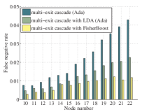
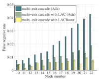
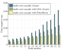
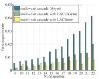
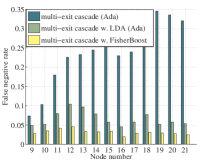
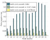
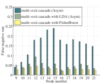
Fig. 5 shows the false-negative rates for the various forms of node classifiers when applied to the MIT+CMU face data. The figure shows that FisherBoost and LACBoost exhibit significantly better node classification performance than the post-processing approach, which verifies the advantage of selecting features on the basis of the node learning goal. Note that the performance of FisherBoost and LACBoost is very similar, but also that LDA or LAC post-processing can considerably reduce the false negative rates over the standard Viol-Jones’ approach, which corresponds with the findings in [2].

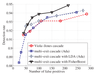
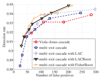
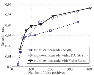
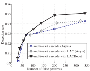
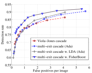
The ROC curves in Fig. 6 demonstrate the superior performance of FisherBoost and LACBoost in the face detection task. Fig. 6 also shows that LACBoost does not outperform FisherBoost in all cases, in contract to the node performance (detection rate) results. Many factors impact upon final performance, however, and these sporadic results are not seen as being particularly indicative. One possible cause is that LAC makes the assumption of Gaussianity and symmetry data distributions, which may not hold well in the early nodes. Wu et al. have observed the same phenomenon that LAC post-processing does not outperform LDA post-processing in some cases.

The error reduction results of FisherBoost and LACBoost in Fig. 6 are not as great as those in Fig. 5. This might be explained by the fact that the cascade and negative data bootstrapping are compensating for the inferior node classifier performance to some extent.

We have also compared our methods with the boosted greedy sparse LDA (BGSLDA) in [11, 46], which is considered one of the state-of-the-art. FisherBoost and LACBoost outperform BGSLDA with AdaBoost/AsymBoost in the detection rate. Note that BGSLDA uses the standard cascade.

Figure 6: Cascade performances using ROC curves (number of false positives versus detection rate) on the MIT+CMU test data. “Ada” means that features are selected using AdaBoost. Viola-Jones cascade is the method in [6]. “Asym” means that features are selected using AsymBoost.

5.3 Pedestrian Detection Using a Cascade Classifier

Figure 7: Node performances on the validation data (INRIA pedestrian detection). “Ada” means that features are selected using AdaBoost; “Asym” means that features are selected using AsymBoost.

Figure 8: Cascade performances in ROC (false positives per image versus detection rate) on the INRIA pedestrian data. “Ada” means that features are selected using AdaBoost. Viola-Jones cascade is the method in [6] with weighted LDA on HOG as weak classifiers. “Asym” means that features are selected using AsymBoost.

In this experiment, we use the INRIA pedestrian data [29] to compare the performance of our algorithms with other state-of-the-art methods. There are $2,416$ cropped mirrored pedestrian images and $1,200$ large background images in the training set. The test set contains $288$ images containing $588$ annotated pedestrians and $453$ non-pedestrian images.

Each training sample is scaled to $64\times 128$ pixels with $16$ pixels additional borders for preserving the contour information. During testing, the detection scanning window is resized to $32\times 96$ pixels to fit the human body. We have used the histogram of oriented gradient (HOG) features in our experiments. Instead of using fixed-size blocks ($105$ blocks of size $16\times 16$ pixels) as in Dalal and Triggs [29], we define blocks with different scales (minimum $12\times$ 12, and maximum $64\times 128$) and width-length ratios ($1:1,1:2,2:1,1:3$, and $3:1$). Each block is divided into $2\times 2$ cells, and the HOG in each cell are summarized into $9$ bins. Thus, totally $36$-dimensional features are generated for each block. There are in total $7,735$ blocks for a $64\times 128$-pixel image. $\ell_{1}$-norm normalization is then applied to the feature vector. Furthermore, we use integral histograms to speed up the computation as in [47]. At each iteration, we randomly sample $10\%$ of the whole possible blocks for training a weak classifier. We have used weighted linear discriminant analysis (WLDA) as weak classifiers, same as in [13]. Zhu et al. used linear support vector machines as weak classifiers [47], which can also be used as weak classifiers here.

For all the approaches evaluated, we use the same cascade structure with $21$ nodes and totally $612$ weak classifiers (the first three nodes have four weak classifiers for each, and the last six have $60$ weak classifiers).

The positive examples are from the INRIA training set and remain the same for each node. The negative examples are obtained by collecting the false positives of currently learned cascade from the large background images with bootstrapping. The parameter $\theta$ of our FisherBoost and LACBoost is selected from $\{\frac{1}{10},\frac{1}{12},\frac{1}{14},$ $\frac{1}{16},\frac{1}{18},\frac{1}{20}\}$. We have not carefully selected $\theta$ in this experiment. Ideally, cross-validation should be used to pick the best value of $\theta$ by using an independent cross-validation data set. Here because INRIA data set does not have many labeled positive data, we have used the same $2,416$ training positives, plus $500$ additional negative examples obtained by bootstrapping for validation. Improvement might be obtained if a large cross-validation data set was available.

The scale ratio of input image pyramid is $1.09$ and the scanning step-size is $8$ pixels. The overlapped detection windows are merged using the simple heuristic strategy proposed by Viola and Jones [6]. It takes about $5$ hours to train the entire cascade pedestrian detector on the workstation.

For the same reason described in the face detection section, the FisherBoost/LACBoost and Wu et al.’s LDA/LAC post-processing are applied to the cascade from about the $3$th node, instead of the first node.

Since the number of weak classifiers of our pedestrian detector is small, we use the original matrix $\mathbf{Q}$ rather than the approximate diagonal matrix in this experiment.

The Pascal VOC detection Challenge criterion [48, 13] is adopted here. A detection result is considered true or false positive based on the area of overlap with the ground truth bounding box. To be considered a correct detection, the area of overlap between the predicted bounding box and ground truth bounding box must exceed $40\%$ of the union of the prediction and the ground truth. We use the false positives per image (FPPI) metric as suggested in [49].

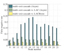
Fig. 7 shows the node performances of various configurations on the INRIA pedestrian data set. Similar results are obtained as in the face detection experiment: again, our new boosting algorithms significantly outperform AdaBoost [6], AsymBoost [7], and are considerably better than Wu et al.’s post-processing methods [2] at most nodes. Compared with the face detection experiment, we obtain more obvious improvement on detecting pedestrians. This may be because pedestrian detection is much more difficult and there is more room for improving the detection performance.

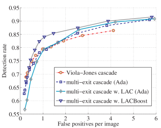
We have also compared the ROC curves of complete cascades, which are plotted in Fig. 8. FisherBoost and LACBoost perform better than all other compared methods. In contrast to the results of the detection rate for each node, LACBoost is slightly worse than FisherBoost in some cases (also see Fig. 9). In general, LAC and LDA post-processing improve those without post-processing. Also we can see that LAC post-processing performs slightly worse than other methods at the low false positive part. Probably LAC post-processing over-fits the training data in this case. Also, in the same condition, FisherBoost/LDA post-processing seems to perform better than LACBoost/LAC post-processing. We will discuss this issue in the next section.

Figure 9: Comparison between FisherBoost, LACBoost, HOG with the linear SVM of Dalal and Triggs [29], and Pyramid HOG with the histogram intersection kernel SVM (IKSVM) of Maji et al. [18]. In detection rate, our FisherBoost improves Dalal and Triggs’ approach by over $7\%$ at FPPI of $0.3$ on INRIA’s pedestrian detection dataset.

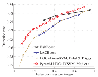
In summary, FisherBoost or LACBoost has superior performance than all the other algorithms. We have also compared FisherBoost and LACBoost with HOG with linear SVM of Dalal and Triggs [29], and the state-of-the-art on pedestrian detection—the pyramid HOG (PHOG) with histogram intersection kernel SVM (IKSVM) [18]. We keep all experiment configurations the same, except that HOG with linear SVM and PHOG with IKSVM have employed sophisticated mean shift to merge overlapped detection windows, while ours use the simple heuristic of Viola and Jones [6]. The results are reported in Fig. 9 and the observations are:

1. LACBoost performs similarly to Dalal and Triggs’ [29];

2. PHOG with nonlinear IKSVM performs much better than Dalal and Triggs’ HOG with linear SVM. This is consistent with the results reported in [18];

3. FisherBoost performs better than PHOG with IKSVM at the low FPPI part (lower than $0.5$).

Note that our FisherBoost and LACBoost use HOG, instead of PHOG. It is not clear how much gain PHOG has contributed to the final detection performance in the case of PHOG plus IKSVM of [18].

In terms of efficiency in the test phase for each method, our FisherBoost or LACBoost needs about $0.7$ seconds on average on the INRIA test data (no image re-scaling is applied and single CPU core is used on our workstation). PHOG with IKSVM needs about $8.3$ seconds on average. So our boosting framework is about $14$ times faster than PHOG with IKSVM. Note that HOG with linear SVM is much slower ($50$ to $70$ times slower than the boosting framework), which agrees with the results in [47].

In both face and pedestrian detection experiments, we have observed that FisherBoost performs slightly better than LACBoost. We try to elaborate this on the following.

5.4 Why LDA Works Better Than LAC

Wu et al. observed that in many cases, LDA post-processing gives better detection rates on MIT+CMU face data than LAC [2]. When using the LDA criterion to select Haar features, Shen et al. [46] tried different combinations of the two classes’ covariance matrices for calculating the within-class matrix: $\mathbf{C}_{w}={\boldsymbol{\Sigma}}_{1}+\gamma{\boldsymbol{\Sigma}}_{2}$ with $\gamma$ a nonnegative constant. It is easy to see that $\gamma=1$ and $\gamma=0$ correspond to LDA and LAC, respectively. They found that setting $\gamma\in[0.5,1]$ gives best results on the MIT+CMU face detection task [46, 11].

According to the analysis in this work, LAC is optimal if the distribution of $[h_{1}(\mathbf{x}),h_{2}(\mathbf{x}),\cdots,h_{n}(\mathbf{x})]$ on the negative data is symmetric. In practice, this requirement may not be perfectly satisfied, especially for the first several node classifiers. At the same time, these early nodes have much more impact on the final cascade’s detection performance than other nodes. This may explain why in some cases the improvement of LAC is not significant. However, this does not explain why LDA (FisherBoost) works; and sometimes it is even better than LAC (LACBoost). At the first glance, LDA (or FisherBoost) by no means explicitly considers the imbalanced node learning objective. Wu et al. did not have a plausible explanation either [2, 1].

Proposition 5.1.

For object detection problems, the Fisher linear discriminant analysis can be viewed as a regularized version of linear asymmetric classification. In other words, linear discriminant analysis has already considered the asymmetric learning objective.

Proof:

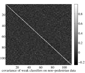
For object detection such as face and pedestrian detection considered here, the covariance matrix of the negative class is close to a scaled identity matrix. In theory, the negative data can be anything other than the target. Let us look at one of the off-diagonal elements

$${\boldsymbol{\Sigma}}_{ij,i\neq j} ={\mathbb{E}}[(h_{i}(\mathbf{x})-{\mathbb{E}}[h_{i}(\mathbf{x})])(h_{j}(\mathbf{x})-{\mathbb{E}}[h_{j}(\mathbf{x})])]$$

$$={\mathbb{E}}[h_{i}(\mathbf{x})h_{j}(\mathbf{x})]\approx 0.$$ (36)

Here $\mathbf{x}$ is the image feature of the negative class. We can assume that $\mathbf{x}$ is i.i.d. and approximately, $\mathbf{x}$ follows a uniform distribution. So ${\mathbb{E}}[h_{i,j}(\mathbf{x})]=0$. That is to say, on the negative class, the chance of $h_{i,j}(\mathbf{x})=+1$ or $h_{i,j}(\mathbf{x})=-1$ is the same, which is $50\%$. Note that this does not apply to the positive class because $\mathbf{x}$ of the positive class is not uniformly distributed. The last equality of (36) uses the fact that weak classifiers $h_{i}(\cdot)$ and $h_{j}(\cdot)$ are approximately statistically independent. Although this assumption may not hold in practice as pointed out in [41], it could be a plausible approximation.

Therefore, the off-diagonal elements of ${\boldsymbol{\Sigma}}$ are almost all zeros; and ${\boldsymbol{\Sigma}}$ is a diagonal matrix. Moreover in object detection, it is a reasonable assumption that the diagonal elements ${\mathbb{E}}[h_{j}(\mathbf{x})h_{j}(\mathbf{x})]$ $(j=1,2,\cdots)$ have similar values. Hence, ${\boldsymbol{\Sigma}}_{2}\approx v\bf I$ holds, with $v$ a positive constant.

So for object detection, the only difference between LAC and LDA is that, for LAC $\mathbf{C}_{w}=\frac{m_{1}}{m}{\boldsymbol{\Sigma}}_{1}$ and for LDA $\mathbf{C}_{w}=\frac{m_{1}}{m}{\boldsymbol{\Sigma}}_{1}+v\cdot\frac{m_{2}}{m}\bf I$. This concludes the proof. ∎

It seems that this regularization term can be the reason why the LDA post-processing approach and FisherBoost works even better than LAC and LACBoost in object detection. However, in practice, the negative data are not necessarily uniformly distributed. Particularly, in latter nodes, bootstrapping makes negative data to be those difficult ones. In this case, it may deteriorate the performance by completely ignoring the negative data’s covariance information.

In FisherBoost, this regularization is equivalent to have a $\ell_{2}$ norm regularization on the primal variable $\mathbf{w}$, $\|\mathbf{w}\|_{2}^{2}$, in the objective function of the QP problem in Section 4. Machine learning algorithms like Ridge regression use $\ell_{2}$ norm regularization.

Fig. 10 shows some empirical evidence that ${\boldsymbol{\Sigma}}_{2}$ is close to a scaled identity matrix. As we can see, the diagonal elements are much larger than those off-diagonal elements (off-diagonal ones are close to zeros).

Figure 10: The covariance matrix of the first $112$ weak classifiers selected by FisherBoost on non-pedestrian data. It may be approximated by a scaled identity matrix. On average, the magnitude of diagonal elements is $20$ times larger than those off-diagonal elements.

6 Conclusion

By explicitly taking into account the node learning goal in cascade classifiers, we have designed new boosting algorithms for more effective object detection. Experiments validate the superiority of the methods developed, which we have labeled FisherBoost and LACBoost. We have also proposed the use of entropic gradient descent to efficiently implement FisherBoost and LACBoost. The proposed algorithms are easy to implement and can be applied to other asymmetric classification tasks in computer vision. We aim in future to design new asymmetric boosting algorithms by exploiting asymmetric kernel classification methods such as [51]. Compared with stage-wise AdaBoost, which is parameter-free, our boosting algorithms need to tune a parameter. We are also interested in developing parameter-free stage-wise boosting that considers the node learning objective.

Chunhua Shen obtained a Ph.D. degree in Computer Vision from University of Adelaide, Australia in 2006, an M.Phil. degree in Applied Statistics from Australian National University in 2009, an M.Sc. degree and a Bachelor in 2002 and 1999 respectively, both from Nanjing University, Nanjing, China. Since Oct. 2005, he has been working with the computer vision program, NICTA (National ICT Australia), Canberra Research Laboratory, where he is currently a senior researcher. His main research interests include statistical machine learning and computer vision. His recent research focuses on boosting algorithms and their applications in real-time object detection. He has published over $50$ peer-reviewed papers in international conferences and journals.

Peng Wang is currently pursuing his Ph.D. degree at the School of Automation Science and Electrical Engineering, Beihang University, Beijing, China. He received the B.Sc degree from Beihang University in 2004. His research interests include machine learning and computer vision. From Sept. 2008 to Sept. 2010, he was a visiting scholar at NICTA, Canberra Research Laboratory, Canberra, Australia.

Anton van den Hengel is the founding director of The Australian Center for Visual Technologies (ACVT), an interdisciplinary research center focusing on innovation and education in the production and analysis of visual digital media. Prof. van den Hengel received a Ph.D. in Computer Vision in 2000, a Masters degree in Computer Science in 1994, a Bachelor of Law in 1993, and a Bachelor of Mathematical Science in 1991, all from The University of Adelaide. Prof. van den Hengel won the CVPR Best Paper Award in 2010.

References

- [1] J. Wu, M. D. Mullin, and J. M. Rehg, “Linear asymmetric classifier for cascade detectors,” in Proc. Int. Conf. Mach. Learn., Bonn, Germany, 2005, pp. 988–995.
- [2] J. Wu, S. C. Brubaker, M. D. Mullin, and J. M. Rehg, “Fast asymmetric learning for cascade face detection,” IEEE Trans. Pattern Anal. Mach. Intell., vol. 30, no. 3, pp. 369–382, 2008.
- [3] S. C. Brubaker, J. Wu, J. Sun, M. D. Mullin, and J. M. Rehg, “On the design of cascades of boosted ensembles for face detection,” Int. J. Comp. Vis., vol. 77, no. 1–3, pp. 65–86, 2008.
- [4] J. Bi, S. Periaswamy, K. Okada, T. Kubota, G. Fung, M. Salganicoff, and R. B. Rao, “Computer aided detection via asymmetric cascade of sparse hyperplane classifiers,” in Proc. ACM Int. Conf. Knowledge Discovery & Data Mining, Philadelphia, PA, USA, 2006, pp. 837–844.
- [5] M. Dundar and J. Bi, “Joint optimization of cascaded classifiers for computer aided detection,” in Proc. IEEE Conf. Comp. Vis. Patt. Recogn., Minneapolis, MN, USA, 2007.
- [6] P. Viola and M. J. Jones, “Robust real-time face detection,” Int. J. Comp. Vis., vol. 57, no. 2, pp. 137–154, 2004.
- [7] P. Viola and M. Jones, “Fast and robust classification using asymmetric AdaBoost and a detector cascade,” in Proc. Adv. Neural Inf. Process. Syst. 2002, pp. 1311–1318, MIT Press.
- [8] M.-T. Pham and T.-J. Cham, “Online learning asymmetric boosted classifiers for object detection,” in Proc. IEEE Conf. Comp. Vis. Patt. Recogn., Minneapolis, MN, 2007.
- [9] M.-T. Pham, V.-D. D. Hoang, and T.-J. Cham, “Detection with multi-exit asymmetric boosting,” in Proc. IEEE Conf. Comp. Vis. Patt. Recogn., Anchorage, Alaska, 2008.
- [10] S. Z. Li and Z. Zhang, “FloatBoost learning and statistical face detection,” IEEE Trans. Pattern Anal. Mach. Intell., vol. 26, no. 9, pp. 1112–1123, 2004.
- [11] S. Paisitkriangkrai, C. Shen, and J. Zhang, “Efficiently training a better visual detector with sparse Eigenvectors,” in Proc. IEEE Conf. Comp. Vis. Patt. Recogn., Miami, Florida, US, June 2009.
- [12] C. Shen, S. Paisitkriangkrai, and J. Zhang, “Face detection from few training examples,” in Proc. Int. Conf. Image Process., San Diego, California, USA, 2008, pp. 2764–2767.
- [13] S. Paisitkriangkrai, C. Shen, and J. Zhang, “Fast pedestrian detection using a cascade of boosted covariance features,” IEEE Trans. Circuits Syst. Video Technol., vol. 18, no. 8, pp. 1140–1151, 2008.
- [14] P. Wang, C. Shen, N. Barnes, H. Zheng, and Z. Ren, “Asymmetric totally-corrective boosting for real-time object detection,” in Proc. Asian Conf. Comp. Vis., Queenstown, New Zealand, 2010.
- [15] H. Masnadi-Shirazi and N. Vasconcelos, “Asymmetric boosting,” in Proc. Int. Conf. Mach. Learn., Corvalis, Oregon, US, 2007, pp. 609–619.
- [16] C. Shen, P. Wang, and H. Li, “LACBoost and FisherBoost: Optimally building cascade classifiers,” in Proc. Eur. Conf. Comp. Vis., Crete Island, Greece, 2010, vol. 2, LNCS 6312, pp. 608–621.
- [17] A. Demiriz, K.P. Bennett, and J. Shawe-Taylor, “Linear programming boosting via column generation,” Mach. Learn., vol. 46, no. 1-3, pp. 225–254, 2002.
- [18] S. Maji, A. C. Berg, and J. Malik, “Classification using intersection kernel support vector machines is efficient,” in Proc. IEEE Conf. Comp. Vis. Patt. Recogn., Anchorage, AK, US, 2008.
- [19] L. Bourdev and J. Brandt, “Robust object detection via soft cascade,” in Proc. IEEE Conf. Comp. Vis. Patt. Recogn., San Diego, CA, US, 2005, pp. 236–243.
- [20] R. Xiao, H. Zhu, H. Sun, and X. Tang, “Dynamic cascades for face detection,” in Proc. IEEE Int. Conf. Comp. Vis., Rio de Janeiro, Brazil, 2007.
- [21] J. Wu, J. M. Rehg, and M. D. Mullin, “Learning a rare event detection cascade by direct feature selection,” in Proc. Adv. Neural Inf. Process. Syst., S. Thrun, L. Saul, and B. Schölkopf, Eds., 2003.
- [22] M.-T. Pham and T.-J. Cham, “Fast training and selection of Haar features using statistics in boosting-based face detection,” in Proc. IEEE Int. Conf. Comp. Vis., Rio de Janeiro, Brazil, 2007.
- [23] C. Liu and H.-Y. Shum, “Kullback-Leibler boosting,” in Proc. IEEE Conf. Comp. Vis. Patt. Recogn., Madison, Wisconsin, June 2003, vol. 1, pp. 587–594.
- [24] O. Tuzel, F. Porikli, and P. Meer, “Pedestrian detection via classification on Riemannian manifolds,” IEEE Trans. Pattern Anal. Mach. Intell., vol. 30, no. 10, pp. 1713–1727, 2008.
- [25] A. Torralba, K. P. Murphy, and W. T. Freeman, “Sharing visual features for multiclass and multiview object detection,” IEEE Trans. Pattern Anal. Mach. Intell., vol. 29, no. 5, pp. 854–869, 2007.
- [26] P. Viola, J. C. Platt, and C. Zhang, “Multiple instance boosting for object detection,” in Proc. Adv. Neural Inf. Process. Syst., Vancouver, Canada, 2005, pp. 1417–1424.
- [27] P. Dollár, B. Babenko, S. Belongie, P. Perona, and Z. Tu, “Multiple component learning for object detection,” in Proc. Eur. Conf. Comp. Vis., Marseille, France, 2008, pp. 211–224.
- [28] Z. Lin, G. Hua, and L. S. Davis, “Multiple instance feature for robust part-based object detection,” in Proc. IEEE Conf. Comp. Vis. Patt. Recogn., Miami, FL, US, 2009, pp. 405–412.
- [29] N. Dalal and B. Triggs, “Histograms of oriented gradients for human detection,” in Proc. IEEE Conf. Comp. Vis. Patt. Recogn., San Diego, CA, 2005, vol. 1, pp. 886–893.
- [30] D. Aldavert, A. Ramisa, R. Toledo, and R. Lopez de Mantaras, “Fast and robust object segmentation with the integral linear classifier,” in Proc. IEEE Conf. Comp. Vis. Patt. Recogn., San Francisco, US, 2010.
- [31] W. Wang, J. Zhang, and C. Shen, “Improved human detection and classification in thermal images,” in Proc. Int. Conf. Image Process., Hong Kong, 2010.
- [32] Y. Mu, S. Yan, Y. Liu, T. Huang, and B. Zhou, “Discriminative local binary patterns for human detection in personal album,” in Proc. IEEE Conf. Comp. Vis. Patt. Recogn., Anchorage, AK, US, 2008.
- [33] Y. Zheng, C. Shen, and X. Huang, “Pedestrian detection using center-symmetric local binary patterns,” in Proc. Int. Conf. Image Process., Hong Kong, 2010.
- [34] X. Wang, T. X. Han, and S. Yan, “An HOG-LBP human detector with partial occlusion handling,” in Proc. IEEE Int. Conf. Comp. Vis., Rio de Janeiro, Brazil, 2007.
- [35] B. Wu and R. Nevatia, “Optimizing discrimination-efficiency tradeoff in integrating heterogeneous local features for object detection,” in Proc. IEEE Conf. Comp. Vis. Patt. Recogn., Anchorage, AK, US, 2008.
- [36] M. Enzweiler, A. Eigenstetter, B. Schiele, and D. M. Gavrila, “Multi-cue pedestrian classification with partial occlusion handling,” in Proc. IEEE Conf. Comp. Vis. Patt. Recogn., San Francisco, US, 2010.
- [37] G. R. G. Lanckriet, L. El Ghaoui, C. Bhattacharyya, and M. I. Jordan, “A robust minimax approach to classification,” J. Mach. Learn. Res., vol. 3, pp. 555–582, Dec. 2002.
- [38] S. Boyd and L. Vandenberghe, Convex Optimization, Cambridge University Press, 2004.
- [39] Y.-L. Yu, Y. Li, D. Schuurmans, and C. Szepesvári, “A general projection property for distribution families,” in Proc. Adv. Neural Inf. Process. Syst., Y. Bengio, D. Schuurmans, J. Lafferty, C. K. I. Williams, and A. Culotta, Eds., Vancouver, Canada, 2009, pp. 2232–2240.
- [40] K. Huang, H. Yang, I. King, M. Lyu, and L. Chan, “The minimum error minimax probability machine,” J. Mach. Learn. Res., vol. 5, pp. 1253–1286, Dec. 2004.
- [41] C. Shen and H. Li, “On the dual formulation of boosting algorithms,” IEEE Trans. Pattern Anal. Mach. Intell., 25 Feb. 2010, IEEE computer Society Digital Library. http://dx.doi.org/10.1109/TPAMI.2010.47 .
- [42] G. Rätsch, S. Mika, B. Schölkopf, and K.-R. Müller, “Constructing boosting algorithms from SVMs: An application to one-class classification,” IEEE Trans. Pattern Anal. Mach. Intell., vol. 24, no. 9, pp. 1184–1199, 2002.
- [43] A. Beck and M. Teboulle, “Mirror descent and nonlinear projected subgradient methods for convex optimization,” Oper. Res. Lett., vol. 31, no. 3, pp. 167–175, 2003.
- [44] M. Collins, A. Globerson, T. Koo, X. Carreras, and P. L. Bartlett, “Exponentiated gradient algorithms for conditional random fields and max-margin Markov networks,” J. Mach. Learn. Res., pp. 1775–1822, 2008.
- [45] MOSEK ApS, “The MOSEK optimization toolbox for matlab manual, version 5.0, revision 93,” 2008, http://www.mosek.com/.
- [46] C. Shen, S. Paisitkriangkrai, and J. Zhang, “Efficiently learning a detection cascade with sparse Eigenvectors,” IEEE Trans. Image Process., 1 July 2010, http://dx.doi.org/10.1109/TIP.2010.2055880.
- [47] Q. Zhu, S. Avidan, M.-C. Yeh, and K.-T. Cheng, “Fast human detection using a cascade of histograms of oriented gradients,” in Proc. IEEE Conf. Comp. Vis. Patt. Recogn., New York City, USA, 2006, pp. 1491–1498.
- [48] M. Everingham, L. van Gool, C. Williams, J. Winn, and A. Zisserman, “The Pascal visual object classes (VOC) challenge,” Int. J. Comp. Vis., vol. 88, no. 2, pp. 303–338, 2010.
- [49] P. Dollár, C. Wojek, B. Schiele, and P. Perona, “Pedestrian detection: A benchmark,” in Proc. IEEE Conf. Comp. Vis. Patt. Recogn., Miami, FL, US, 2009, pp. 304–311.
- [50] A. Bosch, A. Zisserman, and X. Munoz, “Representing shape with a spatial pyramid kernel,” in Proc. ACM Int. Conf. Image Video Retrieval, Amsterdam, The Netherlands, 2007, pp. 401–408.
- [51] H.-H. Tu and H.-T. Lin, “One-sided support vector regression for multiclass cost-sensitive classification,” in Proc. Int. Conf. Mach. Learn., Haifa, Israel, 2010.
![[Uncaptioned image]](/html/1008.3742/assets/Figs/Shen.png) |