Stimulation of the fluctuation superconductivity by the $\mathcal{PT}$-symmetry

Abstract

We discuss fluctuations near the second order phase transition where the free energy has an additional non-Hermitian term. The spectrum of the fluctuations changes when the odd-parity potential amplitude exceeds the critical value corresponding to the $\mathcal{PT}$-symmetry breakdown in the topological structure of the Hilbert space of the effective non-Hermitian Hamiltonian. We calculate the fluctuation contribution to the differential resistance of a superconducting weak link and find the manifestation of the $\mathcal{PT}$-symmetry breaking in its temperature evolution. We successfully validate our theory by carrying out measurements of far from equilibrium transport in mesoscale-patterned superconducting wires.

An Hermitian character of the Hamiltonian expressed by the condition $H^{\dagger}=H$ is a cornerstone of quantum mechanics as it ensures that the energies of its stationary states are real. Yet it was discovered not long ago Bender1 that the weaker requirement $H^{\ddagger}=H$, where ${\ddagger}$ represents combined parity reflection and time reversal (${\cal PT}$), introduces new classes of complex Hamiltonians Feshbach whose spectra are still real and positive Bender1 ; Bender2 ; Roy ; Uwe . This generalization of Hermiticity opened a new field of research in quantum mechanics and beyond that had been enjoying ever since a rapid growth.

We focus here on the superconducting fluctuations above the superconductor – normal metal transition in quasi 1D superconducting wire of the finite length $L$ driven far from equilibrium by an electric field $\mathcal{E}$, see Fig. 1. We show that either the presence or absence of ${\cal PT}$-symmetry in the Cooperon (fluctuation) propagator, which depends on the magnitude of $\mathcal{E}$, effects strongly the structure of fluctuations.

The $\mathcal{PT}$-symmetrical state corresponds to small drive, $|\mathcal{E}|<\mathcal{E}_{c}$, where $\mathcal{E}_{c}$ is of the order of the Thouless energy, $E_{\rm Th}=\hbar D/L^{2}$, the characteristic energy scale of the dirty quasi-one-dimensional conductor, see Fig. 1, where $D$ is the electron diffusion coefficient in the wire and $L$ is its length. This state is nonequilibrium but stationary where fluctuating Cooper pairs survive in the presence of the electric field. Breaking the $\mathcal{PT}$-symmetry at $|\mathcal{E}|=\mathcal{E}_{c}$ is the dynamic phase transition from the stationary to the nonstationary dynamic state where the electric field quickly destroys the Cooper-pairs. In this state Cooper pair wave function qualitatively is represented as a linear superposition of the Ivlev-Kopnin “kinks” located at the wire ends Kopnin , having the phases that rotate with the opposite rate. We calculate the fluctuation correction to conductivity and show that for $|\mathcal{E}|>\mathcal{E}_{c}$ this correction is strongly suppressed by an electric field. It implies that $\mathcal{PT}$-symmetry effectively protects Cooper pairs from the detrimental effect of the electric field and stabilizes superconductivity.

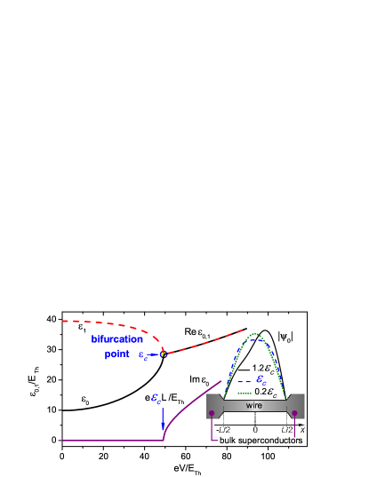
Figure 1: (Color online) Evolution of the two lowest energy levels, $\varepsilon_{0}$ and $\varepsilon_{1}$ upon applying bias $V={\mathcal{E}}L$. At $\mathcal{E}=\mathcal{E}_{c}$ the levels merge and form the complex conjugate pair at $\mathcal{E}>\mathcal{E}_{c}$. The inset shows the change of the eigenfunction $|\psi_{0}(x)|$, normalized to unity, upon variation of $\mathcal{E}$: $\psi_{0}(x)$ is symmetrical for $\mathcal{E}\leq\mathcal{E}_{c}$ and is asymmetric at $\mathcal{E}>\mathcal{E}_{c}$. The asymmetry of $\psi_{0}(x)$ is the signature of the $\mathcal{PT}$-invariance breakdown.

The dynamics of the superconducting fluctuations is described by the retarded fluctuation propagator $\hat{L}_{R}(t,t^{\prime};x,x^{\prime})$ Varlamov_book ; chtch :

$$\hat{L}_{R}^{-1}=\partial_{\rm t}+{\mathcal{H}}_{\rm eff}\,,$$ (1)

where we use the units $k_{\mathrm{B}}=e=\hbar=1$. The effective Hamiltonian, $\mathcal{H}_{\rm eff}[\mathcal{E}]$, describes the linearized Ginsburg-Landau (GL) field theory GL ; Kopninbook . In general, $\hat{L}_{R}$ can be expanded through the eigen functions $\psi_{n}$ and the eigen values $\varepsilon_{n}$ of ${\mathcal{H}}_{\rm eff}$:

$$\hat{L}_{R}(\omega;x,x^{\prime})=\sum_{n}\frac{\psi_{n}(x)\psi_{n}^{*}(x^{\prime})}{2i\omega-\varepsilon_{n}}.$$ (2)

We show below using the technique developed in Refs. Bender1 ; Uwe ; Kopnin that $\mathcal{PT}$-symmetry of $\hat{L}_{R}$ holds at low drives. At large $\mathcal{E}$ exceeding the certain critical value, $\mathcal{E}_{c}$, the $\mathcal{PT}$-invariance breaks down and the two lowest energy states $\varepsilon_{0}$ and $\varepsilon_{1}$ of $H_{\rm eff}$ merge. At $\mathcal{E}>\mathcal{E}_{c}$ they form the complex conjugate pair (Fig.1). From the general viewpoint of the catastrophe theory Arnold bifurcations of $H_{\rm eff}[\mathcal{E}]$ belong to the so-called fold catastrophe topological class. This class of the bifurcations is (topologically) protected with respect to small local perturbation of ${\mathcal{H}}_{\rm eff}$ preserving the symmetry of the system. Therefore, in order to establish the existence of the bifurcation and to find its type it would suffice to investigate the effective Hamiltonian, $\mathcal{H}_{\rm eff}=-D\nabla_{x}^{2}-\tau^{-1}-2i\varphi$. Here $\varphi$ is the potential of the electric field responsible for the nonhermitivity of $\mathcal{H}_{\rm eff}$. In application to our problem, neglecting in $\mathcal{H}_{\rm eff}$ the decay of the mean-field superconducting order parameter from the reservoirs into the wire does not violate the catastrophe theory classification of bifurcation symmetries. For the same reason one may choose the boundary conditions in a form: $\psi(x=\pm L/2\mp 0)=\psi(x\to\pm\infty)=0$. Here $\tau$ is the GL-time and $D>0$ is the material constant (e.g., electron diffusion coefficient in the dirty superconductor). We further discuss the case where $\varphi(x)=\mathcal{E}x$ and $x$ is the coordinate along the wire.

The problem

$${\cal{H}}_{\rm eff}\psi=\varepsilon\psi,$$ (3)

can be solved using the anzatz Kopnin :

$$\psi(x)=\alpha\operatorname{Ai}(Z)+\beta\operatorname{Bi}(Z),$$ (4)

$$Z(x)=\frac{\varepsilon+2ix\mathcal{E}}{E_{\mathrm{Th}}}\left(\frac{E_{\mathrm{Th}}}{2V}\right)^{2/3}\,,$$ (5)

where $\operatorname{Ai}$ and $\operatorname{Bi}$ are the Airy-functions, and $\alpha$, $\beta$ are fixed by the boundary conditions. We absorbed $\tau^{-1}$ into the definition of $\varepsilon$. Then the equation determining the eigenvalues acquires the form:

$$F(\varepsilon,\mathcal{E})\equiv\operatorname{Im}\left[\operatorname{Ai}(Z(L/2))\operatorname{Bi}(Z(-L/2))\right]=0.$$ (6)

The critical field $\mathcal{E}_{c}$ is the field of emergence of the first bifurcation Trenogin ; Arnold of Eq.(6) corresponding to merging of lowest levels and is given by the conditions

$$F(\varepsilon_{c},\mathcal{E}_{c})=0\,,\,\,\,\,\,\,\,\partial_{\varepsilon}F(\varepsilon_{c},\mathcal{E}_{c})=0\,,$$ (7)

where $\varepsilon_{c}$ is the value of the energy at the levels merging point. We find $\mathcal{E}_{c}\approx 49.25E_{\mathrm{Th}}/L$, where $\varepsilon_{c}=\varepsilon_{0}=\varepsilon_{1}\approx 28.43E_{\mathrm{Th}}$. The same conditions give the next bifurcations where higher pairs of levels merge pairwise, $\mathcal{E}_{c}^{(1)}\approx 4\mathcal{E_{\rm c}}$, $\mathcal{E}_{c}^{(2)}\approx 10\mathcal{E_{\rm c}}$, etc… As we have mentioned above, the bifurcations described here belong to the universality class of the “fold catastrophe” ($A_{2}$ in ADE classification). Then $\mathcal{E}_{c}$ is the tipping point of the catastrophe.

Expanding Eq.(6) near the bifurcation one finds $[\frac{1}{2}(\varepsilon-\varepsilon_{c})^{2}\partial^{2}_{\varepsilon}+(\mathcal{E}-\mathcal{E}_{c})\partial_{\mathcal{E}_{c}}]F(\varepsilon,\mathcal{E})|_{\varepsilon\to\varepsilon_{c},\mathcal{E}\to\mathcal{E}_{c}}=0$, so,

$$\varepsilon_{0,1}(\mathcal{E})\approx\varepsilon_{c}\mp E_{\mathrm{Th}}\sqrt{\eta\left[1-\frac{\mathcal{E}^{2}}{\mathcal{E}_{c}^{2}}\right]},$$ (8)

$$\eta=\mathcal{E}_{c}\frac{\partial_{\mathcal{E}_{c}}F(\varepsilon_{c},\mathcal{E}_{c})}{E_{\mathrm{Th}}^{2}\partial^{2}_{\varepsilon}F(\varepsilon_{c},\mathcal{E}_{c})}\approx\frac{\pi^{2}}{\sqrt{2}}\frac{L{\mathcal{E}_{c}}}{{E_{\mathrm{Th}}}}.$$

The results of the numerical solution of the eigenvalue problem are shown in Fig.1 note . In the limiting case of the semi-infinite wire, $\psi_{0,1}$ for $\mathcal{E}>\mathcal{E}_{c}$ change with coordinates similarly to the solution for the order parameter found in Ref. Kopnin .

Now we proceed with the analysis of the dynamics of the fluctuations in the wire using the following equation:

$$(\hat{L}^{R})^{-1}\psi=0.$$ (9)

As long as the field does not exceed the critical value, $\mathcal{E}<\mathcal{E}_{c}$, the stationary solution of Eq.(1) remains stable and is given by

$$\psi(x)\simeq\psi_{0}(x),$$ (10)

where we have taken $\tau^{-1}=\varepsilon_{0}$. This solution is $\mathcal{PT}$-invariant, i.e. $|\psi_{0}(x)|=|\psi_{0}(-x)|$, see Fig.1. The extremum of $|\psi_{0}(x)|$ is thus located at $x=0$, at the center of the weak link. The effective field-dependent critical temperature for the superfluid correlations-induced superfluidity within the weak link is to be found from the relation $\tau^{-1}=\varepsilon_{0}$ and is given by $T_{c}^{\rm(eff)}(\mathcal{E})=T_{c}-\pi\varepsilon_{0}(\mathcal{E})/8$. The $T_{c}^{\rm(eff)}(\mathcal{E})$ dependence become singular near the critical field $\mathcal{E}_{c}$, ${dT_{c}^{\rm(eff)}}/{d\mathcal{E}}|_{{\mathcal{E}}={\mathcal{E}_{c}}}=\infty$; this singularity results in the anomalous behaviour of the nonlinear fluctuation corrections to the conductivity. As the field goes above the threshold, $\mathcal{E}>\mathcal{E}_{c}$, the stationary solution of Eq.(1) ceases to exist. The eigenvalues become complex conjugate, $\operatorname{Re}\varepsilon_{0}=-\operatorname{Re}\varepsilon_{1}=\tau^{-1}$ [see inset in Fig.1], and

$$\operatorname{Im}\varepsilon_{0}(\mathcal{E})=-\operatorname{Im}\varepsilon_{1}(\mathcal{E})\approx E_{\mathrm{Th}}\sqrt{\eta\left[\frac{\mathcal{E}^{2}}{\mathcal{E}_{c}^{2}}-1\right]}.$$ (11)

The eigenfunctions at $\mathcal{E}>\mathcal{E}_{c}$ are not $\mathcal{PT}$-invariant any more, $|\psi_{i}(x)|\neq|\psi_{i}(-x)|$, $i=1,2$. Thus

$$\psi\sim e^{-i\operatorname{Im}(\varepsilon_{0}-\varepsilon_{1})t/2}\psi_{0}(x)+e^{i\operatorname{Im}(\varepsilon_{0}-\varepsilon_{1})t/2}\psi_{1}(x).$$ (12)

This implies that the order parameter becomes two-component with the relative phase between the two components rotating with the Josephson frequency $\operatorname{Im}(\varepsilon_{0}-\varepsilon_{1})$. Since $|\psi_{0}(x)|=|\psi_{1}(-x)|$, the time averaged order parameter $\langle|\psi(x)|^{2}\rangle_{\rm time}\sim|\psi_{0}(x)|^{2}+|\psi_{0}(-x)|^{2}$ and develops a dip at $x=0$, increasing in amplitude with growing $\mathcal{E}$. This spot of the relatively suppressed superfluidity finally serves as a heating nucleus in the weak link.

Having calculated the eigenvalues $\varepsilon_{n}$ and the eigenfunctions, $\psi_{n}$, $n=0,1,\ldots$, of ${\cal H}_{\rm eff}$, we proceed with the analysis of the superfluidity in the wire under the external drive. We will focus on the effect of superconducting fluctuations on the conductivity of the weak link. The most singular fluctuation contributions to the conductivity come from the Maki-Thompson and Aslamazov-Larkin mechanisms Varlamov_book ; chtch ; varlamov1992 , and the corresponding currents read

$$j^{\scriptscriptstyle{\rm(MT)}}=2DT^{2}\mathcal{E}\operatorname{Tr}\{(L^{R}_{\omega})^{\tau}(C^{R}_{\varepsilon})^{\tau}C^{A}_{\varepsilon}L^{A}_{\omega}\}\partial_{\epsilon}n_{F}(\tilde{\epsilon}),$$ (13)

$$j^{\scriptscriptstyle{\rm(AL)}}=DT^{2}\operatorname{Tr}\{(L^{R}_{\omega})^{\tau}(C^{R}_{\varepsilon})^{\tau}\nabla C^{R}_{\varepsilon}L^{A}_{\omega}+h.c.\}\delta n\,,$$

where $T$ is the temperature, $\tilde{\epsilon}=\epsilon+\omega$, $\delta n=n_{F}(\tilde{\epsilon}+\varphi)-n_{F}(\tilde{\epsilon}-\varphi)$, $C^{R(A)}_{\varepsilon}=4[D\nabla_{\mathrm{x}}^{2}\pm 2i\varepsilon+\gamma]^{-1}$ is the retarded (advanced) Cooperon propagator, $\gamma$ is the inelastic relaxation rate, and trace ‘$\operatorname{Tr}$’ means the integration over coordinates, $\varepsilon$ and $\omega$ (the latter two with the weights $1/2\pi$). Writing Eq.(13) in terms of $L^{R(A)}$ and $C^{R(A)}$ eigenfunctions and eigenvalues yields the fluctuation correction to the resistance as (hereafter we restore the physical units and dimensions of the weak link)

$$\delta R\sim-\frac{E_{\rm Th}^{2}d}{e^{2}k_{\mathrm{B}}TL}\frac{1}{\sqrt{(\tau^{-1}-\operatorname{Re}\varepsilon_{0}(\mathcal{E})/\hbar)^{2}+(\Gamma(\mathcal{E})+\gamma)^{2}}}\,,$$ (14)

where $d$ is the weak link thickness, $\Gamma=\operatorname{Im}\varepsilon_{0}$ and $\tau^{-1}=8(T_{\rm c}-T)/\pi$ while $T_{\rm c}$ is the critical temperature in the bulk. The resistance displays a pronounced voltage dependence in the range of parameters where either $\hbar/\tau\sim\varepsilon_{0}(\cal E)$ or ${\cal E}\sim{\cal E}_{c}$. So, $\delta R(V)$ behaviour can be controlled via changing $\tau$ by cooling or heating the system.

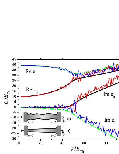
Figure 2: Evolution of the two lowest energy levels, $\varepsilon_{0}$ and $\varepsilon_{1}$ upon applying bias $V={\mathcal{E}}L$ when the wire is not $\mathcal{P}$-symmetric [so $\mathcal{PT}$-symmetry is also broken] due to the spatial variation of the wire thickness $d$ with $~{}5\%$ relative amplitude: a) $d$ fluctuates according to the gaussian law, $\varepsilon_{0}$ is the red curve and $\varepsilon_{1}$ is the blue one and b) the wire width monotonically changes, $\varepsilon_{0}$ is the black curve and $\varepsilon_{1}$ is the green one. In both cases the bifurcation is smoothed and the energies become complex below $\mathcal{E}_{c}$. So $\Gamma>0$ and as the result we get the suppression of the fluctuational Cooper pair contributions to the conductivity compared to the case of the $\mathcal{P}$-symmetric wire, see Fig. 1.

The regime $|\mathcal{E}|<\mathcal{E}_{c}$ when the system is $\mathcal{PT}$-symmetric favors fluctuational Cooper pairs. When $|\mathcal{E}|>\mathcal{E}_{c}$ the spectrum of fluctuation propagator becomes complex that implies breaking of the Cooper pairs by the electric field with the rate $\tilde{\Gamma}\neq 0$ that increases with the increase of $\mathcal{E}$. It follows from Eqs. (13) and Eq. (14) that then the correction to the resistance from the fluctuating Cooper pairs quickly switches off. The same conclusion follows from the investigation of the superconducting wire where the $\mathcal{P}$-symmetry is broken due to geometrical imperfection, see Fig. 2.

What we have investigated above was the behavior of the superconducting fluctuations within the framework of the quadratic Keldysh action describing the fluctuations of the order parameter, see Ref. chtch . The natural question that arises is whether the revealed bifurcation picture retains in case of large fluctuations where one has to go beyond the Gaussian approximation. We expect the affirmative answer since the predicted instability follows from the symmetry considerations analogous to those in the general theory of the second phase transitions which, as one can prove chtch , do not change upon appearance of the higher order terms. To cast the above reasoning into a mathematical form we note that on the heuristic level the large fluctuations would result in modifying (3) into the nonlinear, but having the same symmetry, Schrödinger equation. The corresponding generalization of Eq.(3) has the form:

$$\theta^{{}^{\prime\prime}}+2i(E+x\mathcal{E})\sin\theta=0\,,$$ (15)

The boundary conditions at $x=\pm L/2$ we take in a more general form: $\theta(0)=\theta_{s1}$ and $\theta(L)=\theta_{s2}$, where $\theta_{s1,2}$ are parameterized as follows: $\theta_{s1,2}(E)=\frac{1}{2}(\pi+i\ln\frac{\Delta+E\mp V/2}{\ \Delta-E\pm V/2})$, where $\Delta$ is constant. [For $\mathcal{E}=0$ Eq. (15) formally coincides with the Usadel equation minigap for the $\theta$ angle parameterizing the quasiclassical retarded Greens function in the superconducting weak link with the order parameter $\Delta$ in the reservoirs.]. Expanding $\sinh\theta$ and identifying $2iE$ with $\epsilon-\tau^{-1}$ and $\theta$ with $\psi$ one recovers Eq.(3). We solved Eq. (15) numerically and found that the first fold-bifurcation appears at $\mathcal{E}_{c}\approx 5E_{\mathrm{Th}}/L$ rather than $\approx 49E_{\mathrm{Th}}/L$ found in Eq.(3). We thus have demonstrated that even in case of large fluctuations, where the extension beyond the linear approximation is required, the bifurcation of the fluctuation spectrum preserves, while the value of the critical field $\mathcal{E}_{c}$ where it occurs may change.

We have focused here on the superconducting wire of relatively small length that generated us the characteristic energy scale $E_{\rm Th}$. Our solution for the $\mathcal{PT}$-symmetry breaking bifurcation and the fluctuations heavily relied on the discrete nature of $H_{\rm eff}$ spectrum. In the infinite geometry, $L\to\infty$, $E_{T}\to 0$, and the spectrum of $H_{\rm eff}$ is continuous. Then there is no $\mathcal{PT}$-symmetry breaking bifurcation. Taking the integral in Eq.(13) over the continues spectrum of $H_{\rm eff}$ we would get fluctuation corrections to the resistance with the form different from Eq. (14). Then the effective pair breaking electric field $\mathcal{E}_{c}\sim 1/\xi\tau$ varlamov1992 as follows from the uncertainty relation between $\tau$ and $\Gamma\sim\xi\mathcal{E}_{c}$, where $\xi=\sqrt{D\tau}$.

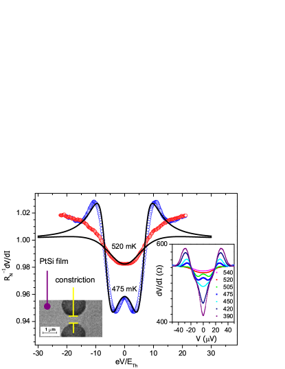
Figure 3: The differential resistance of the superconducting weak link. The left inset presents scanning electron microscope image of the experimentally studied system, the constriction made by the electron beam lithography out of the PtSi film of the thickness $d=6$ nm and having $T_{\mathrm{c}}=560$ mK. The details of the system preparation are given in SNS2 . The right inset displays the full set of the differential resistance vs. $V$ dependences at different temperatures given in mK in the legend. The central panel shows comparison of two exemplary experimental curves (symbols), normalized to $R_{\mathrm{N}}=536\,\Omega$, with the $dV/dI$ calculated from Eqs. (8) and (14) (solid lines). We took $L=0.4$ $\mu$m and $D=6$ cm${}^{2}/$s SNS2 , which gave $E_{\mathrm{Th}}=2.5\,\mu$eV, and chose $\hbar\Gamma/E_{\mathrm{Th}}=0.176$.

In order to test our theory we designed the experiments on mesoscale-patterned ultrathin PtSi wires having small constriction, as shown in Fig. 3. The details of the system preparation and parameters of the films are given in SNS2 and the Supplementary. The constriction plays the role of a weak link where fluctuation effects are expected to be very strong. The dimensions and the material characteristics were chosen to create the most favourable conditions for manifestation of the $\mathcal{PT}$-symmetry breaking effect in the system response to applied voltage bias. Namely, since the characteristiv energy scale, $E_{\mathrm{Th}}$, is inversely proportional to $L^{2}$, the length of the constriction should not be too large in order to diminish the disguising effect of the thermal broadening. Another restriction on $L$ is dictated by the condition that the characteristic drive $\mathcal{E}_{c}L$ remained less than superconducting gap. At the same time, in order to suppress Josephson coupling which could prevail over the fluctuation contribution, one has to take $L\gg\xi_{N}$, where $\xi_{N}=\sqrt{\hbar D/2\pi k_{B}T}$ is the decay length for the pair amplitude in diffusive normal conductor. Taking into account that, according to our calculations, the characteristic energy scale where fluctuations are important is about $10E_{Th}$, the above conditions imply that L should not be much larger than 10 $\xi_{N}$.

Figure 3 shows the differential resistance, $dV/dI$, of the superconducting weak link as function of the applied voltage bias, $V$. Upon cooling the system down from the critical temperature, the shape of the measured $dV/dI$-$V$ dependencies near $V=0$, transforms from the convex one, with the shallow minimum, into the $W$-shaped curve with a peak at $V=0$. With further decreasing temperature, the central knob inverts, and $dV/dI(V)$ acquires a pronounced progressively deepening V-shape developing on top of shallow minimum. Importantly, the width of the deep remains equal to that of the maximum (see the curves corresponding to $T\leq 450$ mK in the right inset to Fig. 3). The solid lines in the main panel present the $dV/dI$ vs. $V$ dependences calculated according to Eqs. (8) and (14), with $\Gamma$ being the only fitting parameter. The fit traces perfectly traces the temperature evolution of $dV/dI(V)$, and, most strikingly, the $W$-shape at $T=475$ K in all its details, including maxima in $dV/dI$ at $|eV|\approx 10E_{\mathrm{Th}}$ and the central knob $5E_{\mathrm{Th}}$ wide.

The similar behaviour of differential resistivity, the evolution from the shallow minimum to maximum and then to the dip again with the decreasing temperature, was observed in Ref. SNS1 , where the quest for the theoretical explanation of this effect was formulated. Using the parameters given in Ref. SNS1 (see Fig. 2 there) we estimate $\xi_{N}=0.14\,\mu$m at $T=1$ K, the bridge length being 2.8 $\mu$m. Furthermore, the corresponding $E_{\rm{Th}}\simeq 1.4\mu$V, and one sees that the characteristic voltage of “saddled” shaped structure around zero bias in SNS1 is about 40$E_{\rm{Th}}$ in accord with our notion that the $dV/dI$ features develop on the voltage scale well exceeding Thouless energy.

As a final remark, we stress that the temperature evolution of $dV/dI$ shape results from the confluence of the voltage-dependent fluctuation conductivity, stemming from the Maki-Thompson and Aslamazov-Larkin mechanisms, and the low-voltage quadratic dispersion $[\varepsilon_{0}(V)=\varepsilon_{0}(0)+aV^{2}$, see Fig.1] of the ground state energy. Importantly, the width of the central knob/peak is $\approx 5E_{Th}$, in a contrast to the more narrow dip in the tunnelling conductivity Birge (the knob in $dV/dI$ corresponds to the groove in $dI/dV$), having the width of $|eV|\approx E_{\mathrm{Th}}$ reflecting the suppression of the electronic density of states by the proximity effect. The observed effect also differs from the zero-bias conductance peak in NS and SNS junctions at low temperatures Klapwijk originating from the phase-coherent Andreev reflection.

In conclusion, we have demonstrated that the $\mathcal{PT}$-symmetry favors fluctuating Cooper pairs in the superconducting weak link. We have found that the applied electric field exceeding the critical value, $\mathcal{E}_{c}$, breaks down the $\mathcal{PT}$-symmetry and destroys the superconducting fluctuations in the weak link and derived the expression for $\mathcal{E}_{c}$. Combining effects of superconducting fluctuations and the low-voltage dispersion of the ground state energy of the effective non-Hermitian Hamiltonian of the fluctuating Cooper pairs we have quantitatively described the experimentally observed differential resistance of the weak link in the vicinity of the critical temperature.

We thank N. Kopnin, A. Varlamov, A. Mal’tsev, A. Levchenko, and D. Vodolazov for helpful discussions. The work was funded by the U.S. Department of Energy Office of Science through the contract DE-AC02-06CH11357 and by Russian Foundation for Basic Research (Grants No. 10-02-00700 and 12-02-00152), and the Programs of the Russian Academy of Sciences.

Appendix A Supplementary material

A.1 The boundary conditions for GL-equations

Figure 4: The boundary with the normal resistance $R$ between the superconductors with the order parameters $\Delta_{1}$ and $\Delta_{2}$.

The boundary conditions for GL-equations Bcond on the surface between two superconductors (or a superconductor and a normal metal) can be derived microscopically in the dirty limit using the Usadel equations minigap :

$$\frac{\partial}{\partial x^{\alpha}}\left({\cal D}\check{G}\frac{\partial}{\partial x^{\alpha}}\check{G}\right)-i[\check{H},\check{G}]=0;$$ (16)

$$\check{H}=\epsilon\hat{\sigma}_{z}+i\hat{\sigma}_{x}{\rm Re}(\Delta(x))+i\hat{\sigma}_{y}{\rm Im}(\Delta(x)).$$ (17)

Here $\Delta$ is superconducting pair potential, ${\cal D}$ stands for diffusivity. The condition $\check{G}(\epsilon)$: $\check{G}^{2}=\check{1}$ holds for the matrix Greens function $\check{G}$. If a superconductor is divided by an interface, the boundary conditions for the Greens functions have the form Zaitsev :

$$\int dx\,n^{\alpha}\sigma_{1}\check{G}_{1}\frac{\partial}{\partial x^{\alpha}}\check{G}_{1}=\sum_{n}\frac{2g_{0}T_{n}[\check{G}_{2},\check{G}_{1}]_{-}}{4+T_{n}([\check{G}_{2},\check{G}_{1}]_{+}-2)},$$ (18)

where $\sigma_{1}$ being specific conductivity in the normal state in the left subspace, $g_{0}$ is the conductance quantum, $[\ldots,\ldots]_{\pm}$ is the commutator(anticommutator), $T_{n}$ are the transmission eigenvalues corresponding to the boundary scattering matrix ($n$ labels the channels) and the indices $1,2$ label the sides of the boundary while $n^{\alpha}$ is the normal to the boundary. Derivation of the GL equations from the Usadel equations assumes use of the local equilibrium form of the Greens function. For example, for the retarded components of the Greens function it implies:

$$\hat{G}_{R}=\frac{1}{\sqrt{(\epsilon+i0)^{2}-|\Delta|^{2}}}\begin{pmatrix}\epsilon&\Delta\cr-\Delta&-\epsilon\cr\end{pmatrix}.$$ (19)

Taking the retarded component of Eq. (18) and expanding it over $\Delta$ to the first order we find the boundary condition for the GL-equations:

$$\mathbf{N}\cdot\left(\nabla_{\mathbf{r}}-i\frac{2e}{\hbar c}\mathbf{A}\right)\Delta_{1}=\frac{\Delta_{2}-\Delta_{1}}{\Lambda_{1}}$$ (20)

$$\mathbf{N}\cdot\left(\nabla_{\mathbf{r}}-i\frac{2e}{\hbar c}\mathbf{A}\right)\Delta_{2}=\frac{\Delta_{2}-\Delta_{1}}{\Lambda_{2}}.$$

Here $\Lambda_{1,2}=\sigma_{1,2}SR$, where $R=1/(g_{0}N\langle T\rangle)$ is the interface normal resistance, see Fig. 4, $S$ is the area of the boundary, $N$ is the number of channels in the boundary, and $\langle T\rangle=\sum_{n}T_{n}/N$. Using the estimates: $N\sim(k_{F}^{(1,2)})^{2}S$, $\sigma_{1,2}\sim g_{0}(k_{F}^{(1,2)})^{2}l_{1,2}$, we find $\Lambda_{1,2}\sim l_{1,2/}\langle T\rangle$, where $l_{1,2}$ is the mean free path in the left (right) superconductor with the respect to the boundary.

Using this boundary condition in the wire geometry (see Fig. 1 in the paper) we find at $x=\pm L/2$:

$$\partial_{x}\Delta(x=L/2-0)=\frac{\Delta_{2}-\Delta(x=L/2-0)}{\Lambda},$$ (21)

$$\partial_{x}\Delta(x=-L/2+0)=\frac{\Delta(x=-L/2+0)-\Delta_{1}}{\Lambda},$$ (22)

where $\Delta_{1,2}$ denote now the order parameters in the reservoirs. We can rewrite these boundary conditions as follows:

$$\partial_{x}\Delta(x=L/2-0)+\frac{\Delta(x=L/2-0)}{\Lambda}=\frac{\Delta_{2}}{\Lambda},$$ (23)

$$\partial_{x}\Delta(x=-L/2+0)-\frac{\Delta(x=-L/2+0)}{\Lambda}=-\frac{\Delta_{1}}{\Lambda}.$$ (24)

We can neglect gradients in the boundary condition since $\Lambda$ is of the order of the mean free path $l$ in the wire (the boundaries between the wire and the reservoir are transparent with $\langle T\rangle\approx 1$) that is much smaller than the characteristic scale of the $\Delta(x)$ change with $x$. The connections of the 1D wire and the 3D (2D)-reservoirs are nonadiabatic. In this case good approximation for the boundary condition is:

$$\Delta(x=\pm L/2\mp 0)=\Delta(x\to\pm\infty).$$ (25)

Approximation of the solution (e.g. a quasiclassical Greens function) at a nonadiabatic connection of the reservoir with the 1D wire by its bulk value comes from the Landauer-Buttiker scattering theory Blanter . This approximation was widely used in superconducting nanostructures, see e.g., Ref. Beenakker , and it was finally refined in the circuit theory Nazarov where the reservoirs were treated as “nodes”.

A.2 The boundary conditions for fluctuations

The relative amplitudes of the superfluid fluctuations and the width of the region near the phase transition from the superfluid to the normal state where fluctuations are relevant are governed by the Ginsburg number $\mathrm{Gi}$ Varlamov_book . Typically $\mathrm{Gi}^{\rm(3D)}\ll\mathrm{Gi}^{\rm(2D)}\ll\mathrm{Gi}^{(1D)}$, where $i\mathrm{D}$, $i=1,2,3$ denotes the effective dimensionality of the sample. So fluctuations in the higher dimensional samples typically are suppressed compared to fluctuations in the lower dimensional samples. For example, for a dirty superconductor with $k_{F}l\gtrsim 10$, where $k_{F}$ is the Fermi wave vector and $l$ is the mean free path, $\mathrm{Gi}^{\rm(3D)}/\mathrm{Gi}^{\rm(1D)}\lesssim 10^{-6}$. Thus it is reasonable to consider the fluctuations in the bulk of the reservoirs as vanishingly small compared to the fluctuations in the wire. So the eigen functions $\psi$ of $\hat{L}_{R(A)}$ are localized within the wire.

Material parameters of the wire and the reservoir (including the interaction in the Cooper channel) are identical and the connection between the reservoir and the wire is transparent (no tunnel barrier). On the other hand, the boundary condition for the eigen functions $\psi$ of the fluctuation propagator should be coherent with the boundary conditions for the GL equations. So gradient terms (breaking $\mathcal{PT}$-symmetry) should not not appear in the boundary conditions for $\psi$ at the wire ends $x=\pm L/2$.

The connections of the 1D wire and the 3D (2D)-reservoirs are nonadiabatic. Then we find boundary condition using the similar arguments we have used above for justification of Eq. (25):

$$\psi(x=\pm L/2\mp 0)=\psi(x\to\pm\infty)=0.$$ (26)

The question that can be asked at this point is what will change in case of the metallic reservoirs. The answer is simple if the reservoirs are superconductors but in the normal state and their critical temperatures are close to the critical temperature of the wire material. Then GL theory is valid in the wire and in the reservoirs at the same time. The boundary conditions (25) for the mean-field order parameter $\Delta$ are valid in this case. The gradient terms in the boundary conditions are are again irrelevant. The normal state of the reservoirs does not change the symmetry of the problem. So all our results regarding the bifurcation remain valid in this case.

Situation becomes more complicated when critical temperatures of the reservoirs are much smaller than critical temperature of the wire material. In this case GL-expansion can be used in the wire only. The are no fluctuations in the reservoirs. However, the derivation of the boundary conditions given above is not applicable in this case. Investigation of the role of gradients in the boundary conditions for $\psi$ on $\mathcal{PT}$-symmetry breaking in the wire will be the subject of forthcoming publication.

Another question is related to the influence of the magnetic field on our result. It will enter in the standard way in the gradient terms of $C^{R(A)}$ and the fluctuation propagator. The magnetic field changes the orbital movement of the fluctuating Cooper pairs that is quite difficult in the narrow wire. Therefore, we would expect the orbital effects are only important if the magnetic flux through the bridge crossection exceeds the flux quantum (fields more than 1T). So our results are quite insensitive to the magnetic field.

We have shown in this paper that $\psi_{n}$ are the building blocks for the fluctuations. Important and difficult question is whether $\psi_{n}$ have something to do with superconducting (superfluid) phase on the mean field level. The mean-field fully nonequilibrium investigation of superconductivity in the short superconducting wire under external drive have been made in Refs. Vodolazov ; Pekola . Based on the results of Refs. Vodolazov ; Pekola we can conclude that there exists some characteristic electric field $\tilde{\mathcal{E}_{c}}$ where the topological structure of the coordinate dependence of the order parameter strongly changes. We could identify this field with $\mathcal{PT}$-symmetry breaking field $\mathcal{E}_{c}$ since the coordinate dependence of the order parameter in Refs. Vodolazov ; Pekola qualitatively follows our $\psi_{0}$, $\psi_{1}$ below and above $\tilde{\mathcal{E}_{c}}$. We will investigate this issue in the forthcoming paper.

A.3 Sample parameters

The original polycrystalline superconducting PtSi film with thickness of 6 nm was formed on the Si substrate. The film had the critical temperature $T_{c}$=0.56 K. The resistance per square was 104 $\Omega$. The carrier density obtained from Hall measurements was $7\times 10^{22}$ cm^-3, corresponding to the mean-free path $l$=1.2 nm and the diffusion constant $D$=6 cm²/s estimated using the simple free-electron model  Baturina. A square lattice of holes was patterned by means of the electron lithography and the subsequent plasma etching, in order to obtain the structure consisting of islands of the film, with the characteristic dimension 1.3 $\mu$m, connected by narrow necks having the width of 0.4 $\mu$m, where superconductivity is suppressed by the applied current. As a result, the investigated sample is an array of the SNS junctions having superconducting and normal regions made from the same material and therefore no extra resistance originating from the SN interfaces.

References

- (1) C. M. Bender and S. Boettcher, Phys. Rev. Lett. 80, 5243 (1998).
- (2) H. Feshbach, Ann. Rev. of Nucl. Science 8, 49 (1958); E. A. Solov’ev, Sov. Phys. Usp. 32, 228 (1989); H. Nakamura in Nonadiabatic Transition: Concepts, Basic Theories, and Applications (World Scientific, Singapore, 2002); O. I. Tolstikhin, et al., Phys. Rev. A 70, 062721 (2004).
- (3) C. M. Bender, D. C. Brody, and H. F. Jones, Phys. Rev. Lett. 89, 270401 (2002); ibid 92, 119902 (2004).
- (4) B. Roy and P. Roy, Phys. Lett. A 359, 110 (2006).
- (5) U. Günther, et al., J. Math. Phys. 46, 063504 (2005); J. Rubinstein, et al., Phys. Rev. Lett. 99, 167003 (2007).
- (6) B. I. Ivlev, N. B. Kopnin, and L. A. Maslova, Sov. Phys. JETP 56, 884 (1982); B. I. Ivlev, N. B. Kopnin, Sov. Phys. Usp. 27, 206 (1984).
- (7) L. D. Landau and I. M. Khalatnikov, Dokladii Academii Nauk CCCP 96, 469 (1954); V.L. Ginzburg, and L. D. Landau, Zh. Eksp. Teor. Fiz. 20, 1064 (1950).
- (8) N. B. Kopnin, Theory of Nonequilibrium Superconductivity (Clarendon Press, Oxford, 2001).
- (9) F. Dalfovo, S. Giorgini, L.P. Pitaevskii, et al., Rev. Mod. Phys. 71, 463 (1999).
- (10) A. I. Larkin and A. A. Varlamov, Theory Of Fluctuations In Superconductors, (Clarendon Press, Oxford, 2005).
- (11) A. Petkovic, N.M. Chtchelkatchev, et al., Phys. Rev. Lett. 105, 187003 (2010); A. Petkovic, et al., Phys. Rev. B 84, 064510 (2011); N.M. Chtchelkatchev, et al., Euro Phys. Lett. 88, 47001 (2009).
- (12) V. I. Arnold, Catastrophe Theory, Springer, Berlin, 1992; T. Poston and I. Stewart, Catastrophe: Theory and Its Applications (Dover, New York, 1998).
- (13) M. M. Vainberg and V. A. Trenogin, Theory of branching of solutions of non-linear equations (Noordhoff International, Leyden, 1974).
- (14) Replacing in Eq. (8) by , where provides very accurate approximation of in the whole range of .
- (15) Z. D. Kvon et al., Phys. Rev. B 61, 11340 (2000); T. I. Baturina et al., Phys. Rev. B 63, 180503(R) (2001); T. I. Baturina et al., JETP Lett. 75, 326 (2002); T. I. Baturina et al., JETP Lett. 81, 10 (2005).
- (16) S. Guéron et al., Phys. Rev. Lett. 77, 3025 (1996).
- (17) J. Kutchinsky et al., Phys. Rev. Lett. 78, 931 (1997).
- (18) T.M. Klapwijk, Physica B 197, 481 (1994).
- (19) K. D. Usadel, Phys. Rev. Lett. 2525, 507 (1970).
- (20) A. A. Varlamov et al., Phys. Rev. B 45, 1060 (1992); I. Puica, and W. Lang, Phys. Rev. B 68, 054517 (2003).
- (21) E. A. Andryushin, V. L. Ginzburg and A. P. Silin, Phys.-Usp. 36, 854 (1993).
- (22) A. V. Zaitsev, Sov. Phys. JETP 59, 1163 (1984); M. Yu. Kupriyanov and V. F. Lukichev, Zh. Eksp. Teor. Fiz. 94, 139 (1988) [Sov. Phys. JETP 67, 1163 (1988)]; Yuli V. Nazarov, Superlattices and Microstructures 25, 1221 (1999).
- (23) Ya. M. Blanter, and M. Buttiker, Phys. Rep. 336, 1 (2000).
- (24) C. W. J. Beenakker and H. van Houten, Phys. Rev. Lett. 66, 3056 (1991); C. W. J. Beenakker, Rev. Mod. Phys. 69, 731 (1997).
- (25) Yuli V. Nazarov, Superlattices and Microstructures 25, 1221 (1999).
- (26) A. K. Elmurodov et al., Phys. Rev. B 78, 214519 (2008).
- (27) N. Vercruyssen, T. G. A. Verhagen, M.G. Flokstra, J. P. Pekola, and T. M. Klapwijk, Phys. Rev. B 85, 224503 (2012).