On the two-dimensional state in driven magnetohydrodynamic turbulence

Abstract

The dynamics of the two-dimensional (2D) state in driven tridimensional (3D) incompressible magnetohydrodynamic turbulence is investigated through high-resolution direct numerical simulations and in the presence of an external magnetic field at various intensities. For such a flow the 2D state (or slow mode) and the 3D modes correspond respectively to spectral fluctuations in the plan $k_{\parallel}=0$ and in the area $k_{\parallel}>0$. It is shown that if initially the 2D state is set to zero it becomes non negligible in few turnover times particularly when the external magnetic field is strong. The maintenance of a large scale driving leads to a break for the energy spectra of 3D modes; when the driving is stopped the previous break is removed and a decay phase emerges with alfvénic fluctuations. For a strong external magnetic field the energy at large perpendicular scales lies mainly in the 2D state and in all situations a pinning effect is observed at small scales.

I Introduction

A variety of astrophysical plasmas is well described by magnetohydrodynamic (MHD) turbulence in the compressible or even simply in the incompressible case [1, 2, 3]. The solar wind is often cited as an example since many in situ data are available which have shown a medium characterized by turbulent fluctuations over a large band of frequency $f$ from a fraction of mHz to kHz. Whereas the turbulence regime at $f>1$Hz requires the introduction of non MHD processes like dispersion [4, 5] the low frequency part at $f<1$Hz is the source of a lot of activities on MHD [6, 7, 8, 9, 10, 11, 12, 13, 14, 15, 16, 17, 18, 19, 20, 21, 22, 23, 24, 25, 26, 27, 28, 29, 30, 31, 32].

The first description proposed by Iroshnikov and Kraichnan (IK) [33, 34] is a heuristic model for incompressible MHD turbulence à la Kolmogorov where the large-scale magnetic field is supposed to act on small-scales as a uniform magnetic field, leading to counterpropagating Alfvén wave packets whose interactions with turbulent motions produce a slowdown of the nonlinear energy cascade. The typical transfer time through the scales is then estimated as $\tau_{nl}^{2}/\tau_{A}$ (instead of $\tau_{nl}$ for Navier-Stokes turbulence), where $\tau_{nl}\sim\ell/u_{\ell}$ is the eddy turnover time at characteristic length scale $\ell$ and $u_{\ell}$ is the associated velocity. The Alfvén time is the time of collision between counterpropagating wave packets and is estimated as $\tau_{A}\sim\ell/B_{0}$ where $B_{0}$ represents the large-scale magnetic field normalized to a velocity (${\bf B_{0}}\to{\bf B_{0}}\sqrt{\mu_{0}\rho_{0}}$). (This renormalization will be used in the rest of the paper.) Hence, the energy spectrum in $k^{-3/2}$ unlike the $k^{-5/3}$ Kolmogorov one for neutral flows. The weakness of the IKs phenomenology is the apparent contradiction between the presence of Alfvén waves and the absence of an external uniform magnetic field: the external field is supposed to be played by the large-scale magnetic field but its main effect – i.e. anisotropy – is not included in the description.

Two fundamental evolutions in MHD turbulence have been made during the last two decades. There are both concerned with anisotropy. The first one is the conjecture that the refined times $\tau_{nl}\sim\ell_{\perp}/u_{\ell_{\perp}}$ and $\tau_{A}\sim\ell_{\parallel}/B_{0}$ (where $\perp$ and $\parallel$ are respectively the perpendicular and parallel directions to the mean magnetic field ${\bf B_{0}}$) are balanced at all scales [8]. It leads to the heuristic $k_{\perp}^{-5/3}$ energy spectrum as well as the relationships $k_{\parallel}\sim k_{\perp}^{2/3}$. Whereas the first relation is a trivial consequence of the conjecture (and often wrongly interpreted as the main result of the conjecture) the second prediction reveals a non trivial character of MHD turbulence. The second fundamental evolution is the possibility to handle the effects of a strong $B_{0}$ on the MHD dynamics through a rigorous mathematical treatment of weak turbulence which leads asymptotically to a set of integro-differential equations. The exact solution for weak turbulence at zero cross-helicity is a $k_{\perp}^{-2}$ energy spectrum [14]. Note that the form of the energy spectrum in the regime of strong turbulence is still the subject of discussions [16, 19] although the relationships $k_{\parallel}\sim k_{\perp}^{2/3}$ seems to be often verified, whereas the weak turbulence prediction has been obtained recently by two independent set of direct numerical simulations [24, 25].

The transition from strong to weak turbulence has been the subject of a previous paper where the regime of decaying turbulence has been investigated [24]. In the present paper the focus is made on the regime of driven incompressible MHD turbulence under the influence of a uniform magnetic field at various intensity and in the balance case. A set of high-resolution direct numerical simulations in the tridimensional case are reported. Particular attention is turned to the dynamics of the 2D state (also called slow mode) which corresponds by definition to the fluctuations in the plan $k_{\parallel}=0$. In particular, we demonstrate the fundamental role of the 2D state at large $B_{0}$.

The organization of the paper is as follows. In Section II the numerical setup is given as well as the definition of the 3D modes versus the 2D state. In Section III, the temporal characteristics of the different flows are investigated whereas the study of the energy spectra is exposed in Section IV. Finally, a summary and a conclusion are given in the last Section.

II Numerical setup

II.1 MHD equations

The incompressible MHD equations in the presence of a uniform magnetic field ${\bf B_{0}}$ read

$$\partial_{t}{\bf v}-B_{0}\partial_{\parallel}{\bf b}+{\bf v}\cdot\nabla\,{\bf v} = -{\bf\nabla}P_{*}+{\bf b}\cdot\nabla\,{\bf b}+\nu\Delta{\bf v}\,,$$ (1)

$$\partial_{t}{\bf b}-B_{0}\partial_{\parallel}{\bf v}+{\bf v}\cdot\nabla\,{\bf b} = {\bf b}\cdot\nabla\,{\bf v}+\eta\Delta{\bf b}\,,$$ (2)

$$\nabla\cdot{\bf v} = 0\,,$$ (3)

$$\nabla\cdot{\bf b} = 0\,,$$ (4)

where ${\bf v}$ is the velocity, ${\bf b}$ the magnetic field (in velocity unit), $P_{*}$ the total (magnetic plus kinetic) pressure, $\nu$ the viscosity and $\eta$ the magnetic diffusivity. The introduction of the Elsässer fields ${\bf z}^{\pm}={\bf u}\pm{\bf b}$ for the fluctuations is also useful; it gives (assuming a unit magnetic Prandtl number, i.e. $\nu=\eta$)

$$\partial_{t}{\bf z}^{\pm}\mp B_{0}\partial_{\parallel}{\bf z}^{\pm}+{\bf z}^{\mp}\cdot\nabla{\bf z}^{\pm} = -\nabla P_{*}+\nu\nabla^{2}{\bf z}^{\pm}\,,$$ (5)

$$\nabla\cdot{\bf z}^{\pm} = 0\,.$$ (6)

The third term in the left hand side of Eq. (5) represents the nonlinear interactions between the ${\bf z}^{\pm}$ fields, while the second term represents the linear Alfvénic wave propagation along the ${\bf B_{0}}$ field which defines the z-direction. Note that both descriptions (1)–(4) and (5)–(6) will be used through the paper.

Table 1: Computational parameters are given for runs Ia to IIIa for which initially $E^{v}=E^{b}$ and for run IIIb for which initially $E^{v}>E^{b}$ (see text). Spatial resolution, viscosity $\nu$ ($\nu=\eta$) and magnetic field intensity $B_{0}$ are given, followed by the initial values of the integral length scales (perpendicular $L_{\perp}=2\pi\int{(E^{v}(k_{\perp})/k_{\perp})dk_{\perp}}/\int{E^{v}(k_{\perp})dk_{\perp}}$ and parallel $L_{\parallel}=2\pi\int{(E^{v}(k_{\parallel})/k_{\parallel})dk_{\parallel}}/\int{E^{v}(k_{\parallel})dk_{\parallel}}$), the r.m.s. velocity $u_{rms}=<{\bf v}^{2}>^{1/2}$, the r.m.s. magnetic field $b_{rms}=<{\bf b}^{2}>^{1/2}$, the reduced cross-helicity $\rho$, the kinetic Reynolds number $\mathcal{R}_{v}=\ u_{rms}L_{\perp}/\nu$ (which is equal to the magnetic Reynolds number), the eddy turnover time $\tau_{nl}=L_{\perp}/u_{rms}$ and the Alfvén time $\tau_{A}=L_{\parallel}/B_{0}$. All these quantities are also computed in the stationary phase for which turbulence is fully developed. Note that the value of $\tau_{A}$ for run Ia in the stationary phase is overestimated since $b_{rms}>B_{0}$.) We finally give the time $t^{*}$ from which the driving is stopped and $t_{M}$ the final time of the simulation.

$\rm{Initial\hskip 5.69054ptconditions\hskip 71.13188pt}$

$\rm{Stationary\hskip 5.69054ptphase\hskip 91.04881pt}$

		$\nu$	$B_{0}$	$L_{\perp}$	$L_{\parallel}$	$u_{rms}$	$b_{rms}$	$\rho$	$\mathcal{R}_{v}$	$\tau_{nl}$	$\tau_{A}$	$L_{\perp}$	$L_{\parallel}$	$u_{rms}$	$b_{rms}$	$\rho$	$\mathcal{R}_{v}$	$\tau_{nl}$	$\tau_{A}$	$t^{*}$	$t_{M}$
Ia	$512^{3}$	$2.10^{-3}$	$1$	$3.45$	$4.95$	$1$	$1$	$0$	$1775$	$3.45$	$4.96$	$2.1$	$3.8$	$1.8$	$2.3$	$0.05$–$0.12$	$1890$	$1.17$	${\it 3.8}$	$7$	$11$
IIa	$512^{3}$	$2.10^{-3}$	$5$	$3.45$	$4.95$	$1$	$1$	$0$	$1775$	$3.45$	$0.99$	$2.4$	$5$	$1.9$	$2$	$0.2$–$0.3$	$2280$	$1,26$	$1$	$9$	$12$
IIIa	$512^{3}$	$2.10^{-3}$	$15$	$3.45$	$4.95$	$1$	$1$	$0$	$1775$	$3.45$	$0.33$	$2.4$	$5.7$	$1,7$	$2.1$	$0.3$	$2040$	$1,41$	$0,38$	$6$	$9$
IIIb	$512^{3}$	$2.10^{-3}$	$15$	$3.49$	$4.92$	$1.16$	$0.80$	$0$	$2024$	$3$	$0.33$	$2.6$	$5.6$	$1.8$	$2.1$	$0.1$	$2340$	$1.44$	$0.37$	$5.1$	$6$

II.2 Initial conditions

We numerically integrate the 3D incompressible MHD equations (1)–(4) in a $2\pi$-periodic box, using a massively parallel pseudo-spectral code including de-aliasing and with a spatial resolution of $512\times 512\times 512$ grid-points. The time marching uses an Adams-Bashforth / Cranck-Nicholson scheme which is a second-order finite-difference scheme in time [35]. A unit magnetic Prandlt number is chosen i.e. $\nu=\eta$ for all runs. We present below the different set of simulations.

II.2.1 Runs Ia to IIIa

The first set of numerical simulations is characterized by an external force which fixes the bidimensional Elsässer spectra as

$$E^{\pm}(k_{\perp},k_{\parallel})=F(k_{\parallel})k_{\perp}^{3}\,,$$ (7)

where only the two first perpendicular and parallel wavenumbers are energized with $F(1)=F(2)=1/2$. The 2D state, $E^{\pm}(k_{\perp},0)$, is never forced which means that initially it has no energy and may evolve freely at time $t>0$.

The kinetic

$$E^{v}={1\over 2}<{\bf u}^{2}({\bf x})>\,,$$ (8)

and magnetic

$$E^{b}={1\over 2}<{\bf b}^{2}({\bf x})>\,,$$ (9)

energies are initially equal such that $E^{v}=E^{b}=1/2$. Note that $<\cdot>$ means a space averaging.

The reduced cross-helicity between the velocity and magnetic field fluctuations which is measured by

$$\rho\equiv{2<{\bf u}({\bf x})\cdot{\bf b}({\bf x)}>\over<{\bf u}^{2}({\bf x})+{\bf b}^{2}({\bf x})>}\,,$$ (10)

is initially set to zero. The initial (large-scale) kinetic and magnetic Reynolds numbers are about $1775$ for the flows with $\nu=2\times 10^{-3}$ (see Table 1), with $u_{rms}=b_{rms}=1$.

The perpendicular integral length is

$$L_{\perp}=2\pi{\int{(E^{v}(k_{\perp})/k_{\perp})dk_{\perp}}\over\int{E^{v}(k_{\perp})dk_{\perp}}}\sim 3.5\,,$$ (11)

whereas the parallel integral length is

$$L_{\parallel}=2\pi{\int{(E^{v}(k_{\parallel})/k_{\parallel})dk_{\parallel}}\over\int{E^{v}(k_{\parallel})dk_{\parallel}}}\sim 5\,.$$ (12)

A parametric study is performed according to the intensity of $B_{0}$. Three different values are used, namely $B_{0}=1,5$ and $15$. All these simulations are driven up to time $t^{*}$ for which a state of fully developed turbulence is reached. Then, the driving is stopped and the flows evolve freely. These simulations correspond respectively to runs ${\bf Ia}$ to ${\bf IIIa}$ (see Table 1).

II.2.2 Run IIIb

The second type of simulation is characterized by an external force on the bidimensional Elsässer spectra such that

$$E^{\pm}(k_{\perp},k_{\parallel})=F(k_{\parallel})k_{\perp}^{2}\,,$$ (13)

where $F$ is the same as in (7). The kinetic energy is initially larger than the magnetic energy with $E^{v}\simeq 2\times E^{b}=0.67$ and only the case $B_{0}=15$ is considered.

All information presented in this Section is summarized in Table 1. Additionally, we give the computational parameters when the stationary phase is reached for which a balance is obtained between forcing and dissipation.

II.3 3D modes and $2$D state

In the presence of an external magnetic field ${\bf B}_{0}$, it is convenient to describe the flow dynamics in terms of Alfvén waves which propagate along ${\bf B}_{0}$ at frequency $\omega({\bf k})={\bf k}\cdot{\bf B}_{0}=k_{\parallel}B_{0}$. In such a description, we may define the 3D modes, namely the spectral fluctuations at $k_{\parallel}\neq 0$, for which the Alfvén frequency is non-zero. The complementary part namely the spectral fluctuations at $k_{\parallel}=0$ defines the 2D state (or slow mode). Note that the 2D state can still be associated to waves since a local mean magnetic field ${\bf b_{0}}$ may be defined in the $k_{\parallel}=0$ plan along which local Afvén waves propagate with frequency $\omega_{2D}({\bf k})={\bf k}_{\perp}\cdot{\bf b}_{0}$.

To obtain the fields associated to the 3D modes and the 2D state a simple decomposition is performed from the Fourier space. For the 3D modes, the Elsässer, velocity and magnetic fields are defined as ${\bf\hat{z}}^{\pm}(k_{\perp},k_{\parallel}>0)$, ${\bf\hat{u}}(k_{\perp},k_{\parallel}>0)$ and ${\bf\hat{b}}(k_{\perp},k_{\parallel}>0)$ respectively. For the $2$D state, the velocity and magnetic fields are defined as ${\bf\hat{u}}(k_{\perp},k_{\parallel}=0)$ and ${\bf\hat{b}}(k_{\perp},k_{\parallel}=0)$. From these quantities, we define the Elsässer fields of the 2D state as

$${\bf\hat{z}}^{\pm}(k_{\perp},k_{\parallel}=0)={\bf\hat{u}}(k_{\perp},k_{\parallel}=0)\pm{\bf\hat{b}}(k_{\perp},k_{\parallel}=0)\,.$$ (14)

In the rest of the paper, the quantities associated to the 3D modes and $2$D state will be noted with “$w$” and “$2D$” indices respectively. Note that a different notation was used in [24] where shear- and pseudo-Alfvén waves were defined from a toroidal/poloidal decomposition.

III Temporal analysis

In this Section, we study the temporal behavior of several global quantities to characterize the MHD flow dynamics and the influence of the $B_{0}$ intensity. In all the following Figures, time evolutions are shown for simulations Ia to IIIa and IIIb (see Table 1).

We first consider the evolutions of the total energy

$$E(t)=E^{+}(t)+E^{-}(t)\,,$$ (15)

where

$$E^{\pm}(t)=\frac{1}{2}\int_{k_{\parallel}}\int_{k_{\perp}}{\bf\hat{z}}^{\pm^{2}}(k_{\perp},k_{\parallel})dk_{\perp}dk_{\parallel}\,,$$ (16)

the energy of the 3D modes

$$E_{w}(t)=E_{w}^{+}(t)+E_{w}^{-}(t)\,,$$ (17)

where

$$E_{w}^{\pm}(t)=\frac{1}{2}\int_{k_{\parallel}>0}\int_{k_{\perp}}{\bf\hat{z}}^{\pm^{2}}(k_{\perp},k_{\parallel})dk_{\perp}dk_{\parallel}\,,$$ (18)

and the energy of the $2$D state

$$E_{2D}(t)=E(t)-E_{w}(t)\,.$$ (19)

The temporal evolution of these energies are displayed in Fig. 1. For all simulations, we distinguish three parts in the evolution of the total energy $E(t)$. The first part is characterized by an increase of the total energy which corresponds to a non stationary phase where the balance between the external force and the dissipation is not reached. When it is reached a plateau is observed: it is the second phase. Finally, a third phase appears when the external force is suppressed at time $t^{*}$ (see Table 1). Then, a decrease of the total energy is found during this decay phase. Note that the second phase is reached later when the mean magnetic field is stronger; it is compatible with a simple heuristic analysis in terms of time scales which shows that a transfer time in $\tau_{nl}^{2}/\tau_{A}$ is indeed larger at larger $B_{0}$.

The main difference observed between these three simulations comes from the evolution of the energies $E_{w}(t)$ and $E_{2D}(t)$. We remind that initially there is no energy in the 2D state, but as we can see, shortly after the beginning of the simulations the 2D state is excited. For the case $B_{0}=1$, the energy increases mainly in the 3D modes whereas the energy of the 2D state reaches in the stationary phase approximatively $16\%$ of the total energy. A different behavior is found for the case $B_{0}=15$ where a strong increase of the energy of the 2D state is measured which reaches in the stationary phase around $2/3$ of the total energy. In this case the energy of the 2D state is significantly larger than the one of the 3D modes which displays only a weak variation during the driving phase. The case $B_{0}=5$ is an intermediate case where the energy of the 2D state stabilizes approximatively at $1/3$ of the total energy.

Figure 1: Temporal evolution of $E(t)$ (solid), $E_{2D}($t$)$ (dash) and $E_{w}($t$)$ (dot) for $B_{0}=1$ (a), $5$ (b) and $15$ (c) (runs ${\bf Ia}$ to ${\bf IIIa}$). Note that the vertical lines correspond to $t^{*}$.

It is important to note that during the first phase the increase of $b_{rms}$ leads to a decrease of the ratio $B_{0}/b_{rms}$ to around $0.4$, $2.5$ and $7.1$ for runs ${\bf Ia}$, ${\bf IIa}$ and ${\bf IIIa}$ respectively, with the characteristic timescale relations $\tau_{A}\sim\tau_{nl}$ for runs ${\bf I-IIa}$ and $\tau_{A}\ll\tau_{nl}$ for runs ${\bf IIIa}$ (see Table 1). This evolution has an impact on the nonlinear dynamics as we can see in run ${\bf IIa}$: the energy of the 3D modes has a weak variation until time $t\sim 1.5$ for which we have $B_{0}/b_{rms}\sim 3.3$. After this period of time a stronger increase of the energy of the 3D modes is noted until a stationary phase is reached. The value $B_{0}/b_{rms}\sim 3.3$ appears to be a threshold beyond which the energy in the 3D modes is roughly conserved. This analysis is confirmed by run ${\bf IIIa}$ where the energy of the 3D modes does not change significantly during the period of driving for which we always have $B_{0}/b_{rms}>3.3$.

Figure 2: Temporal evolution of $E(k_{\parallel},t)$ for $B_{0}=1$ (dot), $5$ (dash) and $15$ (solid) (runs ${\bf Ia}$ to ${\bf IIIa}$) at $k_{\parallel}=0$ (a), $1$ (b), $2$ (c) and $4$ (d). Note the use of semi-logarithmic coordinates for $k_{\parallel}=4$ (bottom right).

Figure 2 shows the time variation of the total energy, namely

$$E(k_{\parallel},t)=E^{+}(k_{\parallel},t)+E^{-}(k_{\parallel},t)\,,$$ (20)

with

$$E^{\pm}(k_{\parallel},t)=\frac{1}{2}\int_{k_{\perp}}{\bf\hat{z}}^{\pm^{2}}(k_{\perp},k_{\parallel})dk_{\perp}\,,$$ (21)

where $k_{\parallel}$ is fixed to $0$, $1$, $2$ and $4$. We first note that the energy in plan $k_{\parallel}=1$, $2$ does not change very much at $B_{0}=15$ whereas it does change for other values of $B_{0}$. This behavior is surprising since the external force acts in particular on plans $k_{\parallel}=1$ and $2$. This situation contrasts with the energy in the $k_{\parallel}=0$ plan where the total energy exhibits a strong increase for $B_{0}=15$. For the plan $k_{\parallel}=4$ we note that the energy reaches only a small value when $B_{0}=15$. This observation demonstrates that the 2D state pumps efficiently the energy injected into the system at small parallel wavenumbers when a strong external magnetic field is applied. The second interesting observation in Fig. 2 is the oscillations found in the plan $k_{\parallel}=4$ (and also for higher values of $k_{\parallel}$; not shown) at the very beginning of runs ${\bf IIa}$ and ${\bf IIIa}$. During this period of time which extends approximately up to $t=1.5$ for $B_{0}=15$ and $t=1$ for $B_{0}=5$, the ratio $B_{0}/b_{rms}$ is larger than $10$ and $4$ for respectively $B_{0}=15$ and $5$. These oscillations are apparently correlated to the intensity of the mean magnetic field with a higher frequency at stronger $B_{0}/b_{rms}$. The last remark is about the dynamics at time $t>t^{*}$. For all simulations and all energies we note generally a decrease in time – sometimes sharp like in $k_{\parallel}=1$, $2$ plans for $B_{0}=1$ – which corresponds to a decay phase. Note that for $B_{0}=15$ the decay is characterized initially by small oscillations which are in phase opposition between the energies in plan $k_{\parallel}=0$ and $1$. This feature illustrates the energy exchange between the two first $k_{\parallel}$ plans.

Figure 3: Temporal evolution of Alfvén ratios $r^{A}(t)$ (solid), $r^{A}_{2D}(t)$ (dash) and $r^{A}_{w}(t)$ (dot) for $B_{0}=1$ (a), $5$ (b) and $15$ (c) (runs ${\bf Ia}$ to ${\bf IIIa}$).

Figure 3 presents the Alfvén ratios between the kinetic and magnetic energies for the 3D modes

$$r^{A}_{w}(t)={E_{w}^{v}(t)\over E_{w}^{b}(t)}\,,$$ (22)

the $2$D state

$$r^{A}_{2D}(t)={E_{2D}^{v}(t)\over E_{2D}^{b}(t)}\,,$$ (23)

and the total flow

$$r^{A}(t)={E^{v}(t)\over E^{b}(t)}\,,$$ (24)

where the definitions (16), (18) and (19) have been directly applied to the velocity and magnetic fields. The Alfvén ratio allows us to measure the prevalence of Alfvén wave fluctuations: for example, in the wave turbulence regime one can demonstrate at the level of the kinematics an equipartition between the kinetic and magnetic energies [14]. Therefore, a departure from unity suggests the presence of non Alfvénic fluctuations [24]. In simulations ${\bf IIa}$ and ${\bf IIIa}$, the 3D modes are in equipartition with $r^{A}_{w}\sim 1$. However, we may note a difference between $t<t^{*}$ and $t>t^{*}$: a lack of oscillations is found during the driving phase whereas significant oscillations happen during the decay phase which are stronger for $B_{0}=15$. The 2D state evolves quiet differently with an Alfvén ratio $r^{A}_{2D}$ significantly smaller than the unity for runs ${\bf Ia}$ to ${\bf IIIa}$ which means that the 2D state is magnetically dominated. We also note that $r^{A}_{2D}$ seems not to be strongly affected by the value of the mean field $B_{0}$ with first an increase (from the initial value at $0.4$) and then a slight decrease. The behavior of the Alfvén ratio for the 2D state is therefore quiet similar to what was found in the pure decay regime [24]. The time variation of $r^{A}$ is smooth with initially only a slight decrease after which the value stabilizes around $0.8$ for $B_{0}=5$ and $15$. When the driving is suppressed a slight decrease with small oscillations is found as expected since it is the addition of the effects of $r^{A}_{w}$ and $r^{A}_{2D}$. For run Ia where $B_{0}=1$ a different behavior is observed since all Alfvén ratios are less than unity and no Afvénic fluctuations are detected. This behavior is partly explained by the increase of $b_{rms}$ which becomes larger than $B_{0}$ and prevent any dynamical effect of the mean magnetic field on the flow.

Figure 4: Temporal evolution of $\rho(t)$ (solid), $\rho_{2D}(t)$ (dash) and $\rho_{w}(t)$ (dot) for $B_{0}=1$ (a), $5$ (b) and $15$ (c) (runs ${\bf Ia}$ to ${\bf IIIa}$).

Figure 4 shows the reduced cross-helicity $\rho($t$)$ between the velocity and magnetic fields which was already defined by relation (10). In addition, we may define the reduced cross-helicity for the 3D modes and the 2D state as respectively

$$\rho_{w}(t)={E_{w}^{+}(t)-E_{w}^{-}(t)\over E_{w}^{+}(t)+E_{w}^{-}(t)}\,,$$ (25)

and

$$\rho_{2D}(t)={E_{2D}^{+}(t)-E_{2D}^{-}(t)\over E_{2D}^{+}(t)+E_{2D}^{-}(t)}\,,$$ (26)

where

$$E_{2D}^{\pm}(t)=\frac{1}{2}\int_{k_{\perp}}{\bf\hat{z}}^{\pm^{2}}(k_{\perp},k_{\parallel}=0)dk_{\perp}\,.$$ (27)

We remind that the cross-helicity is a measure of the relative amount of Alfvén wave packets which propagate in opposite directions along the uniform magnetic field ${\bf B_{0}}$. It is generally found that MHD turbulence evolves towards a state of maximal cross-helicity with an alignment or an anti-alignment of ${\bf v}$ and ${\bf b}$ according to the sign of the cross-helicity [7]. This definition applies to (25) which is a refined definition of the cross-helicity where the non propagating part is discarded. With the definition (26) the situation is different. If we assume isotropy in the $k_{\parallel}=0$ plan then $\rho_{2D}$ can be seen as a local measure of the cross-helicity since we can always define a local mean magnetic field ${\bf b_{0}}$ along which 2D Alfvén fluctuations propagate. In Fig. 4 we see that the reduced cross-helicity of the 3D modes is initially null and slightly evolves during the driving phase for $B_{0}=1$; for $B_{0}=5$ only small oscillations are detected whereas for $B_{0}=15$ it is almost constant. One has to wait the decay phase to see a significant modification of $\rho_{w}$.

The situation is different for the reduced cross-helicity of the 2D state which experiences a variation whatever the intensity of the mean field $B_{0}$ is. Note that this variation is moderate since it never exceeds in absolute value $0.35$. Note also that our initial condition leads to a negative value for $\rho_{2D}$ since we impose a condition only on the global cross-helicity, i.e. $\rho(t=0)=0$ ($\rho_{2D}$ cannot be defined initially since the 2D state has no energy). In other words, we generate initially more $z_{2D}^{-}$ than $z_{2D}^{+}$ fluctuations. For $B_{0}=5$ and $15$ the time at which the stationary phase is reached are $t\sim 4$ and $5$ respectively; at these times, $\rho_{2D}$ indicates around $30\%$ more $z_{2D}^{-}$ than $z_{2D}^{+}$. Clearly, we see that the evolution of $\rho(t)$ is mainly affected by the evolution of $\rho_{2D}(t)$. Therefore, it seems to be important in this problem to make the distinction between the cross-helicity of the 3D modes and the 2D state to evaluate if whether or not we have the domination of one type of Alfvén wave packet propagating along the external magnetic field ${\bf B_{0}}$. Another interesting behavior is the variation of $\rho_{2D}$ during the decay phase: we observe a weaker variation for $B_{0}=5$ and $15$ with in the latter case an almost constant reduced cross-helicity.

IV Spectral analysis

In this Section, we study the spectral behavior of driven MHD turbulence. We start from the bidimensional Elsässer energy spectra, $E^{\pm}(k_{\perp},k_{\parallel})$, and define respectively the corresponding unidimensional spectra for the 3D modes

$$E_{w}^{\pm}(k_{\perp})=\int_{k_{\parallel}>0}E^{\pm}(k_{\perp},k_{\parallel})dk_{\parallel}\,,$$ (28)

and the $2$D state

$$E_{2D}^{\pm}(k_{\perp})=E^{\pm}(k_{\perp},k_{\parallel}=0)\,.$$ (29)

Then, the addition of both defines the usual unidimensional Elsässer energy spectrum

$$E^{\pm}(k_{\perp})=\int_{k_{\parallel}\geq 0}E^{\pm}(k_{\perp},k_{\parallel})dk_{\parallel}\,.$$ (30)

The comparison will be made between all runs, i.e. runs ${\bf Ia}$ to ${\bf IIIa}$ and run ${\bf IIIb}$.

Figure 5: Energy spectra $E^{+}(k_{\perp})$ (solid), $E^{+}_{2D}(k_{\perp})$ (dash) and $E^{+}_{w}(k_{\perp})$ (dot) for $B_{0}=1$ (top), $B_{0}=5$ (middle) and $B_{0}=15$ (bottom) which corresponds to runs ${\bf Ia}$, ${\bf IIa}$ and ${\bf IIIa}$ respectively. Spectra are displayed at times $t<t^{*}$ (left) and $t>t^{*}$ (right) which corresponds to $t=5$ and $7.2$ for $B_{0}=1$, $t=5.1$ and $9.2$ for $B_{0}=5$, $t=5.8$ and $6.2$ for $B_{0}=15$.

IV.1 Runs Ia to IIIa

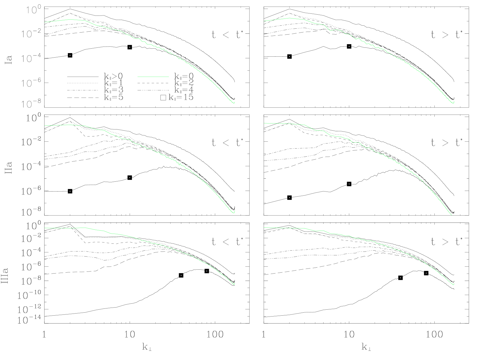
Figure 5 displays energy spectra for the Elsässer field $E^{+}(k_{\perp})$, the 3D modes $E_{w}^{+}(k_{\perp})$ and the $2$D state $E_{2D}^{+}(k_{\perp})$, at different $B_{0}$ intensity and with the same initial condition (runs Ia to IIIa). The comparison is made between two times, $t<t^{*}$ and $t>t^{*}$, where $t^{*}$ is the time from which the external force is suppressed. Shortly after the beginning of the simulations we observe that the energy spectrum $E^{+}_{2D}(k_{\perp})$ loads up. For $B_{0}=1$ this spectrum remains for all times about one order of magnitude smaller than $E_{w}^{+}(k_{\perp})$. The situation is different for stronger magnetic intensity like $B_{0}=15$. In this case, we see that $E^{+}_{2D}(k_{\perp})$ may dominate $E_{w}^{+}(k_{\perp})$ at small perpendicular wavenumbers, i.e. $k_{\perp}<10$. Then, the spectrum $E^{+}(k_{\perp})$ is formed at large scales mainly by the 2D state and at small scales by the 3D modes. Run IIa is an intermediate case where the 2D state becomes dominant in a very narrow range of perpendicular wavenumbers. The second interesting comment is about the break observed in some 3D modes spectrum just after the domain of excitation which is limited in particular to $k_{\perp}\in[1,2]$ (see relation (7)). This break appears for strong $B_{0}$ and during the driving phase. Indeed, shortly after time $t^{*}$ an extended power law energy spectrum is formed. At this resolution the driving prevents the possibility to measure any power law for the energy spectrum of the 3D modes; it is believed that it could also artificially modify the power law of the Elsässer energy spectra. Note that a similar break was already observed in driven MHD turbulence [36]. Finally, at time larger than $t^{*}$ the system evolves freely and the slope at the lowest $k_{\perp}$ is modified slightly for strong $B_{0}$ and strongly for $B_{0}=1$ with a flattening for the energy spectrum of the 3D modes: the slope goes from $k_{\perp}^{3}$ initially to roughly $k_{\perp}^{2}$ after $t^{*}$. Note that $E^{-}(k_{\perp})$, $E^{-}_{w}(k_{\perp})$ and $E^{-}_{2D}(k_{\perp})$ (not shown) exhibit a similar behavior.

Figure 6: Energy spectra $E^{+}(k_{\perp},k_{\parallel})$ at fixed $k_{\parallel}$ and for $B_{0}=1$ (top), $B_{0}=5$ (middle) and $B_{0}=15$ (bottom) which correspond to runs ${\bf Ia}$, ${\bf IIa}$ and ${\bf IIIa}$ respectively. Spectra are displayed at times $t<t^{*}$ (left) and $t>t^{*}$ (right) which are the same as in Fig. 5. The values chosen for $k_{\parallel}$ are $1,2,3,4,5,15$. For comparison we also plot the spectra of the 2D state (green color online, grey line) for which $k_{\parallel}=0$ and of the 3D modes.

The bidimensional Elsässer energy spectra $E^{+}(k_{\perp},k_{\parallel})$ are plotted in Fig. 6 at fixed $k_{\parallel}$. We choose the values $k_{\parallel}=0$ to $5$ and also $k_{\parallel}=15$. As in Fig. 5 a comparison is made between two times, $t<t^{*}$ and $t>t^{*}$. The most remarkable feature is that the spectra at fixed $k_{\parallel}$ are characterized by a pinning effect with a convergence of the spectra at large $k_{\perp}$. The case $B_{0}=15$ is an exception where the pinning is observed only for close values of $k_{\parallel}$ as we can see with a significant difference for $k_{\parallel}=15$. Note that the spectrum of the 2D state has a slightly different behavior since it does not converge towards the other spectra at large $k_{\perp}$. The second observation is that at times larger than $t^{*}$ power laws are detected for spectra with $k_{\parallel}=0$ to $5$, with a reduction of the inertial range while the power law index seems unchanged. The inertial ranges are then shifted to larger $k_{\perp}$.

Figure 7: Energy spectra $E^{\pm}(k_{\perp})$ compensated by $k_{\perp}^{2}$ (solid), $k_{\perp}^{3/2}$ (dash) and $k_{\perp}^{5/3}$ (dot) at times $t<t^{*}$ (left), $t>t^{*}$ (right), for runs ${\bf IIa}$ and ${\bf IIIa}$. Note that the times are the same as in Fig. 5.

Figure 7 presents unidimensional Elsässer energy spectra $E^{\pm}(k_{\perp})$ defined by relation (30). These spectra are compensated by different power laws $k_{\perp}^{m}$ with $m=3/2$, $5/3$ and $2$ which correspond to the predictions for strong and weak turbulence. Only runs IIa and IIIa are shown for which respectively $B_{0}/b_{rms}=2.5$ and $7.1$ (run Ia behaves similarly to run IIa). We see that run IIa fits well with power laws like $k_{\perp}^{-3/2}$ or $k_{\perp}^{-5/3}$ whereas run IIIa is close to $k_{\perp}^{-2}$. These results are in relatively good agreement with the characteristic timescales given in Table 1 which satisfy relations $\tau_{A}\sim\tau_{nl}$ for run IIa and $\tau_{A}\ll\tau_{nl}$ for run IIIa. We also see that for run IIIa the inertial range is significantly larger for $E^{+}$ than $E^{-}$. We will come back to this point below and show that the 2D state may explain such a feature.

IV.2 Runs IIIa and IIIb

Figure 8: Energy spectra $E^{\pm}(k_{\perp})$ (run ${\bf IIIb}$) for times $t=t^{*}=5.1$ (left) and $t=5.2$ (right) compensated by $k_{\perp}^{2}$ (solid), $k_{\perp}^{3/2}$ (dash) and $k_{\perp}^{5/3}$ (dot).

In this Section a comparison is made between runs IIIa and IIIb for which $B_{0}=15$. The difference between these runs comes from the initial conditions and the external force (see Table 1 and Sec. II.2).

Figure 8 shows the compensated energy spectra $E^{\pm}(k_{\perp})$ for run $\bf{IIIb}$. As in Fig. 7 spectra are compensated by different power laws $k_{\perp}^{m}$ with $m=3/2$, $5/3$ and $2$. We observe the same characteristics as for run $\bf{IIIa}$ with in particular timescales compatible with relation $\tau_{A}\ll\tau_{nl}$ (see Table 1). The only one difference is the size of the inertial ranges which are about the same for both spectra.

Figure 9: Temporal evolution of the ratios $E_{w}^{\mp}/E_{2D}^{\pm}$ for runs ${\bf IIIa}$ (top) and ${\bf IIIb}$ (bottom).

In order to explain the previous observations and the difference between cases $\bf{IIIa}$ and $\bf{IIIb}$ we shall analyze the ratios $E_{w}^{\mp}/E_{2D}^{\pm}$. We first remind that in the regime of wave turbulence the wavevectors (${\bf k}$, ${\bf p}$, ${\bf q}$) satisfy the resonant triadic interactions ${\bf k}={\bf p}+{\bf q}$ and for example $\omega({\bf k})=\omega({\bf p})-\omega({\bf q})$ which leads to the resonance condition $q_{\parallel}=0$ and to the prediction that only a spectral transfer transverse to ${\bf B_{0}}$ happens. It also means that we always have an interaction between an Alfvén wave packet of one type of polarity and the fluctuations of the 2D state with the opposite polarity. Numerical simulations have confirmed that the resonant interactions become dominant for large $B_{0}/b_{rms}$ [22]. Therefore, the amount of energy in the 2D state is an important parameter for the nonlinear dynamics. For example, the absence of energy inside the 2D state cannot lead to the development of a wave turbulence regime. In Fig. 9 the ratios $E_{w}^{\mp}/E_{2D}^{\pm}$ between the energies of the 3D modes and the 2D state with opposite polarities are given. For run ${\bf IIIb}$, we see that these ratios are almost the same and reach roughly a stationary state for times $t\in[4,6]$ with values close to $1.5$. In this regime we have $E_{2D}^{+}\sim 0.59E_{w}^{-}$ and $E_{2D}^{-}\sim 0.66E_{w}^{+}$ which lead to similar spectra $E^{\pm}(k_{\perp})$ (see Fig. 8) with inertial ranges of the same size. For run ${\bf IIIa}$ the ratios are significantly different: in the stationary phase for which $t\in[4,6]$ we have $E_{2D}^{+}\sim 0.33E_{w}^{-}$ and $E_{2D}^{-}\sim E_{w}^{+}$. In practice, the energy in the 2D state with a positive polarity is reduced which leads to a weakening of the nonlinear dynamics and a reduction of the inertial range for $E_{w}^{-}(k_{\perp})$ as we can see in Fig. 7. Note that similarly to run ${\bf IIIa}$ (see Fig 1) the energy contained in the 2D state for run ${\bf IIIb}$ represents $2/3$ of the total energy.

Figure 10: Energy spectra $E^{+}(k_{\perp},k_{\parallel})$ (top) and $E^{-}(k_{\perp},k_{\parallel})$ (bottom) at fixed $k_{\parallel}$ (run ${\bf IIIb}$) and at time $t=5.5>t^{*}$. The values chosen for $k_{\parallel}$ are $1,2,3,4$ (same notation as in Fig. 6). For comparison we also plot the spectra of the 2D state (solid) and of the 3D modes (bold solid).

Figure 10 displays spectra $E_{w}^{\pm}(k_{\perp})$, $E_{2D}^{\pm}(k_{\perp})$ and $E^{\pm}(k_{\perp},k_{\parallel})$ for $k_{\parallel}=1,2,3,4$. Globally we observe the same features as for run ${\bf IIIa}$ with a stronger domination of the 2D state at large scales. Note that at the smallest $k_{\perp}$, the initial power law in $k_{\perp}^{2}$ applied to spectra $k_{\parallel}=1,2$ is slightly modified and the scaling for $E_{w}^{\pm}(k_{\perp})$ is unchanged. Note also that the break previously reported for times $t<t^{*}$ is also observed (not shown). Finally, as we have already seen in Fig 5 (run $\bf{IIIa}$), for times $t>t^{*}$ an inertial range appears for spectra $E_{w}^{\pm}(k_{\perp})$ and $E^{\pm}(k_{\perp},k_{\parallel})$ with $k_{\parallel}=1,2,3,4$ which seem roughly better fitted by $k_{\perp}^{-3/2}$ or $k_{\perp}^{-5/3}$ than $k_{\perp}^{-2}$.

Figure 11: Temporal evolution of Alfvén ratios $r^{A}(t)$ (solid), $r^{A}_{2D}(t)$ (dash) and $r^{A}_{w}(t)$ (dot) for run ${\bf IIIb}$.

Figure 11 shows eventually the time variations of the Alfvén ratios $r^{A}(t)$, $r^{A}_{2D}(t)$ and $r^{A}_{w}(t)$. The main difference between run ${\bf IIIa}$ (see Fig. 3) and run ${\bf IIIb}$ resides first in the initial values which are larger for the latter run. The evolution is also different with a variation of all quantities during the driving phase. It is only during the decay phase that we recover the same behavior as in run ${\bf IIIa}$ with alfvénic fluctuations and an equipartition for the 3D modes. In this decay phase, a large deviation of $r^{A}_{w}(t)$ is observed immediately after $t^{*}$ in order to reach the equipartition which clearly means that it is the natural state of the system (in ${\bf IIIa}$ the situation was not totally clear since before $t^{*}$ we were already at equipartition).

V Summary and conclusion

In this paper, we present a set of 3D direct numerical simulations of incompressible driven MHD turbulence under the influence of a uniform magnetic field ${\bf B_{0}}$. In particular, the temporal and spectral properties of the 2D state (or slow mode) are investigated. We show that if initially the energy contained in the 2D state is set to zero it becomes shortly non negligible in particular when the intensity of $B_{0}$ is strong. For our larger $B_{0}$ intensity ($B_{0}=15$) this energy saturates in the stationary phase around $2/3$ of the total energy whereas the energy of the 3D modes remains roughly constant. We also observed that the ratio $B_{0}/b_{rms}$ saturates around $7$ for both simulations with $B_{0}=15$ with initially a ratio equal to $15$ (run ${\bf IIIa}$) and to $19$ (run ${\bf IIIb}$). In all situations, the magnetic energy dominates the kinetic energy but it is shown that at large $B_{0}/b_{rms}$ and in the decay phase the natural state for the 3D modes is the equipartition whereas the 2D state is magnetically dominated. It is interesting to note that a theoretical model in terms of condensate has been recently proposed to explain the spontaneous generation of a residual energy $E^{v}-E^{b}$ at small $k_{\parallel}$ [27]. This model is based on the breakdown of the mirror-symmetry in unbalanced wave turbulence.

From a spectral point of view, when the $B_{0}$ intensity is strong enough the $k_{\perp}$–energy spectra are mainly composed at large scales by the 2D state and at small scales by the 3D modes. This situation is similar to rotating turbulence for neutral fluids [37, 38] where in particular the nonlinear transfers are reduced along the rotating rate [39]. However, a detailed analysis of the temporal evolution of the 2D state energy spectra shows that a direct cascade happens whereas for rotating turbulence an inverse cascade is generally evoked [40]. The same remark holds for energy spectra at fixed $k_{\parallel}>0$ where we observe additionally a pinning effect at large $k_{\perp}$. According to the value of $B_{0}/b_{rms}$ scalings close to $k_{\perp}^{-3/2}$ – $k_{\perp}^{-5/3}$ or $k_{\perp}^{-2}$ are found which are in agreement with different predictions for strong and wave turbulence [8, 9, 14, 19].

The external force seems to be an important parameter for the dynamics. For example in [25] a change of spectral slope was reported for the $k_{\perp}$–energy spectrum when the intensity of $B_{0}$ is modified. In this work the external force was applied at $k_{\parallel}>0$ and $k_{\perp}=1,2$. In [18] a forcing which kept the ratio of fluctuations to mean field approximately constant was implemented by freezing modes $k\leq 2$ and a spectral slope close $k_{\perp}^{-3/2}$ was reported for $B_{0}=5$. The fact that the 2D state was imposed by the forcing has certainly an impact on the nonlinear dynamics since it prevents the natural growth of the 2D state energy at small $k_{\perp}$. We remind that the 2D state is essential at large $B_{0}/b_{rms}$ since it mainly drives the nonlinear dynamics. In particular, we observe that a reduction of the 2D state energy of one type of polarity leads to a decrease of the inertial range of the 3D modes energy spectrum with the opposite polarity.