Increasing the Fisher information content in the matter power spectrum by non-linear wavelet Wiener filtering

Abstract

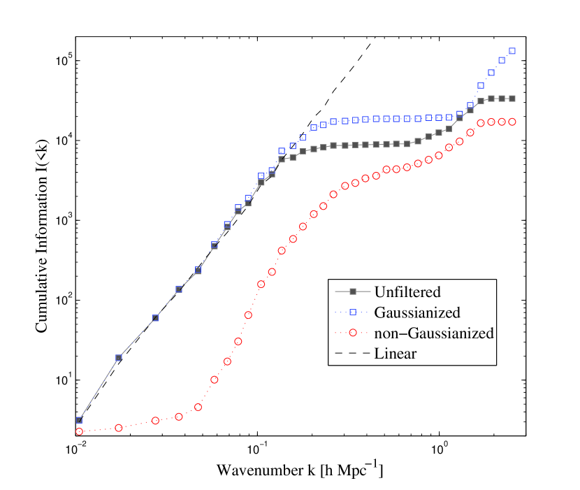
We develop a purely mathematical tool to recover some of the information lost in the non-linear collapse of large-scale structure. From a set of 141 simulations of dark matter density fields, we construct a non-linear Wiener filter in order to separate Gaussian and non-Gaussian structure in wavelet space. We find that the non-Gaussian power is dominant at smaller scales, as expected from the theory of structure formation, while the Gaussian counterpart is damped by an order of magnitude on small scales. We find that it is possible to increase the Fisher information by a factor of three before reaching the translinear plateau, an effect comparable to other techniques like the linear reconstruction of the density field.

1. Introduction

In modern cosmology, the power spectrum of matter fluctuations, $P(k)$, is a key measurement, as it is related to many cosmological parameters. Recent observations such as the cosmic microwave background (Komatsu et al., 2009), the correlation function of galaxies (Eisenstein et al., 2005; Tegmark et al., 2006; Percival et al., 2007b, a, 2010), the strong gravitational lensing probability for image separation (Chen, 2003; Chen & Zhao, 2006; Oguri, 2006), and the shear correlation function for weak gravitational lensing (Pen et al., 2003; Hoekstra et al., 2006; Benjamin et al., 2007; Fu et al., 2008), have been able to but constraints on many parameters. In many analyses, cosmologists are interested in measuring the matter power spectrum on large scales, which holds a wealth of cosmological information that has not been erased by the non-linear gravitational collapse. The constraining strength of a survey depends directly on the amount of Fisher information (Fisher, 1935; Tegmark et al., 1997), i.e. statistically independent Fourier modes, contained in the measurement, and one needs to maximize the information in order to minimize the uncertainty on cosmological parameters.

Rimes & Hamilton (2005, 2006) first studied the amount of Fisher information as a function of scale contained in the matter power spectrum. They estimated the information content about the initial amplitude of the linear power spectrum from an ensemble of many $N$-body simulations and showed that the Fisher information is preserved in the matter power spectrum on large, linear scales. They also observed that the information plateaus in the translinear regime ($k\sim 0.2-0.8h/{\rm Mpc}$), and that there is a second increase in information when including the small, non-linear scales. Neyrinck et al. (2006) then found that the halo model also predicts this behavior on translinear scales in the information content, which comes largely from cosmic variance in the number of the largest haloes in a given volume. Furthermore, Neyrinck & Szapudi (2007) found that the cosmological Fisher information in the matter power spectrum about many key cosmological parameters is quite degenerate both on translinear and non-linear scales. They also showed that it can be difficult to constrain the initial cosmological conditions from the dark matter power spectrum on non-linear scales, and suggested the removal of the largest haloes as an alternative to resolve this problem. Based on the technique of Rimes & Hamilton (2005, 2006), Lee & Pen (2008) estimate the Fisher information in the galaxy angular power spectrum from the photometric redshift catalogue of the Sloan Digital Sky Survey Data Release 5. Their results also show that very little new information is contained in the matter density power spectrum on the translinear scale, which is observationally consistent with the previous numerical trend (Rimes & Hamilton, 2005, 2006; Hamilton et al., 2006; Neyrinck et al., 2006; Neyrinck & Szapudi, 2007).

Many methods have been proposed to recover parts of this lost information, notably running $N$-body simulations backwards in time (Goldberg & Spergel, 2000), or density field reconstruction from linear theory (Eisenstein et al., 2007; Noh et al., 2009; Padmanabhan et al., 2009). Neyrinck et al. (2009) introduces a method of logarithmic mapping of the density field, successfully recover great amount of information content in the dark matter power spectrum. Weinberg (1992) uses a method called Gaussianization, which is a monotonic transformation of the smoothed galaxy distribution to reconstruct primordial density fluctuations. Here we attempt to Gaussianize the density fields by non-linear Wiener filtering. Our objective is to filter out the non-linear structure, leaving behind a density field in which the amount of Fisher information has increased.

Structure formation in current theories starts from an initially linear Gaussian random field, which progressively becomes non-linear through gravitational instabilities, starting at the smallest scales. This process is local in real space, and only the linear part of the field remains intrinsically Gaussian. In the non-linear regime, the Fourier modes start to couple together, and the field is no longer Gaussian. It is legitimate to ask how to filter out the non-linearities. Wavelet functions provide a natural basis that compromises between the locality in real and Fourier space. Moreover, it can simultaneously decompose the data, functions or even operators in coordinate (or time) space and scale (or frequency) space. Therefore, wavelet transforms are an ideal numerical technique for extracting multi-scale information (Fang & Thews, 1998), as required by our Wiener filter. Pando & Fang (1996) applied this method to the high redshift L$\alpha$ systems, which often have separations on translinear scales. Pen (1999) also discussed the application of wavelets to filter the Gaussian noise contained in some images, and found that the wavelet basis is highly advantageous over the standard Fourier basis if the data are intermittent in nature.

In this paper, we apply the wavelet method in order to push the translinear plateau further in the information content, without removing the largest haloes in the analysis. The outline of the paper is as follows. In §2, we present the $N$-body code that was used to simulate the dark matter density fields. In §3, we discuss the application of the discrete wavelet transform (DWT) and Bayesian theory to filter out some of the non-Gaussian component of the density fields. In §4, we compare the power spectra of the filtered and unfiltered data, while in §5 we analyze the information content in both data sets. Discussion and conclusions are presented in §6.

2. $N$-body Simulations of dark matter density fields

We use the cosmological simulation code CubeP3M (CITA Computing 2008), an upgraded version of PMFAST (Merz et al., 2005) that uses a cubical decomposition instead of slabs in the global FFT, and thus scales to much larger runs. In addition, the gravitational force is now calculated down to the subgrid level, which increases the code resolution. Finally, it is both MPI and openmp parallelized, perfect for running on most computer clusters.

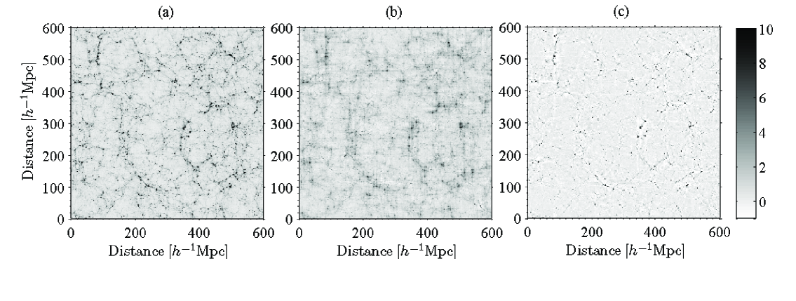
We run 141 simulations with a box size of 600 $h^{-1}$ Mpc and a resolution of $512^{3}$ cells and $256^{3}$ particles. The initialization step of the simulation first reads a CMBFAST (Seljak & Zaldarriaga, 1996) transfer function, which models our fiducial cosmology, and evolves the power linearly to an initial redshift of $z=200$. It then uses the Zel’dovich approximation to calculate a displacement field and a velocity field, which are assigned to the initial particles. The cosmological parameters used are $\Omega_{\rm M}=0.29$, $\Omega_{\Lambda}=0.71$, $h=0.73$, $\sigma_{8}=0.84$, and $n_{s}=0.95$. The code then evolves these initial densities up to $z=0$. One of those density fields is plotted in Fig.3(a). For the purpose of visualization, the 3D field is projected onto a 2D plane by averaging over part of the third dimension.

3. Non-Gaussian filtering of density fields

3.1. Discrete wavelet transform (DWT)

Similar to the Fast Fourier Transform (FFT), the Discrete Wavelet Transform (DWT) is an invertible, linear operation, and can be considered as a rotation in function space. Both operations transform a data vector, whose length must be an integer power of 2, to a numerically different vector of the same length. The FFT’s basis functions are sines and cosines, which, of course, are not localized in real space. The DWT, on the other hand, has two kinds of basis functions, called scaling functions (mother functions) and difference functions (wavelet functions). Unlike sines and cosines, individual DWT basis functions are localized both in real and frequency space, and because they vary both in scales and locations, they enable us to analyze more accurately the fine variations in a data set.

Although there is an infinite number of possible forms of DWT basis functions, only a few have a clear meaning. The simplest discrete wavelet is the Haar wavelet, which suffers from the fact that its basis functions are discontinuous and provide a poor approximation to smooth functions. We consider in this paper the Daubechies-4 wavelet basis (hereafter DB-4) (Daubechies, 1992), which contains families of scaling functions and wavelets that are orthogonal, continuous and have compact support.

We denote the one-dimensional scaling function and wavelet function as $\phi$ and $\psi$. For simplicity we first consider a one-dimensional vector $\mathbf{d}(\vec{x})$ with length $L=2^{J}$. Using DB-4 wavelet, it can be expanded as

$$d(x)=\sum_{l=0}^{1}\epsilon_{0,l}\phi_{0,l}(x)+\sum_{j=0}^{J-1}\sum_{l=0}^{2^{j}-1}\tilde{\epsilon}_{j,l}\psi_{j,l}(x),$$ (1)

where $j$ and $l$ can be regarded as a dilation and a translation of the basis function:

$$\phi_{j,l}(x)=\sqrt{\frac{2^{j}}{L}}\phi(2^{j}x/L-l)$$ (2)

$$\psi_{j,l}(x)=\sqrt{\frac{2^{j}}{L}}\psi(2^{j}x/L-l).$$ (3)

$\epsilon_{j,l}$ and $\tilde{\epsilon}_{j,l}$ are called scaling function coefficients (hereafter SFCs) and wavelet function coefficients (hereafter WFCs). They can be calculated by

$$\epsilon_{j,l}=\int d(x)\phi_{j,l}(x){\rm d}x,$$ (4)

and

$$\tilde{\epsilon}_{j,l}=\int d(x)\psi_{j,l}(x){\rm d}x.$$ (5)

Any particular set of wavelets is specified by a corresponding set of wavelet filter coefficients. The most localized Daubechies wavelet is DB-4 wavelet. Its scaling and wavelet functions have 4 coefficients, $a_{0},...,a_{3}$ and $b_{-1},...,b_{1}$ respectively.

$$a_{0}=(1+\sqrt{3})/4,\ \ \ \ a_{1}=(3+\sqrt{3})/4,$$

$$a_{2}=(3-\sqrt{3})/4,\ \ \ \ a_{3}=(1-\sqrt{3})/4,$$

and

$$b_{-2}=(1-\sqrt{3})/4,\ \ \ \ b_{-1}=(\sqrt{3}-3)/4,$$

$$b_{0}=(3+\sqrt{3})/4,\ \ \ \ b_{1}=(\sqrt{3}-1)/4.$$

The wavelet transform of a vector of data is done first by applying a wavelet coefficient matrix to the whole vector, and then applying a “smaller” matrix to the smoothed vector of length $L/2$. For DB-4 wavelet transform, this was done until only two SFCs were left. Finally, two SFCs store the information of the mean of the largest scale of the vector, and $L-2$ WFCs store the information of the fluctuations or the differences between regions of the vector. For 3D simulation data, the process is similar. The data is wavelet transformed in one arbitrary direction $x_{1}$, the result is transformed in another direction $x_{2}$, and then in $x_{3}$. Finally, the result contains $2^{3}=8$ SFCs and $512^{3}-8$ WFCs.

3.2. Non-linear filtering

We now have the DWT transform of those density fields which we need to filter. Because of the linearity of wavelet transforms, we can think of the data as being filtered into two pieces, the inverse wavelet transforms of which are called the Gaussianized density $\mathbf{d}_{a}$ and the non-Gaussianized density $\mathbf{d}_{b}$. The unfiltered density fields $\mathbf{d}$ consist of the sum of these two parts, and the hope is that the Gaussianized density will be closer to linear theory. Since the filtering process is in wavelet space, we divided the wavelet transform of the density field $\mathbf{D}$ into the Gaussianized part $\mathbf{A}$ and the non-Gaussianized part $\mathbf{B}$. Again, because of the linearity of wavelet transforms, we have

$$\mathbf{d}=\mathbf{d_{a}}+\mathbf{d_{b}}$$ (6)

in real-space and

$$\mathbf{D}=\mathbf{A}+\mathbf{B}.$$ (7)

in wavelet space.

The method of thresholding and Gaussian Wiener filtering is not suitable in this work, because we need to filter localized structure, so we use a non-Gaussian Wiener filter instead. In wavelet basis the non-Gaussianity is clearly represented (Pen, 1999), so the filter is applied on each wavelet modes. Each wavelet mode has three $j$ ’s to characterize the mode’s scale, and we denote wavelet modes with $\mathbf{s}$. We regard $\mathbf{A}$ as Gaussian white noise $\mathbf{N}$, as in Pen (1999), $\mathbf{B}$ as the original image $\mathbf{U}$, and $\mathbf{D}$ as the noisy image $\mathbf{D}=\mathbf{A}+\mathbf{B}$. For each wavelet mode, we assume that the WFCs $A(\mathbf{r},\mathbf{s})$, at fixed sclae $\mathbf{s}$, has the form of a Gaussian distribution $\mathcal{N}(0,\sigma^{2})$ over position $\mathbf{r}$, and if we know the PDF of $D(\mathbf{r},\mathbf{s})$, all the modes are statistically independent. We denote the PDF for a given mode of $B(\mathbf{r},\mathbf{s})$ as $\Theta(b)$, and we obtain the variable $D(\mathbf{r},\mathbf{s})$ with PDF

$$f(d)=\frac{1}{\sqrt{2\pi}}\int\Theta(b)\exp(-\frac{1}{2}(d-b)^{2}){\rm d}b$$ (8)

According to Bayes’s theorem, we can calculate the conditional probability $P(B|D)=P(D|B)P(B)/P(D)$. For the posterior conditional expectation value, we get

$$\langle B|D=d\rangle=\frac{1}{\sqrt{2\pi}f(d)}\int{\exp[-\frac{1}{2}(u-d)^{2}]\Theta(u)u{\rm d}u}$$ (9)

$$B=D+\frac{1}{\sqrt{2\pi}f(d)}\partial_{d}\int{\exp[-\frac{1}{2}(u-d)^{2}]\Theta(u){\rm d}u}$$ (10)

$$B=D+(\ln f)^{\prime}(d).$$ (11)

We define two filter functions

$$\alpha(\mathbf{s})=A/D,$$ (12)

$$\beta(\mathbf{s})=B/D,$$ (13)

so

$$\alpha(\mathbf{s})=-\frac{(\ln f)^{\prime}(d)}{d},$$ (14)

$$\beta(\mathbf{s})=1+\frac{(\ln f)^{\prime}(d)}{d}.$$ (15)

In order to realize the filtering of the actual data, we have to estimate the prior distribution $\Theta$ for each wavelet mode.

We assume that the one-point distribution of modes is non-Gaussian and that the modes are statistically independent, and so we need to specify the PDF for each mode. In this work we use Cartesian product wavelets (Meyer, 1995). This basis for our density fields has three scales $2^{J-j_{1}}$, $2^{J-j_{2}}$ and $2^{J-j_{3}}$ (in unit of pixels), which are the length, width and height of the cuboid each wavelet support in real-space. We define the volume of the cuboid in real-space as the equivalent volume $V_{e}$. For the real data, the structures dealt with have different physical scales and specific locations in the 3D density field. Consequently, the optimal basis must also depend both on the scale and the location. As mentioned before, our wavelet basis, which is localized both in frequency space and in real-space, are perfectly well suited to effectively extracting the information of these structures. Every WFC can be seen as the dot product of the density field and a wavelet of a particular scale and shape.

Since the modes are statistically independent, it is natural to collect together all the WFCs with the same corresponding cuboids, and then to obtain the PDF of this scale. Actually, we do not differentiate the direction of the cuboids and consider only the combination of $j_{1}$, $j_{2}$ and $j_{3}$. That is to say, we regard $(j_{1},j_{2},j_{3})=(1,2,3)$ and $(j_{1},j_{2},j_{3})=(1,3,2)$ as the same cuboids, and the corresponding WFCs are collected together. Note that there may be more than one combination whose equivalent volumes are the same.

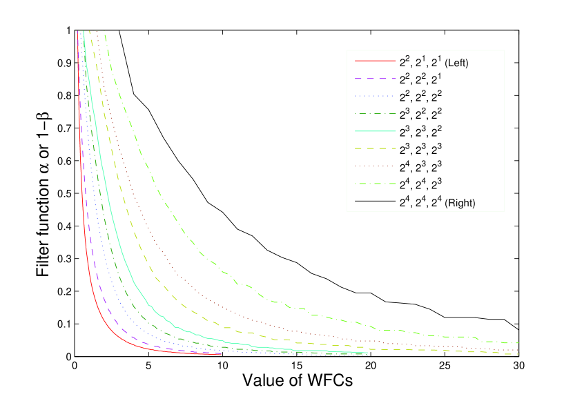
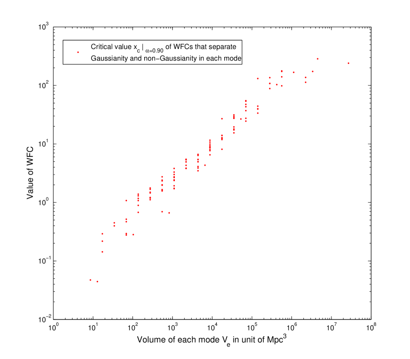
However, fewer WFCs are available for larger scales, or greater equivalent volumes, and thus the PDF has lower statistics, which makes the calculation of filter functions less accurate. If there are not enough WFCs, or if improper statistics are used, the appearance of fluctuation in the PDF, especially the region near zero where the property of Gaussianity is detected, reduces our precision in the determination of the filter functions. However, since we collect the WFCs over 141 density fields we have enough statistics to make both the PDF and filter functions smooth. Also, in counting the WFCs, we choose an adequate set of intervals, or bins, in order to best represent the shape of the PDF. The range of the intervals must both be large enough to contain the non-Gaussian ‘tails’ in the PDF, and small enough to show the detailed properties of Gaussianity. We discuss these in the next paragraph. We find that the WFCs on different scales have different distributions. The curves of PDFs where WFC’s value are relatively small appear to be Gaussian, but there are non-Gaussian ‘tails’ for larger values of PDFs. It seems that if those WFCs belong to larger scales, or larger $V_{e}$, the ‘boundary’ value between Gaussianity and non-Gaussianity is larger. We plot 9 filter functions in Fig.1 to compare the shape of the filter function curve between scales. This property is more easily visualized if we define a critical value on each scale, defined as the critical value of WFC $x_{c}$ that yields $\alpha=0.9$. In Fig.2 we plot that critical value $x_{c}$ versus $V_{e}$.

Figure 1.— Filter functions $\alpha$ and $\beta$ as a function of the WFC’s value, 9 wavelet modes are chosen. Each mode is described by a combination of three lengths, as seen in the legend, which form the cuboid that the DWT basis function governs. Moving from left to right in the plot corresponds to moving from top to bottom in the legend. As WFCs are small, one can see that $\alpha$ is simply unity, where Gaussianity dominates.

Figure 2.— Critical value of WFC $x_{c}$ of the scales versus the equivalent volume $V_{e}$ of the basis function. The $x_{c}$ is defined via $\alpha(x_{c})=0.9$, which can be regard as a boundary between Gaussianity and non-Gaussianity on that scale.

The CDF of a set of data is obtained by sorting and by doing derivatives to get the PDF. However, it is challenging to sort all the WFCs on one scale among hundreds of density fields. Instead, we first construct several hundreds of interval bins, and then read every density field datum to check the WFCs on each scale, and find which interval each of these WFCs belongs to. Actually, there are a total 120 different scales, so we need to count all the WFCs on each scale and on each of the 141 densities to produce our final 120 PDFs of WFCs. Then, we check each of these PDFs, and determine whether the intervals properly represent the shape of PDFs. If not, we may try another series of bins, get a new set of PDFs, and iterate until all the PDFs have been measured.

We also use i) the same set of simulations but with lower resolution, and ii) new set of simulations with finer resolution, and get similar PDFs of WFCs (thus filter functions) on same physical scales. As a result, the resolution of simulations does not affect WFCs’ PDF if the physical scales are the same.

From the relationship between the critical values and $V_{e}$, we can see that for smaller scales, the critical values are smaller, such that the signal contributes more to the non-Gaussian density field, as expected.

We finally filter all the data by multiplying the densities in wavelet space with our filter functions, Eq.14 and Eq.15, which separates those 141 density fields into Gaussian and non-Gaussian contributions. Note that we do not filter the SFCs because they only govern the mean of the largest scales and have no significant impact on the power spectra. We plot a slice of an unfiltered density and its Gaussianized and non-Gaussianized components in Fig.3.

Figure 3.— (a) Map of a density field with a width of 600 $h^{-1}$ Mpc and $512^{3}$ pixels, randomly selected from 141 $N$-body simulations. A slice of the density field is projected onto the x-y plane for visualization. (b) Same as (a), but the map is Gaussianized by wavelet filtering. (c) Same as (a), but the map is non-Gaussianized by wavelet filtering. (b) and (c) add up to (a).

4. Comparison of power spectra

The power spectrum is the Fourier transform of the correlation function and measures the amount of clustering in the matter distribution. It is measured in terms of the wavenumber $k$ in units of $h{\rm Mpc}^{-1}$. In the case of a Gaussian random field, the power spectrum describes completely the statistics of the distribution, as all high moments either vanish or factor into its explicit functions. The power spectrum from each simulation is defined as

$$\langle|\delta(\vec{k},\vec{k^{\prime}})|\rangle^{2}=(2\pi)^{3}P(\vec{k})\delta(\vec{k}-\vec{k^{\prime}}),$$ (16)

where $\langle|\delta(\vec{k},\vec{k^{\prime}})|\rangle^{2}$ is the volume average of the expectation value and $P(\vec{k})$ is the power spectrum. Of equal interest is $\Delta^{2}_{k}$, the power spectrum in its dimensionless form, defined as:

$$\Delta^{2}_{k}\equiv\frac{k^{3}P(k)}{2\pi^{2}}.$$ (17)

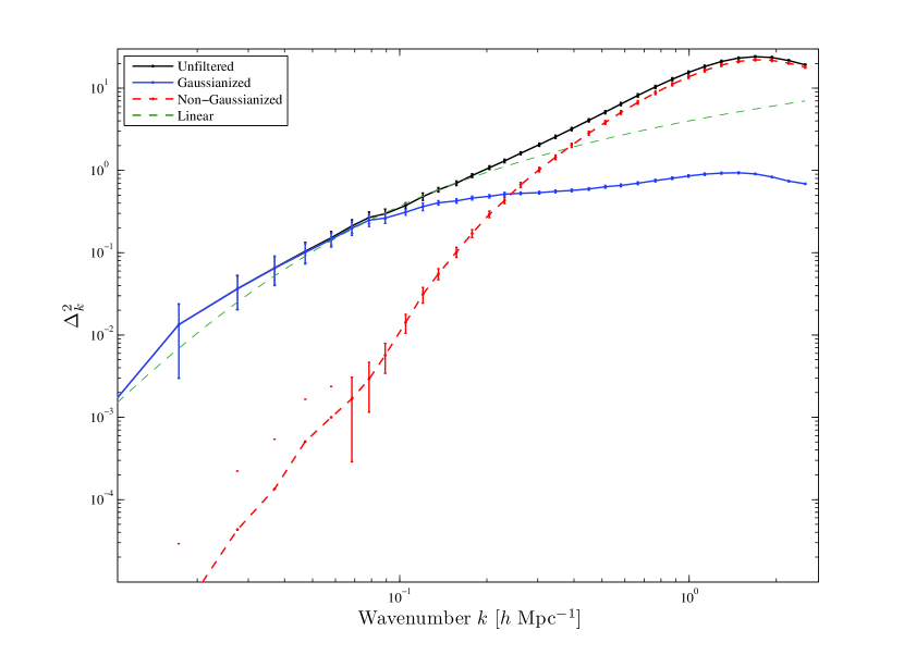
For the 141 simulations, Gaussianized and non-Gaussianized densities are generated, as described in the previous section. The power spectra of these 423 mass distributions are calculated using the ‘Nearest Grid Point’ (NGP) mass assignment scheme, which calculates the position of each particle based on which grid point it is nearest. In Fig.4 we plot the mean power spectrum and error bars of 141 unfiltered, Gaussianized and non-Gaussianized density fields. We can see that for small $k$, corresponding to large scales, Gaussianized fluctuations dominate the power, and that for large $k$, corresponding to small scales, non-Gaussianized fluctuations dominate. Non-Gaussianized fluctuations begin to dominate the power in the region $k\sim 0.2$, which is the boundary of the linear power spectrum and the non-linear power spectrum. We can see that the non-Gaussian filter in wavelet space is quite efficient at separating the linear and non-linear power spectra.

Figure 4.— Power spectra and error bars of the density field simulations, and their Gaussianized and non-Gaussianized power spectra. Each curve is determined by the mean of over 141 power spectrum samples, and the error bars describe those standard deviations. The error was multiplied by 3. The BBKS linear power spectrum is plotted in dash line.

5. Information content in the power spectra of density fields

The covariance is the mean value of the product of the deviations of two variables from their respective means. Simply put, it measures the correlation between the variance, or the error bars, of the power spectra at different scales $k$. If the measurements were completely uncorrelated, the diagonal of the covariance matrix would be the variance at each value of k, and all the off-diagonal entries would be zero. Mathematically, the covariance matrix is defined as

$$C(k,k^{\prime})\equiv\frac{1}{N-1}\sum_{i=1}^{N}[P_{i}(k)-\langle P(k)\rangle][P_{i}(k^{\prime})-\langle P(k^{\prime})\rangle],$$ (18)

where $N$ is the number of realizations and $\langle P(k)\rangle$ is the mean power spectrum.

The cross-correlation coefficient matrix, or for short the correlation matrix, is a normalized version of the covariance matrix, where each value is divided by the square root of the diagonal values as follows:

$$\rho(k,k^{\prime})=\frac{C(k,k^{\prime})}{\sqrt{C(k,k)C(k^{\prime},k^{\prime})}}.$$ (19)

The three correlation matrices for our unfiltered, Gaussianized and non-Gaussianized densities are shown in Fig.5. For the covariance matrix of the unfiltered densities, the linear regime is diagonal, while in the non-linear regime, the power spectra at different $k$-modes are correlated by at least 40%. In the Gaussian filtered covariance matrix, however, we find a smaller correlated region. It seems that the correlations between $k$-modes are suppressed to some extent. When we look at the non-Gaussian filter, we see that the diagonal is now a few cells thick, i.e. some non-diagonal elements are correlated even in the linear regime. This is allowed, since the ‘Gaussian + non-Gaussian’ decomposition is done on the densities, not on the covariance matrix. Also, the corresponding value in the covariance matrix are many orders of magnitude smaller than those in the unfiltered and Gaussian cases, and thus play no role what so-ever.

Figure 5.— (a) Cross-correlation coefficient matrix as found from 141 power spectra of the density field simulations. The squares in black on the diagonal line indicate perfect correlation. (b) Same as (a), but the power spectra are from the Gaussianized density fields. (c) Same as (a), but the power spectra are from the non-Gaussianized density fields.

The cumulative Fisher information is defined as follows: for a given wavenumber, we select a subsection of the covariance matrix to that wavenumber, and we invert this sub-matrix, and sum over all its elements. The normalized covariance matrix is described as follows

$$C_{\rm norm}(k,k^{\prime})=\frac{C(k,k^{\prime})}{\langle P(k)\rangle\langle P(k^{\prime})\rangle},$$ (20)

and our cumulative information function is

$$I(k_{n})=\sum_{i,j=1}^{n}C_{\rm norm}^{-1}(k_{i},k_{j}).$$ (21)

We plot the cumulative information of the unfiltered, Gaussianized and non-Gaussianized power spectra in Fig.6. One can see that in the translinear regime, where $k\sim 0.2$, the cumulative information of the density fields has a flat plateau, which indicates that there is nearly no independent information in the non-linear regime of the power spectrum. In comparison, for the Gaussianized information, the cumulative information also has a plateau, but at a higher value, which indicates that it contains about three times more independent Fourier modes. This is a key result, especially for parameter estimation obtained through Fisher matrices. These analyses could be improved by up to a factor of $\sqrt{3}$ solely by filtering their data.

Figure 6.— Cumulative information in the power spectra as a function of the wavenumber. The black squares filled with grey correspond to the density field simulations without filtering. The blue squares and the blue solid line correspond to the Gaussianized densities. The red squares and the red dashed line correspond to the non-Gaussianized densities.

6. Conclusion

We use the code ‘CubeP3M’ to generate 141 dark matter density fields. In wavelet space, we construct a non-Gaussian Wiener filter in order to separate non-Gaussian and Gaussian structures. We measure the power spectra of the unfiltered, Gaussianized and non-Gaussianized density fields, and find that the Gaussianized power spectrum is heavily dampened on small scales, while the non-Gaussian features dominate at smaller scales, as expected from structure formation. We also calculate the cumulative information, and find that the plateau in the translinear regime rises in the Gaussianized information curve by a factor of three.

References

- Benjamin et al. (2007) Benjamin, J. et al. 2007, MNRAS, 381, 702, arXiv:astro-ph/0703570
- Chen (2003) Chen, D. 2003, ApJ, 587, L55, arXiv:astro-ph/0301037
- Chen & Zhao (2006) Chen, D., & Zhao, H. 2006, ApJ, 650, L9, arXiv:astro-ph/0606506
- Daubechies (1992) Daubechies, I. 1992, Ten Lectures on Wavelets (C B M S - N S F Regional Conference Series in Applied Mathematics) (Soc for Industrial & Applied Math)
- Eisenstein et al. (2005) Eisenstein, D. J., Blanton, M., Zehavi, I., Bahcall, N., Brinkmann, J., Loveday, J., Meiksin, A., & Schneider, D. 2005, ApJ, 619, 178, arXiv:astro-ph/0411559
- Eisenstein et al. (2007) Eisenstein, D. J., Seo, H., Sirko, E., & Spergel, D. N. 2007, ApJ, 664, 675, arXiv:astro-ph/0604362
- Fang & Thews (1998) Fang, L.-Z. e., & Thews, R. L. e. 1998, Wavelets in Physics (Singapur: World Scientific)
- Fisher (1935) Fisher, R. A. 1935, Journal of the Royal Statistical Society, 98, 39
- Fu et al. (2008) Fu, L. et al. 2008, A&A, 479, 9, 0712.0884
- Goldberg & Spergel (2000) Goldberg, D. M., & Spergel, D. N. 2000, in Astronomical Society of the Pacific Conference Series, Vol. 201, Cosmic Flows Workshop, ed. S. Courteau & J. Willick, 282–+, arXiv:astro-ph/9909057
- Hamilton et al. (2006) Hamilton, A. J. S., Rimes, C. D., & Scoccimarro, R. 2006, MNRAS, 371, 1188, arXiv:astro-ph/0511416
- Hoekstra et al. (2006) Hoekstra, H. et al. 2006, The Astrophysical Journal, 647, 116
- Komatsu et al. (2009) Komatsu, E. et al. 2009, ApJS, 180, 330, 0803.0547
- Lee & Pen (2008) Lee, J., & Pen, U.-L. 2008, ApJ, 686, L1, 0807.1538
- Merz et al. (2005) Merz, H., Pen, U.-L., & Trac, H. 2005, New Astronomy, 10, 393, arXiv:astro-ph/0402443
- Meyer (1995) Meyer, Y. 1995, Wavelets and Operators: Vol. 37 (Cambridge Studies in Advanced Mathematics) (Cambridge University Press)
- Neyrinck & Szapudi (2007) Neyrinck, M. C., & Szapudi, I. 2007, MNRAS, 375, L51, arXiv:astro-ph/0610211
- Neyrinck et al. (2006) Neyrinck, M. C., Szapudi, I., & Rimes, C. D. 2006, MNRAS, 370, L66, arXiv:astro-ph/0604282
- Neyrinck et al. (2009) Neyrinck, M. C., Szapudi, I., & Szalay, A. S. 2009, ApJ, 698, L90, 0903.4693
- Noh et al. (2009) Noh, Y., White, M., & Padmanabhan, N. 2009, Phys. Rev. D, 80, 123501, 0909.1802
- Oguri (2006) Oguri, M. 2006, MNRAS, 367, 1241, arXiv:astro-ph/0508528
- Padmanabhan et al. (2009) Padmanabhan, N., White, M., & Cohn, J. D. 2009, Phys. Rev. D, 79, 063523, 0812.2905
- Pando & Fang (1996) Pando, J., & Fang, L. 1996, ApJ, 459, 1, arXiv:astro-ph/9504037
- Pen et al. (2003) Pen, U., Lu, T., van Waerbeke, L., & Mellier, Y. 2003, MNRAS, 346, 994, arXiv:astro-ph/0304512
- Pen (1999) Pen, U.-L. 1999, Royal Society of London Philosophical Transactions Series A, 357, 2561, arXiv:astro-ph/9904170
- Percival et al. (2007a) Percival, W. J., Cole, S., Eisenstein, D. J., Nichol, R. C., Peacock, J. A., Pope, A. C., & Szalay, A. S. 2007a, MNRAS, 381, 1053, 0705.3323
- Percival et al. (2007b) Percival, W. J. et al. 2007b, ApJ, 657, 51, arXiv:astro-ph/0608635
- Percival et al. (2010) ——. 2010, MNRAS, 401, 2148, 0907.1660
- Rimes & Hamilton (2005) Rimes, C. D., & Hamilton, A. J. S. 2005, MNRAS, 360, L82, arXiv:astro-ph/0502081
- Rimes & Hamilton (2006) ——. 2006, MNRAS, 371, 1205, arXiv:astro-ph/0511418
- Seljak & Zaldarriaga (1996) Seljak, U., & Zaldarriaga, M. 1996, ApJ, 469, 437+
- Tegmark et al. (2006) Tegmark, M. et al. 2006, Phys. Rev. D, 74, 123507, arXiv:astro-ph/0608632
- Tegmark et al. (1997) Tegmark, M., Taylor, A. N., & Heavens, A. F. 1997, ApJ, 480, 22, arXiv:astro-ph/9603021
- Weinberg (1992) Weinberg, D. H. 1992, MNRAS, 254, 315