The architecture of Abell 1386 and its relationship to the Sloan Great Wall

Abstract

We present new radial velocities from AAOmega on the Anglo-Australian Telescope for 307 galaxies ($b_{J}<19.5$) in the region of the rich cluster Abell 1386. Consistent with other studies of galaxy clusters that constitute sub-units of superstructures, we find that the velocity distribution of A1386 is very broad (21,000–42,000 km s^-1, or $z=0.08$–0.14) and complex. The mean redshift of the cluster that Abell designated as number 1386 is found to be $\sim 0.104$. However, we find that it consists of various superpositions of line-of-sight components. We investigate the reality of each component by testing for substructure and searching for giant elliptical galaxies in each and show that A1386 is made up of at least four significant clusters or groups along the line of sight whose global parameters we detail. Peculiar velocities of brightest galaxies for each of the groups are computed and found to be different from previous works, largely due to the complexity of the sky area and the depth of analysis performed in the present work. We also analyse A1386 in the context of its parent superclusters: Leo A, and especially the Sloan Great Wall. Although the new clusters may be moving toward mass concentrations in the Sloan Great Wall or beyond, many are most likely not yet physically bound to it.

1 Introduction

Galaxies are typically found clustered together with other galaxies – whether this be in small groups, or large rich galaxy clusters that contain $\sim 10^{3}$ members. In turn, these objects can be clustered together into superclusters and joined in a complex manner via filaments of galaxies to form the now familiar web-like or sponge-like structure (Gott et al. 1986) seen in modern redshift surveys (e.g. Colless et al. 2001). Amongst the first systematic redshift slice surveys in the early 1980s was the CfA2 survey. The survey revealed evidence for the so-called ‘Great Wall’ (De Lapparent et al. 1986; Geller & Huchra 1989; Ramella et al. 1992). This structure was found to extend over 100 degrees in the sky, passing from A779 in the West and through the Coma and A1367 galaxy clusters up to A2199 at its Eastern end, thus having a physical size of $\sim$160 $h_{75}^{-1}$ Mpc. Although more large-scale filaments have been noted in the literature since the discovery of the Great Wall (e.g. Pimbblet, Drinkwater, & Hawkrigg 2004; Bharadwaj et al. 2004; Porter & Raychaudhury 2005), the largest known (local) structure to date is the Sloan Great Wall (Tegmark et al. 2004; Gott et al. 2005; Nichol et al. 2006; Einasto et al. 2010) which is 80 per cent longer than the CfA2 Great Wall. Finding and refining our knowledge about very large structure in the Universe alongside contrasting them with predictions from a variety of structure formation scenarios is highly beneficial to a number of areas of extra-galactic research ranging from determining the homogeneity scale to testing whether our dark matter description of the evolution and topology of structure in the Universe is correct (cf. Yaryura, Baugh & Angelo 2010; Gott et al. 2008; Pimbblet et al. 2004; Hara & Miyoshi 1993; Park 1990; White et al. 1987).

Over the past few years, we have been actively compiling redshift data for over 1000 Abell clusters with the aim of calculating the peculiar velocities of their brightest cluster members (BCM; Coziol et al. 2009; Pimbblet 2008; Pimbblet, Roseboom, & Doyle 2006). A1386 drew our attention during this compilation effort as it was the only cluster in this sample of $\sim 1200$ clusters for which a BCM could be identified whose radial velocity coincided with one of each of the three sub-units identified along the line of sight (Coziol et al. 2009). The lowest-redshift BCM (2MASX J11481434$-$0159000) turned out to have a very high peculiar velocity just above the cluster’s radial velocity dispersion of $\sim 1180$ km s^-1. Thus A1386 was included as one of several target clusters with BCMs of both low and high peculiar velocities in order to study possible relations of cluster substructure with BCM peculiar velocity. As it happens, A1386 is also a member of the Leo A supercluster (SCL100 in Einasto et al. 1997; cf. Pimbblet, Edge & Couch 2005) which itself is part of the even larger Sloan Great Wall (Gott et al. 2005; Einasto et al. 2010). Therefore a deep redshift survey of its surroundings appeared to offer new insights into the structure and depth of such large aggregates of galaxy clusters.

In this paper, we present new observations of A1386 taken with AAOmega on the Anglo-Australian Telescope. In Section 2, we describe these observations in detail, including the galaxy selection and completeness. We examine the robustness of our new radial velocities in Section 3. In Section 4, we present a full analysis of the dynamics of A1386 and other objects along the line of sight to provide a better understanding of the state of this unusal cluster. In Section 5, we consider this cluster in the context of the Sloan Great Wall. We summarize our findings in Section 6 and present our new radial velocities in the Appendix. Throughout this paper we use H${}_{0}=75$ $h_{75}$ km s^-1 Mpc^-1, $\Omega_{M}=0.27$, and $\Omega_{vacuum}=0.73$.

2 Data and Reduction

The observations for this work are from AAOmega two degree field (2dF) multi-fibre spectroscopy at the Anglo-Australian Telescope, Australia. AAOmega is the 2006 upgrade to the 2dF spectrograph (Lewis et al. 2002). Unlike 2dF, AAOmega is a dual-beam spectrograph that is able to cover a wavelength range of 3700–8500 Å. Similar to its predecessor, AAOmega can achieve the simultaneous observation of up to $\sim$400 targets (including guide stars) in any single configuration (see www.aao.gov.au/AAO/2df/aaomega/aaomega.html).

Our observations were made in a mixture of conditions. For our first set of observations taken on 25 March 2007, thick cloud and fog spoilt the spectra of all targets. On the second night, the seeing was large (2.5 arcsec), but otherwise the conditions were ideal (i.e. photometric). Here we elect only to use the observations from 26 March 2007 and discard the weather affected observations.

The targets for our observations are chosen in a similar manner to Pimbblet et al. (2006). In brief, we make use of the APM catalogue (e.g. Maddox et al. 1990; see also www.ast.cam.ac.uk/$\sim$mike/apmcat/) to select all objects flagged as galaxies in both $b_{J}$ and $r_{F}$ passbands in order to create a sample that will not be highly contaminated by Galactic stars and not biased with regard to galaxy colour (i.e. we do not just select elliptical galaxies that lay on the colour-magnitude red sequence). The APM positional accuracy is better than 0.3 arcsec and is therefore more than sufficient for AAOmega observations. Moreover, this approach is the same approach used by Colless et al. (2001) for the Two Degree Field Galaxy Redshift Survey (2dFGRS), being more complete for fainter galaxies. Targets were chosen within a box of $-2.7^{\circ}<Dec<-1.2^{\circ}$ and $176.3^{\circ}<RA<177.8^{\circ}$ (equinox J2000).

In making the AAOmega observing configuration, we assigned a priority to each target galaxy based upon its $r_{F}$ magnitude such that the highest priority is given to the brightest galaxies. This was done not only to obtain the best possible magnitude-limited sample of galaxies, but also to alleviate any possible effect from poor weather or fibre positioning, as brighter galaxies are more likely to generate good-quality spectra. We did not perform any down-weighting of targets when these had literature redshifts. Guide star candidates were also generated from the APM catalogue in the magnitude range $13.75<r_{F}<14.25$ and were quality-controlled (by eye) to ensure that they were isolated. Blank sky positions were provided by the software and down-selected so that none of them were accidentally placed on top of ‘real’ objects and spoiled our sky subtraction.

In Fig. 1, we plot all the observed galaxies out of the total possible number of potential targets as a function of magnitude, down to the limit of $b_{J}=19.5$. All of the brighter galaxies ($b_{J}<14.5$) were observed successfully, with the fraction falling to less than 80 per cent at $b_{J}=19.5$. The dip in fraction observed in the region of $b_{J}\sim 15$ and some of the fall toward fainter targets is due to one of two effects: (a) there is a fibre crossing the target in order to hit a brighter (i.e. higher priority) target; or (b) the target is in close proximity to another target of equal or higher priority which would cause a fibre collision should both targets be observed. At fainter magnitudes, there are not enough fibres left to be placed on all possible targets and hence many of them simply do not get observed.

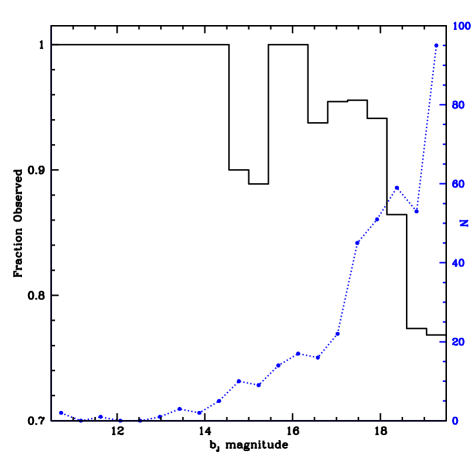
Figure 1: Fraction of galaxies from the parent APM catalogue that are selected for observation with 2dF (solid line histogram and left hand vertical axis) with the total number of galaxies available for selection (dotted line; right hand vertical axis).

Our observations used the 580V and 385R gratings which yield a central dispersion of 1.0 and 1.6 Å pixel^-1 respectively. These AAOmega spectra are generally superior in quality to the 2dFGRS survey (Colless et al. 2001) given both the higher spectral resolution and coverage of a wider wavelength range, and are generally well-able to yield secure redshifts despite the somewhat inclement observing conditions.

Our dataset was reduced with the 2dF data reduction pipeline in a standard manner (see www.aao.gov.au/2df/). This included a Laplacian Edge Detection step to reject cosmic rays from our data in an efficient manner (see Farage & Pimbblet 2005 and references therein for a full discussion of the benefits of this methodology). To obtain redshifts of our targets, we made use of the zcode package that was originally employed on 2dFGRS by Colless et al. (2001), and we refer the reader to that publication for more explicit details. The output of the code consists of a cross-correlation with the best-matched template spectra, i.e. those with the highest $R$ value according to Tonry & Davis (1979). Our template spectra range from G stars, through globular clusters, right out to galaxy spectra. Each redshifted target was then de-redshifted to rest-frame wavelengths and checked by eye (by KAP) to ensure that the emission and absorption features are in the correct locations. The fraction of our targets that produce reliable redshifts is high: 87 per cent of all our targets (100 per cent for $b_{J}<15.0$, only dropping below 80 per cent at $b_{J}>19.25$). We present our redshift catalogue in Appendix A.

3 Redshifts and Reliability Control

In total, we obtained redshifts for 307 objects. Of these, three are most likely stellar in nature as they have velocities of less than 200 km s^-1. One of them (PRA003) is SDSS J114948.77$-$014728.2, already suggested to be a star in the SDSS database (Abazajian et al. 2009), and two others (PRA096 and 244) had radial velocities measured in 2dFGRS suggesting them to be stars.

To further probe the reliability of our redshift measurements we proceed by comparing our redshifts to those already published in the literature. For this comparison, we make use of a number of other catalogues that possess an overlap with our own observations: 2dFGRS (Colless et al. 2003); 2QZ (Croom et al. 2004); 6dFGS (Jones et al. 2009); SDSS Data Release 7 (DR7; Abazajian et al. 2009); Da Costa et al. (1998); Doyle et al. (2005); Falco et al. (1999); Grogin et al. (1998); Quintana & Ramírez (1995); Shectman et al. (1996); Slinglend et al. (1998); & Theureau et al. (2004). In some cases, a target in our catalogue appears in several of the above catalogues, each with a different reported redshift. In Fig. 2, we plot the difference between our measured redshifts and the literature redshifts. The measured mean and median difference in redshift is $-$23 km s^-1 and 27 km s^-1, respectively. When performing this analysis, we found two especially note-worthy, low redshift, discrepancies between our redshifts and previously published ones, which exceed by far the quoted redshift errors. The first major difference is between ourselves and 6dFGS (PRA284; Appendix A) – this is due to a poor quality 6dFGS spectrum (D.H. Jones, priv. comm.).

Figure 2: Deviation of literature redshifts from our measured redshifts, including targets that have multiple matches to various different sources.

The second is PRA037 (also 2MASX J11481434$-$0159000; Appendix A) when compared to Quintana & Ramírez (1995). This galaxy also has published redshifts in three other catalogues. Whilst our redshift is non-discrepant with both 2dFGRS (Colless et al. 2003) and 6dF (Jones et al. 2009), it is $2.6\sigma$ away from that published in SDSS-DR2 (Abazajian et al. 2004). The reason for the discrepancy becomes more obvious from an examination of this object’s image at optical (i.e. the Digitized Sky Survey and SDSS) and NIR (i.e. 2MASS) wavelengths: it possesses a secondary core or neighbour galaxy 6 arcsec away at PA $\sim 230^{\circ}$. We therefore contend Quintana & Ramírez (1995) on the one hand, and SDSS-DR2, 2dFGRS, and 6dF on the other, each measured a different core’s velocity.

4 Analysis

4.1 Dynamics

We begin our analysis of the dynamics and architecture of A1386 by examining its velocity structure. In constructing the velocity histogram (Fig. 3), we include not only the objects from our new observations, but also all objects with redshifts available from the literature (see Section 3, above, and Appendix). Measurements that belong to the same galaxy were identified, based on their close positional coincidence, and the velocity with smallest error was chosen for that galaxy.

Figure 3: Velocity histogram for our observations combined with further velocities obtained from the literature. The upper panel of the figure displays an enlarged region from the lower panel. The velocity structure of field of A1386 is complex and likely comprises at least four sub-clusters or groups.

The velocity distribution (Fig. 3) is unusually broad, with several sub-peaks, and there appears to be rich and highly complex substructure in the core of A1386. The complexity is perhaps not unexpected given that A1386 resides within the supercluster Leo A (SCL100 in Einasto et al. 1997; cf. Pimbblet, Edge & Couch 2005) and hence is a part of the Sloan Great Wall (see Fig. 9 of Gott et al. 2005). We note that this broad peak in velocity is, however, distinct and isolated from other foreground and background structures. Indeed, this cluster is very isolated in redshift space: the closest cluster in redshift space is WBL 355 at $z\sim 0.028$ (White et al. 1999), some 52 arcmin due WNW from the centre of A1386. We refrain from making further analysis of WBL 355 as our observations are only just probing the outskirts of this poor cluster.

We note that the redshift of A1386 ($z=0.1018$) given by Struble & Rood (1999) is based on that of a single galaxy (published by Quintana & Ramírez 1995) whose redshift is coincidentally located near the middle of the velocity distribution. However, it presents a real problem in trying to compute any ‘mean’ redshift of the population, let alone a meaningful velocity dispersion (cf. Abell 779 in Oegerle & Hill 2001). This can readily be illustrated by a simple application of the $3\sigma_{v}$ clipping technique of Yahil & Vidal (1977) where the mean velocity and dispersion of a cluster are determined by iteratively clipping any galaxy that is greater than $3\sigma_{v}$ from the mean of the velocity distribution. Using an initial clip of 21000 km s${}^{-1}<cz<42000$ km s^-1, we obtain a mean velocity of $31241\pm 275$ km s^-1 and an unphysically large (and clearly erroneous) velocity dispersion of 5723 km s^-1. We are thus forced to split up the cluster into more sensibly sized sub-components. Fig. 3 would suggest that there are multiple sub-peaks in the overall velocity distribution and therefore we proceed with the aim of attempting to isolate these peaks.

4.2 Substructure

Based on an inspection of Fig. 3 it is likely that A1386 has at least four components (mean velocities of approximately 25000 km s^-1, 28500 km s^-1, 31000 km s^-1 and 37000 km s^-1; see Fig. 3) that make up what Abell (1958) originally defined as the cluster proper. In order to better delineate the structure of the cluster, we now apply the Dressler & Shectman (1988; DS) test to our catalogue – one of the most sensitive general tests for substructure available (Pinkney et al. 1996; see also Section 4.4). For each cluster member, the DS algorithm computes the mean local velocity, $\overline{cz}_{local}$, and local standard deviation, $\sigma_{local}$, of that member’s $N_{local}$ nearest neighbours in projection. These localized values are then compared to the global values of the cluster mean velocity, $\overline{cz}$, and cluster velocity standard deviation, $\sigma_{v}$, to produce a measure of deviation:

$$\delta^{2}=\left(\frac{N_{local}+1}{\sigma_{v}^{2}}\right)[(\overline{cz}_{local}-\overline{cz})^{2}+(\sigma_{local}-\sigma_{v})^{2}]$$ (1)

that can be utilized to locate clumps of spatially close deviant galaxies. Consistent with DS, in this work we use the 10 nearest neighbours (i.e. $N_{local}+1=11$) to compute $\delta$. A cumulative quantity, $\Delta$, is then found by summing all values of $\delta$ for the cluster. By comparing $\Delta$ to Monte Carlo simulations in which the member’s velocities are shuffled around the positions, we can estimate a confidence level for the overall probability of substructure in the cluster.

We acknowledge that we can already guess that the DS test will show that the cluster has substructure – the primary purpose of applying this technique, however, is to specify the sky positions of likely sub-components within the cluster. Figure 4 displays the results of applying the DS test to our data – each circle is drawn with a diameter proportional to the deviation of a given galaxy from the global mean velocity (here, assumed to be 31241 km s^-1), $e^{\delta}$ (see DS for full details of the test); hence substructure is interpreted as (spatially close) overlapping circles. We also display the results of the average and most deviant of 1000 Monte Carlo simulations in Fig. 4.

Figure 4: Results of the DS test. Top left: spatial distribution of all galaxies with $21000$ km s${}^{-1}<cz<42000$ km s^-1 . Top right: Result of the DS test as applied to A1386 – spatially close overlapping circles denote likely substructure locations. Bottom left: average of 1000 Monte Carlo simulations. Bottom right: the single most deviant of 1000 Monte Carlo simulations.

Unsurprisingly, the DS test gives unequivocal evidence for sub-clustering as the probability of obtaining the cumulative deviation found for the cluster is very low in comparison to the simulations: $P(\Delta)\ll 0.001$.

Interestingly, Fig. 4 displays several regions of overlapping circles in the real data suggesting localized sub-clustering (Dressler & Shectman 1988). We now ask if any of these regions (or, indeed, any localized regions at all) correspond to any of the individual peaks seen in redshift space (Fig. 3). To do this, we split the cluster catalogue up into six redshift channels that encompass each of the major peaks seen in Fig. 3 and search (by eye) for any obvious spatial overdensities. The result of this search is depicted in Fig. 5.

       

       

       

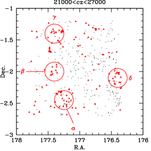
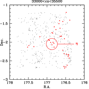
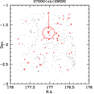
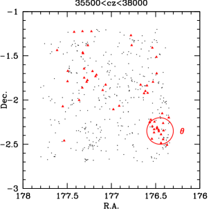
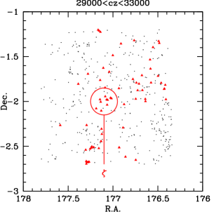
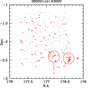
Figure 5: Spatial distribution of galaxies in redshift channels corresponding to the peaks seen in Fig. 3 (triangles); all other galaxies in the range $21000$ km s${}^{-1}<cz<42000$ km s^-1 are plotted as dots. Localized overdensities – i.e. likely cluster sub-components – are circled and labelled $\alpha$ through $\kappa$.

We believe that the sub-component marked $\zeta$ is the cluster proper because it is nearest to what Abell (1958) catalogued as the cluster centre. Comparing Fig. 5 to Fig. 4 shows that a number of the other sub-components (e.g. $\delta$) probably constitute sub-clusters that are interacting in a complex manner with $\zeta$, and potentially with each other as well.

Of the other overdensities, we suggest that $\theta$ and $\kappa$ are the same entity that extends over two of the redshift channels in Fig. 5. We identify $\theta$ and $\kappa$ as Abell 1373. By limiting the redshift distribution to the range $35500<cz<42000$kms^-1 and localizing the spatial extent to $176.3^{\circ}<RA<176.6^{\circ}$ and $-2.6^{\circ}<Dec<-2.3^{\circ}$, we compute that Abell 1373 has a mean velocity of $38063\pm 256$ kms^-1 and a velocity dispersion of $1428^{+228}_{-154}$ kms^-1 from 31 members. Our values for $\overline{cz}$ and $\sigma_{v}$ are comparable (i.e. within $3\sigma$) to those computed in the recent study of rotating galaxy clusters by Hwang & Lee (2007) despite using a different spatial extent.

We have also searched the NASA/IPAC Extragalactic Database (NED, nedwww.ipac.caltech.edu) for possible clusters that may correspond to overdensities $\alpha$ through $\kappa$ in order to check whether they were known before. We found reasonable matches with clusters reported by Estrada et al. 2007; Koester et al. 2007; Miller et al. 2005; and Merchán & Zandivarez 2002, and present these in Table 1, along with basic data on the overdensities themselves.

We have approximated the mean velocity of each group by taking all galaxies within the marked circles (radius of 0.15^∘ on the sky; equivalently 1 Mpc at $z=0.1$) in Fig 5 for the purpose of matching them to the literature. We will refine these values later in this work by undertaking detailed decomposition work using Kaye’s Mixture Model. We note that a number of our groups have reasonable matches to known literature clusters ($\alpha$, $\delta$, $\zeta$, $\theta$ & $\kappa$). A further two matches ($\epsilon$ & $\eta$) are found within the MaxBCG catalogue of Koester et al. (2007). Although the MaxBCG photometric cluster redshifts are not quite the same as our spectroscopic cluster redshifts, they are of the order of the quoted photometric redshift error of $\Delta_{Z}=0.01$ given by Koester et al. (2007) away from our estimates. Therefore we regard these matches as plausible. Finally, $\theta$ is identified as matching EAD2007 236 (Estrada et al. 2007) which is also based on a photometric redshift. We suggest that EAD2007 236 may be a foreground extension to A1373.

Table 1: Known clusters in the literature with close proximity to the overdensities identified in Fig 5. The mean velocity quoted for each group is computed from galaxies within the marked circles (radius of 0.15^∘) in Fig 5.

Group	RA (J2000)	Dec (J2000)	$\overline{cz}/$ km s-1	NED Match	RA(NED)	Dec(NED)	cz(NED)
$\alpha$	11 49 00	$-$02 22 36	26083	SDSS-C4 1121	11 48 51	$-$02 30 37	26235
$\beta$	11 49 38	$-$01 59 24	23675	No plausible match found
$\gamma$	11 49 36	$-$01 24 00	25177	No plausible match found
$\delta$	11 45 36	$-$02 06 00	24343	MZ 07066	11 45 29	$-$02 06 24	23769
$\epsilon$	11 48 05	$-$01 42 00	28243	MaxBCG J177.02469-01.68868	11 48 06	$-$01 41 19	32393†
$\zeta$	11 48 22	$-$02 00 00	30813	Abell 1386	11 48 22	$-$01 56 41	30519
$\eta$	11 47 31	$-$02 01 48	34408	MaxBCG J176.79744-01.88906‡	11 47 11	$-$01 53 21	30774†
$\theta$	11 45 46	$-$02 19 48	36326	[EAD2007] 236	11 45 52	$-$02 20 11	34704†
$\iota$	11 47 12	$-$02 24 00	38975	No plausible match found
$\kappa$	11 45 31	$-$02 28 12	39092	Abell 1373	11 45 28	$-$02 23 40	39393
† Denotes a photometric cluster redshift estimate.
‡ It is possible that $\eta$ is a SW extension of $\epsilon$.

4.3 Brightest Cluster Members

If the sub-components identified in Fig. 5 truly are sub-clusters or groups, then when we examine each separately, they may visually resemble such a group. For instance, each sub-component may contain a brightest cluster member (BCM) that is a giant elliptical or a cD class galaxy with an extended diffuse halo; or we may find several galaxies in the act of merging to form such a galaxy surrounded by an overdensity of early-type galaxies (cf. Bautz & Morgan 1970). Conversely, not finding a cD class galaxy does not immediately mean that we have not located a cluster. The majority of Abell clusters are of “late” Bautz-Morgan type, i.e. they lack an obvious central, bright and dominant early-type galaxy; here, we are aiming to build up a body of evidence for the most probable sub-groups.

In order to perform this test, we inspect SDSS images of the regions centred on the sub-components. Out of the components identified in Fig. 5, we find that groups $\alpha$, $\gamma$, $\delta$, $\epsilon$ and $\zeta$ have obvious bright ellipticals within the regions indicated in Fig. 5. Of these, $\alpha$, $\delta$, $\epsilon$ and $\zeta$ are all at the correct redshift but the bright elliptical near the $\gamma$ spatial overdensity is a foreground object. We display these four BCMs in Fig. 6.

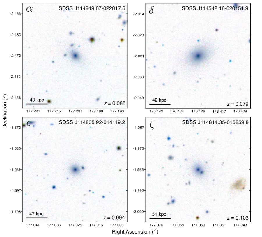
Figure 6: BCMs in the groups identified in Fig. 5. All of them have the correct redshifts to be associated with the groups that they were identified from.

The BCM in $\alpha$ is SDSS J114849.67$-$022817.6 and was not observed in our sample due to fibre collisions and prioritization at the field configuration stage (the same is true for $\delta$ and $\epsilon$). The redshift of this galaxy from SDSS is $cz=25428$ km s^-1. We identify the BCMs in $\delta$ and $\epsilon$ as SDSS J114542.16$-$020151.9 ($cz=23624$ km s^-1) and SDSS J114805.92$-$014119.2 ($cz=28181$ km s^-1) respectively. Meanwhile, PRA037 is identified as the BCM of $\zeta$, and SDSS J114814.35$-$015859.8 (also labeled 2MASX J11481434-0159000), with $cz=31022$ km s^-1 from our catalogue.

4.4 Results of the KMM algorithm

The DS test is one of the best tests available in a generic three dimensional case for finding substructure (Pinkney et al. 1996). It is not, however, without its own problems. Although it can be readily sensitive from equal mass mergers down to a 3:1 mass merger ratio given modest numbers of redshifts (cf. Pinkney et al. 1996; Pimbblet 2008), the number of false positive detections can pose problems. Indeed, it may be that some of the sub-components outlined above do not represent true infalling groups or sub-clusters (e.g. $\beta$; see Fig. 5) given their lack of bright ellipticals. Moreover, false positive detections can be particularly evident for clusters that have features such as significant radial gradients in their velocity dispersion profiles (Pinkney et al. 1996). With a structure such as A1386, the likelihood of false positives may be comparatively high.

To proceed further with delineating the possible sub-components, we now apply Kaye’s mixture model (KMM) algorithm to the velocity distribution. The KMM algorithm is described in detail in Ashman et al. (1994) and has been used extensively in the literature (e.g. recent examples include Owers et al. 2009; Johnston-Hollitt et al. 2008) for just this purpose. In brief, based on a user-supplied number of Gaussians with some initial best guess of their central position, the KMM algorithm effectively partitions the data into a number of sets and evaluates whether the fit that results from these Gaussians is superior to a single Gaussian fit. In all cases studied in this work, multiple Gaussians are always found to be superior fits to the data than a single Gaussian by the KMM algorithm. The key questions here are what input should the KMM be given: how many Gaussians should one fit to the data and with what initial parameters?

In the one-dimensional case, we elect to try two sets of parameters: the first with four Gaussians and the second with six. The reason for these choices stems from visual inspection of Fig. 3 as discussed above. For each peak in the velocity distribution, we use an approximate guess of the velocity dispersion ($\sigma_{v}$) from a visual inspection of Fig. 3. We present the input and output parameters for these two scenarios in Table 2.

We conducted several runs of the KMM algorithm to check how sensitive the results are to the initial conditions imposed by guessing the Gaussian’s parameters (i.e. $\sigma_{v}$ and $\overline{cz}$). This was done by perturbing both $\sigma_{v}$ and $\overline{cz}$ by incremental amounts. In the cases where the perturbation is modest ($\Delta(\overline{cz})<500$ km s^-1 and $\Delta\sigma_{v}<0.5\sigma_{v}$), the KMM algorithm converged on the same solution. Therefore, despite guessing the initial inputs, we regard the output of the KMM algorithm to be reasonably robust.

From Table 2, it appears that a four-Gaussian approach is incorrect. The highest-redshift Gaussian (labelled group 4 in Table 2) of the four-Gaussian approach has a very large velocity dispersion of $\sigma_{v}=2316$ km s^-1. We regard this as erroneous since the implied cluster mass would be unphysically high. However, the first three Gaussians are good fits to the data and are highly plausible.

The six-Gaussian solution appears to be superior to the four-Gaussian solution at first glance (Table 2). Effectively, what was group 4 in the four-Gaussian solution has been segmented into three new sub-components. Of these, group 4 looks to be nearly perfectly partitioned, with groups 5 and 6 both possessing more reasonable parameters than before. Arguably, we could also partition group 6 into two further sub-components (centred on $\approx$ 38000 and $\approx$ 40000 km s^-1). But doing so results in very few galaxies ($N_{gal}=19$) in one partition and a much reduced correct allocation rate (76 per cent) indicated by the KMM algorithm. Hence we do not regard seven Gaussians as an improvement over the six-Gaussian solution in one dimension.

Table 2: Input and output parameters for the one-dimensional application of the KMM algorithm. The table is split into two halves: the upper half shows the result of inputting four Gaussians to the KMM algorithm, whereas the bottom half shows the result of six Gaussians. The final column shows an estimate of the correct allocation rate by KMM for each partition.

	Input Parameters		KMM Output
Group	$\overline{cz}/$ km s-1	$\sigma_{v}/$ km s-1	$\overline{cz}/$ km s-1	$\sigma_{v}/$ km s-1	$N_{gal}$	Rate ($\%$)
1	25000	1000	24807	1161	138	98
2	28500	500	28219	451	56	99
3	31000	750	30856	818	66	98
4	37000	2000	37398	2316	173	98
	Input Parameters		KMM Output
Group	$\overline{cz}/$ km s-1	$\sigma_{v}/$ km s-1	$\overline{cz}/$ km s-1	$\sigma_{v}/$ km s-1	$N_{gal}$	Rate ($\%$)
1	25000	1000	24807	1161	138	98
2	28500	500	28219	451	56	99
3	31000	750	30856	818	66	98
4	34500	500	34507	548	39	98
5	37000	500	36560	452	49	97
6	39500	1000	39442	1022	85	98

4.5 Interpretation

Taken together, the above suggests that the galaxy populations of these other clusters have biased the cluster and richness identification made by Abell (1958). There are at least three significant, bona-fide sub-clusters in the field of A1386: these are the first three redshift slices specified in Table 2 (both the four and six Gaussian KMM solutions).

Of these, the second and third groupings are fairly solid detections with a single BCM each ($\epsilon$ and $\zeta$; Figs. 5 and 6). The first cluster in Table 2 merits further attention given it has two sub-clusters ($\alpha$ and $\delta$; Fig. 6) with potential BCMs (Fig. 6), both of which have matches to literature clusters (Table 1). On the face of it, this first sub-cluster appears to have a velocity dispersion ($\sigma_{v}=1088$ km s^-1) that is typical of a rich, massive galaxy cluster by itself. But given the two BCMs and their spatial separation (Fig. 5; $\approx 2.5$ Abell radii apart), it may be the case that this redshift grouping is a cluster that is undergoing the early to mid-stages of a merger event.

To test this hypothesis, we apply a further DS test, but limit ourselves to only those galaxies contained in the first redshift grouping in Table 2. Given we have 138 galaxies in this redshift slice, we will be sensitive to about a 4:1 mass merger ratio (see Pinkney et al. 1996). The DS test for this redshift slice generates a result of $P(\Delta)\ll 0.001$ which strongly suggests the presence of substructure.

Figure 7: DS test results of the first redshift peak identified in Table 2. The cross denotes the position assigned to A1386 by Abell (1958). Two major sub-clusters which contain BCMs ($\alpha$ and $\delta$) can be seen at (RA,Dec)=(177.3,$-$2.5) and (176.4,$-$2.1). We suggest that these are two clusters or groups in their own right.

In Fig. 7, we show the results of the DS test in this redshift slice. From this, it is quite clear that there are two major self-contained sub-clusters (RA,Dec)=(177.3,$-$2.5) and (176.4,$-$2.1) that dominate this slice. Moreover, these two sub-clusters, $\alpha$ and $\delta$, are among those in which we identified typical BCMs. It may also be the case that the $\beta$ and $\gamma$ groups (Fig. 5) are groups in their own right as well, but we have not been able to identify dominant BCMs in these regions and they are probably false positives given the small number of redshifts available (cf. Pinkney et al. 1996).

The six-Gaussian solution to the KMM algorithm (lower half of Table 2) suggests that the three slices with the highest redshift may also contain groups or clusters of galaxies in their own right (indeed, we have already identified A1373 at 38063 kms^-1; see above). However, apart from A1373, the lack of BCMs coupled with no high galaxy overdensity suggests otherwise. The simplest interpretation for these three redshift slices is that they are part of some larger-scale structure. Indeed, looking at the $cz>38000$ km s^-1 slice in Fig. 5 (which approximately corresponds with the highest redshift slice in Table 2) the galaxies appear to be spread across the sky in the same manner that walls and filaments of galaxies are (cf. Pimbblet et al. 2005).

To summarize, we present the global parameters for the four groupings that we contend are bona-fide clusters in their own right in Table 3 from all of the above analysis. We estimate errors for $\sigma_{v}$ following Danese et al. (1980). For the clusters that we name A1386-A and -B, we restrict our computation of $\overline{cz}$ and $\sigma_{v}$ to the area of overlapping circles suggested by Fig. 7 (i.e. coarsely splitting the $21000$–$27000$ kms^-1 redshift slice at R.A.$=177$ and Dec.$<-1.9$) and apply the clipping technique of Zabludoff et al. (1990). For A1386-C and -D, we use all available redshifts in the appropriate redshift slice (Figure 5) over the full field of view (unlike for A1386-A and -B) and apply the same redshift clipping technique. We also note that the clusters in Table 3 extend beyond an Abell radius from the original Abell (1958) definition of A1386 – this is apparent in the case of A1386-A where A1373 is the closest companion in projection.

Table 3: Bona-fide clusters and groups with dominant BCMs in the field of A1386. N(gal) is the number of galaxies used to derive $\overline{cz}$ and $\sigma_{v}$ and covers the whole field of view for A1386-C and -D, but is spatially limited to the area of the subclusters found in Fig. 7 for A1386-A and -B.

Name	N(gal)	$\overline{cz}$	$\sigma_{v}/$	Other Cluster Names	BCM	$v_{pec}$	$v_{pec}/\sigma_{v}$
		(km s-1)	(km s-1)		(km s-1)
A1386-A	21	$23593\pm 68$	$310^{+64}_{-39}$	MZ 07066	SDSS J114542.16$-$020151.9 ($\delta$)	$-$95	$-$0.43
A1386-B	32	$25952\pm 83$	$482^{+73}_{-50}$	SDSS-C4 1121	SDSS J114849.67$-$022817.6 ($\alpha$)	$-$297	$-$0.88
A1386-C	56	$28219\pm 70$	$451^{+60}_{-42}$	MaxBCG J177.02469-01.68868	SDSS J114805.92$-$014119.2 ($\epsilon$)	$-$61	$-$0.15
A1386-D	66	$30856\pm 99$	$818^{+81}_{-63}$	Abell 1386	SDSS J114814.35$-$015859.8 ($\zeta$; PRA037)	$+$108	$+$0.15

Since our main, long-term aim in assembling these observations was to look more closely at peculiar velocities of BCMs (cf. Coziol et al. 2009; Pimbblet 2008; Pimbblet et al. 2006), we also compute the peculiar velocity, $v_{pec}=(v_{BCG}-\bar{v}_{cluster})/(1+z)$, for each group in Table 3. Following Coziol et al. (2009), we express these results as a fraction of the velocity dispersion, i.e. $v_{pec}/\sigma_{v}$, to determine their level of significance (Table 3).

Two of the clusters in Table 3 have BCM peculiar velocities that are small fractions of the cluster velocity dispersions: A1386-C is $-0.15\sigma_{v}$ away from $\overline{cz}$; and A1386-D is $0.15\sigma_{v}$.

Meanwhile, A1386-B is $-$0.88$\sigma_{v}$ away from $\overline{cz}$ and A1386-A’s BCM is $-$0.43$\sigma_{v}$ away from $\overline{cz}$. These values are large fractions of the velocity dispersion (see Section 3.2 of Coziol et al. 2009 for a full discussion of this parameter) and may be interesting groups for further observation. These peculiar velocity results are also in contrast to the values obtained by Coziol et al. (2009). This is largely due to the careful investigation of the A1386’s substructure that we have undertaken in this work and suggests that future investigation of BCG peculiar velocities, especially in complex areas as this one, must be undertaken with equal care in order to avoid erroneous outcomes.

As a final validation of these four groupings (Table 3), we construct colour-magnitude diagrams for them and check whether we can see a defined colour-magnitude relation (e.g. Visvanathan & Sandage 1977; Bower, Lucey & Ellis 1992). This is achieved by extracting SDSS ($g-r$) colours around the BCM of each group (Table 3) to a radius of 0.5^∘ within $3\sigma_{v}$ of the mean velocity given in Table 3 and comparing the location of any obvious early-type ridge line with the empirical predictions of López-Cruz, Barkhouse & Yee (2004; in particular see the equations contained in Figs. 3 and 4 of that work) who surveyed clusters over a comparable redshift range to the present work. One immediate issue in performing this analysis is that the equations presented by López-Cruz et al. (2004) are in the Kron-Cousins system (calibrated to Landolt 1992 standards), rather than SDSS $ugriz$ photometry. Hence we transform the SDSS photometry to Kron-Cousins using the transformations derived by Lupton. Although Lupton derived these transformations for stellar objects, these transforms should hold for galaxies that do not have significant emission lines – just as one would expect for galaxies around the colour-magnitude relation.

The resultant colour-magnitude diagrams are shown in Fig. 8 along with the López-Cruz et al. (2004) prediction for the early-type ridge line. All of the four groupings show galaxies that are consistent with the predictions of where the ridge line should lie (especially given the errors inherent in the photometric conversion to Kron-Cousins and the errors of the line given by López-Cruz et al. 2004; especially the scatter observed in Fig. 4 of López-Cruz et al. 2004). Therefore we conclude that the field of A1386 is made up of at least four sub-units along the line of sight, and possibly a few filaments as well, at the high redshift end of the distribution seen in Fig. 3. We emphasize our observations and analysis of A1386 is wider than an Abell radius at these redshifts and therefore encompasses an area that Abell (1958) may not have examined in great detail. In passing, we note that A1386-B seems to have a modest blue fraction of galaxies (e.g., Butcher & Oemler 1984) indicating that it is more highly star-forming than the other clusters we have detailed.

Figure 8: Colour-magnitude diagrams for the groups identified in Table 3. The early-type ridge line is the empirical relation found by López-Cruz et al. (2004). Each group has galaxies that are consistent with this relation, therefore adding weight to the finding that these groups are real.

5 Sloan Great Wall

A1386 does not reside in just any part of the sky: it is a part of the Leo A supercluster (Einasto et al. 1997) and hence is a part of the Sloan Great Wall (SGW; Gott et al. 2005; Nichol et al. 2006; Deng et al. 2007; Einasto et al. 2010). Although the SGW ‘may be the largest coherent structure yet observed’ (Tegmark et al. 2004) in the Universe, it could have still plausibly been formed from random phase Gaussian fluctuations (see Tegmark et al. 2004; Gott et al. 2005) and even larger structures may yet be found (Shandarin 2009).

In Fig. 9 we demonstrate how our new radial velocities fit in with the SDSS measured velocities in the region of the SGW. Our new measurements are probing the central regions of the SGW, at RA$\sim$11.8 hr. This region of the SGW is where it has split into two defined filaments that stretch from $\sim 11.3$ hr to $\sim 12.7$ hr (cf. Fig. 9 of Gott et al. 2005).

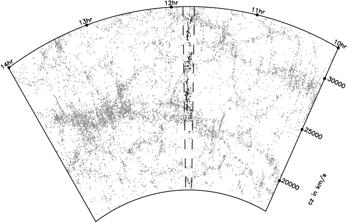
Figure 9: Our new observations of A1386 combined with all available literature redshifts (black dots) plotted in the context of the Sloan Great Wall (SDSS data shown as grey dots in the declination range of $1.5^{\circ}<\delta<-3.5^{\circ}$). The dashed lines denote the spatial extent of our AAOmega observations. A1386 sits near the heart of the Great Wall in right ascension terms.

The first point to make is that our new observations probe both the median $cz$ range of the SGW and beyond. At A1386’s declination, we qualitatively appear to be estabishing a previously hinted line-of-sight filament (Fig. 9). This can readily be seen by contrasting the redshift histogram (Fig. 3) with the points delineated by the dashed lines in Fig. 9 which denote the right ascension extent of our observations.

Our observations also better define the split in the SWG with higher fidelity than previous works. Indeed, A1386-A resides at almost the Western end of this split, with A1386-B residing beyond the two main filaments of the SGW. Given the difference in $cz$ between A1386-B (Table 3) and the bulk of the Great Wall, we suggest that the interpretation is that this component A1386-B is likely to be infalling along the line of sight to the ‘bulk’ of the Great Wall at $cz\sim 24000$ km s^-1.

This raises the question as to whether any or all of the four groups that we have identified (Table 3) are interacting with each other. The difference in recession velocity between the groups is: $\Delta_{AtoB}=2359$ km s^-1; $\Delta_{BtoC}=2267$ km s^-1; $\Delta_{CtoD}=2637$ km s^-1. Given the small velocity dispersion of both A1386-A and A1386-B, it is unlikely that these two groups are interacting. $\Delta_{BtoC}$ is more than 5 times the velocity disperion of A1386-C ($\sigma_{v}=451$km s^-1), thus A1386-C is also unlikely to be interacting with A1386-B. Even $\Delta_{CtoD}$ is at least $>3.5\sigma_{v}$ of A1386-D. Hence we believe that these groups and clusters are probably not interacting with each other, although they may be moving coherently toward the bulk of the Great Wall. However, the analysis above does not preclude the possibility that the groups found in the present work are connected by filaments extending in a radial direction (cf. Lu et al. 2010) which could be verified with a deeper and more complete spectroscopic sample. Indeed, Fig. 9 displays hints that all of our groups may be in proximity to larger filaments (cf. Pimbblet et al. 2004).

6 Summary

This work has presented a catalogue of three hundred radial velocities (78 of them new) in the direction of A1386 as part of our on-going endeavours to identify peculiar velocities of BCMs in Abell clusters. Here, we have taken a critical examination of A1386 to unravel its complex architecture and its place in the large-scale structure around it by looking at its relationship with the Sloan Great Wall.

We have demonstrated that A1386 is a not a simple, relaxed galaxy cluster. It is composed of at least four separate clusters, perhaps more, along the line of sight that are spatially close to one another on the sky. We have delineated these structures through a combination of statistical substructure tests, presence of a dominant BCM, and colour-magnitude relations. The global parameters for these new clusters are given in Table 3. Of these, A1386-A and A1386-B both have a BCM with a peculiar velocity that is a large fraction of their velocity dispersions. Our results are in contrast to the results of Coziol et al. (2009), who report different subclusters, and therefore different peculiar velocities. The only common subcluster between our two works is A1386A (as per Coziol et al. 2009), which in our work has been divided in to A1386-C and A1386-D (Table 3).

There are several walls or filaments of galaxies that pass through the line of sight to A1386. These are seen in Fig. 3 as peaks at $cz>33000$ km s^-1. A1386 is also located near the heart of the Sloan Great Wall. Of the sub-clusters identified, we suggest that only A1386-A is associated with the SGW itself. Although the other newly identified clusters may be moving toward other mass concentrations (both in and beyond the SGW), we suggest that at this time the other clusters are not physically bound to the SGW and none of them are interacting with one another significantly.

Appendix A Redshift catalogue

In Table A1, we present the new radial velocities we measured from our AAOmega observations. The designation ‘PRA’ that appears in the table refers to three of the authors of this work (KAP, IGR & HA) who created the original telescope time application, the target list and reduced the dataset.

Table 4: The redshift catalogue. The $R$ magnitude is sourced directly from the APM catalogue. Where applicable, we have listed our targets that also appear in other catalogues (right hand columns). The sources for these are codified as follows: (a) 2dFGRS (Colless et al. 2003); (b) 6dFGS (Jones et al. 2009); (c) HIPASS (Doyle et al. 2005); (d) Quintana & Ramírez (1995); (e) LCRS (Shectman et al. 1996); (f) UZC (Falco et al. 1999); (g) SDSS-DR7 (Abazajian et al. 2009); (h) Slinglend et al. (1998); (i) Grogin et al. (1998); (j) Da Costa L.N., et al. 1998.

						Other Measurements
Identification	RA	Dec	$R$	$cz_{helio}$	$\Delta cz$	$cz_{helio}$	$\Delta cz$
Tag	(J2000)	(J2000)		(km s-1)	(km s-1)	(km s-1)	(km s-1)	Source
PRA001	11 49 42.44	$-$02 02 13.8	18.28	24720	101	24724	42	g
PRA002	11 49 46.56	$-$02 00 19.5	17.28	25527	128	25422	64	a
						25347	49	g
PRA003	11 49 48.83	$-$01 47 27.2	15.64	26	29
PRA004	11 50 41.87	$-$01 59 21.8	17.02	40714	110	40625	52	g
PRA005	11 49 30.61	$-$01 58 54.8	19.32	25545	20
PRA006	11 51 07.80	$-$02 02 13.2	17.86	18161	74	17988	89	a
						18072	48	g
PRA007	11 50 53.60	$-$02 03 07.4	19.22	80293	116
PRA008	11 49 25.68	$-$02 01 19.7	16.75	25287	20	25237	43	g
PRA009	11 49 56.40	$-$02 05 23.8	16.63	34239	23	34188	42	g
PRA010	11 50 46.70	$-$02 01 47.8	19.18	48677	23	48536	123	a
PRA011	11 50 12.00	$-$02 04 19.2	19.46	37360	20
PRA012	11 51 11.97	$-$02 05 31.7	17.25	48755	23	48776	64	a
						48773	46	g
PRA013	11 50 10.33	$-$02 06 59.0	19.37	57800	23
PRA014	11 50 32.79	$-$02 06 17.0	17.81	46911	23	46768	64	a
						46777	53	g
PRA015	11 50 04.83	$-$02 07 56.2	19.13	34386	23	34326	89	a
PRA016	11 49 46.28	$-$02 02 58.6	18.62	25125	23	25123	89	a
PRA017	11 51 10.20	$-$02 07 00.5	19.14	67045	23	66914	89	a
PRA018	11 50 05.65	$-$02 12 51.8	18.15	26450	20	26382	89	a
PRA019	11 50 33.54	$-$02 13 35.3	17.93	40630	20	40592	64	a
						40550	51	g
PRA020	11 48 31.06	$-$02 02 40.5	13.62	8493	17	8424	89	a
						8502	28	g
PRA021	11 48 59.41	$-$02 00 31.0	15.92	8553	17	8574	64	a
						8544	89	b
						8574	27	g
PRA022	11 49 33.56	$-$02 04 36.8	18.92	43434	20	43500	89	a
PRA023	11 50 26.64	$-$02 10 18.4	16.21	18044	20	18027	23	g
PRA024	11 48 08.66	$-$02 07 46.9	18.96	44822	29
PRA025	11 48 32.97	$-$02 00 18.5	17.75	30932	20	30930	25	g
PRA026	11 48 50.40	$-$02 01 56.0	10.93	1711	17	1704	45	b
						1732	5	c
						1736	100	f
						1712	3	g
PRA027	11 50 21.18	$-$02 15 54.0	19.05	31972	20	31898	89	a
PRA028	11 48 27.65	$-$02 05 22.1	19.49	72507	23
PRA029	11 50 43.13	$-$02 16 59.9	17.94	25533	131	25243	64	a
						25288	45	g
PRA030	11 50 14.01	$-$02 28 07.3	16.80	27775	20	27761	64	a
						27794	27	g
PRA031	11 50 00.94	$-$02 21 33.7	19.06	49753	29	49766	89	a
PRA032	11 50 22.69	$-$02 14 39.4	18.21	23320	23	23324	89	a
PRA033	11 50 48.19	$-$02 28 27.6	18.24	25239	20	25273	89	a
PRA034	11 51 11.36	$-$02 38 28.9	19.03	25266	23
PRA035	11 50 32.03	$-$02 37 10.6	14.22	27760	20	27581	64	a
						27629	64	e
						27632	58	g
PRA036	11 50 59.91	$-$02 40 51.7	19.29	54607	26
PRA037	11 48 14.35	$-$01 58 59.8	14.66	31022	23	30849	89	a
						30930	45	b
						30655	93	d,1
						30945	55	g

Table 1: continued.

						Other Measurements
Identification	RA	Dec	$R$	$cz_{helio}$	$\Delta cz$	$cz_{helio}$	$\Delta cz$
Tag	(J2000)	(J2000)		(km s-1)	(km s-1)	(km s-1)	(km s-1)	Source
PRA038	11 48 40.15	$-$02 16 36.9	15.57	25482	20	25452	64	a
						25440	39	g
PRA039	11 48 35.99	$-$02 19 23.0	19.05	39287	20	39273	123	a
PRA040	11 49 29.08	$-$02 20 46.2	18.77	26294	29
PRA041	11 49 24.16	$-$02 21 24.8	18.29	25851	20	25572	89	a
PRA042	11 49 32.87	$-$02 28 48.5	15.99	26471	20	26262	89	a
						26385	28	g
PRA043	11 49 02.34	$-$02 21 40.9	17.85	27404	20	27221	89	a
						27398	28	g
PRA044	11 50 23.07	$-$02 41 19.6	19.21	13433	20	13461	64	a
PRA045	11 48 49.84	$-$02 22 34.8	17.11	26618	20	26592	89	a
						26709	54	g
PRA046	11 49 34.88	$-$02 20 49.1	18.98	39326	20	39363	89	a
PRA047	11 48 59.85	$-$02 27 21.9	18.13	26114	119	26142	89	a
						26028	48	g
PRA048	11 48 57.70	$-$02 31 00.4	17.25	30348	20	30099	89	a
						30264	41	g
PRA049	11 49 02.47	$-$02 32 55.4	18.57	25980	110	25962	64	a
						26109	44	g
PRA050	11 49 12.96	$-$02 19 20.1	17.31	26420	20	26622	64	a
						26502	52	g
PRA051	11 48 59.36	$-$02 30 22.0	16.90	27865	20	27911	89	a
						27827	48	g
PRA052	11 48 56.75	$-$02 31 53.9	15.07	17945	20	17928	89	a
						17961	51	g
PRA053	11 48 50.17	$-$02 31 44.4	18.98	25446	65	25542	64	a
PRA054	11 49 10.53	$-$02 15 49.9	18.33	30437	20	30609	123	a
PRA055	11 49 11.61	$-$02 39 57.7	15.68	30551	68	30429	64	a
						30532	45	b
						30471	45	g
						30523	43	e
PRA056	11 49 05.91	$-$02 25 35.1	17.04	25755	89	25782	64	a
						25758	46	g
PRA057	11 48 44.88	$-$02 04 43.9	17.43	30878	20	30879	64	a
						30903	38	g
PRA058	11 49 18.38	$-$02 34 20.5	17.58	27224	20	27311	89	a
						27202	70	e
						27212	30	g
PRA059	11 49 18.93	$-$02 18 35.4	16.98	26246	125	26262	64	a
						26229	50	g
PRA060	11 49 06.23	$-$02 40 38.7	16.84	30168	20	30200	55	e
						30207	25	g
PRA061	11 47 28.42	$-$02 04 09.0	18.36	34398	119	34206	64	a
						34314	45	g
PRA062	11 47 30.14	$-$02 01 53.3	19.35	30740	23
PRA063	11 49 12.85	$-$02 32 20.4	19.18	30812	20	30549	89	a
PRA064	11 49 09.37	$-$02 18 28.0	14.63	26618	20	26592	64	a
						26619	51	g
PRA065	11 47 26.57	$-$02 05 36.4	19.05	47736	23	47877	89	a
PRA066	11 48 41.50	$-$02 28 54.5	18.37	25440	20	25392	89	a
						25377	51	g
PRA067	11 48 46.73	$-$02 30 50.9	19.40	39314	20
PRA068	11 49 03.81	$-$02 40 23.0	17.77	30381	20	30429	64	a
						30432	30	g
PRA069	11 47 34.66	$-$02 08 20.9	17.92	17594	20	17598	89	a
PRA070	11 48 30.63	$-$02 18 20.2	17.72	30476	20	30399	64	a
						30468	30	g
PRA071	11 48 48.88	$-$02 40 52.3	18.57	25308	65	25123	89	a
						25285	49	g
						25331	58	e
PRA072	11 47 41.38	$-$01 58 41.5	18.63	93100	26

Table 1: continued.

						Other Measurements
Identification	RA	Dec	$R$	$cz_{helio}$	$\Delta cz$	$cz_{helio}$	$\Delta cz$
Tag	(J2000)	(J2000)		(km s-1)	(km s-1)	(km s-1)	(km s-1)	Source
PRA073	11 48 34.06	$-$02 27 40.4	17.93	25653	20	25482	89	a
PRA074	11 47 54.72	$-$02 06 18.9	16.90	36790	20	36665	64	a
						36758	16	g
PRA075	11 48 40.42	$-$02 25 29.4	17.35	25353	23	25333	89	a
						25419	52	g
PRA076	11 48 28.43	$-$02 25 22.4	17.84	39434	62	39303	89	a
						39381	42	g
PRA077	11 47 39.86	$-$02 23 42.8	17.26	38961	53
PRA078	11 47 44.69	$-$02 24 19.1	19.42	50691	56
PRA079	11 47 43.02	$-$02 15 23.8	18.16	39140	23	39243	89	a
PRA080	11 47 45.13	$-$01 57 06.5	15.82	34455	74	34386	123	a
						34356	47	g
PRA081	11 48 13.57	$-$02 36 38.8	17.95	46045	80	45868	64	a
						45961	49	g
PRA082	11 47 43.39	$-$02 30 48.9	19.19	31160	20
PRA083	11 48 32.03	$-$02 26 36.2	18.47	30662	68	30339	89	a
						30456	43	g
PRA084	11 48 04.48	$-$02 06 04.1	17.04	39827	23	39633	89	a
						39947	48	g
PRA085	11 47 43.13	$-$02 33 47.7	17.30	23021	26	22994	64	a
						23027	25	g
PRA086	11 48 10.60	$-$01 59 21.0	14.07	1555	17	1499	64	a
						1529	5	g
PRA087	11 48 27.35	$-$02 20 29.3	18.30	25821	20	25692	89	a
PRA088	11 48 04.11	$-$01 57 59.0	18.13	31112	71	31089	64	a
						31142	38	g
PRA089	11 47 29.72	$-$02 17 40.5	17.61	39116	65	38982	46	g
PRA090	11 47 22.46	$-$02 26 23.1	15.46	38445	20	38353	48	g
						38463	64	a
PRA091	11 47 17.24	$-$02 23 35.5	19.35	39581	110
PRA092	11 48 29.70	$-$02 21 48.8	17.82	30461	20	30549	89	a
						30498	51	g
PRA093	11 47 33.03	$-$02 17 32.1	19.10	29835	122	29859	89	a
PRA094	11 47 26.73	$-$02 36 59.2	15.03	29628	95	29671	46	g
PRA095	11 47 40.98	$-$02 35 28.8	17.59	52562	89	52494	64	a
						52383	58	g
PRA096	11 47 23.25	$-$02 22 31.9	18.11	$-$44	83
PRA097	11 47 06.08	$-$02 36 48.5	18.85	58513	23
PRA098	11 47 35.13	$-$02 20 45.5	18.95	38535	20	38523	64	a
PRA099	11 47 41.58	$-$02 32 57.4	16.04	8556	32	8574	64	a
						8511	54	g
PRA100	11 46 52.86	$-$02 34 41.5	17.82	28657	20	28678	33	g
PRA101	11 47 10.86	$-$02 10 26.1	13.94	17564	59	17652	23	g
PRA102	11 47 39.82	$-$02 31 31.8	16.28	8481	35	8424	64	a
						8397	43	g
PRA103	11 46 50.19	$-$02 41 08.9	17.59	38592	26	39003	64	a
						38967	41	g
PRA104	11 46 47.17	$-$02 22 57.6	19.27	39503	110
PRA105	11 47 15.50	$-$02 01 47.4	19.28	34110	23	34116	123	a
PRA106	11 47 09.47	$-$02 31 58.3	16.27	13700	20	13692	25	g
PRA107	11 47 03.57	$-$02 22 06.5	17.57	39090	29	39093	64	a
PRA108	11 46 54.91	$-$02 32 16.8	15.53	8223	17	8244	64	a
						8226	24	g
						8196	86	e
PRA109	11 47 21.45	$-$02 00 07.7	15.92	34389	26	34266	64	a
						34308	46	g
PRA110	11 46 52.39	$-$02 16 30.7	14.20	15547	20	15559	64	a
						15594	45	b
						15520	34	g

Table 1: continued.

						Other Measurements
Identification	RA	Dec	$R$	$cz_{helio}$	$\Delta cz$	$cz_{helio}$	$\Delta cz$
Tag	(J2000)	(J2000)		(km s-1)	(km s-1)	(km s-1)	(km s-1)	Source
PRA111	11 46 59.84	$-$02 31 44.5	17.12	38700	23	38643	64	a
						38694	42	g
PRA112	11 46 30.81	$-$02 33 13.9	15.44	13673	20	13641	64	a
						13632	31	g
PRA113	11 46 03.46	$-$02 39 23.0	16.99	39344	20	39573	64	a
						39525	44	g
						39591	82	e
PRA114	11 47 08.67	$-$02 00 05.5	18.41	8475	17
PRA115	11 47 00.88	$-$02 30 24.0	17.64	38583	20	38403	89	a
						38496	23	g
PRA116	11 46 06.49	$-$02 41 36.0	17.99	33378	65	33316	40	g
						33367	62	e
PRA117	11 47 14.46	$-$02 07 56.3	18.69	34287	20
PRA118	11 45 50.98	$-$02 40 30.8	19.40	60081	26
PRA119	11 46 22.00	$-$02 32 53.1	17.50	38442	74	38463	64	a
						38394	40	g
PRA120	11 46 10.02	$-$02 26 19.1	17.84	36784	20	36785	64	a
						36686	40	g
PRA121	11 45 26.47	$-$02 36 17.4	19.06	23245	23	23114	89	a
PRA122	11 45 33.33	$-$02 31 49.4	17.64	38469	23	38433	64	a
						38388	270	g
PRA123	11 45 30.37	$-$02 37 21.7	15.62	15529	20	15469	64	a
						15511	26	g
						15511	40	e
PRA124	11 45 37.05	$-$02 25 35.8	16.69	34368	20	34356	64	a
						34395	49	g
PRA125	11 45 33.02	$-$02 30 04.6	19.33	39569	20
PRA126	11 45 31.56	$-$02 31 32.2	16.76	39374	98	39513	64	a
						39450	51	g
PRA127	11 46 08.80	$-$02 17 50.2	17.13	36802	62	36605	123	a
						36590	43	g
PRA128	11 45 34.91	$-$02 18 15.6	19.03	56735	23
PRA129	11 45 44.20	$-$02 23 01.4	17.36	35153	56	35091	42	g
PRA130	11 45 51.42	$-$02 21 56.0	18.37	11625	77	36815	64	a
						36851	42	g
PRA131	11 45 43.34	$-$02 19 47.9	17.26	35291	20	35436	64	a
						35445	44	g
PRA132	11 45 49.85	$-$02 09 04.0	18.89	23473	20
PRA133	11 45 56.09	$-$02 18 24.1	15.81	35900	101	35855	64	a
						35867	45	g
PRA134	11 45 45.88	$-$02 11 54.3	17.56	23704	20	23594	123	a
						23702	44	g
PRA135	11 45 59.16	$-$02 13 50.0	18.19	28357	188	28672	40	g
PRA136	11 45 29.96	$-$02 10 14.0	18.23	23905	20	23774	89	a
PRA137	11 45 30.01	$-$02 17 57.6	17.69	17720	20	17598	64	a
						17721	24	g
PRA138	11 46 03.16	$-$02 14 45.7	18.94	36466	20	36395	64	a
PRA139	11 45 25.30	$-$02 15 55.9	16.76	24004	23	23968	44	g
						23894	64	a
PRA140	11 45 48.07	$-$02 11 11.4	18.34	23923	20	23804	64	a
PRA141	11 45 25.13	$-$02 10 17.9	16.24	23944	188	23384	89	a
						23375	52	g
PRA142	11 46 18.57	$-$02 12 54.3	18.07	34398	20	34506	64	a
						34488	51	g
PRA143	11 45 42.25	$-$02 09 07.0	17.13	36448	23	36455	89	a
						36460	50	g
PRA144	11 45 24.28	$-$02 05 21.8	17.06	23512	20	23468	26	g
						23414	64	a
PRA145	11 45 34.49	$-$02 01 42.0	15.74	24430	203	23983	64	a
						23968	52	g
PRA146	11 45 28.96	$-$02 03 29.6	18.90	61301	23

Table 1: continued.

						Other Measurements
Identification	RA	Dec	$R$	$cz_{helio}$	$\Delta cz$	$cz_{helio}$	$\Delta cz$
Tag	(J2000)	(J2000)		(km s-1)	(km s-1)	(km s-1)	(km s-1)	Source
PRA147	11 45 56.52	$-$02 08 39.0	19.29	60851	20
PRA148	11 47 12.24	$-$01 53 51.5	18.92	28642	62	28630	64	a
PRA149	11 46 31.34	$-$01 55 28.5	17.92	36661	65	36755	64	a
						36713	24	g
PRA150	11 45 45.87	$-$02 04 56.8	15.37	23683	329	23474	64	a
						23303	55	g
PRA151	11 47 38.44	$-$01 55 22.1	18.24	8205	20
PRA152	11 46 27.86	$-$01 53 56.1	19.09	36559	20	36275	123	a
PRA153	11 46 33.66	$-$01 58 22.4	18.92	31787	20	31748	64	a
PRA154	11 46 21.51	$-$01 55 11.8	16.09	36637	80	36485	64	a
						36506	45	g
PRA155	11 45 38.58	$-$02 00 39.5	17.41	23731	26	23834	64	a
						23923	43	g
PRA156	11 46 24.28	$-$01 53 24.5	18.08	14605	20
PRA157	11 45 45.47	$-$01 57 12.8	15.29	23374	20	23234	64	a
						23354	46	g
PRA158	11 46 45.67	$-$01 58 10.7	18.56	28171	131	28300	89	a
PRA159	11 46 08.53	$-$02 02 05.3	15.92	23081	314	23111	52	g
PRA160	11 45 51.15	$-$01 47 36.4	18.53	32044	20
PRA161	11 46 36.09	$-$01 50 46.2	17.47	35000	23
PRA162	11 47 27.60	$-$02 08 13.8	18.78	22112	20	22035	64	a
PRA163	11 46 33.16	$-$01 59 52.4	16.77	30428	20	30309	89	a
						30447	54	g
PRA164	11 46 47.91	$-$01 52 58.5	14.79	22094	20	22095	89	a
						22110	58	g
PRA165	11 46 44.32	$-$01 53 40.8	13.23	8385	23	8244	64	a
						8238	52	g
PRA166	11 45 22.41	$-$01 52 36.2	11.68	8166	23	8124	64	a
						8112	30	f
						8091	46	g
PRA167	11 45 40.00	$-$01 48 58.4	18.32	32038	20	32078	64	a
PRA168	11 46 40.77	$-$01 49 39.0	17.30	36499	20	36485	64	a
						36503	13	g
PRA169	11 45 42.21	$-$01 51 28.4	18.37	31948	20
PRA170	11 46 57.27	$-$01 47 29.0	19.37	29742	20
PRA171	11 46 27.88	$-$01 50 17.2	19.20	34587	20
PRA172	11 47 02.33	$-$01 39 46.8	19.41	34131	20
PRA173	11 47 13.41	$-$01 51 11.9	19.45	28849	20
PRA174	11 46 07.01	$-$01 46 08.1	18.03	25185	20	25303	64	a
						25201	53	g
PRA175	11 48 03.32	$-$01 40 02.1	19.26	28465	29
PRA176	11 47 06.50	$-$01 58 24.8	18.59	24235	20	23594	64	a
PRA177	11 46 34.49	$-$01 40 51.5	18.24	8073	17
PRA178	11 46 59.08	$-$01 58 18.0	16.48	30629	23	30579	64	a
						30621	42	g
PRA179	11 46 42.68	$-$01 42 32.9	18.27	31882	68	31748	64	a
						31835	38	g
PRA180	11 46 03.96	$-$01 47 02.4	16.42	19048	20	18977	64	a
						19046	25	g
PRA181	11 46 18.18	$-$01 47 24.2	19.18	31897	20
PRA182	11 47 03.68	$-$01 47 19.3	18.45	40765	20	40802	89	a
PRA183	11 45 37.09	$-$01 31 59.4	18.51	52970	134	52854	89	a
PRA184	11 45 59.48	$-$01 42 58.2	18.08	31778	110	31850	30	g
PRA185	11 47 11.39	$-$01 53 21.1	14.94	28186	146	28447	52	g
PRA186	11 46 24.98	$-$01 45 13.1	18.70	49432	23	49286	89	a
PRA187	11 45 34.55	$-$01 28 07.3	18.36	43209	143
PRA188	11 45 22.73	$-$01 28 59.6	18.40	43077	23
PRA189	11 45 57.85	$-$01 30 48.6	17.68	37150	71	36964	64	a
						36955	39	g
PRA190	11 46 54.07	$-$01 52 33.8	17.13	29733	20	29829	89	a
						29766	41	g

Table 1: continued.

						Other Measurements
Identification	RA	Dec	$R$	$cz_{helio}$	$\Delta cz$	$cz_{helio}$	$\Delta cz$
Tag	(J2000)	(J2000)		(km s-1)	(km s-1)	(km s-1)	(km s-1)	Source
PRA191	11 46 43.23	$-$01 30 12.1	18.31	35120	80	34986	64	a
						34980	42	g
PRA192	11 45 33.33	$-$01 24 34.5	17.19	35165	107
PRA193	11 45 49.51	$-$01 28 50.8	16.30	28855	20	28960	89	a
						28867	50	g
PRA194	11 46 20.98	$-$01 32 02.6	15.81	31685	95	31721	49	g
PRA195	11 45 56.18	$-$01 20 57.4	14.94	29007	23	28870	89	a
PRA196	11 46 29.37	$-$01 19 55.7	16.70	24184	20	24493	89	a
PRA197	11 47 05.21	$-$01 46 55.4	19.32	28423	20
PRA198	11 46 03.53	$-$01 19 04.6	17.87	28810	20	28630	89	a
PRA199	11 45 56.32	$-$01 12 06.1	17.32	34689	20	34776	89	a
						34831	20	g
						35023	40	h
PRA200	11 47 07.29	$-$01 28 20.3	19.38	28600	20
PRA201	11 47 27.25	$-$01 27 34.4	15.11	21977	20
PRA202	11 47 13.36	$-$01 35 18.7	17.71	34182	20	34146	64	a
						34170	44	g
PRA203	11 46 36.74	$-$01 21 17.2	17.44	27859	23	28061	89	a
PRA204	11 46 36.21	$-$01 16 23.3	18.96	27970	23	27971	89	a
PRA205	11 46 58.96	$-$01 20 31.9	17.53	24696	23
PRA206	11 46 47.30	$-$01 19 34.1	17.96	25590	278	24583	64	a
PRA207	11 47 03.41	$-$01 19 11.2	16.24	31616	20	31598	64	a
PRA208	11 46 51.64	$-$01 29 06.1	16.33	27595	20	27371	89	a
						27416	44	g
PRA209	11 47 18.10	$-$01 43 12.2	19.34	28039	23
PRA210	11 47 05.04	$-$01 22 51.7	19.27	36041	26
PRA211	11 47 18.25	$-$01 48 53.1	17.67	50545	23	50455	89	a
						50566	50	g
PRA212	11 47 38.61	$-$01 21 21.3	17.73	32272	20	32018	123	a
PRA213	11 47 13.41	$-$01 27 13.7	19.18	28627	20	28450	64	a
PRA214	11 47 41.20	$-$01 18 01.9	19.46	79610	23
PRA215	11 47 16.58	$-$01 29 12.2	16.35	23293	20	23354	89	a
						23264	51	g
PRA216	11 47 58.94	$-$01 35 15.2	17.93	26699	26	26502	64	a
						26628	42	g
PRA217	11 47 23.03	$-$01 45 23.7	14.11	34371	20	34356	89	a
						34326	49	g
PRA218	11 48 25.85	$-$01 37 35.3	16.71	31433	23	31358	64	a
PRA219	11 48 06.03	$-$01 35 52.1	17.62	24897	20	24973	89	a
						24892	21	g
PRA220	11 48 06.02	$-$01 33 35.9	16.48	28555	23	28540	64	a
						28510	48	g
PRA221	11 47 29.18	$-$01 20 38.9	19.45	49570	23
PRA222	11 48 34.50	$-$01 50 18.2	17.73	27853	164	28061	64	a
						28217	46	g
PRA223	11 48 02.19	$-$01 37 04.3	19.28	43275	20
PRA224	11 47 50.50	$-$01 43 40.7	17.69	24969	131	24793	64	a
						24904	51	g
PRA225	11 47 36.37	$-$01 14 02.2	15.49	24034	20	24163	64	a
PRA226	11 47 42.07	$-$01 49 07.8	15.95	40846	23	40712	64	a
						40847	45	g
PRA227	11 48 20.70	$-$01 56 39.5	18.95	31295	20	31508	89	a
PRA228	11 47 51.20	$-$01 56 06.2	15.30	34865	71	34776	64	a
						34719	45	g
PRA229	11 48 09.39	$-$01 35 05.9	17.84	28576	23	28570	89	a
						28543	43	g
PRA230	11 47 38.39	$-$01 45 44.9	18.52	25431	20	25392	64	a
PRA231	11 48 39.92	$-$01 12 07.7	18.30	31565	23	31478	64	a
						31577	46	g
PRA232	11 48 37.19	$-$01 12 46.2	14.51	31999	59	31928	64	a
						31991	48	g

Table 1: continued.

						Other Measurements
Identification	RA	Dec	$R$	$cz_{helio}$	$\Delta cz$	$cz_{helio}$	$\Delta cz$
Tag	(J2000)	(J2000)		(km s-1)	(km s-1)	(km s-1)	(km s-1)	Source
PRA233	11 47 28.05	$-$01 44 42.3	19.06	34101	20	34027	123	a
PRA234	11 47 37.20	$-$01 51 07.2	18.26	27565	146	27590	47	g
PRA235	11 48 57.92	$-$01 31 35.1	15.17	40903	26	40862	64	a
						40832	49	g
PRA236	11 48 15.08	$-$01 27 30.5	19.02	24250	20	24193	64	a
PRA237	11 48 11.54	$-$01 40 54.7	19.21	27365	200
PRA238	11 48 07.04	$-$01 42 58.4	19.01	27853	140	27821	123	a
PRA239	11 48 40.45	$-$01 42 54.8	17.84	36841	71	36665	64	a
						36698	46	g
PRA240	11 48 36.57	$-$01 20 45.0	15.77	17795	20
PRA241	11 48 44.85	$-$01 17 01.2	16.17	40660	20
PRA242	11 49 22.62	$-$01 30 29.7	17.89	24819	122	24583	89	a
						24667	51	g
PRA243	11 48 21.08	$-$01 50 48.4	18.96	30815	95	30639	123	a
PRA244	11 48 35.46	$-$01 31 49.0	15.54	155	62	0	64	a
PRA245	11 47 44.10	$-$01 51 15.5	16.28	30773	119	30759	64	a
						30870	38	g
PRA246	11 48 54.24	$-$01 13 27.5	18.57	36769	71	36575	89	a
						36563	43	g
PRA247	11 49 03.29	$-$01 36 31.3	17.03	24085	20	24082	26	g
PRA248	11 48 21.21	$-$01 29 37.4	15.66	24253	20	24073	64	a
						24217	34	g
PRA249	11 49 18.51	$-$01 13 24.0	18.31	36026	20	36005	89	a
PRA250	11 49 09.43	$-$01 23 03.5	17.60	24523	116	24073	64	a
PRA251	11 49 07.52	$-$01 21 59.8	14.89	24262	20	24283	64	a
PRA252	11 49 17.02	$-$01 28 24.9	17.26	36961	149	36845	64	a
						36934	40	g
PRA253	11 49 41.01	$-$01 13 49.6	17.87	37941	20	37564	89	a
						37882	17	g
PRA254	11 49 40.99	$-$01 19 51.1	18.25	24412	20	24223	64	a
PRA255	11 49 57.93	$-$01 13 59.8	18.04	23998	20	24031	16	g
PRA256	11 49 33.40	$-$01 26 34.9	18.20	40708	110	40712	64	a
PRA257	11 48 00.66	$-$01 45 51.4	18.06	28540	20
PRA258	11 49 33.57	$-$01 16 12.4	18.75	58972	23	58909	64	a
PRA259	11 49 45.84	$-$01 22 18.3	19.31	24322	20
PRA260	11 49 36.38	$-$01 23 36.2	19.32	24693	20
PRA261	11 49 51.66	$-$01 30 40.5	19.29	52682	29
PRA262	11 49 48.57	$-$01 23 13.1	18.67	24058	32
PRA263	11 50 23.72	$-$01 24 25.0	18.61	28012	107	28211	64	a
PRA264	11 49 30.74	$-$01 22 43.8	18.01	24942	296	24223	64	a
PRA265	11 50 00.30	$-$01 27 47.9	14.87	24100	23	24073	64	a
						24085	49	g
PRA266	11 50 27.38	$-$01 26 15.1	19.17	37510	167
PRA267	11 49 36.35	$-$01 27 19.9	10.93	5609	23	5563	45	b
						5621	53	g
						5634	34	f
						5629	31	i
						5612	32	j
PRA268	11 50 18.51	$-$01 20 34.5	18.85	39797	20
PRA269	11 50 33.21	$-$01 21 15.9	14.56	48122	20
PRA270	11 49 12.01	$-$01 33 34.5	17.80	24403	20	24313	64	a
						24400	27	g
PRA271	11 49 16.53	$-$01 32 11.0	17.32	24753	20	24763	64	a
						24724	23	g
PRA272	11 51 01.17	$-$01 21 45.2	18.64	24879	74	24703	64	a
PRA273	11 51 09.29	$-$01 24 44.3	18.97	48509	29	48536	89	a
						49076	64	a
PRA274	11 50 43.16	$-$01 22 07.2	19.08	24864	20
PRA275	11 50 41.69	$-$01 27 18.1	13.07	24130	20	24136	52	g
						24135	45	b
PRA276	11 50 10.49	$-$01 28 45.8	19.14	40810	23

Table 1: continued.

						Other Measurements
Identification	RA	Dec	$R$	$cz_{helio}$	$\Delta cz$	$cz_{helio}$	$\Delta cz$
Tag	(J2000)	(J2000)		(km s-1)	(km s-1)	(km s-1)	(km s-1)	Source
PRA277	11 50 34.90	$-$01 27 12.1	18.35	6091	20	5996	64	a
PRA278	11 50 45.59	$-$01 28 33.9	18.52	39818	20
PRA279	11 49 35.09	$-$01 41 30.8	18.97	39761	131	39753	64	a
PRA280	11 49 11.30	$-$01 37 55.5	19.10	40070	20	40052	89	a
PRA281	11 49 45.32	$-$01 32 59.7	14.48	24873	20	24895	55	g
PRA282	11 50 51.64	$-$01 32 51.3	19.34	43565	20
PRA283	11 49 06.86	$-$01 41 32.7	18.02	30285	20	30189	64	a
PRA284	11 48 48.30	$-$01 53 03.6	14.87	28234	23	28121	64	a
						3788	55	b,2
						28232	51	g
PRA285	11 49 14.18	$-$01 38 45.4	18.32	36847	20	36845	64	a
PRA286	11 49 59.05	$-$01 47 17.2	18.65	37734	95	37384	123	a
						37570	52	g
PRA287	11 49 55.65	$-$01 40 28.3	17.47	25119	23	25123	89	a
						25147	45	g
PRA288	11 49 55.50	$-$01 41 13.3	18.41	25404	20	25333	89	a
PRA289	11 49 54.21	$-$01 37 06.7	18.41	25572	116	25243	64	a
						25258	43	g
PRA290	11 49 27.95	$-$01 55 29.0	17.24	25434	104	25003	64	a
						25207	46	g
PRA291	11 48 45.51	$-$01 51 08.5	19.47	34856	77
PRA292	11 49 32.91	$-$01 48 17.9	17.74	30791	20	30849	64	a
						30780	48	g
PRA293	11 49 43.80	$-$01 58 06.9	18.23	50578	29	50335	64	a
						50413	54	g
PRA294	11 49 34.42	$-$01 39 16.0	17.03	52718	89	52494	64	a
						52560	44	g
PRA295	11 49 28.12	$-$01 53 26.1	19.37	24846	20
PRA296	11 49 07.20	$-$01 47 42.9	18.99	37998	20	37924	89	a
PRA297	11 49 05.07	$-$01 46 33.7	19.19	36496	161
PRA298	11 48 34.82	$-$01 58 39.4	17.74	30369	23	30369	64	a
						30411	43	g
PRA299	11 49 20.86	$-$01 50 59.2	17.73	39911	20	39813	64	a
PRA300	11 50 46.61	$-$01 57 36.7	13.54	5794	17	5795	54	g
PRA301	11 49 48.49	$-$01 41 42.3	18.51	25113	20	25063	64	a
PRA302	11 51 11.47	$-$01 51 26.4	19.21	28156	20
PRA303	11 50 13.03	$-$01 58 18.7	16.62	25059	20	25081	35	g
PRA304	11 49 36.75	$-$01 48 45.8	19.46	52583	32
PRA305	11 50 33.32	$-$02 01 51.7	17.28	40981	29	40892	64	a
						40889	40	g
PRA306	11 49 18.89	$-$01 51 40.8	19.39	37483	20
PRA307	11 49 43.83	$-$01 55 29.0	18.30	25161	68	24970	40	g
a Possibly a nucleus $\sim 6$ arcsec SW of main galaxy?
b A poor quality 6dFGS spectrum (D.H. Jones, priv. comm.)

References

- [] Abazajian, K. N., et al., 2009, ApJS 182, 543, and references therein
- [] Abazajian, K. N., et al., 2004, AJ, 128, 502
- [] Abell, G. O., 1958, ApJS 3, 211
- [Abell et al.(1989)] Abell, G. O., Corwin, H. G., Jr., & Olowin, R. P. 1989, ApJS, 70, 1
- [] Ashman, K. M., Bird, C. M., & Zepf, S. E., 1994, AJ, 108, 2348
- [Bharadwaj et al.(2004)] Bharadwaj, S., Bhavsar, S. P., & Sheth, J. V. 2004, ApJ, 606, 25
- [Bower et al.(1992)] Bower, R. G., Lucey, J. R., & Ellis, R. S. 1992, MNRAS, 254, 601
- [Butcher & Oemler(1984)] Butcher, H., & Oemler, A., Jr. 1984, ApJ, 285, 426
- [] Colless, M., et al., 2001, MNRAS 328, 1039 (2dFGRS 100K release)
- [] Colless, M., et al., 2003, astro-ph/0306581 (2dFGRS final data release)
- [] Coziol, R., Andernach, H., Caretta, C. A., Alamo-Martínez, K. A., & Tago, E., 2009, AJ 137, 4795
- [Croom et al.(2004)] Croom, S. M., Smith, R. J., Boyle, B. J., Shanks, T., Miller, L., Outram, P. J., & Loaring, N. S. 2004, MNRAS, 349, 1397
- [da Costa et al.(1998)] da Costa, L. N., et al., 1998, AJ, 116, 1
- [Danese 1980] Danese, L., de Zotti, G., di Tullio, G., 1980, A&A, 82, 322
- [Deng et al.(2007)] Deng, X. F., He, J. Z., He, C. G., Luo, C. H., Wu, P., & Tang, X. X. 2007, Acta Physica Polonica B, 38, 219
- [Doyle et al.(2005)] Doyle, M. T., et al., 2005, MNRAS, 361, 34
- [] Dressler, A., & Shectman, S. A., 1988, AJ 95, 985
- [] Einasto, M., Tago, E., Jaaniste, J., Einasto, J., & Andernach, H., 1997, A&AS 123, 119
- [] Einasto, M., et al., 2010, A&A, in press (arXiv:1007.4492)
- [Estrada et al.(2007)] Estrada, J., et al., 2007, ApJ, 660, 1176
- [Falco et al.(1999)] Falco, E. E., et al., 1999, PASP, 111, 438
- [] Farage, C. L., & Pimbblet, K. A., 2005, PASA, 22, 249
- [Gott et al.(1986)] Gott, J. R., III, Dickinson, M., & Melott, A. L. 1986, ApJ, 306, 341
- [] Gott, J. R., III, Jurić, M., Schlegel, D., Hoyle, F., Vogeley, M., Tegmark, M., Bahcall, N., & Brinkmann, J., 2005, ApJ 624, 463
- [Gott et al.(2008)] Gott, J. R., III, et al., 2008, ApJ, 675, 16
- [Grogin et al.(1998)] Grogin, N. A., Geller, M. J., & Huchra, J. P. 1998, ApJS, 119, 277
- [Hara & Miyoshi(1993)] Hara, T., & Miyoshi, S. 1993, ApJ, 405, 419
- [Hwang & Lee(2007)] Hwang, H. S., & Lee, M. G. 2007, ApJ, 662, 236
- [] Johnston-Hollitt, M., Hunstead, R. W., & Corbett, E., 2008, A&A, 479, 1
- [] Jones, D. H., et al., 2009, MNRAS, 399, 683
- [Koester et al.(2007)] Koester, B. P., et al., 2007, ApJ, 660, 239
- [Landolt(1992)] Landolt, A. U. 1992, AJ, 104, 340
- [Lewis et al.(2002)] Lewis, I. J., et al. 2002, MNRAS, 333, 279
- [López-Cruz et al.(2004)] López-Cruz, O., Barkhouse, W. A., & Yee, H. K. C. 2004, ApJ, 614, 679
- [Lu et al.(2010)] Lu, T., et al., 2010, MNRAS, 403, 1787
- [Merchán & Zandivarez(2005)] Merchán, M. E., & Zandivarez, A. 2005, ApJ, 630, 759
- [Miller et al.(2005)] Miller, C. J., et al., 2005, AJ, 130, 968
- [] Nichol, R. C., et al., 2006, MNRAS 368, 1507
- [] Oegerle, W. R., & Hill, J. M., 2001, AJ, 122, 2858
- [] Owers, M. S., Couch, W. J., & Nulsen, P. E. J., 2009, ApJ 693, 901
- [Park(1990)] Park, C., 1990, MNRAS, 242, 59P
- [Pimbblet et al.(2004)] Pimbblet, K. A., Drinkwater, M. J., & Hawkrigg, M. C. 2004, MNRAS, 354, L61
- [] Pimbblet, K. A., Edge, A. C., & Couch, W. J., 2005, MNRAS 357, L45
- [] Pimbblet, K. A., Roseboom, I. G. & Doyle, M. T., 2006, MNRAS, 368, 651
- [] Pimbblet, K. A., 2008, PASA, 25, 176
- [] Pinkney, J., Roettiger, K., Burns, J. O., & Bird, C. M., 1996, ApJS 104, 1
- [Porter & Raychaudhury(2005)] Porter, S. C., & Raychaudhury, S. 2005, MNRAS, 364, 1387
- [] Quintana, H., & Ramírez, A., 1995, ApJS, 343.
- [Ramella et al.(1992)] Ramella, M., Geller, M. J., & Huchra, J. P. 1992, ApJ, 384, 396
- [Shandarin(2009)] Shandarin, S. F., 2009, Journal of Cosmology and Astro-Particle Physics, 2, 31
- [Shectman et al.(1996)] Shectman, S. A., Landy, S. D., Oemler, A., Tucker, D. L., Lin, H., Kirshner, R. P., & Schechter, P. L. 1996, ApJ, 470, 172
- [Slinglend et al.(1998)] Slinglend, K., Batuski, D., Miller, C., Haase, S., Michaud, K., & Hill, J. M. 1998, ApJS, 115, 1
- [] Struble, M. F., & Rood, H. J., 1999, ApJS 125, 35
- [Theureau et al.(2005)] Theureau, G., et al., 2005, A&A, 430, 373
- [Visvanathan & Sandage(1977)] Visvanathan, N., & Sandage, A. 1977, ApJ, 216, 214
- [White et al.(1987)] White, S. D. M., Frenk, C. S., Davis, M., & Efstathiou, G. 1987, ApJ, 313, 505
- [] Yahil, A., & Vidal, N. V., 1977, ApJ 214, 347
- [] Yaryura, C. Y., Baugh, C. M., & Angulo, R. E., 2010, MNRAS, submitted (arXiv:1003.4259)
- [Zabludoff 1990] Zabludoff, A. I., Huchra, J. P., Geller, M. J., 1990, ApJS, 74, 1