Knot Doubling Operators and Bordered Heegaard Floer Homology

Abstract.

We use bordered Heegaard Floer homology to compute the $\tau$ invariant of a family of satellite knots obtained via twisted infection along two components of the Borromean rings, a generalization of Whitehead doubling. We show that $\tau$ of the resulting knot depends only on the two twisting parameters and the values of $\tau$ for the two companion knots. We also include some notes on bordered Heegaard Floer homology that may serve as a useful introduction to the subject.

1. Introduction

A knot in the $3$-sphere is called topologically slice if it bounds a locally flatly embedded disk in the $4$-ball, and smoothly slice if the disk can be taken to be smoothly embedded. Two knots are called (topologically or smoothly) concordant if they are the ends of an embedded annulus in $S^{3}\times I$; thus, a knot is slice if and only if it is concordant to the unknot. More generally, a link is (topologically or smoothly) slice if it bounds a disjoint union of appropriately embedded disks. The study of concordance — especially the relationship between the notions of topological and smooth sliceness — is one of the major areas of active research in knot theory, and it is closely tied to the perplexing differences between topological and smooth $4$-manifold theory.

While all known explicit constructions of slice disks use smooth techniques, the early obstructions to sliceness — including the Alexander polynomial, the signature, J. Levine’s algebraic concordance group, and Casson–Gordon invariants — arise from the algebraic topology of the complement of a slice disk, so they only obstruct a knot from being topologically slice. However, in the 1980s, Freedman [FreedmanQuinn] showed that any knot whose Alexander polynomial is $1$ is topologically slice, even though it is difficult to describe the slice disks explicitly. In particular, the untwisted positive and negative Whitehead doubles of any knot $K$, denoted $Wh_{\pm}(K)$ (Figure 1), are topologically slice. Around the same time, the advent of Donaldson’s gauge theory made it possible to show that some of these examples are not smoothly slice. Akbulut [unpublished] first proved in 1983 that the positive, untwisted Whitehead double of the right-handed trefoil is not smoothly slice. Later, using results of Kronheimer and Mrowka on Seiberg–Witten theory, Rudolph [RudolphObstruction] showed that any nontrivial knot that is strongly quasipositive cannot be smoothly slice. In particular, the positive, untwisted Whitehead double of a strongly quasipositive knot is strongly quasipositive; thus, by induction, any iterated positive Whitehead double of a strongly quasipositive knot is topologically but not smoothly slice. Bižaca [Bizaca] used this result to give explicit constructions of exotic smooth structures on $\mathbb{R}^{4}$.

\psfrag{Wh+(K)}{$Wh_{+}(K)$}\psfrag{Wh-(K)}{$Wh_{-}(K)$}\psfrag{BD(K)}{$BD(K)$}\psfrag{K}{$K$}\includegraphics{figure8.eps}

Figure 1. The positive and negative Whitehead doubles and the Bing double of the figure-eight knot.

Using Heegaard Floer homology, Ozsváth and Szabó [OSz4Genus] defined an additive, integer-valued knot invariant $\tau(K)$, defined as the minimum Alexander grading of an element of $\widehat{\operatorname{HFK}}(S^{3},K)$ that survives to the $E^{\infty}$ page of the spectral sequence from $\widehat{\operatorname{HFK}}(S^{3},K)$ to $\widehat{\operatorname{HF}}(S^{3})$. The $\tau$ invariant provides a lower bound on the genus of smooth surfaces in the four-ball bounded by $K$: $\left\lvert\tau(K)\right\rvert\leq g_{4}(K)$. In particular, if $K$ is smoothly slice, then $\tau(K)=0$. This fact can be used to generalize many of the previously known results about knots that are topologically but not smoothly slice. For example, Hedden [HeddenWhitehead] computed the value of $\tau$ for all twisted Whitehead doubles in terms of $\tau$ of the original knot:

(1.1) $$\tau(Wh_{+}(K,t))=\begin{cases}1&t<2\tau(K)\\ 0&t\geq 2\tau(K).\end{cases}$$

(An analogous formula for negative Whitehead doubles follows from the fact that $\tau(\bar{K})=-\tau(K)$.) In particular, if $\tau(K)>0$, then $\tau(Wh_{+}(K,0))=1$, so $Wh_{+}(K,0)$ (the untwisted Whitehead double of $K$) is not smoothly slice. Since $\tau$ of a strongly quasipositive knot is equal to its genus [LivingstonComputations], Rudolph’s result follows from Hedden’s. There is a famous conjecture (Problem 1.38 on Kirby’s problem list [KirbyList]) that the untwisted Whitehead double of $K$ is smoothly slice if and only if $K$ is smoothly slice. However, it is not yet known whether, for instance, the positive Whitehead double of the left-handed trefoil is smoothly slice. Indeed, it seems that gauge theory invariants have a fundamental asymmetry that makes them unable to detect such examples, which likely places the “only if” direction of this conjecture beyond the scope of currently existing techniques.

\psfrag{(a)}{(a)}\psfrag{(b)}{(b)}\psfrag{J,s}[cc][cc]{$J,s$}\psfrag{K,t}[cc][cc]{$K,t$}\includegraphics{djskt.eps}

Figure 2. (a) The knot $D_{J,s}(K,t)$. (b) A genus-$1$ Seifert surface for $D_{J,s}(K,t)$.

We consider the following generalization of Whitehead doubling. For knots $J,K$ and integers $s,t$, let $D_{J,s}(K,t)$ denote the knot shown in Figure 2(a); the box marked $K,t$ (resp. $J,s$) indicates that the strands are tied along $t$-framed (resp. $s$-framed) parallel copies of the tangle $K\smallsetminus\{\text{pt}\}$ (resp. $J\smallsetminus\{\text{pt}\}$). (We give a more formal definition below.) If $J$ is the unknot and $s=\pm 1$, then $D_{J,s}(K,t)$ is the $t$-twisted $\mp$ Whitehead double of $K$.

A genus-$1$ Seifert surface for $D_{J,s}(K,t)$ is shown in Figure 2(b). From the Seifert form of this surface, we can compute that the Alexander polynomial of $D_{J,s}(K,t)$ is

$$\Delta_{D_{J,s}(K,t)}(T)=stT+(1-2st)+stT^{-1}.$$

In particular, this equals $1$ whenever $s=0$ or $t=0$. By Freedman’s theorem, $D_{J,s}(K,0)$ is therefore topologically slice. Moreover, if $K$ is smoothly slice, then $D_{J,s}(K,0)$ is smoothly slice for any $(J,s)$. To see this, perform a ribbon move to eliminate the band that is tied into $J$; the resulting two-component link, consisting of two parallel copies of $K$ with linking number $0$, is then the boundary of two parallel copies of a slice disk for $K$. The conjecture about sliceness of untwisted Whitehead doubles described above has many potential generalizations in terms of $D_{J,s}(K,0)$ satellites, all apparently equally difficult.

As a partial result in this direction, we prove the following theorem, which generalizes Hedden’s result:

Theorem 1.1.

Let $J$ and $K$ be knots, and let $s,t\in\mathbb{Z}$. Then

$$\tau(D_{J,s}(K,t))=\begin{cases}1&s<2\tau(J)\text{ and }t<2\tau(K)\\ -1&s>2\tau(J)\text{ and }t>2\tau(K)\\ 0&\text{otherwise}.\end{cases}$$

In particular, if $\tau(K)>0$ and $s<2\tau(J)$, or if $\tau(K)<0$ and $s>2\tau(J)$, then $D_{J,s}(K,0)$ is topologically but not smoothly slice.

We now provide a more rigorous description of $D_{J,s}(K,t)$. Suppose $L$ is a link in $S^{3}$, and $\gamma$ is an oriented curve in $S^{3}\smallsetminus L$ that is unknotted in $S^{3}$. For any knot $K\subset S^{3}$ and $t\in\mathbb{Z}$, we may form a new link $I_{\gamma,K,t}(L)$, the $t$-twisted infection of $L$ by $K$ along $\gamma$, by deleting a neighborhood of $\gamma$ and gluing in a copy of the exterior of $K$ by a map that takes a Seifert-framed longitude of $K$ to a meridian of $\gamma$ and a meridian of $K$ to a $t$-framed longitude of $\gamma$. Since $S^{3}\smallsetminus\gamma=S^{1}\times D^{2}$, the resulting $3$-manifold is simply $\infty$ surgery on $K$, i.e. $S^{3}$; the new link $I_{\gamma,K,t}(L)$ is defined as the image of $L$. Infecting along the boundary of a disk perpendicular to a group of strands formalizes the notion of “tying the strands into a knot.” Moreover, given an unlink $\gamma_{1},\dots,\gamma_{n}$ disjoint from $L$, we may infect simultaneously along all the $\gamma_{i}$; the result may be denoted $I_{\gamma_{1},K_{1},t_{1};\,\cdots;\,\gamma_{n},K_{n},t_{n}}(L)$, and the order of the tuples $(\gamma_{i},K_{i},t_{i})$ does not matter.

\psfrag{B1}{$B_{1}$}\psfrag{B2}{$B_{2}$}\psfrag{B3}{$B_{3}$}\includegraphics{borromean.eps}

Figure 3. The Borromean rings.

Let $B=B_{1}\cup B_{2}\cup B_{3}$ denote the Borromean rings, oriented as shown in Figure 3. Then $D_{J,s}(K,t)$ is the knot obtained from $B_{3}$ by $s$-twisted infection by $J$ along $B_{1}$ and $t$-twisted infection by $K$ along $B_{2}$:

$$D_{J,s}(K,t)=I_{B_{1},J,s;\,B_{2},K,t}(B_{3}).$$

The theory of bordered Heegaard Floer homology, developed recently by Lipshitz, Ozsváth, and Thurston [LOTBordered, LOTBimodules], is well-suited to the problem of computing Heegaard Floer invariants of knots obtained via infection. Briefly, it associates to a $3$-manifold with boundary a module over an algebra associated to the boundary, so that if a $3$-manifold $Y$ is decomposed as $Y=Y_{1}\cup_{\phi}Y_{2}$, where $\phi:\partial Y_{1}\xrightarrow{\cong}\partial Y_{2}$, the chain complex $\widehat{\operatorname{CF}}(Y)$ may be computed as the derived tensor product of the invariants associated to $Y_{1}$ and $Y_{2}$. If a knot $K$ is contained (nulhomologously) in, say, $Y_{1}$, then we may obtain the filtration on $\widehat{\operatorname{CF}}(Y)$ corresponding to $K$ via a filtration on the algebraic invariant of $Y_{1}$. The theory also includes bimodules associated to manifolds with two boundary components.

In our setting, let $Y$ denote the exterior of $B_{1}\cup B_{2}$, and let $X_{J}$ and $X_{K}$ denote the exteriors of $J$ and $K$, respectively. For suitable gluing maps $\phi_{1}:\partial X_{J}\to\partial_{1}Y$ and $\phi_{2}:\partial X_{K}\to\partial_{2}Y$ (where $\partial Y=\partial_{1}Y\amalg\partial_{2}Y$), the glued-up manifold $(Y\cup_{\phi_{1}}X_{J})\cup_{\phi_{2}}X_{K}$ is $S^{3}$, and the image of $B_{3}\subset Y$ is $D_{J,s}(K,t)$. We shall define suitable bordered structures $\mathcal{Y}$, $\mathcal{X}_{J}^{s}$, and $\mathcal{X}_{K}^{t}$ on $Y$, $X_{J}$, and $X_{K}$, respectively, so as to induce these gluing maps. By the gluing theorem of Lipshitz, Ozsváth, and Thurston, the filtered chain complex for $(S^{3},D_{J,s}(K,t))$ can then computed as a special tensor product of the modules associated to $\mathcal{Y}$, $\mathcal{X}_{J}^{s}$, and $\mathcal{X}_{K}^{t}$:

$$\widehat{\operatorname{CF}}(S^{3},D_{J,s}(K,t))\simeq(\widehat{\operatorname{CFAA}}(\mathcal{Y},B_{3},0)\boxtimes\widehat{\operatorname{CFD}}(\mathcal{X}_{J}^{s}))\boxtimes\widehat{\operatorname{CFD}}(\mathcal{X}_{K}^{t}).$$

All of this terminology will be explained in Section 2. Using the formula for $\widehat{\operatorname{CFD}}(\mathcal{X}_{J}^{s})$ and $\widehat{\operatorname{CFD}}(\mathcal{X}_{K}^{t})$ proven by Lipshitz, Ozsváth, and Thurston [LOTBordered] and a direct computation of $\widehat{\operatorname{CFAA}}(\mathcal{Y},B_{3},0)$ using holomorphic disks (given in Section 3), we shall explicitly evaluate this double tensor product and compute its homology in Section LABEL:sec:tensorproduct, leading to the proof of Theorem 1.1. While the proof is fairly technical, it illustrates the power of the new bordered techniques: using a single computation involving holomorphic disks (which can in principle be performed entirely combinatorially) and some lengthy but straightforward algebra, we are able to obtain a statement about the Floer homology an infinite family of knots. The proof relies on some computer-assisted computation using Mathematica; the details are described in Appendix LABEL:sec:appendix.

In Section LABEL:sec:doubling-topology, we present a few more results concerning knots of the form $D_{J,s}(K,t)$. Following the approach of Livingston and Naik [LivingstonNaikDoubled], we show that if $\nu$ is any concordance invariant that shares certain formal properties with $\tau$ — e.g., Rasmussen’s $s$ invariant coming from Khovanov homology — then $\nu(D_{J,s}(K,t))=\tau(D_{J,s}(K,t))$ when $\left\lvert s\right\rvert$ and $\left\lvert t\right\rvert$ are sufficiently large. We also provide a family of examples of knots of the form $D_{J,s}(K,t)$ that are smoothly slice, generalizing a result of Casson about Whitehead doubles.

Finally, Theorem 1.1 has a useful application to the study of Whitehead doubles of links, which was the author’s original motivation for considering it. Specifically, we consider the Whitehead doubles of links obtained by iterated Bing doubling. Given a knot $K$, the (untwisted) Bing double of $K$ is the satellite link $BD(K)=I_{B_{1},K,0}(B_{2}\cup B_{3})$, as shown in Figure 1. More generally, given a link $L$, we may replace a component by its Bing double (contained in a tubular neighborhood of that component), and iterate this procedure. Bing doubling one component of the Hopf link yields the Borromean rings; accordingly, we define the family of generalized Borromean links as the set of all links obtained as iterated Bing doubles of the Hopf link. Using Theorem 1.1, the author proves in [LevineBingWhitehead]:

Corollary 1.2.

Let $L$ be any link obtained by iterated Bing doubling from either:

1. Any knot $K$ with $\tau(K)>0$, or

2. The Hopf link.

Then the all-positive Whitehead double of $L$, $Wh_{+}(L)$, is not smoothly slice.

The links in (1) are boundary links, so their Whitehead doubles are all topologically slice by a result of Freedman [FreedmanWhitehead3]. On the other hand, it is not yet known whether the Whitehead doubles of iterated Bing doubles of the Hopf link are topologically slice; indeed, this question is one of the major unsolved problems in four-dimensional topological surgery theory. Once again, we see a strong dependence on chirality; our proof breaks down when clasps of both signs are used. For further details, see [LevineBingWhitehead].

Acknowledgements

A version of this paper made up a large portion of the author’s thesis at Columbia University. The author is grateful to his advisor, Peter Ozsváth, and the other members of his defense committee, Robert Lipshitz, Dylan Thurston, Paul Melvin, and Denis Auroux, for their suggestions, and to Rumen Zarev, Ina Petkova, Jen Hom, and Matthew Hedden for many helpful conversations about bordered Heegaard Floer homology. Additionally, he thanks the Mathematical Sciences Research Institute for hosting him in Spring 2010, when much of this research was conducted.

2. Background on bordered Heegaard Floer homology

In this section, we give a brief description of the bordered Heegaard Floer invariants, with the aim of defining the terms used later in the paper and illustrating the procedures for computation. We discuss only bordered manifolds with toroidal boundary components, which has the advantage of greatly simplifying some of the definitions. All of this material can be found in the two magna opera of Lipshitz, Ozsváth, and Thurston [LOTBordered, LOTBimodules].

2.1. Algebraic objects

We first recall the main algebraic constructions used in [LOTBordered, LOTBimodules], with the aim of describing how to work with them computationally. Let $(\mathcal{A},d)$ be a unital differential algebra over $\mathbb{F}=\mathbb{F}_{2}$, and assume that the set of $\mathcal{I}$ of idempotents in $\mathcal{A}$ is a commutative subring of $\mathcal{A}$ and possesses a basis $\{\iota_{i}\}$ over $\mathbb{F}$ such that $\iota_{i}\iota_{j}=\delta_{ij}\iota_{i}$ and $\sum_{i}\iota_{i}=\mathbf{1}$, the identity element of $\mathcal{A}$. (All of the definitions that follow can be stated in terms of differential graded algebras, but we suppress all grading information for brevity.)

• A (right) $\mathcal{A}_{\infty}$ module or type $A$ structure over $\mathcal{A}$ is an $\mathbb{F}$-vector space $M$, equipped with a right action of $\mathcal{I}$ such that $M=\bigoplus_{i}M\iota_{i}$ as a vector space, and multiplication maps

  $$m_{k+1}\colon\thinspace M\underset{\mathcal{I}}{\otimes}\underbrace{\mathcal{A}\underset{\mathcal{I}}{\otimes}\dots\underset{\mathcal{I}}{\otimes}\mathcal{A}}_{k\text{ times}}\to M$$

  satisfying the $\mathcal{A}_{\infty}$ relations: for any $x\in M$ and $a_{1},\dots,a_{n}\in\mathcal{A}$,

  (2.1) $$\begin{split}0&=\sum_{i=0}^{n}m_{n-i+1}(m_{i+1}(x,a_{1},\dots,a_{i}),a_{i+1},\dots,a_{n})\\ &+\sum_{i=1}^{n}m_{n+1}(x,a_{1},\dots,a_{i-1},d(a_{i}),a_{i+1},\dots,a_{n})\\ &+\sum_{i=1}^{n-1}m_{n}(x,a_{1},\dots,a_{i-1},a_{i}a_{i+1},a_{i+2},\dots,a_{n}).\end{split}$$

  We also require that $m_{2}(x,\mathbf{1})=x$ and $m_{k}(x,\dots,\mathbf{1},\dots)=0$ for $k>2$.

  The module $M$ is called bounded if $m_{k}=0$ for all $k$ sufficiently large. If $M$ is a bounded type $A$ structure with basis $\{x_{1},\dots,x_{n}\}$, we encode the multiplications using a matrix whose entries are formal sums of finite sequences of elements of $\mathcal{A}$, where having an $(a_{1},\dots,a_{k})$ term in the $i,j^{\text{th}}$ entry means that the coefficient of $x_{j}$ in $m_{k+1}(x_{i},a_{1},\dots,a_{k})$ is nonzero. We write $1$ rather than an empty sequence to signify the $m_{1}$ multiplication. For brevity, we frequently write $a_{1}\cdots a_{k}$ rather than $(a_{1},\dots,a_{k})$; in this context, concatenation is not interpreted as multiplication in the algebra $\mathcal{A}$.

• A (left) type $D$ structure over $\mathcal{A}$ is an $\mathbb{F}$-vector space $N$, equipped with a left action of $\mathcal{I}$ such that $N=\bigoplus_{i}\iota_{i}N$, and a map

  $$\delta_{1}\colon\thinspace N\to A\underset{\mathcal{I}}{\otimes}N$$

  satisfying the relation

  (2.2) $$(\mu\otimes\operatorname{id}_{N})\circ(\operatorname{id}_{\mathcal{A}}\otimes\delta_{1})\circ\delta_{1}+(d\otimes\operatorname{id}_{N})\circ\delta_{1}=0,$$

  where $\mu\colon\thinspace\mathcal{A}\otimes\mathcal{A}\to\mathcal{A}$ denotes the multiplication on $\mathcal{A}$.

  If $N$ is a type $D$ structure, the tensor product $\mathcal{A}\underset{\mathcal{I}}{\otimes}N$ is naturally a left differential module over $\mathcal{A}$, with module structure given by $a\cdot(b\otimes x)=ab\otimes x$, and differential $\partial(a\otimes x)=a\cdot\delta_{1}(x)+d(a)\otimes x$. Condition (2.2) translates to $\partial^{2}=0$.

  Given a type-$D$ module $N$, define maps

  $$\delta_{k}\colon\thinspace N\to\underbrace{\mathcal{A}\underset{\mathcal{I}}{\otimes}\dots\underset{\mathcal{I}}{\otimes}\mathcal{A}}_{k\text{ times}}\underset{\mathcal{I}}{\otimes}N$$

  by $\delta_{0}=\operatorname{id}_{N}$ and $\delta_{k}=(\operatorname{id}_{\mathcal{A}^{\otimes k-1}}\otimes\delta_{1})\circ\delta_{k-1}$. We say $N$ is bounded if $\delta_{k}=0$ for all $k$ sufficiently large.

  Given a basis $\{y_{1},\dots,y_{n}\}$ for $N$, we may encode $\delta_{1}$ as an $n\times n$ matrix $(b_{ij})$ with entries in $\mathcal{A}$, such that $\delta_{1}x_{i}=\sum_{j=1}^{n}b_{ij}\otimes x_{j}$. To encode $\delta_{k}$ in matrix form, we take the $k^{\text{th}}$ power of the matrix for $\delta_{1}$, except that instead of evaluating multiplication in $\mathcal{A}$, we simply concatenate tensor products of elements.

  If $d=0$, (2.2) is equivalent to the statement that the square of the matrix for $\delta_{1}$ (where now we do evaluate multiplication in $\mathcal{A}$) is zero.

• If $M$ is a right type $A$ structure, $N$ is a left type $D$ structure, and at least one of them is bounded, we may form the box tensor product $M\boxtimes N$. As a vector space, this is $M\underset{\mathcal{I}}{\otimes}N$, with differential

  $$\partial^{\boxtimes}(x\otimes y)=\sum_{k=0}^{\infty}(m_{k+1}\otimes\operatorname{id}_{N})(x\otimes\delta_{k}(y)).$$

  Given matrix representations of the multiplications on $M$ and the $\delta_{k}$ maps on $N$, it is easy to write down the differential on $M\boxtimes N$ in terms of the basis $\{x_{i}\otimes y_{j}\}$.

• Now let $(\mathcal{A},d_{\mathcal{A}})$ and $(\mathcal{B},d_{\mathcal{B}})$ be differential algebras. Lipshitz, Ozsváth, and Thurston [LOTBimodules] define various types of $(\mathcal{A},\mathcal{B})$-bimodules. We do not define these in full detail, but we mention some of the basic notions.

  A type $DD$ structure is simply a type $D$ structure over the ring $\mathcal{A}\underset{\mathbb{F}}{\otimes}\mathcal{B}$. That is, the map $\delta_{1}$ outputs terms of the form $a\otimes b\otimes x$, where $a\in\mathcal{A}$ and $b\in\mathcal{B}$.

  A type $AA$ structure consists of a vector space $M$ with multiplications

  $$m_{1,i,j}\colon\thinspace M\otimes\mathcal{A}^{\otimes i}\otimes\mathcal{B}^{\otimes j}\to M,$$

  satisfying a version of the $\mathcal{A}_{\infty}$ relation (2.1). As above, all tensor products are taken over the rings of idempotents, $\mathcal{I}_{\rho}\subset\mathcal{A}$ and $\mathcal{I}_{\sigma}\subset\mathcal{B}$. Our notation differs a bit from that of [LOTBimodules] in that we think of both algebras as acting on the right.

  A type $DA$ structure is a vector space $N$ with maps

  $$\delta_{1}^{1+j}\colon\thinspace N\otimes\mathcal{B}^{\otimes j}\to\mathcal{A}\otimes N$$

  satisfying an appropriate relation that combines (2.1) and (2.2). A type $AD$ structure is defined similarly, except that the roles of $\mathcal{A}$ and $\mathcal{B}$ are interchanged.

  The box tensor product of two bimodules, or of a module and a bimodule, can be defined assuming at least one of the factors is bounded (in an appropriate sense). See [LOTBimodules, Subsection 2.3.2] for details.

• A filtration on a type $A$ structure $M$ is a filtration $\dots\subseteq\mathcal{F}_{p}\subseteq\mathcal{F}_{p+1}\subseteq\dots$ of $M$ as a vector space, such that $m_{k+1}(\mathcal{F}_{p}\otimes\mathcal{A}^{\otimes k})\subseteq\mathcal{F}_{p}$. Similarly, a filtration on a type $D$ structure $N$ is a filtration of $N$ such that $\delta_{1}(\mathcal{F}_{p})\subseteq\mathcal{A}\otimes\mathcal{F}_{p}$. It is easy to extend these definitions to the various types of bimodules. A filtration on $M$ or $N$ naturally induces a filtration on $M\boxtimes N$.

2.2. The torus algebra

The pointed matched circle for the torus, $\mathcal{Z}$, consists of an oriented circle $Z$, equipped with a basepoint $z\in Z$, a tuple $\mathbf{a}=(a_{1},a_{2},a_{3},a_{4})$ of points in $Z\smallsetminus\{z\}$ (ordered according to the orientation on $Z\smallsetminus\{z\}$), and the equivalence relation $a_{1}\sim a_{3}$, $a_{2}\sim a_{4}$. The genus-$1$, one-boundary-component surface $F^{\circ}(\mathcal{Z})$ is obtained by identifying $Z$ with the boundary of a disk $D$ and attaching $1$-handles $h_{1}$ and $h_{2}$ that connect $a_{1}$ to $a_{3}$ and $a_{2}$ to $a_{4}$, respectively. By attaching a $2$-handle along $\partial F^{\circ}(\mathcal{Z})$, we obtain the closed surface $F(\mathcal{Z})$. There is an orientation-reversing involution $r\colon\thinspace Z\to Z$ that fixes $z$, interchanges $a_{1}$ and $a_{4}$, and interchanges $a_{2}$ and $a_{3}$, which extends to a diffeomorphism $r\colon\thinspace F(\mathcal{Z})\to-F(\mathcal{Z})$ that interchanges $h_{1}$ and $h_{2}$.

The algebra $\mathcal{A}=\mathcal{A}(\mathcal{Z},0)$ is generated as a vector space over $\mathbb{F}$ by two idempotents $\iota_{0},\iota_{1}$ and six Reeb elements $\rho_{1},\rho_{2},\rho_{3},\rho_{12},\rho_{23},\rho_{123}$. For each sequence of consecutive integers $I=(i_{1},\dots,i_{k})\subset\{1,2,3\}$, we have $\iota_{[i_{1}-1]}\rho_{I}=\rho_{I}\iota_{[i_{k}]}=\rho_{I}$, where $[j]$ denotes the residue of $j$ modulo $2$. The nonzero multiplications among the Reeb elements are: $\rho_{1}\rho_{2}=\rho_{12}$, $\rho_{2}\rho_{3}=\rho_{23}$, $\rho_{1}\rho_{23}=\rho_{12}\rho_{3}=\rho_{123}$. All other products are zero, as is the differential. Let $\mathcal{I}$ denote the subring of idempotents of $\mathcal{A}$; it is generated as a vector space by $\iota_{0}$ and $\iota_{1}$. The identity element is $\mathbf{1}=\iota_{0}+\iota_{1}$.

By abuse of notation, we identify $\rho_{1}$ with the oriented arc of $Z$ from $a_{1}$ to $a_{2}$, $\rho_{2}$ with the arc from $a_{2}$ to $a_{3}$, $\rho_{3}$ with the arc from $a_{3}$ to $a_{4}$, and $\rho_{12}$, $\rho_{23}$, and $\rho_{123}$ with the appropriate concatenations.

2.3. Bordered 3-manifolds and their invariants

A bordered $3$-manifold with boundary $F(\mathcal{Z})$ consists of the data $\mathcal{Y}=(Y,\Delta,z^{\prime},\phi)$, where $Y$ is an oriented $3$-manifold with a single boundary component, $\Delta$ is a disk in $\partial Y$, $z^{\prime}\in\partial\Delta$, and $\phi:F(\mathcal{Z})\to\partial(Y)$ is a diffeomorphism taking $D$ to $\Delta$ and $z$ to $z^{\prime}$. The map $\phi$ is specified (up to isotopy fixing $\Delta$ pointwise) by the images of the core arcs of the two one-handles in $F^{\circ}(\mathcal{Z})$. We may analogously define a bordered $3$-manifold with boundary $-F(\mathcal{Z})$. The diffeomorphism $r\colon\thinspace F(\mathcal{Z})\to-F(\mathcal{Z})$ provides a one-to-one correspondence between these two types of bordered manifolds.

A bordered $3$-manifold $\mathcal{Y}$ may be presented by a bordered Heegaard diagram

$$\mathcal{H}=(\Sigma,\{\alpha_{1}^{c},\dots,\alpha_{g-1}^{c},\alpha_{1}^{a},\alpha_{2}^{a}\},\{\beta_{1},\dots,\beta_{g}\},z),$$

where $\Sigma$ is a surface of genus $g$ with one boundary components, $\{\alpha_{1}^{c},\dots,\alpha_{g-1}^{c}\}$ and $\{\beta_{1},\dots,\beta_{g}\}$ are tuples of homologically linearly independent, disjoint circles in $\Sigma$, and $\alpha_{1}^{a}$ and $\alpha_{2}^{a}$ are properly embedded arcs that are disjoint from the $\alpha$ circles and linearly independent from them in $H_{1}(\Sigma,\partial\Sigma)$. If we identify $(\partial\Sigma,z,\partial\Sigma\cap(\alpha_{1}^{a}\cup\alpha_{2}^{a}))$ with $\mathcal{Z}$ — where $\partial\Sigma$ is given the boundary orientation — we obtain a bordered $3$-manifold with boundary parametrized by $F(\mathcal{Z})$ by attaching handles along the $\alpha$ and $\beta$ circles. If instead we identify $\partial\Sigma$ with $-\mathcal{Z}$, we obtain a bordered $3$-manifold with boundary parametrized by $-F(\mathcal{Z})$.

Let $\mathfrak{S}(\mathcal{H})$ denote the set of unordered $g$-tuples of points $\mathbf{x}=\{x_{1},\dots,x_{g}\}$ such that each $\alpha$ circle and each $\beta$ circle contains exactly one point of $\mathbf{x}$ and each $\alpha$ arc contains at most one point of $\mathbf{x}$. Let $X(\mathcal{H})$ denote the $\mathbb{F}_{2}$-vector space spanned by $\mathfrak{S}(H)$.

For generators $\mathbf{x},\mathbf{y}\in\mathfrak{S}(\mathcal{H})$, let $\pi_{2}(\mathbf{x},\mathbf{y})$ denote the set of homology classes of maps $u\colon\thinspace S\to\Sigma\times[0,1]\times[-2,2]$, where $S$ is a surface with boundary, taking $\partial S$ to

$$\left((\bm{\alpha}\times\{1\}\,\cup\,\bm{\beta}\times\{0\}\,\cup\,(\partial\Sigma\smallsetminus z)\times[0,1])\times[-2,2]\right)\,\cup\\ \left(\mathbf{x}\times[0,1]\times\{-2\}\right)\,\cup\,\left(\mathbf{y}\times[0,1]\times\{2\}\right)$$

and mapping to the relative fundamental homology class of ${\left(\mathbf{x}\times[0,1]\times\{-2\}\right)}\cup{\left(\mathbf{y}\times[0,1]\times\{2\}\right)}$. Each element $B\in\pi_{2}(\mathbf{x},\mathbf{y})$ is determined by its domain, the projection of $B$ to $H_{2}(\Sigma,\bm{\alpha}\cup\bm{\beta}\cup\partial\Sigma;\mathbb{Z})$. The group $H_{2}(\Sigma,\bm{\alpha}\cup\bm{\beta}\cup\partial\Sigma;\mathbb{Z})$ is freely generated by the closures of the components of $\Sigma\smallsetminus(\bm{\alpha}\cup\bm{\beta})$, which we call regions. The domain of any $B\in\pi_{2}(\mathbf{x},\mathbf{y})$ satisfies the following conditions:

• The multiplicity of the region containing the basepoint $z$ is $0$.

• For each point $p\in\bm{\alpha}\cap\bm{\beta}$, if we identify an oriented neighborhood of $p$ with $\mathbb{R}^{2}$, taking $p$ to the origin and the $\alpha$ and $\beta$ segments containing $p$ to the $x$- and $y$-axes, respectively, and let $n_{1}(p)$, $n_{2}(p)$, $n_{3}(p)$, and $n_{4}(p)$ denote the multiplicities in $D$ of the regions in the four quadrants, then

  (2.3) $$n_{1}(p)-n_{2}(p)+n_{3}(p)-n_{4}(p)=\begin{cases}1&p\in\mathbf{x}\smallsetminus\mathbf{y}\\ -1&p\in\mathbf{y}\smallsetminus\mathbf{x}\\ 0&\text{otherwise}.\end{cases}$$

Conversely, any such domain represents some $B\in\pi_{2}(\mathbf{x},\mathbf{y})$. Thus, finding the elements of $\pi_{2}(\mathbf{x},\mathbf{y})$ is a simple matter of linear algebra. A homology class $B\in\pi_{2}(\mathbf{x},\mathbf{y})$ is called positive if the regions in its domain all have non-negative multiplicity; only positive classes can support holomorphic representatives.

We shall describe only the invariant $\widehat{\operatorname{CFD}}$ here, since we do not compute $\widehat{\operatorname{CFA}}$ explicitly from a Heegaard diagram in this paper.

We identify the boundary of $\Sigma$ with $-\mathcal{Z}$. Assume that the $\alpha$ arcs are labeled so that $\alpha_{1}^{a}\cap\partial\Sigma=\{a_{1},a_{3}\}$ and $\alpha_{2}^{a}\cap\partial\Sigma=\{a_{2},a_{4}\}$.

Define a function $I_{D}\colon\thinspace\mathfrak{S}(\mathcal{H})\to\{\iota_{0},\iota_{1}\}$ by

(2.4) $$I_{D}(\mathbf{x})=\begin{cases}\iota_{0}&\mathbf{x}\cap\alpha_{2}^{a}\neq\varnothing\\ \iota_{1}&\mathbf{x}\cap\alpha_{1}^{a}\neq\varnothing.\end{cases}$$

Define a left action of $\mathcal{I}$ on $X(\mathcal{H})$ by $\iota_{i}\cdot\mathbf{x}=\delta(\iota_{i},I_{D}(\mathbf{x}))\mathbf{x}$, where $\delta$ is the Kronecker delta.

For each of the oriented arcs $\rho_{I}\subset\mathcal{Z}$, let $-\rho_{I}$ denote $\rho_{I}$ with its opposite orientation. (That is, $-\rho_{1}$ goes from $a_{2}$ to $a_{1}$, etc.) Given $\mathbf{x}\in\mathfrak{S}(\mathcal{H})$ and a sequence $\vec{\rho}=(-\rho_{I_{1}},\dots,-\rho_{I_{k}})$, the pair $(\mathbf{x},\vec{\rho})$ is called strongly boundary monotonic if the initial point of $-\rho_{I_{1}}$ is on the same $\alpha$ circle as $\mathbf{x}$, and for each $i>1$, the initial point of $-\rho_{I_{i}}$ and the final point of $-\rho_{I_{i-1}}$ are paired in $\mathcal{Z}$.

If $B\in\pi_{2}(\mathbf{x},\mathbf{y})$ is a positive class, then $\partial^{\partial}B$ (the intersection of the domain of $B$ with the boundary of $\Sigma$) may be expressed (non-uniquely) as a sum of arcs $-\rho_{I_{i}}$. Specifically, we say that the pair $(B,\vec{\rho})$ is compatible if $(\mathbf{x},\vec{\rho})$ is strongly boundary monotonic and $\partial^{\partial}B=\sum_{i=1}^{k}(-\rho_{I_{i}})$. If $(B,\vec{\rho})$ is compatible, the index of $(B,\vec{\rho})$ is defined in [LOTBordered, Definition 5.61] as

(2.5) $$\operatorname{ind}(B,\vec{\rho})=e(B)+n_{\mathbf{x}}(B)+n_{\mathbf{y}}(B)+\left\lvert\vec{\rho}\right\rvert+\iota(\vec{\rho}),$$

where $e(B)$ is the Euler measure of $B$; $n_{\mathbf{x}}(B)$ (resp. $n_{\mathbf{y}}(B)$) is the sum over points $x_{i}\in\mathbf{x}$ (resp. $y_{i}\in\mathbf{y}$) of the average of the multiplicities of the regions incident to $x_{i}$ (resp. $y_{i}$), $\left\lvert\vec{\rho}\right\rvert$ is the number of entries in $\vec{\rho}$, and $\iota(\vec{\rho})$ is a combinatorially defined quantity [LOTBordered, Equation 5.58] that measures the overlapping of the arcs $\rho_{I_{i}}$. The index $\operatorname{ind}(B,\vec{\rho})$ is equal to one plus the expected dimension of a certain moduli space $\mathcal{M}^{B}(\mathbf{x},\mathbf{y},\vec{\rho})$ of $J$-holomorphic curves in $\Sigma\times[0,1]\times\mathbb{R}$ in the homology class $B$ whose asymptotics near $\partial\Sigma\times[0,1]\times\mathbb{R}$ are specified by $\vec{\rho}$. In particular, if $\operatorname{ind}(B,\vec{\rho})=1$, then this moduli space contains finitely many points. We do not give the full definition here; see [LOTBordered, Chapter 5] for the details.

For each $\mathbf{x},\mathbf{y}\in\mathfrak{S}(\mathbf{x})$ and $B\in\pi_{2}(\mathbf{x},\mathbf{y})$, define

$$a^{B}_{\mathbf{x},\mathbf{y}}=\sum_{\begin{subarray}{c}\{\vec{\rho}=(-\rho_{I_{1}},\dots,-\rho_{I_{k}})\,\mid\\ (B,\vec{\rho})\text{ compatible},\\ \operatorname{ind}(B,\vec{\rho})=1\}\end{subarray}}\#(\mathcal{M}^{B}(\mathbf{x},\mathbf{y},\vec{\rho}))\,\rho_{I_{1}}\dots\rho_{I_{k}}\in\mathcal{A},$$

where the count of points in $\mathcal{M}^{B}(\mathbf{x},\mathbf{y},\vec{\rho})$ is taken modulo $2$. We define $\delta_{1}\colon\thinspace X(\mathcal{H})\to\mathcal{A}\underset{\mathcal{I}}{\otimes}X(\mathcal{H})$ by

(2.6) $$\delta_{1}(\mathbf{x})=\sum_{\mathbf{y}\in\mathfrak{S}(\mathcal{H})}\sum_{B\in\pi_{2}(\mathbf{x},\mathbf{y})}a^{B}_{\mathbf{x},\mathbf{y}}\otimes\mathbf{y}.$$

This defines a type $D$ structure, which we denote $\widehat{\operatorname{CFD}}(\mathcal{H})$. The verification of (2.2) is a version of the standard $\partial^{2}=0$ argument in Floer theory. (Henceforth, if $\mathbf{x}$, $\mathbf{y}$, and $\vec{\rho}$ are understood from the context, we shall write $\mathcal{M}(B)$ in place of $\mathcal{M}^{B}(\mathbf{x},\mathbf{y},\vec{\rho})$. If we need to be explicit about the choice of complex structure $J$ on $\Sigma$, we shall write $\mathcal{M}_{J}(B)$ or $\mathcal{M}^{B}_{J}(\mathbf{x},\mathbf{y},\vec{\rho})$.)

Proposition 2.1.

  

1. The only sequences of chords that can contribute nonzero terms to $\delta_{1}$ are the empty sequence, $(-\rho_{1})$, $(-\rho_{2})$, $(-\rho_{3})$, $(-\rho_{1},-\rho_{2})$, $(-\rho_{2},-\rho_{3})$, $(-\rho_{123})$, and $(-\rho_{1},-\rho_{2},-\rho_{3})$. Therefore, only classes whose multiplicities in the boundary regions of $\Sigma$ are $0$ or $1$ can count for $\delta_{1}$.

2. If $B\in\pi_{2}(\mathbf{x},\mathbf{y})$ is a positive class whose domain has multiplicity $1$ in the regions abutting $\rho_{1}$ and $\rho_{2}$ (resp. $\rho_{2}$ and $\rho_{3}$) and $0$ in the region abutting $\rho_{3}$ (resp. $\rho_{1}$), then $B$ may count for the differential only if $\mathbf{x}$ and $\mathbf{y}$ contain points of $\alpha^{a}_{1}$ (resp. $\alpha^{a}_{2}$).

Proof.

For the first statement, the only other sequences of chords for which the product of algebra elements in the definition of $a_{\mathbf{x},\mathbf{y}}^{B}$ is nonzero are $(-\rho_{12})$, $(-\rho_{23})$, $(-\rho_{1},-\rho_{23})$, and $(-\rho_{12},-\rho_{3})$. The two latter sequences are not strongly boundary monotonic. If $B\in\pi_{2}(\mathbf{x},\mathbf{y})$ is a positive class compatible with $(-\rho_{12})$, then $\mathbf{x}$ and $\mathbf{y}$ both contain points on $\alpha_{1}^{a}$, since otherwise $B$ would have a boundary component without a $\beta$ segment. Therefore, $I_{D}(\mathbf{y})=\iota_{1}$. Since the tensor product is taken over the ring of idempotents,

$$\rho_{12}\otimes\mathbf{y}=\rho_{12}\otimes\iota_{1}\mathbf{y}=\rho_{12}\iota_{1}\otimes\mathbf{y}=0,$$

so the contribution of $B$ to $\delta_{1}(\mathbf{x})$ is zero. A similar argument applies for the sequence $(-\rho_{23})$. The second statement follows immediately from the same argument. ∎

The invariant $\widehat{\operatorname{CFA}}$ is a type $A$ structure associated to a bordered Heegaard diagram whose boundary is identified with $\mathcal{Z}$. We do not give all the details here. The analogue of Proposition 2.1 does not hold for $\widehat{\operatorname{CFA}}$; one must consider domains with arbitrary multiplicities on the boundary and a much larger family of sequences of chords. Therefore, it is generally easier to compute $\widehat{\operatorname{CFD}}$.

We conclude this section with the gluing theorem:

Theorem 2.2 (Lipshitz–Ozsváth–Thurston [LOTBordered]).

Suppose $\mathcal{Y}_{1}$ and $\mathcal{Y}_{2}$ are bordered $3$-manifolds, and $Y=Y_{1}\cup_{\phi}Y_{2}$ is the manifold obtained by gluing them together along their boundaries, where $\phi\colon\thinspace-\partial Y_{1}\to\partial Y_{2}$ is the map induced by the bordered structures. Then

$$\widehat{\operatorname{CF}}(Y)\simeq\widehat{\operatorname{CFA}}(\mathcal{Y}_{1})\boxtimes\widehat{\operatorname{CFD}}(\mathcal{Y}_{2}),$$

provided that at least one of the modules is bounded (so that the box tensor product is defined).

2.4. Bimodules

In [LOTBimodules], Lipshitz, Ozsváth, and Thurston also define invariants for a bordered manifold with two boundary components. Essentially, this consists of a manifold $Y$ with two boundary components $\partial_{L}Y$ and $\partial_{R}Y$, with parametrizations of the two boundary components just like in the single-component case, and a framed arc connecting the two boundary components. Here, we assume that both boundary components are tori; see [LOTBimodules, Chapter 5] for the full definition.

If both boundary components are parametrized by $-F(\mathcal{Z})$, the associated invariant is a type $DD$ structure over two copies of $\mathcal{A}$, denoted $\widehat{\operatorname{CFDD}}(\mathcal{Y})$; if both are parametrized by $F(\mathcal{Z})$, the invariant is a type $AA$ structure, denoted $\widehat{\operatorname{CFAA}}(\mathcal{Y})$; and similarly there are invariants $\widehat{\operatorname{CFAD}}(\mathcal{Y})$ and $\widehat{\operatorname{CFDA}}(\mathcal{Y})$. For simplicity, we denote the two copies of $\mathcal{A}$ by $\mathcal{A}_{\rho}$ and $\mathcal{A}_{\sigma}$; in the latter, the Reeb elements are written $\sigma_{1}$, $\sigma_{2}$, etc.

In fact, we consider only a direct summand of each bimodule, denoted $\widehat{\operatorname{CFDD}}(\mathcal{Y},0)$, $\widehat{\operatorname{CFAA}}(\mathcal{Y},0)$, etc., which is all that is necessary to compute the Floer complex of a manifold obtained by gluing two separate one-boundary-component manifolds to the two boundary components of $Y$. The other summands are only necessary if one wishes to glue together the two boundary components of $Y$.

As in the previous discussion, we describe only the construction of $\widehat{\operatorname{CFDD}}$. A bordered manifold with two toroidal boundary components may be presented by an arced bordered Heegaard diagram

$$\mathcal{H}=(\Sigma,\{\alpha_{1}^{c},\dots,\alpha_{g-2}^{c},\alpha_{1}^{L},\alpha_{2}^{L},\alpha_{1}^{R},\alpha_{2}^{R}\},\{\beta_{1},\dots,\beta_{g}\},\mathbf{z}),$$

where now $\partial\Sigma$ has two components $\partial_{L}\Sigma$ and $\partial_{R}\Sigma$, on which the arcs $\alpha_{i}^{L}$ and $\alpha_{i}^{R}$ have their respective boundaries, and $\mathbf{z}$ is an arc in the complement of all the $\alpha$ and $\beta$ circles and $\alpha$ arcs connecting the two boundary components.

We define $\mathfrak{S}(\mathcal{H})$ and $X(\mathcal{H})$ just in the single-boundary-component case. Let $\mathfrak{S}(\mathcal{H},0)$ be the subset of $\mathfrak{S}(\mathcal{H})$ consisting of $g$-tuples $\mathbf{x}$ containing one point in $\alpha_{1}^{L}\cup\alpha_{2}^{L}$ and one point in $\alpha_{1}^{R}\cup\alpha_{2}^{R}$, and let $X(\mathcal{H},0)$ be the $\mathbb{F}$-vector space generated by $\mathfrak{S}(\mathcal{H},0)$. This is the underlying vector space for the invariants $\widehat{\operatorname{CFDD}}(\mathcal{H},0)$, $\widehat{\operatorname{CFAA}}(\mathcal{H},0)$, etc.

To define $\widehat{\operatorname{CFDD}}(\mathcal{H},0)$, identify both boundary components of $\Sigma$ with $-\mathcal{Z}$. Each generator of $\widehat{\operatorname{CFDD}}(\mathcal{H},0)$ has associated idempotents in $\mathcal{A}_{\rho}$ and $\mathcal{A}_{\sigma}$, as in (2.4). The differential

$$\delta_{1}\colon\thinspace X(\mathcal{H},0)\to(\mathcal{A}_{\rho}\otimes\mathcal{A}_{\sigma})\underset{\mathcal{I}_{\rho}\otimes\mathcal{I}_{\sigma}}{\otimes}X(\mathcal{H},0)$$

is then defined essentially the same way as with $\widehat{\operatorname{CFD}}$ of a single-boundary-component diagram. Specifically, for a homology class $B\in\pi_{2}(\mathbf{x},\mathbf{y})$ and sequences of chords $\vec{\rho}=(-\rho_{I_{1}},\dots,-\rho_{I_{k}})$ and $\vec{\sigma}=(-\sigma_{J_{1}},\dots,-\sigma_{J_{l}})$ on the two boundary components, the definitions of compatibility and of the index $\operatorname{ind}(B,\vec{\rho},\vec{\sigma})$ are as above. Define

$$a^{B}_{\mathbf{x},\mathbf{y}}=\sum_{\begin{subarray}{c}\{(\vec{\rho},\vec{\sigma})\,\mid\\ (B,\vec{\rho},\vec{\sigma})\text{ compatible},\\ \operatorname{ind}(B,\vec{\rho},\vec{\sigma})=1\}\end{subarray}}\#(\mathcal{M}^{B}(\mathbf{x},\mathbf{y},\vec{\rho},\vec{\sigma}))\,\rho_{I_{1}}\dots\rho_{I_{k}}\otimes\sigma_{J_{1}}\dots\sigma_{J_{l}}\in\mathcal{A}_{\rho}\otimes\mathcal{A}_{\sigma}.$$

The map $\delta_{1}$ is then given by (2.6) just as above. An analogue of Proposition 2.1 also holds in this setting. For further details, see [LOTBimodules, Section 6].

The gluing theorem generalizes naturally to bimodules. For instance, if $Y_{1}$ has a single boundary component parametrized by $F(\mathcal{Z})$, $Y_{2}$ has two boundary components parametrized by $-F(\mathcal{Z})$, and $\phi\colon\thinspace-\partial Y_{1}\to\partial_{L}Y_{2}$ is the map induced by the parametrizations, then

$$\widehat{\operatorname{CFD}}(\mathcal{Y}_{1}\cup_{\phi}\mathcal{Y}_{2})\simeq\widehat{\operatorname{CFA}}(\mathcal{Y}_{1})\underset{\mathcal{A}_{\rho}}{\boxtimes}\widehat{\operatorname{CFDD}}(\mathcal{Y}_{2},0).$$

The remaining generalizations are found in [LOTBimodules, Theorems 11, 12].

Finally, we mention the identity $AA$ bimodule [LOTBimodules, Subsection 10.1]. Consider the manifold $\mathbb{I}=F(\mathcal{Z})\times I$. Parametrize $\partial_{R}Y=F(\mathcal{Z})\times\{1\}$ by inclusion and $\partial_{L}Y=F(\mathcal{Z})\times\{0\}$ (whose boundary-induced orientation is opposite to the standard orientation of $F(\mathcal{Z})$) by the composition $F(\mathcal{Z})\xrightarrow{r}-F(\mathcal{Z})\hookrightarrow F(\mathcal{Z})\times\{0\}$; thus, both boundary components are parametrized by $F(\mathcal{Z})$ as opposed to $-F(\mathcal{Z})$. The bijection between bordered manifolds with boundary $-F(\mathcal{Z})$ and bordered manifolds with boundary $F(\mathcal{Z})$ may be given by $Y\mapsto Y\cup\mathbb{I}$. Thus, if $\mathcal{H}$ is any bordered Heegaard diagram with one boundary component, then the type $A$ module $\widehat{\operatorname{CFA}}(\mathcal{H})$ (where we identify $\partial\Sigma$ with $\mathcal{Z}$) is chain homotopy equivalent to $\widehat{\operatorname{CFAA}}(\mathbb{I},0)\boxtimes\widehat{\operatorname{CFD}}(\mathcal{H})$ (where, in the second factor, we identify $\partial\Sigma$ with $-\mathcal{Z}$). As mentioned above, it is easier to compute $\widehat{\operatorname{CFD}}$ explicitly from a Heegaard diagram than $\widehat{\operatorname{CFA}}$; by taking a tensor product with $\widehat{\operatorname{CFAA}}(\mathbb{I},0)$, we can always avoid the latter.

Theorem 2.3 (Lipshitz–Ozsváth–Thurston).

The type $AA$ module $\widehat{\operatorname{CFAA}}(\mathbb{I},0)$ has generators $w_{1},w_{2},x,y,z_{1},z_{2}$, with $\mathcal{A}_{\infty}$ multiplications as illustrated in Figure 4. That is, $m_{1,0,0}(w_{1})=w_{2}$, $m_{1,0,1}(w_{1},\sigma_{1})=y$, $m_{1,1,1}(w_{1},\sigma_{12},\rho_{23})=w_{2}$, and so on. (See below for more on this notation.)

Figure 4. The identity $AA$ bimodule, $\widehat{\operatorname{CFAA}}(\mathcal{I},0)$.

2.5. Knots in bordered manifolds

A doubly-pointed bordered Heegaard diagram consists of a bordered Heegaard diagram $\mathcal{H}=(\Sigma,\bm{\alpha},\bm{\beta},z)$ along with an additional basepoint $w\in\Sigma\smallsetminus(\bm{\alpha}\cup\bm{\beta})$. As explained in [LOTBordered, Section 11.4], a doubly-pointed diagram determines a knot $K\subset Y$ with a single point of $K$ meeting the basepoint on $\partial Y$; the isotopy class of $K$ relative to this point is invariant under Heegaard moves missing $w$. Lipshitz, Ozsváth, and Thurston define invariants $\operatorname{CFD}^{-}(Y,K)$ and $\operatorname{CFA}^{-}(Y,K)$ by working over the algebra $\mathcal{A}\otimes\mathbb{F}[U]$, where the $U$ powers record the multiplicity of $w$ in each domain that counts for the differential or multiplications.

If the knot $K$ is nulhomologous in $Y$, we prefer the following alternate perspective. Push $K$ slightly into the interior of $Y$ (so that it now misses the boundary), and let $F$ be a Seifert surface for $K$. Just as in ordinary knot Floer homology [OSzKnot, RasmussenThesis], each generator $\mathbf{x}\in\mathfrak{S}(\mathcal{H})$ has an associated relative spin${}^{c}$ structure $\mathfrak{s}_{z,w}(\mathbf{x})\in\operatorname{Spin}^{c}(Y,K)$, and we may define an Alexander grading on $\mathfrak{S}(\mathcal{H})$ by

(2.7) $$A(x)=\frac{1}{2}\left\langle c_{1}(\mathfrak{s}_{z,w}(\mathbf{x})),[F]\right\rangle,$$

where $c_{1}(\mathfrak{s}_{z,w}(\mathbf{x}))\in H^{2}(Y,K)$ and $[F]\in H_{2}(Y,K)$. The grading difference between two generators is given by

(2.8) $$A(x)-A(y)=n_{w}(B)$$

where $B\in\pi_{2}(\mathbf{x},\mathbf{y})$ is any domain from $\mathbf{x}$ to $\mathbf{y}$. To verify that the right-hand side of (2.8) is well-defined, note that for any periodic class $P\in\pi_{2}(\mathbf{x},\mathbf{x})$, $n_{w}(P)$ equals the intersection number of $K$ with the homology class in $H_{2}(Y,\partial Y)$ corresponding to $P$, which must be zero since $K$ is nulhomologous. Further details are completely analogous to [OSzKnot, RasmussenThesis].

The Alexander grading on $X(\mathcal{H})$ determines a filtration on $\widehat{\operatorname{CFA}}(\mathcal{H})$ or $\widehat{\operatorname{CFD}}(\mathcal{H})$, since any domain that counts for the differential or $\mathcal{A}_{\infty}$ multiplications has non-negative multiplicity at $w$. We denote the filtered chain homotopy type by $\widehat{\operatorname{CFA}}(\mathcal{Y},K)$ or $\widehat{\operatorname{CFD}}(\mathcal{Y},K)$.

When we evaluate a tensor product $\widehat{\operatorname{CFA}}(\mathcal{Y}_{1})\boxtimes\widehat{\operatorname{CFD}}(\mathcal{Y}_{2})$, a knot filtration on one factor extends naturally to a filtration on the whole complex, which agrees with the filtration that the knot induces on $\widehat{\operatorname{CF}}(Y_{1}\cup Y_{2})$.

A nulhomologous knot in a bordered manifold with two boundary components may be handled similarly. For invariance, one point of the knot must be constrained to lie on the arc connecting the two boundary components, and isotopies must be fixed in a neighborhood of that point.

2.6. The edge reduction algorithm

We now describe the well-known “edge reduction” procedure for chain complexes and its extension to $\mathcal{A}_{\infty}$ modules.

Suppose $(C,\partial)$ is a free chain complex with basis $\{x_{1},\dots,x_{n}\}$ over a ring $R$. For each $i,j$, let $a_{ij}$ be the coefficient of $x_{j}$ in $\partial x_{i}$ with respect to this basis. If some $a_{ij}$ is invertible in $R$, define a new basis $\{y_{1},\dots,y_{n}\}$ by setting $y_{i}=x_{i}$, $y_{j}=\partial x_{i}$, and for each $k\neq i,j$, $y_{k}=x_{k}-a_{kj}a_{ij}^{-1}x_{i}$, where $a_{kj}$ is the coefficient of $x_{j}$ in $\partial x_{k}$. With respect to the new basis, the coefficient of $y_{j}$ in $\partial y_{k}$ is zero, so the subspace spanned by $y_{i}$ and $y_{j}$ is a direct summand subcomplex with trivial homology. Thus, $C$ is chain homotopy equivalent to the subcomplex $C^{\prime}$ spanned by $\{y_{k}\mid k\neq i,j\}$, in which the coefficient of $y_{l}$ in $\partial y_{k}$ is $a_{kl}-a_{kj}a_{ij}^{-1}a_{il}$.

When $R=\mathbb{F}_{2}$, a convenient way to represent a chain complex $(C,\partial)$ with basis $\{x_{i}\}$ is a directed graph $\Gamma_{C,\partial,\{x_{i}\}}$ with vertices corresponding to basis elements and an edge from $x_{i}$ to $x_{j}$ whenever $a_{ij}=1$. To obtain $\Gamma_{C^{\prime},\partial,\{y_{k}\}}$ from $\Gamma_{C,\partial,\{x_{i}\}}$ as above, we delete the vertices $x_{i}$ and $x_{j}$ and any edges going into or out of them. For each $k$ and $l$ with edges $x_{k}\to x_{j}$ and $x_{i}\to x_{l}$, we either add an edge from $x_{k}$ to $x_{l}$ (if there was not one previously) or eliminate the edge from $x_{k}$ to $x_{l}$ (if there was one). We call this procedure canceling the edge from $x_{i}$ to $x_{j}$. The vertices of the resulting graph should be labeled with $\{y_{k}\mid k\neq i,j\}$, but by abuse of notation we frequently continue to refer to them with $\{x_{k}\mid k\neq i,j\}$ instead.

By iterating this procedure until no more edges remain, we compute the homology of $C$. If the matrix $(a_{ij})$ is sparse, this tends to be a very efficient algorithm for computing homology. If $C$ is a graded complex and the basis $\{x_{1},\dots,x_{n}\}$ consists of homogeneous elements, then $y_{k}$ is clearly homogeneous with the same grading as $x_{k}$, so we can compute the homology as a graded group.

If $C$ has a filtration $\cdots\subseteq F_{p}\subseteq F_{p+1}\subseteq\cdots$, the filtration level of an element of $C$ is the unique $p$ for which that element is in $F_{p}\smallsetminus F_{p-1}$. To compute the spectral sequence associated to the filtration, we cancel edges in increasing order of the amount by which they decrease filtration level. At each stage, this guarantees that the filtration level of $y_{k}$ equals that of $x_{k}$. The complex that remains after we delete all edges that decrease filtration level by $k$ is the $E^{k+1}$ page in the spectral sequence, and the vertices that remain after all edges are deleted is the $E^{\infty}$ page. In particular, when $C=\widehat{\operatorname{CF}}(S^{3},K)$, the filtered complex associated to a knot $K\subset S^{3}$, the total homology of $C$ is $\widehat{\operatorname{HF}}(S^{3};\mathbb{F})\cong\mathbb{F}$, so a unique vertex survives after all cancellations are complete. The filtration level of this vertex is, by definition, the invariant $\tau(K)$.

More generally, over an arbitrary ring $R$, we may represent $(C,\partial)$ by a labeled, directed graph, where now we label an edge from $x_{i}$ to $x_{j}$ by $a_{ij}$, often omitting the label when $a_{ij}=1$. When we cancel an unlabeled edge from $x_{i}$ to $x_{j}$, we replace a zigzag

$$x_{k}\xrightarrow{a_{kj}}x_{j}\longleftarrow x_{i}\xrightarrow{a_{il}}x_{l}$$

with an edge

$$x_{k}\xrightarrow{-a_{kl}a_{il}}x_{l}$$

if no such edge existed previously, and either relabel or delete such an edge if it did exist. Of course, when $R$ is not a field, this procedure is not guaranteed to eliminate all edges or to yield a result that is independent of the choice of the order in which the edges are deleted, but it is still often a useful way to simplify a chain complex.

The same procedure works for type $D$ structures over the torus algebra $\mathcal{A}$, as can be seen by looking at the ordinary differential module obtained by taking the tensor product with $\mathcal{A}$ as above.

Edge cancellation for type $A$ structures is slightly more complicated. We work only with bounded modules for simplicity. Suppose $M$ is a bounded type $A$ structure over $\mathcal{A}$ with a basis $\{x_{1},\dots,x_{n}\}$. As above, we may describe the multiplications using a matrix of formal sums of finite sequences of elements of $\mathcal{A}$, and we may represent the nonzero entries using a labeled graph. The empty sequence will be denoted by $1$, and we often omit the label of an edge whose label is $1$. If there is an unlabeled edge from $x_{i}$ to $x_{j}$ then we may cancel $x_{i}$ and $x_{j}$, replacing a zigzag

$$x_{k}\xrightarrow{(a_{1},\dots,a_{p})}x_{j}\longleftarrow x_{i}\xrightarrow{(b_{1},\dots,b_{q})}x_{l}$$

by an edge

$$x_{k}\xrightarrow{(a_{1},\dots,a_{p},b_{1},\dots,b_{q})}x_{l}$$

(or eliminating such an edge if one already exists). The $\mathcal{A}_{\infty}$ module $M^{\prime}$ described by the resulting graph is then $\mathcal{A}_{\infty}$ chain homotopic to $M$. If $M$ is a filtered $\mathcal{A}_{\infty}$-module and the edge being canceled is filtration-preserving (i.e., $x_{i}$ and $x_{j}$ have the same filtration level), then $M^{\prime}$ is filtered $\mathcal{A}_{\infty}$ chain homotopic to $M$. Similar techniques may also be used for bimodules. (As in Figure 4, we frequently omit the parentheses and commas on the edge labels for conciseness; with this notation, concatenation does not indicate multiplication in $\mathcal{A}$.)

2.7. $\widehat{\mathrm{CFD}}$ of knot complements

For any knot $K$, let $X_{K}$ denote the exterior of $K$. For $t\in\mathbb{Z}$, let $\mathcal{X}_{K}^{t}$ denote the bordered structure on $X_{K}$ determined by a map $\phi:-F(\mathcal{Z})\to\partial X_{K}$ sending $h_{1}$ to a $t$-framed longitude (relative to the Seifert framing) and $h_{2}$ to a meridian of $K$. Lipshitz, Ozsváth, and Thurston [LOTBordered] give a complete computation of $\widehat{\operatorname{CFD}}(\mathcal{X}_{K}^{t})$ in terms of the knot Floer complex of $K$, which we now describe.

In the computation that follows, we will need to work with two different framed knot complements, $\mathcal{X}_{J}^{s}$ and $\mathcal{X}_{K}^{t}$. We first state the results for $\widehat{\operatorname{CFD}}(\mathcal{X}_{J}^{s})$ and then indicate how to modify the notation for $\widehat{\operatorname{CFD}}(\mathcal{X}_{K}^{t})$. Define $r=\left\lvert 2\tau(J)-s\right\rvert$, and say that $\dim\widehat{\operatorname{HFK}}(S^{3},J)=2n+1$.

We may find two distinguished bases for $\operatorname{CFK}^{-}(S^{3},J)$: a “vertically reduced” basis $\{\tilde{\xi}_{0},\dots,\tilde{\xi}_{2n}\}$, with “vertical arrows” $\tilde{\xi}_{2j-1}\to\tilde{\xi}_{2j}$ of length $k_{j}\in\mathbb{N}$, and a “horizontally reduced” basis $\{\tilde{\eta}_{0},\dots,\tilde{\eta}_{2n}\}$, with “horizontal arrows” $\tilde{\xi}_{2j-1}\to\tilde{\xi}_{2j}$ of length $l_{j}\in\mathbb{N}$. (See [LOTBordered, Section 11.5] for the definitions.) Denote the change-of-basis matrices by $(x_{p,q})$ and $(y_{p,q})$, so that

(2.9) $$\tilde{\xi}_{p}=\sum_{q=0}^{2n}x_{p,q}\tilde{\eta}_{q}\quad\text{and}\quad\tilde{\eta}_{p}=\sum_{q=0}^{2n}y_{p,q}\tilde{\xi}_{q}.$$

In all known instances, the two bases may be taken to be equal as sets (up to a permutation), but it has not been proven that this holds in general.

According to [LOTBordered, Theorems 11.27, A.11], the structure of $\widehat{\operatorname{CFD}}(\mathcal{X}_{J}^{t})$ is as follows. The part in idempotent $\iota_{0}$ (i.e., $\iota_{0}\widehat{\operatorname{CFD}}(\mathcal{X}_{J}^{s})$) has dimension $2n+1$, with designated bases $\{\xi_{0},\dots,\xi_{2n}\}$ and $\{\eta_{0},\dots,\eta_{2n}\}$ related by (2.9) without the tildes. The part in idempotent $\iota_{1}$ (i.e., $\iota_{1}\widehat{\operatorname{CFD}}(\mathcal{X}_{J}^{s})$) has dimension $r+\sum_{j=1}^{n}(k_{j}+l_{j})$, with basis

$$\{\gamma_{1},\dots,\gamma_{r}\}\cup\bigcup_{j=1}^{n}\{\kappa^{j}_{1},\dots,\kappa^{j}_{k_{j}}\}\cup\bigcup_{j=1}^{n}\{\lambda^{j}_{1},\dots,\lambda^{j}_{l_{j}}\}.$$

For $j=1,\dots,n$, corresponding to the vertical arrow $\tilde{\eta}_{2j-1}\to\tilde{\eta}_{2j}$, there are differentials

(2.10) $$\xi_{2j}\xrightarrow{\rho_{123}}\kappa^{j}_{1}\xrightarrow{\rho_{23}}\cdots\xrightarrow{\rho_{23}}\kappa^{j}_{k_{j}}\xleftarrow{\rho_{1}}\xi_{2j-1}.$$

(In other words, $\delta_{1}(\xi_{2j})$ has a $\rho_{123}\otimes\kappa^{j}_{1}$ term, and so on.) We refer to the subspace of $\widehat{\operatorname{CFD}}(\mathcal{X}_{J}^{s})$ spanned by the generators in (2.10) as a vertical stable chain. Similarly, corresponding to the horizontal arrow $\eta_{2j-1}\to\eta_{2j}$ of length $l_{j}$, there are differentials

(2.11) $$\eta_{2j-1}\xrightarrow{\rho_{3}}\lambda^{j}_{1}\xrightarrow{\rho_{23}}\cdots\xrightarrow{\rho_{23}}\lambda^{j}_{l_{j}}\xrightarrow{\rho_{2}}\eta_{2j},$$

and the generators here span a horizontal stable chain. Finally, the generators $\xi_{0},\eta_{0},\gamma_{1},\dots,\gamma_{r}$ span the unstable chain, with differentials depending on $s$ and $\tau(J)$:

(2.12) $$\begin{cases}\eta_{0}\xrightarrow{\rho_{3}}\gamma_{1}\xrightarrow{\rho_{23}}\cdots\xrightarrow{\rho_{23}}\gamma_{r}\xleftarrow{\rho_{1}}\xi_{0}&s<2\tau(J)\\ \xi_{0}\xrightarrow{\rho_{12}}\eta_{0}&s=2\tau(J)\\ \xi_{0}\xrightarrow{\rho_{123}}\gamma_{1}\xrightarrow{\rho_{23}}\cdots\xrightarrow{\rho_{23}}\gamma_{r}\xrightarrow{\rho_{2}}\eta_{0}&s>2\tau(J).\end{cases}$$

In some instances, as with the unknot and the figure-eight knot, we may have $\xi_{0}=\eta_{0}$.

For $\widehat{\operatorname{CFD}}(\mathcal{X}_{K}^{t})$, we modify the preceding two paragraphs by replacing all lower-case letters with capital letters. Specifically, $\iota_{0}\widehat{\operatorname{CFD}}(\mathcal{X}_{K}^{t})$ has bases $\{\Xi_{0},\dots,\Xi_{2N}\}$ and $\{\mathrm{H}_{0},\dots,\mathrm{H}_{2N}\}$ related by change-of-basis matrices $(X_{P,Q})$ and $(Y_{P,Q})$ as in (2.9); $\iota_{1}\widehat{\operatorname{CFD}}(\mathcal{X}_{K}^{t})$ has basis

$$\{\Gamma_{1},\dots,\Gamma_{R}\}\cup\bigcup_{J=1}^{N}\{\mathrm{K}^{J}_{1},\dots,\mathrm{K}^{J}_{K_{J}}\}\cup\bigcup_{J=1}^{N}\{\Lambda^{J}_{1},\dots,\Lambda^{J}_{L_{J}}\};$$

and the differentials are just as in (2.10), (2.11), and (2.12), suitably modified. In the discussion below, we shall treat $\widehat{\operatorname{CFD}}(\mathcal{X}_{K}^{t})$ as a type $D$ structure over a copy of $\mathcal{A}_{\sigma}$ in which the elements are referred to as $\sigma_{1}$, $\sigma_{2}$, etc., to facilitate taking the double tensor product.

In Section LABEL:sec:tensorproduct, we shall frequently use the following proposition to simplify computations:

Proposition 2.4.

In the matrix entries for the higher maps $\delta_{k}$ for $\widehat{\operatorname{CFD}}(\mathcal{X}_{J}^{s})$, there are no sequences of elements containing $\rho_{1}\otimes\rho_{2}$, $\rho_{1}\otimes\rho_{23}$, $\rho_{2}\otimes\rho_{3}$, or $\rho_{12}\otimes\rho_{3}$.

Proof.

The only instances of $\rho_{1}$ in $\widehat{\operatorname{CFK}}(\mathcal{X}_{J}^{s})$ are $\xi_{2j-1}\xrightarrow{\rho_{1}}\kappa^{j}_{k_{j}}$ in the vertical chains and $\xi_{0}\xrightarrow{\rho_{1}}\gamma_{r}$ in the unstable chain when $s<2\tau(J)$, and $\delta_{1}(\kappa^{j}_{k_{j}})=\delta_{1}(\gamma_{r})=0$. Thus, $\rho_{1}\otimes\rho_{2}$ and $\rho_{1}\otimes\rho_{23}$ may not occur in $\delta_{k}$. Similarly, the only instances of $\rho_{2}$ and $\rho_{12}$ are $\lambda^{j}_{l_{j}}\xrightarrow{\rho_{2}}\eta_{2j}$ in the horizontal chains, $\gamma_{r}\xrightarrow{\rho_{2}}\eta_{0}$ in the unstable chain when $s>2\tau(J)$, and $\xi_{0}\xrightarrow{\rho_{12}}\eta_{0}$ when $s=2\tau(J)$, and the only instances of $\rho_{3}$ are $\eta_{2j-1}\xrightarrow{\rho_{3}}\lambda^{j}_{1}$ in the horizontal chains and $\eta_{0}\xrightarrow{\rho_{3}}\gamma_{1}$ in the unstable chain when $s<2\tau(J)$. Thus, no element that is at the head of a $\rho_{2}$ or $\rho_{12}$ arrow is also at the tail of a $\rho_{3}$ arrow. ∎

3. Direct computation of $\widehat{\mathrm{CFAA}}(Y,B_{3})$

As above, let $B=B_{1}\cup B_{2}\cup B_{3}\subset S^{3}$ denote the Borromean rings. Let $Y$ denote the complement of a neighborhood of $B_{1}\cup B_{2}$; then $B_{3}$ is a nulhomologous knot in $Y$. Let $\partial_{L}Y$ and $\partial_{R}Y$ be the boundary components coming from $B_{1}$ and $B_{2}$, respectively. We define a strongly bordered structure $\mathcal{Y}$ on $Y$ (in the sense of [LOTBimodules, Definition 5.1]) so that the map $\phi_{L}:F(\mathcal{Z})\to\partial_{L}Y$ (resp. $\phi_{R}:F(\mathcal{Z})\to\partial_{R}Y$) takes $h_{1}$ to a meridian of $B_{1}$ (resp. $B_{2}$) and $h_{2}$ to a Seifert-framed longitude of $B_{1}$ (resp. $B_{2}$). It follows that the glued manifold $(\mathcal{Y}\cup_{\partial_{L}Y}\mathcal{X}_{J}^{s})\cup_{\partial_{R}Y}\mathcal{X}_{K}^{t}$, is $S^{3}$, and the image of $B_{3}$ is the knot $D_{J,s}(K,t)$. Thus, we must compute the filtered type $AA$ bimodule $\widehat{\operatorname{CFAA}}(\mathcal{Y},B_{3},0)$.

3.1. A Heegaard diagram for $(\mathcal{Y},B_{3})$

\psfrag{w}{$w$}\psfrag{zz}{$\mathbf{z}$}\includegraphics{heegaard1.eps}

Figure 5. The arced Heegaard diagram $\mathcal{H}$.

\psfrag{w}{$w$}\psfrag{z}{$z$}\psfrag{A}{{\color[rgb]{0.5,0,0.5} $A$}}\psfrag{C}{{\color[rgb]{0,0.5,0.5} $C$}}\includegraphics{heegaardknot1.eps}

Figure 6. The manifold $Y(\mathcal{H}_{dr})$. The $\alpha$ arcs from $\mathcal{H}$ (the thin red and green curves) and the circle $A$ (purple) sit in the plane of the page, while the knot $C$ (turquoise) is above the plane of the page (i.e., in the interior of $Y(\mathcal{H}_{dr})$) except at the point $z$.

\psfrag{w}{$w$}\psfrag{z}{$z$}\psfrag{A}{{\color[rgb]{0.5,0,0.5} $A$}}\psfrag{C}{{\color[rgb]{0,0.5,0.5} $C$}}\psfrag{a1}{$a_{1}$}\psfrag{a2}{$a_{2}$}\psfrag{a3}{$a_{3}$}\psfrag{a4}{$a_{4}$}\includegraphics{heegaardknot2.eps}

Figure 7. The result of isotoping Figure 6. Each boundary component is identified with $\mathcal{Z}$.

Proposition 3.1.

The arced Heegaard diagram $\mathcal{H}$ (with extra basepoint $w$) shown in Figure 5 determines the pair $(\mathcal{Y},B_{3})$.

Proof.

As in [LOTBimodules, Construction 5.4], by cutting along the arc $\mathbf{z}$, we obtain a bordered Heegaard diagram with a single boundary component, $\mathcal{H}_{dr}$, which we view as rectangle with two tunnels attached. After attaching $2$-handles to $\mathcal{H}_{dr}\times[0,1]$ along $\bm{\beta}\times\{1\}$ and attaching a single $3$-handle, we may view the resulting manifold $Y(\mathcal{H}_{dr})$ as $[-1,1]\times\mathbb{R}\times[0,\infty)\subset\mathbb{R}^{3}$ plus a point at infinity, minus two tunnels as shown in Figure 6. The boundary of $Y(\mathcal{H}_{dr})$ is the union of two embedded copies of $F^{\circ}(\mathcal{Z})$ that are determined by the $\alpha$ arcs on each side; they intersect along a circle $A$. The extra basepoint $w$ determines a knot $C$ in $Y(\mathcal{H}_{dr})$ with a single point on the boundary: the union of an arc connecting $w$ to $z$ in the complement of the $\alpha$ arcs and an arc connecting $z$ to $w$ in the complement of the $\beta$ circles, pushed into the interior of $Y(\mathcal{H}_{dr})$ except at $z$. The curves $A$ and $C$ are both shown in Figure 6.

We obtain Figure 7 from Figure 6 by an isotopy that slides the tunnel on the right underneath the tunnel on the left. The circle $A$ can then be identified with the $y$-axis plus the point at infinity. To obtain $Y(\mathcal{H})$, we attach a three-dimensional two-handle along $A$, which can be seen as $[-\epsilon,\epsilon]\times\mathbb{R}\times(-\infty,0]$ plus the point at infinity. Then $Y(\mathcal{H})$ is the complement of a two-component unlink $(B_{1}\cup B_{2})$ in $S^{3}$, and the knot $C$ inside $Y(\mathcal{H})$ is $B_{3}$. When we identify each component of $\partial\Sigma$ with $\mathcal{Z}$, we see that the $\alpha$ arc connecting the points $a_{1}$ and $a_{3}$ is a meridian, and the $\alpha$ arc connecting $a_{2}$ and $a_{4}$ is a $0$-framed longitude, as in the definition of $\mathcal{Y}$. ∎

If we try to compute $\widehat{\operatorname{CFAA}}(\mathcal{H},0)$ directly, we run into difficulties counting the holomorphic curves, largely because there is a $14$-sided region that runs over both handles and shares edges with itself. Instead, it is easier to perform a sequence of isotopies on the $\alpha$ arcs to obtain the diagram $\mathcal{H}^{\prime}$ shown in Figure 8. While $\mathcal{H}^{\prime}$ is not a nice diagram in the sense of Sarkar and Wang [SarkarWang], the analysis needed to count the relevant holomorphic curves is vastly simpler. Of course, the drawback is that the number of generators is much larger.

By Theorem 2.3, it suffices to compute $\widehat{\operatorname{CFDD}}(\mathcal{H}^{\prime},0)$, as described previously. Thus, we identify each component of $\partial\Sigma$ with $-\mathcal{Z}$. We now describe this computation.

\psfrag{r1}{$\rho_{1}$}\psfrag{r2}{$\rho_{2}$}\psfrag{r3}{$\rho_{3}$}\psfrag{s1}{$\sigma_{1}$}\psfrag{s2}{$\sigma_{2}$}\psfrag{s3}{$\sigma_{3}$}\psfrag{b1}{{\color[rgb]{0,0,1} $\beta_{1}$}}\psfrag{b2}{{\color[rgb]{0,0,0.5} $\beta_{2}$}}\psfrag{aL1}[tl][tl]{{\color[rgb]{1,0,0} $\alpha^{L}_{1}$}}\psfrag{aL2}{{\color[rgb]{0.5,0,0} $\alpha^{L}_{2}$}}\psfrag{aR1}{{\color[rgb]{0,1,0} $\alpha^{R}_{1}$}}\psfrag{aR2}[tl][tl]{{\color[rgb]{0,0.5,0} $\alpha^{R}_{2}$}}\psfrag{w}[cc][cc]{$w$}\psfrag{zz}{$\mathbf{z}$}\includegraphics[scale={0.8}]{heegaard2.eps}

Figure 8. The Heegaard diagram $\mathcal{H}^{\prime}$, with the boundary labeled consistently with the conventions for type $D$ structures.

The bimodule $\widehat{\operatorname{CFDD}}(\mathcal{H}^{\prime},0)$ is a type $DD$ structure over two copies of the torus algebra $\mathcal{A}$. We denote these copies by $\mathcal{A}_{\rho}$ and $\mathcal{A}_{\sigma}$, corresponding to the left and right boundary components of $\mathcal{H}^{\prime}$. In $\mathcal{A}_{\sigma}$, the Reeb elements are denoted $\sigma_{1}$, $\sigma_{2}$, etc. The idempotents in $\mathcal{A}_{\rho}$ are denoted $\iota_{0}^{\rho}$ and $\iota_{1}^{\rho}$, and those in $\mathcal{A}_{\sigma}$ are denoted $\iota_{0}^{\sigma}$ and $\iota_{1}^{\sigma}$. The idempotent maps $I_{D}^{\rho}:\mathfrak{S}(\mathcal{H}^{\prime},0)\to\{\iota_{0}^{\rho},\iota_{1}^{\rho}\}$ and $I_{D}^{\sigma}:\mathfrak{S}(\mathcal{H}^{\prime},0)\to\{\iota_{0}^{\sigma},\iota_{1}^{\sigma}\}$ are defined just as in (2.4).

We denote the regions in $\mathcal{H}^{\prime}$ by $R_{1},\dots,R_{52}$, as indicated by the black numbers in Figure 8. We label the intersection points of the $\alpha$ and $\beta$ curves $x_{1},\dots,x_{52}$, as indicated by the colored numbers. These points are distributed among the various $\alpha$ and $\beta$ circles as follows:

$$\begin{array}[]{|c|c|c|}\hline\cr&\beta_{1}&\beta_{2}\\ \hline\cr\alpha_{1}^{L}&x_{2},x_{4},x_{6},x_{10},x_{11},x_{15},x_{22},x_{29}&x_{37},x_{41},x_{42},x_{46}\\ \hline\cr\alpha_{2}^{L}&x_{3},x_{5}&x_{36}\\ \hline\cr\alpha_{1}^{R}&x_{8},x_{13},x_{17},x_{20},x_{24},x_{27},x_{31},x_{34}&x_{39},x_{44},x_{48},x_{51}\\ \hline\cr\alpha_{2}^{R}&\begin{array}[]{c}x_{1},x_{7},x_{9},x_{12},x_{14},x_{16},x_{18},x_{19}\\ x_{21},x_{23},x_{25},x_{26},x_{28},x_{30},x_{32},x_{33},x_{35}\end{array}&\begin{array}[]{c}x_{38},x_{40},x_{43},x_{45}\\ x_{47},x_{49},x_{50},x_{52}\end{array}\\ \hline\cr\end{array}$$

The underlying vector space for $\widehat{\operatorname{CFDD}}(\mathcal{H}^{\prime},0)$ is generated by the set $\mathfrak{S}(\mathcal{H}^{\prime},0)$, consisting pairs of intersection points with one point on each $\beta$ circle, one point on either $\alpha_{1}^{L}$ or $\alpha_{2}^{L}$, and one point on either $\alpha_{1}^{R}$ or $\alpha_{2}^{R}$. A simple count shows that there are $245$ generators.

3.2. Enumerating index-1 positive domains

In order to find all index-1 positive domains in $\mathcal{H}^{\prime}$, we begin with the following lemma:

Lemma 3.2.

For any generators $\mathbf{x}$ and $\mathbf{y}$, the set $\pi_{2}(\mathbf{x},\mathbf{y})$ is nonempty, and there is at most one domain in $\pi_{2}(\mathbf{x},\mathbf{y})$ with any prescribed multiplicities in the six boundary regions ($R_{2}$, $R_{4}$, $R_{34}$, $R_{35}$, $R_{36}$, and $R_{37}$).

Proof.

For the first statement, the obstruction to $\pi_{2}(\mathbf{x},\mathbf{y})$ being nonempty is an element $\epsilon(\mathbf{x},\mathbf{y})\in H_{1}(Y,\partial Y)$ that is in the image of $H_{1}(Y)\to H_{1}(Y,\partial Y)$, and this image is trivial since $H_{1}(\partial Y)\to H_{1}(Y)$ is surjective.

The group of periodic domains in $\mathcal{H}^{\prime}$ is isomorphic to $H_{2}(Y,\partial Y)\cong\mathbb{Z}^{2}$; it is freely generated by

$$P_{1} =R_{2}+R_{6}+R_{7}-R_{10}-\dots-R_{13}-R_{15}-\dots-R_{18}+R_{25}+\dots+R_{30}+R_{36}$$

$$\qquad-R_{38}-\dots-R_{41}+R_{49}+\dots+R_{52}$$

$$P_{2} =R_{4}+\dots+R_{11}+R_{17}+\dots+R_{20}+R_{24}+R_{25}+R_{29}+\dots+R_{32}+R_{35}$$

$$\qquad-R_{40}-R_{41}-R_{42}-R_{44}-R_{45}-R_{46}-R_{51}-R_{52}.$$

Thus, any nonzero periodic domain has a nonzero multiplicity at either $R_{2}$ or $R_{4}$, so there are no nonzero provincial periodic domains. The uniqueness statement then follows immediately. ∎

We may algorithmically find all the positive domains with index $1$ by the following procedure. By Proposition 2.1, the multiplicity of each of the six boundary regions must be $0$ or $1$. For each of the $2^{6}$ choices of boundary multiplicities and each pair of generators $\mathbf{x},\mathbf{y}$ (subject to the idempotent restrictions of Proposition 2.1), we may solve (2.3) to find the unique domain in $\pi_{2}(\mathbf{x},\mathbf{y})$ with the prescribed boundary multiplicities, if one exists. We may then list only those solutions which represent positive classes and have index $1$ for some compatible $\vec{\rho}$, where the index is computed using (2.5). Specifically, note that if $B$ is domain representing a class in $\pi_{2}(\mathbf{x},\mathbf{y})$ with boundary multiplicities all $0$ or $1$, the quantity $\left\lvert\vec{\rho}\right\rvert+\iota(\vec{\rho})$ in (2.5) equals $0$ if $B$ is provincial, $\frac{1}{2}$ if it abuts one component of $\partial\Sigma$, and $1$ if it abuts both components. The Euler measure of $B$ equals the sum of of the Euler measures of its regions (namely $1-\frac{k}{2}$ for a $2k$-gon), weighted by their multiplicities. Using a Mathematica computation, we find that there are $1,013$ positive index-1 domains satisfying the restrictions of Proposition 2.1.

We now partition the $1,013$ positive domains with index $1$ into classes that share the same holomorphic geometry and discuss each case that arises. The results are summarized in Table 1.

Type of domain	Examples	Quantity	Count for differential?
Bigons	$R_{36}$, $R_{42}$	488	Yes
Quadrilaterals	$R_{4}$, $R_{5}$	167	Yes
Domains with a boundary cut	$D_{1}$, $D_{2}$, $D_{3}$, $D_{4}$	52	Yes
Domains without a boundary cut	$D_{5}$, $D_{6}$, $D_{20}$	171	No
Disconnected domains	$D_{7}$	37	No
Indecomposable annuli	$D_{8}$, $D_{9}$, $D_{10}$	35	Yes
Singly decomposable annuli	$D_{11}$, $D_{12}$, $D_{13}$	18	No*
Doubly decomposable annuli	$D_{14}$, $D_{15}$, $D_{16}$	7	No*
Good tori	$D_{17}$, $D_{19}$	29	Yes
Conditional tori	$D_{18}$	9	Yes*

Table 1. Summary of the different types of domains, along with whether or not they count for the differential on $\widehat{\operatorname{CFDD}}(\mathcal{H}^{\prime},0)$. The starred entries in the fourth column hold when the complex structure on $\Sigma$ is sufficiently stretched.

Bigons and quadrilaterals

In the context of closed Heegaard diagrams, Sarkar and Wang [SarkarWang] showed that in a Heegaard diagram in which every non-basepointed region is either a bigon or a quadrilateral, the domains with Maslov index $1$ are precisely the embedded bigons and quadrilaterals that are embedded in the Heegaard diagram, and these all support support a unique holomorphic representatives. (Such a Heegaard diagram is called nice.) Lipshitz, Ozsváth, and Thurston proved an analogous result for bordered diagrams [LOTBordered, Proposition 8.4], where now we extend the definition of “quadrilateral” to include a region with boundary consisting of one segment of a $\beta$ circle, two segments of $\alpha$ arcs, and one segment of $\partial\Sigma$. The only non-basepointed regions in $\mathcal{H}^{\prime}$ that are not bigons or quadrilaterals are $R_{2}$, $R_{4}$, $R_{7}$, and $R_{8}$, which are hexagons. Therefore, any index-1 domain on our list that does not use one of these four regions automatically supports a unique holomorphic representative.

We may easily find several additional families of domains that are embedded bigons or quadrilaterals, perhaps with one or more boundary punctures, which use at least one of the regions $R_{2}$, $R_{4}$, $R_{7}$, or $R_{8}$. For instance, $R_{2}+R_{6}+R_{14}+R_{42}$ is a boundary-punctured bigon from $x_{3}x_{i}$ to $x_{2}x_{i}$ (for any $i\in\{38,39,40,43,44,45,47,\dots,52\}$) with chord marked $\rho_{1}$, and $R_{4}$ is a boundary-punctured rectangle from $x_{35}x_{39}$ to $x_{1}x_{38}$ with a chord marked $\sigma_{1}$.

In total, we find some 488 bigons and 167 quadrilaterals.

(a) at 18 145 (b) at 203 145 $x_{15}$ at 74 141 $x_{22}$ at 80 10 $\alpha_{1}^{L}$ at 8 128 $\beta_{1}$ at 148 128 $\alpha_{2}^{L}$ at 80 68 $\rho_{2}$ at 89 93 $\rho_{3}$ at 72 93 $x_{23}$ at 192 88 $x_{15}$ at 274 15 $x_{46}$ at 358 88 $x_{52}$ at 271 144 $\alpha_{1}^{L}$ at 210 128 $\beta_{1}$ at 334 128 $\beta_{2}$ at 223 58 $\alpha_{2}^{R}$ at 326 58 $\alpha_{2}^{L}$ at 275 69 $\rho_{2}$ at 285 94 $\rho_{3}$ at 267 94

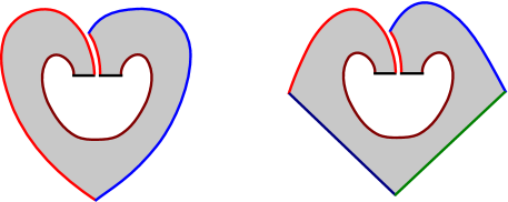
Figure 9. The domains $D_{1}$ (a) and $D_{3}$ (b).

Domains with a boundary cut

Let

$$D_{1}=R_{7}+R_{8}+R_{19}+\dots+R_{30}+R_{36}+R_{37}+R_{49}+R_{50}+R_{51}+R_{52},$$

For any $i\in\{38,39,40,43,44,45\}$ $D_{1}$ represents a class in $\pi_{2}(x_{15}x_{i},x_{22}x_{i})$ and has index $1$ with respect to the sequence $(-\rho_{2},-\rho_{3})$. (If $i\in\{47,\dots,52\}$, the index is $3$ rather than $1$.) To obtain a holomorphic representative of $D_{1}$ compatible with $(-\rho_{2},-\rho_{3})$, we cut along $\alpha_{1}^{L}$ all the way to the boundary, as shown in Figure 9. Thus, we parametrize $D_{1}$ as a bigon with two separate boundary punctures rather than as an annulus with a single puncture (which is prohibited by Proposition 2.1). It is then straightforward to see that $D_{1}$ supports a unique holomorphic representative and thus provides a differential $x_{15}x_{i}\xrightarrow{\rho_{23}\otimes\mathbf{1}}x_{22}x_{i}$ for each $i$ as above. Likewise, for each $j\in\{36,37,41,42,46\}$, the domain

$$D_{2}=R_{4}+R_{11}+R_{17}+R_{20}+R_{24}+R_{25}+R_{29}+R_{32}+R_{35}+R_{39}+R_{43}+R_{47}+R_{50},$$

representing a class in $\pi_{2}(x_{35}x_{j},x_{1}x_{j})$, contributes a differential $x_{35}x_{j}\xrightarrow{\mathbf{1}\otimes\sigma_{12}}x_{1}x_{j}$. In fact, $D_{1}$ and $D_{2}$ are the only domains of this form (so they account for $11$ of the $1,013$ total classes).

Similarly, the domains

$$D_{3} =R_{7}+R_{8}+R_{31}+R_{36}+R_{37}+R_{48}$$

$$D_{4} =D_{2}+R_{4}+R_{5}+R_{10}+R_{11}+R_{17}+R_{18}+R_{24}+R_{25}+R_{29}+R_{30}+R_{32}$$

$$\qquad+R_{36}+R_{37}+R_{38}+R_{39}+R_{47}+R_{49}+R_{50},$$

respectively represent index-$1$ classes in $\pi_{2}(x_{22}x_{45},x_{23}x_{46})$, and $\pi_{2}(x_{35}x_{46},x_{2}x_{48})$. The source curve for $D_{3}$ or $D_{4}$ is a quadrilateral, with two boundary punctures on one $\alpha$ edge mapping to $-\rho_{2}$ and $-\rho_{3}$ and (for $D_{4}$) a boundary puncture on the other $\alpha$ edge mapping to $\sigma_{1}$. It is easy to see that these classes all support holomorphic representatives. Thus, we have differentials $x_{15}x_{i}\xrightarrow{\rho_{23}\otimes\mathbf{1}}x_{22}x_{i}$, $x_{22}x_{45}\xrightarrow{\rho_{23}\otimes\mathbf{1}}x_{23}x_{46}$, and $x_{35}x_{46}\xrightarrow{\rho_{23}\otimes\sigma_{1}}x_{2}x_{48}$. We find $41$ domains of this form.

(a) at 18 145 (b) at 203 145 $x_{23}$ at 80 150 $x_{30}$ at 80 17 $\alpha_{2}^{R}$ at 45 128 $\beta_{1}$ at 115 128 $\alpha_{2}^{L}$ at 65 33 $\alpha_{1}^{L}$ at 81 101 $\rho_{23}$ at 45 49 $x_{23}$ at 192 88 $x_{15}$ at 274 15 $x_{46}$ at 358 88 $x_{52}$ at 274 142 $\alpha_{2}^{R}$ at 217 128 $\beta_{2}$ at 335 128 $\beta_{1}$ at 224 58 $\alpha_{1}^{L}$ at 326 58 $\alpha_{2}^{L}$ at 246 122 $\rho_{23}$ at 246 96

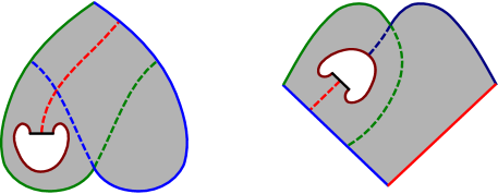
Figure 10. The domains $D_{5}$ (a) and $D_{6}$ (b).

Domains without a boundary cut

Let

$$D_{5} =R_{7}+R_{8}+R_{36}+R_{37}+R_{48}+R_{49}+R_{50}+R_{51}+R_{52}$$

$$D_{6} =R_{7}+R_{8}+R_{19}+R_{20}+R_{21}+R_{22}+R_{23}+R_{24}+R_{36}+R_{37},$$

illustrated in Figure 10. $D_{5}$ represents a class in $\pi_{2}(x_{30}x_{j},x_{23}x_{j})$ for each $j\in\{37,41,42,46\}$, and $D_{6}$ represents a class in $\pi_{2}(x_{15}x_{52},x_{23}x_{46})$. We cannot cut these domains along $\alpha_{1}^{L}$ as we did with $D_{3}$ and $D_{4}$, since in each case, as we travel along $\alpha_{1}^{L}$ from the intersection point of $\rho_{2}\cap\rho_{3}$, we reach the boundary of $D_{5}$ (resp. $D_{6}$) before reaching $x_{j}$ (resp. $x_{46}$). Thus, $D_{5}$ and $D_{6}$ cannot admit holomorphic representatives. We find $106$ domains like $D_{5}$ and $62$ domains like $D_{6}$. (Some of these domains have additional $\sigma_{2}$ or $\sigma_{3}$ punctures on their boundaries, but these do not affect the argument above.)

We also find domains such as

$$D_{7}=R_{7}+R_{8}+R_{14}+R_{36}+R_{37}+R_{42}$$

which are the disjoint union of an annulus, one of whose boundary component equals $\alpha_{2}^{L}\cup\rho_{2}\cup\rho_{3}$, and a bigon. Since the $\alpha_{2}^{L}\cup\rho_{2}\cup\rho_{3}$ boundary component of the annulus does not contain a point of either the source or the target generator, there is no way to find a source surface representing $D_{7}$. We find $37$ domains of this form.

Indecomposable annuli

Consider the domains

$$D_{8} =R_{8}+R_{9}+R_{10}+R_{18}+R_{31}+R_{38}+R_{48}\in\pi_{2}(x_{4}x_{38},x_{6}x_{52})$$

$$D_{9} =R_{2}+R_{6}+R_{7}+R_{8}+R_{14}+R_{36}+R_{37}+R_{42}\in\pi_{2}(x_{21}x_{36},x_{23}x_{37})$$

shown in Figure 11. Each of these domains is topologically an annulus with three convex corners and one concave corner and cannot be decomposed as the composition of an index-0 annulus and a bigon (in contrast to another family of annuli considered below). As illustrated in Figure 11, we call the boundary component containing the convex corner the outer boundary and the other component the inner boundary. There are a total of eight domains with the geometry of $D_{8}$ and fifteen with the geometry of $D_{9}$.

(a) at 18 158 (b) at 176 158 (c) at 348 158 $x_{4}$ at 80 155 $x_{6}$ at 80 22 $x_{38}$ at 80 72 $x_{52}$ at 80 92 $\alpha_{1}^{L}$ at 43 128 $\beta_{1}$ at 117 128 $\alpha_{2}^{R}$ at 63 81 $\beta_{2}$ at 99 81 $x_{6}$ at 237 147 $x_{37}$ at 237 13 $x_{23}$ at 218 87 $x_{21}$ at 218 108 $\alpha_{2}^{R}$ at 235 96 $\beta_{2}$ at 307 128 $\beta_{1}$ at 200 96 $\alpha_{1}^{L}$ at 214 29 $\alpha_{2}^{L}$ at 169 128 $\rho_{123}$ at 180 50 $x_{4}$ at 395 155 $x_{22}$ at 395 11 $x_{j}$ at 399 83 $\alpha_{1}^{L}$ at 356 128 $\beta_{1}$ at 433 128 $\alpha_{2}^{R}$ at 423 92 $\beta_{2}$ at 385 94

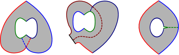
Figure 11. The indecomposable annuli $D_{8}$ (a), $D_{9}$ (b), and $D_{10}$ (c).

Lemma 3.3.

For any complex structure on $\Sigma$, the moduli spaces $\mathcal{M}(D_{8})$ and $\mathcal{M}(D_{9})$ each contain an odd number of points. Thus, $D_{8}$ and $D_{9}$ always count for the differential.

Proof.

Given a choice of complex structure on $\Sigma$, each domain admits a one-dimensional family of conformal structures, depending on the value of a cut parameter $c\in\mathbb{R}$, where $c<0$ corresponds to cutting along the $\alpha$ curve and $c>0$ corresponds to cutting along the $\beta$ curve. For each value of the cut parameter $c$, let $\theta_{0}(c)$ (resp. $\theta_{1}(c)$) denote the ratio of the conformal length of the $\alpha$ arc of the outer (resp. inner) boundary to the conformal length of the $\beta$ arc of the outer (resp. inner) boundary. A given conformal structure admits a holomorphic involution if and only if $\theta_{0}(c)=\theta_{1}(c)$, so the number of points in the moduli space of each domain (modulo 2) equals the number of zeros of the function $f(c)=\theta_{0}(c)-\theta_{1}(c)$, which for generic choices of complex structure on $\Sigma$ can be assumed to be transverse to $0$. This number is determined by the limiting behavior of $f(c)$, as follows.

For $D_{8}$, the cut in the $\alpha$ direction approaches the $\beta$ arc of the inner boundary and the cut in the $\beta$ direction approaches the $\alpha$ arc of the inner boundary. Thus, in the limit as we cut in the $\alpha$ direction, $\theta_{0}(c)$ becomes arbitrarily large and $\theta_{1}(c)$ approaches $0$, so $\lim_{c\to-\infty}f(c)=\infty$. Similarly, as we cut in the $\beta$ direction, $\theta_{0}(c)$ approaches $0$ and $\theta_{1}(c)$ becomes arbitrarily large, so $\lim_{c\to\infty}f(c)=-\infty$. By transversality and the intermediate value theorem, $f(c)$ has an odd number of zeros.

For $D_{9}$, there is a Reeb chord marked $\rho_{123}$ on the outer boundary. The cut in the $\beta$ direction approaches the $\alpha$ arc of the inner boundary, while the cut in the $\alpha$ direction approaches this boundary puncture. Thus, as we cut in the $\alpha$ direction, $\theta_{0}(c)$ becomes arbitrarily large, while $\theta_{1}(c)$ approaches a finite value. Thus, $\lim_{c\to-\infty}f(c)=\infty$, while $\lim_{c\to\infty}f(c)=-\infty$ just as with $D_{8}$. ∎

Similarly, the annular domain

$$D_{10}=\sum_{i=8}^{24}R_{i}$$

represents an index-1 class in $\pi_{2}(x_{4}x_{j},x_{22}x_{j})$ for any of the twelve points $x_{j}\in(\alpha_{1}^{R}\cup\alpha_{2}^{R})\cap\beta_{2}$. This domain similarly admits a 1-dimensional family of conformal structures given by a cut parameter by $c\in(0,\infty)$. As we increase the cut parameter, the ratio of the length of the $\alpha$ segment of the boundary component containing $x_{j}$ to the $\beta$ segment of the same tends from $0$ to infinity, while the same ratio on the opposite boundary component tends from a finite value to $0$. Thus, $D_{10}$ counts for the differential for each choice of $x_{j}$.

Decomposable annuli

We next consider domains whose moduli spaces may depend nontrivially on the choice of complex structure. As a preliminary, let $\eta\subset\Sigma$ be a simple closed curve passing through the regions $R_{1}$, and $R_{4},\dots,R_{12}$. For a given complex structure $J$ on $\Sigma$ and $T\in[0,\infty)$, let $J_{T}$ denote the complex structure obtained by “stretching the neck” along $\eta$ by inserting an annulus of width $T$.

Consider the following domains:

(3.1) $$A_{1} =R_{7}+R_{8}+R_{48}+R_{49}+R_{30}+R_{31}$$

$$A_{2} =A_{1}+R_{24}+R_{25}+R_{47}+R_{50}+R_{29}+R_{32}$$

$$A_{3} =A_{2}+R_{23}+R_{26}+R_{46}+R_{51}+R_{28}+R_{33}$$

$$A_{4} =A_{1}+R_{6}+R_{9}$$

$$A_{5} =A_{2}+R_{6}+R_{9}$$

$$A_{6} =A_{3}+R_{6}+R_{9}$$

Each of these domains is an index-$0$ annulus, with one boundary component consisting of a segment of $\beta_{1}$ and a segment of $\alpha_{1}^{L}$ or $\alpha_{2}^{L}$ and the other consisting of a segment of $\beta_{2}$ and a segment of $\alpha_{1}^{R}$ or $\alpha_{2}^{R}$. We call these the two boundary components the outer boundary and inner boundary, respectively. A choice of complex structure $J$ on $\Sigma$ completely determines a conformal structure on each $A_{i}$. Let $\Theta_{0}^{i}(J)$ (resp. $(\Theta_{1}^{i}(J))$) denote the ratio of the conformal length of the $\alpha$ segment of the inner (resp. outer) boundary of $A_{i}$ to the conformal length of the $\beta$ segment of the inner (resp. outer) boundary. We say that $J$ is sufficiently stretched if $\Theta_{0}^{i}(J)>\Theta_{1}^{i}(J)$ for each $i=1,\dots,6$.

Lemma 3.4.

For any complex structure $J$ on $\Sigma$ there exists a number $T_{0}=T_{0}(J)$ such that for any $T>T_{0}$, the complex structure $J_{T}$ is sufficiently stretched.

Proof.

For each $i$, the only intersections of the curve $\eta$ with the boundary of $A_{i}$ are on the $\alpha$ segment of the outer boundary, so stretching the neck along $\eta$ increases the conformal length of that segment relative to the $\beta$ segment of the outer boundary. Therefore, for large values of $T$, $\Theta_{0}^{i}(J_{T})$ can be made arbitrarily large, while $\Theta_{1}^{i}(J_{T})$ approaches some finite value. ∎

Consider the index-$1$ annuli

(3.2) $$D_{11} =A_{1}+R_{36}\in\pi_{2}(x_{4}x_{45},x_{5}x_{47})$$

$$D_{12} =A_{1}+R_{37}\in\pi_{2}(x_{3}x_{45},x_{4}x_{47})$$

$$D_{13} =A_{1}+R_{25}+R_{26}+R_{27}+R_{28}+R_{29}+R_{50}+R_{51}+R_{52}$$

$$\qquad\qquad\qquad\in\pi_{2}(x_{3}x_{45},x_{5}x_{52})$$

$$D_{14} =A_{1}+R_{2}+R_{14}+R_{36}+R_{37}+R_{42}\in\pi_{2}(x_{3}x_{45},x_{2}x_{47})$$

$$D_{15} =A_{1}+R_{2}+R_{6}+R_{9}+R_{14}+R_{42}\in\pi_{2}(x_{3}x_{45},x_{6}x_{47})$$

$$D_{16} =A_{1}+R_{20}+R_{24}+R_{25}+R_{29}+R_{32}+R_{35}+R_{43}+R_{47}+R_{50}$$

$$\qquad\qquad\qquad\in\pi_{2}(x_{3}x_{44},x_{5}x_{47}),$$

some of which are shown in Figure 12. Each of these annuli can be written as a sum of an index-0 annulus and an adjacent bigon, so we call these domains decomposable. It is easy to find eighteen other domains of this form, where we take $A_{2},\dots,A_{6}$ in place of $A_{1}$ in (3.2) as applicable. Note that $D_{15}$ and $D_{16}$ can each be decomposed into the sum of an index-0 annulus and an adjacent bigon in a second way as well:

(3.3) $$D_{15} =A_{4}+R_{2}+R_{14}+R_{42}$$

$$D_{16} =A_{2}+R_{20}+R_{35}+R_{43},$$

We therefore call these domains doubly decomposable.

(a) at 18 158 (b) at 169 158 (c) at 318 158 $x_{4}$ at 80 143 $x_{5}$ at 80 11 $x_{45}$ at 80 56 $x_{47}$ at 80 95 $\rho_{2}$ at 49 156 $\alpha_{1}^{L}$ at 66 150 $\alpha_{2}^{L}$ at 32 50 $\beta_{1}$ at 126 150 $\alpha_{2}^{R}$ at 63 83 $\beta_{2}$ at 98 83 $x_{3}$ at 231 143 $x_{2}$ at 231 11 $x_{45}$ at 199 91 $x_{47}$ at 199 135 $\alpha_{2}^{R}$ at 191 113 $\beta_{2}$ at 210 113 $\beta_{1}$ at 278 50 $\alpha_{1}^{L}$ at 205 27 $\alpha_{2}^{L}$ at 162 93 $\rho_{123}$ at 175 47 $x_{3}$ at 380 143 $x_{6}$ at 380 11 $x_{45}$ at 409 76 $x_{47}$ at 409 126 $\rho_{1}$ at 351 156 $\alpha_{2}^{L}$ at 366 150 $\alpha_{1}^{L}$ at 333 50 $\beta_{1}$ at 426 50 $\alpha_{2}^{R}$ at 398 100 $\beta_{2}$ at 420 100

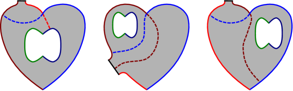
Figure 12. The decomposable annuli $D_{11}$ (a), $D_{14}$ (b), and $D_{15}$ (c).

Lemma 3.5.

If $J$ is sufficiently stretched, the moduli spaces of all of the decomposable annuli each contain an even number of points. Thus, these domains do not count for the differential.

Proof.

We begin with $D_{11}$. Just as with the indecomposable annuli discussed above, there is a $1$-dimensional family of conformal structures on $D_{11}$ given by a cut parameter at $x_{4}$. As we cut along $\alpha_{1}^{L}$, the cut approaches the $\beta$ arc of the inner boundary, $\theta_{0}(c)$ becomes arbitrarily large while $\theta_{1}(c)$ approaches $0$, so $\lim_{c\to-\infty}f(c)=\infty$. On the other hand, cutting along $\beta_{1}$ degenerates $D_{11}$ into $A_{1}$ and a bigon (with a Reeb chord). By Gromov compactness, in the limit as $c\to\infty$, the ratios $\theta_{0}(c)$ and $\theta_{1}(c)$ approach the corresponding parameters for $A_{1}$, namely $\Theta_{0}^{1}(J_{T})$ and $\Theta_{1}^{1}(J_{T})$. By Lemma 3.4, if we choose $T$ large enough that $\Theta_{0}^{1}(J_{T})>\Theta_{1}^{1}(J_{T})$, we see that $\lim_{c\to\infty}f(c)>0$, so $f(c)$ has an even number of zeroes, as required.

The arguments for $D_{12}$, $D_{13}$, and $D_{14}$ are very similar. The one modification for $D_{14}$ is that as we cut along $\alpha_{2}^{L}$ at $x_{3}$ out to the boundary puncture, $\theta_{1}(c)$ approaches a finite value that is not necessarily zero, just as we saw with $D_{8}$ above. However, $\theta_{0}(c)$ still approaches $\infty$, so the remainder of the argument carries through unchanged.

For $D_{15}$, cutting along $\alpha_{2}^{L}$ at $x_{3}$ decomposes the domain as in (3.2), while cutting along $\beta_{1}$ decomposes it as in (3.3). Therefore, $\lim_{c\to-\infty}f(c)=\Theta_{0}^{1}(J_{T})-\Theta_{1}^{1}(J_{T})$ and $\lim_{c\to\infty}f(c)=\Theta_{0}^{4}(J_{T})-\Theta_{1}^{4}(J_{T})$. By Lemma 3.4, we may choose $T$ large enough such that both of these limits are positive numbers, which implies that $f(c)$ has an even number of zeroes. The same analysis goes through for $D_{16}$. ∎

Genus-1 classes

Having analyzed all the classes represented by planar surfaces, we now turn to classes that are represented by surfaces of genus $1$. It is difficult to determine whether these classes support holomorphic representatives using direct conformal geometry arguments as above. Instead, we will look at how these domains arise in the broken flowlines that are the ends of 1-dimensional moduli spaces — specifically, the fact the relation $\partial^{2}=0$ and its more complicated $\mathcal{A}_{\infty}$ analogues — to deduce the behavior of these domains indirectly. We shall see that knowledge of the planar classes completely determines which of the genus-1 classes count for the differential.

(a) at 10 150 (b) at 134 150 $x_{3}$ at 13 14 $x_{23}$ at 13 135 $x_{36}$ at 89 57 $x_{52}$ at 89 92 $\alpha_{2}^{L}$ at 104 35 $\beta_{1}$ at 11 76 $\alpha_{2}^{R}$ at 104 114 $\beta_{2}$ at 88 76 $x_{3}$ at 135 14 $x_{16}$ at 135 135 $x_{36}$ at 211 57 $x_{45}$ at 211 92 $\alpha_{2}^{L}$ at 226 35 $\beta_{1}$ at 133 76 $\alpha_{2}^{R}$ at 244 114 $\beta_{2}$ at 210 76

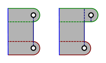
Figure 13. The embedded genus-1 domains $D_{17}$ (a) and $D_{18}$ (b).