The life-cycle of drift-wave turbulence driven by small scale instability

Abstract

We demonstrate theoretically and numerically the zonal-flow/drift-wave feedback mechanism for the LH transition in an idealised model of plasma turbulence driven by a small scale instability. Zonal flows are generated by a secondary modulational instability of the modes which are directly driven by the primary instability. The zonal flows then suppress the small scales thereby arresting the energy injection into the system, a process which can be described using nonlocal wave turbulence theory. Finally, the arrest of the energy input results in saturation of the zonal flows at a level which can be estimated from the theory and the system reaches stationarity without damping of the large scales.

Designing a device capable of controlled, self-sustained nuclear fusion is one of the principal technological challenges of the 21st century. Attention is now heavily focused on the construction of the International Thermonuclear Test Reactor (ITER) which aims to demonstrate the feasibility of controlled fusion for the first time. Of the myriad of engineering challenges posed by ITER, one of the most critical, the problem of magnetic plasma confinement, relates intimately to foundational issues in turbulence theory, the topic of this Letter. One difficulty of magnetic plasma confinement is due to instabilities (such as the ion temperature gradient, drift-dissipative and electron temperature gradient instabilities). These generate waves which interact to produce wave turbulence thereby greatly enhancing transport. Heat and plasma then diffuse more quickly from the hot, dense core to the periphery resulting in a loss of confinement. Common features of these instabilities are that they are small scale, typically of the order of the ion gyro-radius or below, and principally generate meridional waves (with wave crests along the minor radius of the torus).

Significant progress in the confinement problem came with the experimental discovery Wagner et al. (1982) that, under the right conditions, the turbulent transport coefficient suddenly drops. This effect, called the Low-to-High (LH) confinement transition, can be exploited to design more efficient confinement. Although traces of the LH transition were replicated in numerical simulations Numata et al. (2007), including full gyro-kinetic calculations Villard et al. (2004), the underlying mechanism was initially poorly understood since realistic numerical simulations of tokamaks are universally incapable of resolving the full range of scales involved. It is now generally accepted Diamond et al. (2005) that the LH transition is triggered by the self-organisation of coherent zonal flows (ZF’s) in the poloidal direction which act as transport barriers since they act to shear away turbulent fluctuations which try to cross them. Current research is heavily focused on understanding and parameterising these ZF’s and their interaction with the drift wave turbulence at the experimental, numerical and theoretical levels.

In this Letter we present a simple theoretical model of the confinement mechanism described above. Our model uses the Charney-Hasegawa-Mima (CHM) equation Hasegawa and Mima (1977), the simplest single-fluid description of a strongly magnetised plasma. This equation is rarely used in modern plasma research because drastic simplifications are required to obtain it from the true dynamical equations. On the other hand, simple models often repay in terms of analytical tractability and conceptual clarity what they lose in terms of direct applicability. This is certainly the case here. Our model gives a semi-analytical description of the full life-cycle of turbulence generated by a small-scale primary instability. Before presenting details, we outline the main results. Meridional waves - drift waves in the case of the CHM model - are generated by a primary instability at the scale of the ion gyro-radius. The subsequent evolution has three main stages. In stage 1, waves grow until they generate seeds of a ZF via a secondary modulational instability Manin and Nazarenko (1994); Onishchenko et al. (2004); Connaughton et al. (2010a). The ZF is large-scale compared to the waves. In stage 2, the ZF’s grows by direct interaction with the small scales rather than by a Kraichnan-style inverse cascade which would involve local transfer of energy between scales. This is because the nonlocal interaction in drift wave turbulence is intrinsic, i.e. it typically develops in time even for broadband initial spectra. However, the fact that the primary instability produces a relatively narrow initial drift-wave spectrum helps nonlocality. Due to nonlocality, the kinetic energy of the small scales is not conserved as it would be in a local cascade. In fact, the growing ZF removes energy from the turbulence since the combined energy of large and small scales is conserved. The wave turbulence which gave birth to the ZF in stage 1 is thus suppressed by its growth. In stage 3, this negative feedback reaches a steady state in which suppression of turbulence by the large-scale ZF exactly balances its generation by the small scale instability. We note that Eq. (1) also has a geophysical interpretation which we do not discuss (see references in Connaughton et al. (2010a)).

The CHM model does not contain small scale instabilities of the kind mentioned above. In what follows, we model these instabilities with a multiplicative linear forcing term applied to selected wavenumbers. We solve the following equation on a plane with the $x$-axis along the plasma density gradient $\nabla n_{0}$ and the $y$-axis transverse to this:

$$\left(\partial_{t}-{\mathcal{L}}\right)\left(\rho^{2}\Delta\psi-\psi\right)+v_{*}\,\partial_{y}\psi-\rho^{2}J[\psi,\Delta\psi]=0.$$ (1)

Here $\psi(x,y,t)$ is the streamfunction, $\Delta$ is the 2D Laplacian, $J[\psi,\Delta\psi]=\partial_{x}\psi\partial_{y}\Delta\psi-\partial_{y}\psi\partial_{x}\Delta\psi$ and ${\mathcal{L}}$ is a linear operator having Fourier-space representation ${\mathcal{L}}_{{\bf k}}=\gamma_{\bf k}-\nu_{m}k^{2m}$ with $\gamma_{\bf k}>0$ modeling the instability and $\nu_{m}$ a hyperviscosity coefficient. Here, $\rho$ is the ion Larmor radius at the electron temperature, $v_{*}=\omega_{B}\rho^{2}/L_{n}$ is the drift velocity, $\omega_{B}$ is the ion gyro-frequency and $L_{n}=n_{0}/|\nabla n_{0}|$ is the density profile length-scale. $\rho$ and $v_{*}$ are both taken to be constant. For the instability forcing, $\gamma_{\bf k}$, we seek the simplest form which retains the key features of the relevant plasma instabilities mentioned above, namely that they act at small scales and primarily generate meridional waves. For these purposes it suffices to take $\gamma_{{\bf k}}=\gamma\,\delta_{{\bf k},{\bf k}_{i}}$, with ${\bf k}_{i}=(0,\rho^{-1})$ and $\gamma>0$, which forces a single meriodinal mode at the scale of the gyro-radius. In principle, a more realistic form for $\gamma_{\bf k}$ can be obtained by considering the linear dynamics of a higher level model which does contain an intrinsic instability such as the Hasegawa-Wakatani (HW) model in the case of the drift-dissipative instability Numata et al. (2007). The dimensionless parameter, $\chi=\frac{\gamma\rho}{v_{*}}$, is a measure of nonlinearity of the system assuming that the linear instability saturates at a level determined by the amplitude of the nonlinear term in Eq.(1). Eq. (1) has exact plane wave solutions $\psi=\exp(-i(\omega_{\bf k}t-{\bf k}\cdot{\bf x})+\gamma_{\bf k}t-\nu_{m}k^{2m}t)$ with dispersion relation, $\omega_{\bf k}=-v_{*}k_{y}/(1+\rho^{2}k^{2})$.

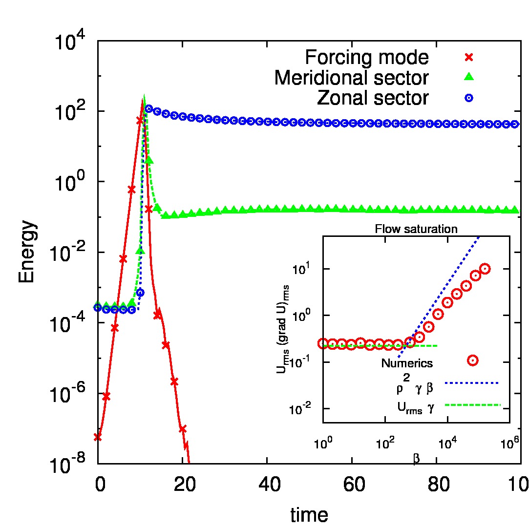
Figure 1: (color online) Energy contained in the forced mode (crosses), the zonal sector (circles) and meridional sector (triangles) as functions of time for $\chi=3.75\times 10^{-4}$. The inset shows the saturation level of the ZF as a function of $\beta$.

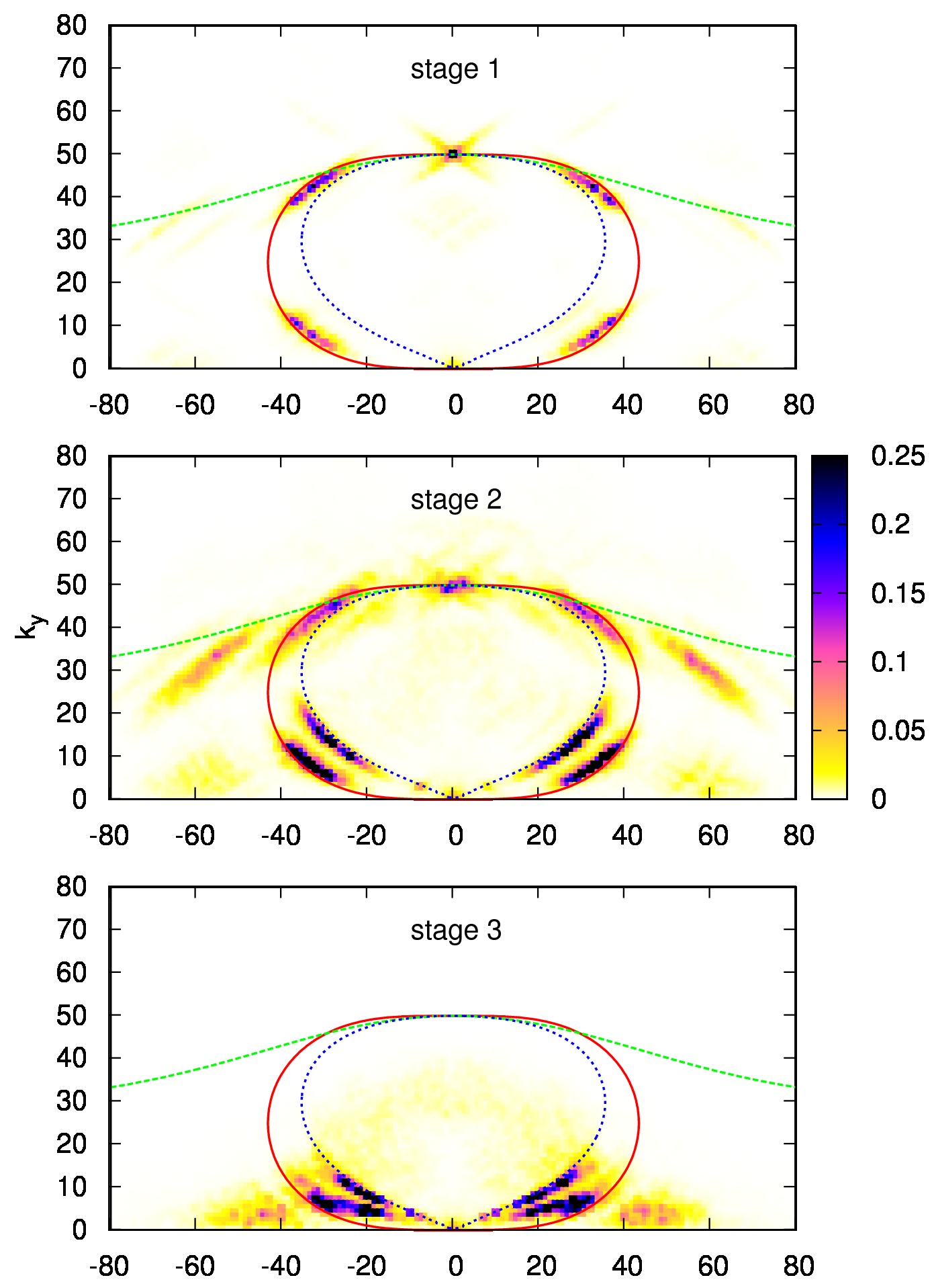
Figure 2: (color online) Snapshots of the 2D energy spectrum at times $11.0$, $11.5$ and $20$ for the case $\chi=3.74\times 10^{-4}$

Without instability or dissipation (${\mathcal{L}}\equiv 0$), Eq. (1) has two invariants: $E=\frac{1}{2}\int[\rho^{-2}\psi^{2}+(\nabla\psi)^{2}]\,d{\bf x}$ and $\Omega=\frac{1}{2}\int[\rho^{-2}(\nabla\psi)^{2}+(\nabla^{2}\psi)^{2}]\,d{\bf x}$. These are closly related to the energy and enstrophy in the 2D Euler equations. 2D Euler turbulence exhibits an inverse cascade of energy from small scales to large. Likewise, CHM turbulence transfers energy to large scales. In the weakly nonlinear limit, however, CHM turbulence differs from 2D Euler turbulence in some important respects. Firstly, in this limit, the energy transfer turns out to be nonlocal in scale Balk et al. (1990) meaning that it is dominated by interactions between the smallest and largest scales. Secondly, there is an additional statistical invariant, the zonostrophy Balk et al. (1991), which renders the transfer anisotropic Balk et al. (1991); Nazarenko and Quinn (2009). The theory of nonlocal drift wave turbulence was first worked out in Balk et al. (1990); Nazarenko, S.V. (1991) and a detailed summary can be found in Connaughton et al. (2010b). In this Letter, we will present a self-consistent but qualitative physical argument to arrive at the same results.

Consider a drift wavepacket with wavenumber ${\mathbf{k}}$ moving on a background consisting of a large-scale ZF with typical wavenumber ${\mathbf{p}}$. The ZF need not be perfect and can have finite $p_{x}$, but we insist that it is large scale: $p\ll k$ and $p\ll 1/\rho$ so that a the WKB approximation is appropriate Dyachenko et al. (1992). The ZF is stationary in a frame moving in the $y$-direction with the drift velocity $v_{*}$ Connaughton et al. (2010b). As a consequence of the WKB approximation, the wave packet frequency must be conserved in this frame:

$$v_{*}k_{y}+\omega_{\mathbf{k}}=\frac{v_{*}k_{y}\rho^{2}k^{2}}{1+\rho^{2}k^{2}}=k^{2}\,\omega_{\mathbf{k}}=v=\mbox{const}.$$ (2)

Hence, as ${\mathbf{k}}$ changes due to distortion of the wavepacket by the ZF, it is restricted to remain on the 1D curve in the 2D ${\mathbf{k}}$-space given by (2), hereafter called a $v$-curve. A typical $v$-curve is indicated by the green (dashed) line in Fig. 2. According to WKB theory, it is waveaction of the small scales, $n_{\mathbf{k}}=e_{\mathbf{k}}/\omega_{\mathbf{k}}$, which is conserved rather than the energy, $e_{\mathbf{k}}$. On each $v$-curve, $n_{\mathbf{k}}\sim k^{2}e_{\mathbf{k}}$ from Eq. (2). Since $k^{2}$ increases as a wavepacket moves along a $v$-curve from the source (at the $k_{y}$-axis) to the sink (at high $k$’s), $e_{\mathbf{k}}$ must decrease to keep $n_{\mathbf{k}}$ constant. The energy thus lost is transferred to the ZF.

There are two qualitatively different regimes corresponding to weak and strong ZFs. The weak regime occurs when drift wave packets live long enough to cross many ZF oscillations, experiencing multiple random distortions and executing a random walk in $\bf k$-space along the $v$-curves. It can be described by a diffusion equation:

$$\frac{\partial n_{\mathbf{k}}}{\partial t}=\partial_{v}\left(D_{\mathbf{k}}\partial_{v}n_{\mathbf{k}}\right)+\gamma_{\mathbf{k}}n_{\mathbf{k}}-\nu_{m}k^{2m}n_{\mathbf{k}},$$ (3)

where $\partial_{v}$ is the derivative along the $v$-curve. A detailed quantitative derivation of Eq. (3) is presented in Connaughton et al. (2010b). The diffusion coefficient, $D_{\mathbf{k}}$, is proportional to the intensity of the large-scale ZF, and can be estimated as $D_{\mathbf{k}}\sim(\dot{k}_{x})^{2}\tau,$ where $\dot{k}_{x}\sim-k_{y}S$ is the rate of change of $k_{x}$ due to the ZF shear $S=\partial_{x}U\sim pU$, and $\tau$ is the correlation time $\tau={1/(p|{\dot{x}}|)}={1/(p|{\partial_{k_{x}}\omega_{k}}|)}\sim{1/(pv_{*})}.$ In these estimates we took into account that the essential dynamics happens at the scales $k_{x}\sim k_{y}\sim 1/\rho$. Thus

$$D_{\mathbf{k}}\sim\frac{S^{2}}{\rho^{2}v_{*}p}\sim\frac{SU}{\rho^{2}v_{*}}.$$ (4)

For fixed $D_{\mathbf{k}}$, Eq. (3) indicates that $n_{\mathbf{k}}$ evolves independently on each $v$-curve and is controlled by the maximum value of $\lambda_{\mathbf{k}}=\gamma_{\mathbf{k}}-\nu_{m}k^{2m}$ on the curve. If $\lambda_{\mathbf{k}}$ is positive, $n_{\mathbf{k}}$ will initially grow exponentially. Correspondingly, if $\lambda_{\mathbf{k}}$ is negative, $n_{\mathbf{k}}$ will be exponentially damped. Large positive $\lambda_{\mathbf{k}}$ are obtained on curves passing close to the maximum of $\gamma_{k}$. In our case this is the forcing mode, ${\mathbf{k}}=(0,k_{i})$. Negative values are found away from this maximum, where dissipation dominates. The growth of $n_{\mathbf{k}}$ on a $v$-curve with positive $\lambda_{\mathbf{k}}$ cannot, however, continue indefinitely. Diffusion along a curve transfers energy to large scales. This in turn increases $D_{\mathbf{k}}$ so that the growth due to positive $\lambda_{\mathbf{k}}$ can begin to be tempered by increasingly rapid diffusion of wavepackets from the instability region to the dissipation region. The region of growing $n_{\mathbf{k}}$ shrinks until a steady state is reached (stage 3). Those $v$-curves which originally had positive growth reduce their growth rates to zero and the spectrum on them dies out. The large-scale ZF in turn saturates at a finite intensity determined by balancing the forcing and the diffusion terms on the right hand side of Eq. (3), giving $D_{\mathbf{k}}\rho^{2}\sim\gamma_{\mathrm{max}}.$ Eq. (4) gives the saturation criterion:

$$U_{\mathrm{rms}}S_{\mathrm{rms}}\sim v_{*}\gamma_{\mathrm{max}}.$$ (5)

where rms denotes root-mean square. Counterintuitively, the saturation velocity increases with $v_{*}$ as the flow becomes more linear. Eq. (5) fails for large $\chi$ when turbulence is strong and the $v_{*}$-term in Eq. (1)can be neglected. In the strong turbulence regime, a wavepacket cannot cross even a single ZF oscillation since rapid distortion by the zonal shear brings its wavenumber to the dissipation scale. This gives the saturation criterion

$$S_{\mathrm{rms}}\sim\gamma_{\mathrm{max}}.$$ (6)

Comparing Eqs. (5) and (6), the crossover between the two regimes occurs when $\gamma_{\mathrm{max}}\sim v_{*}p$ or when $U_{\mathrm{rms}}\sim v_{*}$. The estimate (6), previously put forward in Kingsbury and Waltz (1994), is valid only for strong ZF’s with $U_{\mathrm{rms}}\gtrsim v_{*}$.

We performed numerical simulations using a standard pseudo-spectral code at a resolution of $256\times 256$ with $m=8$, $\nu_{m}=1.0\times 10^{-29}$, $\rho=0.02$ and $\gamma=1.2$. The initial condition was spatial white noise of very low amplitude. Fig. 1 summarizes results obtained with $\beta=1.6\times 10^{5}$ giving $\chi=3.75\times 10^{-4}$. We divided ${\bf k}$-space into a zonal sector, $\left|k_{x}\right|>\left|k_{y}\right|$, and a meridional sector, $\left|k_{x}\right|\leq\left|k_{y}\right|$ (excluding the forced mode). Fig. 1 shows the energy of each sector and of the forced mode as functions of time. Initially, the forced mode grows exponentially, and the zonal and meridional energies remain at a level set by the initial noise. This is followed by a sharp growth of the the zonal and the off-zonal energies once the amplitude of the forced mode gets high enough to facilitate nonlinear mode coupling (stage 1). Next, the meridional modes, including the forced mode itself, are suppressed while the zonal modes retain their energy (stage 2). Finally a steady state is reached (stage 3) in which the instability forcing is switched off and the majority of the energy is zonal.

Fig. 2 shows the time evolution of the 2D energy spectrum in $\bf k$-space normalized by the maximum. The forced mode initially dominates but such waves are modulationally unstable Manin and Nazarenko (1994); Onishchenko et al. (2004); Connaughton et al. (2010a). The first indication of the nonlinear evolution seen in stage 1 is therefore the growth from the background noise of those modes whose modulational instability growth rate is greatest. In the limit of weak nonlinearity, the modulationally unstable modes concentrate on the resonant curve passing through the forcing mode, $\omega({\mathbf{k}})=\omega({\mathbf{k}}_{1})+\omega({\mathbf{k}}_{2})$ with ${\mathbf{k}}={\mathbf{k}}_{1}+{\mathbf{k}}_{2}$ for ${\mathbf{k}_{3}}=(k_{i},0)$ Connaughton et al. (2010a). The maximally unstable perturbations of a meridional wave have a significant zonal component (see Fig. 2 of Connaughton et al. (2010a)). These are visible, along with the resonant curve, in the left panel of Fig. 2. They are the seeds of the ZF’s responsible for the LH transition. The very rapid decrease in meridional turbulent energy observed in Fig. 1 at stage 2 is related with the ZF-induced diffusion along the $v$-curves with a diffusion coefficient growing as the ZF is becoming stronger. This diffusion process is clearly visible in the middle frame of Fig. 2. Deviations from the theoretical $v$-curve can be attributed to absence of a large scale separation between the forcing and the zonal modes assumed in the derivation of Eq. (3). We remark that if there is a nonlocal interaction with small-scale ZF’s then diffusion proceeds along different curves, the level sets of zonostrophy Nazarenko, S.V. (1991); Connaughton et al. (2010b). One such curve, passing through the forced mode is shown in Fig. 2 by the blue dashed line. A secondary ZF branch emerges on this curve, a point which we hope to explore in a future publication.

At stage 3, the zonal flow saturation estimates Eqs. (5) and (6) are in reasonable agreement with the numerical measurements in the inset of Fig. 1. The saturation values of $U_{\mathrm{rms}}S_{\mathrm{rms}}$ are compared against the estimated values over a range of $v_{*}$ values. For low $v_{*}$ there is good agreement with the strong turbulence estimate, Eq. (6). For large $v_{*}$ there is reasonable agreement with the weak turbulence estimate Eq. (5) (the discrepancy is a factor of 2 – 3). The departure at large $v_{*}$ from the prediction $U_{\mathrm{rms}}S_{\mathrm{rms}}\propto v_{*}$ is likely due to the fact that the scale separation becomes less pronounced for large $v_{*}$.

To conclude, we have analyzed the zonal-flow/drift-wave feedback loop mechanism for the LH transition in an idealised model of plasma turbulence driven by a small scale instability. The process has 3 stages: (i) ZF’s are generated by a modulational instability of the small-scale modes which are directly excited by the instability, (ii) the ZF’s feed back on the small-scale modes and suppress them via a nonlocal mechanism which closely follows the scenario predicted in Balk et al. (1990); Nazarenko, S.V. (1991) , (iii) the energy injection into the system stops and the zonal energy saturates at a level which is in reasonable agreement with the theoretical estimates, Eqs. (5) and (6), obtained from the nonlocal weak and strong turbulence theories respectively.

The ZF saturation mechanism described in this Letter is remarkable because it is achieved entirely dynamically without the need to remove the small scale driving instability or to invoke a dissipation mechanism for the large scales. The fact that it works transparently in a simple model like the CHM model is encouraging for more realistic applications since it suggests that the mechanism is quite robust. We conclude with some physical estimates aiming to establish the extent to which this mechanism could, in principle, be observable in real tokamaks. The strong turbulence scaling Eq. (6), appropriate for $U\gtrsim v_{*}$, has been widely used in tokamak theory since Kingsbury and Waltz (1994). On the other hand, the weak turbulence estimate (5) is new. It should be used when $U\lesssim v_{*}$. Zonal flows in the DIIID and JET tokamaks have been reported with $U\sim 5-35$ km/sec Solomon et al. (2004); Crombé (2006) and $v_{*}$ for both systems ranges from $5$ km/sec in the core to $100$ km/sec in the pedestal region. Both the weak and the strong regimes should therefore be realisable. Some idea of the feasibility of the weak vs strong saturation regimes can be obtained for the most typical instability in the tokamak plasma core, the Ion-Temperature Gradient instability for which $\gamma_{\mathrm{max}}=v_{T}/\sqrt{RL_{T}}$, where $R$ is the major radius and $L_{T}$ is the temperature gradient length. The weak/strong crossover occurs when $\gamma_{\mathrm{max}}/p\sim v_{*}$, i.e. when $\rho p\sim L_{n}\sqrt{RL_{T}}$ where $L_{n}$ is the typical lenght scale of the density gradient. For ZFs which appear inside pedestal regions, $L_{n}\sim L_{T}$ and $\rho p\sim 0.1$. The crossover condition is thus $R/L_{n}\sim 100$. In large tokamaks $R\gtrsim 1$ m and in the pedestal region $L_{n}\gtrsim 1$ cm. Thus, both the weak and the strong regimes of the ZF generation can be expected. For the edge region, one should use another estimate for $\gamma_{max}$ which is based on the drift-dissipative instability. In this case one can show that the weak regime should be expected when the electron mean free path exceeds $R$.

References

- Wagner et al. (1982) F. Wagner et al., Phys. Rev. Lett. 49, 1408 (1982).
- Numata et al. (2007) R. Numata, R. Ball, and R. L. Dewar, Phys. Plasmas 14, 102312 (2007).
- Villard et al. (2004) L. Villard et al., Nucl. Fusion 44, 172 (2004).
- Diamond et al. (2005) P. H. Diamond, S.-I. Itoh, K. Itoh, and T. S. Hahm, Plasma Phys. Control. Fusion 47, R35 (2005).
- Hasegawa and Mima (1977) A. Hasegawa and K. Mima, Phys. Rev. Lett. 39, 205 (1977).
- Manin and Nazarenko (1994) D. Y. Manin and S. V. Nazarenko, Phys. Fluids 6, 1158 (1994).
- Onishchenko et al. (2004) O. Onishchenko, O. Pokhotelov, R. Sagdeev, P. Shukla, and L. Stenflo, Nonlin. Proc. Geophys. 11, 241 (2004).
- Connaughton et al. (2010a) C. Connaughton, B. Nadiga, S. V. Nazarenko, and B. E. Quinn, J. Fluid Mech. 654, 207 (2010a).
- Balk et al. (1990) A. M. Balk, S. V. Nazarenko, and V. E. Zakharov, Phys. Lett. A 146, 217 (1990).
- Balk et al. (1991) A. M. Balk, S. V. Nazarenko, and V. E. Zakharov, Phys. Lett. A 152, 276 (1991).
- Nazarenko and Quinn (2009) S. Nazarenko and B. Quinn, Phys. Rev. Lett. 103, 118501 (2009).
- Nazarenko, S.V. (1991) Nazarenko, S.V., JETP Lett. 53, 628 (1991).
- Connaughton et al. (2010b) C. Connaughton, S. V. Nazarenko, and B. E. Quinn (2010b), arXiv:1012.2714v1 [nlin.CD].
- Dyachenko et al. (1992) A. Dyachenko, S. V. Nazarenko, and V. E. Zakharov, Phys. Lett. A 165, 330 (1992).
- Kingsbury and Waltz (1994) O. T. Kingsbury and R. E. Waltz, Phys. Plasmas 1, 2319 (1994).
- Solomon et al. (2004) W. M. Solomon et al., Rev. Sci. Instrum. 75 (2004).
- Crombé (2006) K. Crombé, in 33rd EPS Conference on Plasma Phys. (2006), pp. 30I D–5.015.