Competitive Accretion in Sheet Geometry and the Stellar IMF

Abstract

We report a set of numerical experiments aimed at addressing the applicability of competitive accretion to explain the high-mass end of the stellar initial mass function in a sheet geometry with shallow gravitational potential, in contrast to most previous simulations which have assumed formation in a cluster gravitational potential. Our flat cloud geometry is motivated by models of molecular cloud formation due to large-scale flows in the interstellar medium. The experiments consisted of SPH simulations of gas accretion onto sink particles formed rapidly from Jeans-unstable dense clumps placed randomly in the finite sheet. These simplifications allow us to study accretion with a minimum of free parameters, and to develop better statistics on the resulting mass spectra. We considered both clumps of equal mass and gaussian distributions of masses, and either uniform or spatially-varying gas densities. In all cases, the sink mass function develops a power law tail at high masses, with $dN/dlogM\propto M^{-\Gamma}$. The accretion rates of individual sinks follow $\dot{M}\propto M^{2}$ at high masses; this results in a continual flattening of the slope of the mass function towards an asymptotic form $\Gamma\sim 1$ (where the Salpeter slope is $\Gamma=1.35$). The asymptotic limit is most rapidly reached when starting from a relatively broad distribution of initial sink masses. In general the resulting upper mass slope is correlated with the maximum sink mass; higher sink masses are found in simulations with flatter upper mass slopes. Although these simulations are of a highly idealized situation, the results suggest that competitive accretion may be relevant in a wider variety of environments than previously considered, and in particular that the upper mass distribution may generally evolve towards a limiting value of $\Gamma\sim 1$.

1. Introduction

The stellar initial mass function (IMF) among other things determines the fraction of stellar populations in massive stars; this in turn affects the production of heavy elements, the stellar feedback of energy into the ISM, and the evolution of galaxies. Salpeter (1955) first pointed out the power law distribution in the “original mass function”; subsequent observational work has established the general form of the IMF, which at high masses is still comparable to the “Salpeter slope” $\Gamma$, where $dN/d\log M=M^{-\Gamma}$, $\Gamma=1.35$. The most widely used functional form is a power-law distribution or a combination of power-law distribution at different mass ranges. Other widely used forms of the IMF include log-normal distributions and combination of power-law and log-normal distribution (e.g. Chabrier, 2003; Bastian et al., 2010). As Bonnell et al. (2007) noted, the essential features of the IMF include a peak at a mass of a few tenths of ${\rm M}_{\odot}$ and a declining power-law tail toward higher masses.

While the origin of the IMF remains a matter of extensive debate, two general ideas have come to prominence in recent years (e.g., Clarke 2009). The first supposes that the mass spectrum of dense structures within star-forming clouds, suggested to be the result of supersonic turbulence, more or less directly maps into the stellar mass distribution (e.g., Padoan & Nordlund 2002; Klein et al. 2007). In these models the IMF results from local mass reservoirs that are relatively isolated (Padoan et al., 2007; Hennebelle & Chabrier, 2008), possibly affected by gravity (Klessen et al., 2000; Klessen & Burkert, 2001). The second type of model invokes two processes to produce the IMF; the low-mass end is determined by turbulence and thermal physics, qualitatively similar to the first picture, but the high-mass “tail” is a result of continuing accretion from a mass reservoir (e.g., Zinnecker 1982; Bonnell et al. 2001a, b, 2007). Thus the accumulation of material by the most massive stars is the result of non-isolated accretion, from size scales greater than the local Jeans length. The process resulting in producing the high-mass end of the IMF in this approach is usually called “competitive accretion” (CA).

As summarized by Clark et al. (2009) and Bonnell et al. (2007), the high-mass power-law tail in CA simulations typically arises from formation in a stellar cluster; the potential well results in high gas densities near the center, helping to feed material into the most massive objects (see also Bate 2009). Bonnell et al. (2001b) found that the slope of the mass function depended upon whether the gravitational potential was dominated by gas - in which case they found an asymptotic limit of $\Gamma=0.5$, due to tidal lobe limitation of mass accretion; or by stars, in which case the asymptotic limit was $\Gamma=1$, where Bondi-Hoyle accretion dominates. The latter is consistent with the analysis of Zinnecker (1982), who showed that $\Gamma=1$ results asympotically from accretion rates which scale as $\dot{M}\propto M^{2}$.

These investigations suggest that CA can account for the high-mass end of the IMF in clusters. However, while most stars form in clusters, a non-negligible number do not, at least in the solar neighborhood. In addition, the properties of clusters vary widely, with most being relatively small (Lada & Lada 2003); this raises the question as to whether the IMF might be affected by the mass of the cluster. Moreover, the initial states and evolution of protocluster clouds and clusters are uncertain; current assumptions range from relatively slow evolution in a roughly virialized condition (e.g., Tan, Krumholz & McKee 2006) to the the opposite assumption of rapid gravitational collapse (e.g., Tobin et al. 2009; Proszkow et al. 2009). We are therefore motivated to investigate a schematic model of competitive accretion which does not employ the assumption of formation in an initially clustered environment. In addition, we wish to adopt a simple initial physical model with as few parameters as possible to isolate the most important properties for producing the high-mass IMF.

In this paper we report a set of numerical simulations in a simplified model to address some general aspects of competitive accretion. Our results suggest that values of $\Gamma$ close to the Salpeter slope can result in a wider variety of environments than previously discussed; they also suggest that the value of $\Gamma$ may be correlated with the maximum mass achieved through CA. These findings suggest additional new approaches for numerical simulations of the production of stellar IMFs.

2. Model and Methods

Our initial setup is motivated by our models of molecular cloud formation as a result of large-scale flows in the interstellar medium (Heitsch et al., 2006; Vázquez-Semadeni et al., 2006; Heitsch & Hartmann, 2008; Heitsch et al., 2008a, b). In these models the dense material formed in post-shock gas is geometrically thin rather than spherical, due to post-shock compression by large-scale flows (e.g., Hartmann, Ballesteros-Paredes & Bergin 2001). As there is no particular mechanism which would enforce virialization, the cloud as a whole collapses laterally under gravity; eventually, much if not most of the supersonic motion in the cloud is due to acceleration by the cloud’s self-gravity, rather than the initial turbulent velocities injected during cloud formation (e.g., Heitsch et al. 2008; Heitsch & Hartmann 2008). The most important role of this mostly gravitationally driven turbulence in the post-shock gas is to provide density enhancements which can gravitationally collapse faster than the cloud as a whole (Heitsch, Hartmann, & Burkert 2008).

We adopt an extremely simplified version of this cloud formation model; specifically, we use an initially circular isothermal sheet with many thermal Jeans masses initially in hydrostatic equilibrium in the short dimension. We then introduce local Jeans-unstable mass concentrations in a spatially-random pattern within a given radius which rapidly form sink particles (protostars). For simplicity we do not introduce initial velocity perturbations; instead, we allow the cloud and sinks to evolve under their own gravity. The random placement of the sinks (along with any density fluctuations imposed in the gas) quickly results in complex “turbulent” gas velocities which are gravitationally-generated. This setup allows us to avoid the issue of fragmentation for the present and concentrate on the development of CA in an initially non-clustered environment with a minimum of free parameters.

We use Gadget-2 (Springel et al., 2001; Springel, 2005) to simulate the gas dynamics and the formation of “protostellar” sink particles. Jappsen et al. (2005) implemented the sink particle formulation into the form of Gadget-2 we use. Collapsing structures above a density threshold ($n=10^{7}\rm{cm}^{-3}$ in our case) are replaced by sink particles, which interact with gas and other sink particles through only gravity.

For simplicity, we assume an isothermal equation of state at 10 K for the gas particles, with a molecular weight of $\mu=2.36$. We use a code unit system in which the unit length is 1 pc, the unit time is 1 Myr and the unit mass is 0.058 ${\rm M}_{\odot}$. In these units the radius of the sheet is then 2 pc and the total mass of the sheet is 820 ${\rm M}_{\odot}$. The surface density of the unperturbed sheet is $1.37\times 10^{-2}{\rm g\,cm^{-2}}$ ($A_{V}=3.8$ perpendicular to the sheet). The (initial) number of gas particles in each simulation is $N_{tot}=1.6\times 10^{6}$. For convenience we report results scaled to the above physical units, but note that the simulations can be rescaled given the assumed isothermal equation of state. Specifically, if the unit length is scaled to $d$ pc, the unit of time becomes $d$ Myr and the unit of mass becomes $0.058\,d\,\rm M_{\odot}$.

The initial vertical structure of the sheet follows

$${\rho(z)=\rho_{0}\ \rm{sech}^{2}(z/H)},$$ (1)

with $\rho_{0}=3.7\times 10^{-20}$ g cm^-3 and scale height $H=0.06$ pc. However, the equilibrium density distribution of an isothermal infinite sheet will follow the same form, with a scale height of $H=c_{s}^{2}(\pi G\Sigma)^{-1}=0.04$ pc.

In x and y directions, the gas particles are randomly placed in a uniform sheet, with a radius of 2 pc (except for the non-uniform sheet case, see Section 3.2). This leads to density fluctuations due to the random positioning of the particles. To plot the surface density and velocity fields, we interpolated the densities and velocities of the SPH particles onto a rectangular grid. Each cell has an area of $(0.015)^{2}$ in code unit or $(0.015\rm{pc})^{2}$.

We start each simulation with 100 Jeans unstable clumps. The rapid collapse of these clumps leads to dynamic creation of sink particles before 0.1 Myr. We were unable to put sinks in at the start, probably because of problems with the boundary conditions around the sinks; when the sinks are dynamically created within the simulation, the boundary conditions are properly calculated to account for the discontinuities in density and gas pressure around the sinks (Bate et al., 1995; Jappsen et al., 2005).

Because the sheet itself is also highly Jeans unstable, it also collapses under gravity, on a timescale $t_{c}\sim R(\pi G\Sigma)^{-1/2}\approx 1.4Myr$ (Burkert & Hartmann 2004; hereafter BH04). Due to gravitational focusing, a ring of material piles up quickly along the edge of the cloud. The edge can then become gravitationally unstable and fragment (BH04; Vázquez-Semadeni et al. 2007; Figure 1). With our isothermal equation of state, we find relatively uncontrolled (numerically) fragmentation in this ring; we therefore turn off the creation of sinks after the initial 100 clumps collapse, allowing us to focus entirely on competitive accretion within the main body of the cloud. Our restriction on the initial placement of clumps to a radius of 1 pc avoids accretion from the ring.

Gas particles that come within a certain radius of a sink (0.003 pc in our setup) are tested for accretion individually. If a gas particle is bound to a sink, the gas particle is accreted by the sink. Gas particles which come within 0.0003 pc of the sink are always accreted. We ran each simulation for 1.2 Myr, or approximately 0.8 $t_{c}$, with an output file written every 0.1 Myr.

Within this general setup we considered several cases. In the first set of simulations, we assumed a uniform surface density for the cloud and that each clump had the same mass, 0.82${\rm M}_{\odot}$. In a second set, we assumed the same equal initial clump masses, but a varying density distribution in the gas. The final sets of simulations assumed constant surface density gas but log-normal initial mass distributions for the clumps, keeping the total mass of the clumps to be 10% of the cloud mass. To improve statistics, we ran six realizations of each of the simulations described above, differing only in the random positions of the clumps.

3. Results

3.1. Equal Mass Clumps in a Uniform Sheet

Figure 1 shows one of the realizations of the simplest case, equal mass clumps in a uniform sheet. The left panel shows the view from the top, and the right panel shows the side view. Figure  2 shows a close-up view of the central 1.2 x 1.2 pc. The circles mark the location of the sink particles, and the area of the circles correspond to the mass of the sinks.

Early on (before 0.2 Myr), most sinks evolve independently of each other, accreting mass from the original clump and the environment. However, as the entire cloud collapses, after 0.2 Myr, the sink particles start to affect each other, forming small groups, in a manner reminiscent of the simulations of Bonnell, Bate, & Vine (2003) (see also Maschberger et al. 2010). By 0.5 Myr, the gas between the sink particles starts to form a filamentary structure that resembles the “cosmic web” in cosmological simulations. At this stage, part of the gas is accreted first onto the filament, and then from the filament to the sinks. The regions between the web become depleted of gas. As time goes on, the small groups collapse, creating larger groups while the sink particles accrete gas from the environment. The more massive sinks in a group can accrete mass faster, thus broadening the mass distribution

Figure 3 shows the growth of each sink particle as a function of time. Initially, all the clumps have the same mass, but the final sink masses span over 1.5 dex in mass. Note that the initial clump mass is not equal to the sink mass when the sinks are created because it takes about 0.2 to 0.4 Myr for the all the clump gas to fall in.

Figure 4 shows the mass accretion rate of each sink at intervals of 0.2 Myr, including the sink particles from all six runs. The accretion rates of the more massive sinks exhibit a roughly $dM/dt\propto M(\rm{sink})^{2}$ behavior. As the system evolves, the accretion rates decrease due mostly to the removal of gas into sinks, and the lower-mass sinks lose the competition for material to the high-mass sinks.

As shown in Figure 5, in an initially non-clustered environment, the accretion rate shows no clear dependence on the position of the sink within the sheet. This is unsurprising given the uniform nature of the sheet, although the global motions of the sheet do depend upon radius. This is in contrast to formation in an initially clustered environment, as described by Bonnell et al. (2001), where the accretion rate depends on the position of the sink in the cluster through the tidal lobe radius. While the center of the cluster is the preferred location to form the most massive star, the most massive stars in our simulations do not necessarily form in the center (though eventually everything collapses to the center).

The combined mass distribution of the six runs is shown in Figure 6. The thin black line represents the initial mass of the clumps. The thick lines show the mass distribution at 0.4, 0.6, 0.8, 1.0 and 1.2 Myrs after the beginning of the simulation. The distribution starts with a delta function, evolves into a Gaussian-like distribution and then develops a high-mass power-law toward the end of the simulation. The solid black line show a fit to the distribution from $10^{0.4}$ to $10^{1.15}$ ${\rm M}_{\odot}$when we terminate the simulation, or at $t=1.2$ Myr, with a slope of $-2.07\pm 0.15$. The derived slope does depend modestly on the range of masses which are fitted. The slope and the fitting range in mass is tabulated in Table 1.

3.2. Equal Mass Clumps in a Non-uniform Sheet

The setup is mostly the same as the previous case, but with background density fluctuations. To construct a varying surface density, we used the linear superposition of sine waves in both the x and y directions whose magnitude is proportional to the wavelength:

$$d(x,y)=\sum_{k_{x},k_{y}}k^{-1}\sin(k_{x}x+\phi_{x}(k_{x}))\sin(k_{y}y+\phi_{y}(k_{y})),$$

where $d(x,y)$ is the surface density at location x, y; $k_{x}$ and $k_{y}$ are the wavenumbers in x and y directions; $\phi_{x}$ and $\phi_{y}$ are the randomly chosen phases. The $k^{-1}$ factor is used simply to ensure that the fluctuations are mostly on large scales while still having noticeable effects on smaller scales. On the smallest scales, the density fluctuations are dominated by random positioning of the particles. The largest wavelength allowed is the diameter of the sheet; the smallest wavelength allowed is $1/20$ of the diameter. The fluctuating part of the surface density is then added to a constant surface density part so that the minimum density is 30% of the maximum density. The phases of the surface density are randomly chosen for each of the six simulations. Figure 7 shows a close-up view of the central 1.2 x 1.2 pc of one of the runs of this case. The fluctuations in the background density are not very prominent in the figure partly because the surface density is plotted on a log scale, and the clumps are dominating the density fluctuations.

In this set of simulations, the accretion rate is again proportional to M(sink)² for the more massive sinks (Figure 8). The sink mass distribution grows in a similar way as in the previous case, but the distribution spreads to higher masses slightly faster. At $t=1.2$ Myr, the linear fit to the distribution gives a slope of $-1.97\pm 0.15$, with a fitting range of $10^{0.4}$ to $10^{1.15}$ ${\rm M}_{\odot}$. Thus, including these density fluctuations in the simulation makes little difference to the final result.

3.3. Clumps with an Initial Mass Distribution

The previous results suggested that a wider initial distribution of masses should grow the power-law tail faster. We therefore constructed three sets of simulations with initial mass distributions

$$N(\log M)\propto\exp\left(-\frac{(\log M-\log M_{c})^{2}}{2\sigma^{2}}\right),$$ (2)

where $\log(M_{c}/M_{\odot})=-0.1$ and $\sigma=$ 0.05, 0.1 and 0.2 dex. Figure 9 shows the sink mass distributions for these three cases. The thin black lines represent the initial clump mass distributions, and the thick lines are the mass distribution at t=0.4, 0.6, 0.8, 1.0 and 1.2 Myr. The wider distribution of initial clump masses yields faster growth of the high mass power law, as expected. Linear fits to the final mass distribution at t=1.2 Myr yield slope of -1.67$\pm$0.15, -1.42$\pm$0.14 and -1.03$\pm$0.16. Again, the parameters for the fitting are tabulated in Table 1.

The slope of the mass distribution depends on the spread of the initial clump masses. The final slope can be flatter than the Salpeter value of -1.35. In fact, if the mass accretion rate grows strictly as $\dot{M}\propto M^{2}$, all the slopes would approach -1 if the sinks have enough time and enough gas to accrete (e.g. , Zinnecker 1982). Our numerical results are consistent with an asymptotic slope of $\Gamma=1.0$, although the statistical errors are large enough to prevent an absolutely secure conclusion, even with simulations totalling 600 objects. This emphasizes the long-standing problem of achieving sufficient numbers of objects, either theoretically or observationally, to make firm statistical conclusions about IMF slopes.

4. Discussion

4.1. Accretion and clustered environments

Figures 4 and 8 show the main result of this paper: a strong tendency for $\dot{M}\propto M^{2}$ to develop at the high-mass end of the sink mass distribution, in initially non-clustered, flat, collapsing cloud environments. This results in a general tendency for the high-mass power low to approach $\Gamma=1$ asymptotically, depending upon how much mass the sinks can accrete beyond their initial values, as shown in Figures 6 and 9. To put this in context, we constructed a simple analytic model where an initial Gaussian distribution of masses is modified by accretion with $\dot{M}\propto M^{2}=\alpha M^{2}$, where $\alpha$ is a constant. For an initial mass $M_{0}$, the mass grows as a function of time

$$M(t)=\frac{M_{0}}{1-\alpha M_{0}t}$$ (3)

(Zinnecker, 1982). The resulting mass grows as $M(t)\rightarrow\infty$ as $t\rightarrow t_{\infty}=(\alpha M_{0})^{-1}$. Figure 10 shows how the mass distribution grow with time, plotted in increments of $0.16t_{\infty}=(\alpha M_{0})^{-1}$. This does a suprisingly good job of reproducing the numerical simulation results, if accretion is stopped at differing times. Even though the simulation accretion rates do not scale exactly as $M^{2}$, with the lower-mass sinks accreting more slowly, this makes little difference on the resulting mass distribution. This comparison emphasizes that the “competitive” effect in CA is not only starving the low-mass systems at the expense of the high-mass objects; in terms of producing the high-mass power-law, it is the result of differential accretion, enhancing the rates at which the higher-mass sinks accrete.

While our starting conditions do not assume an initial clustered structure or a deep central gravitational potential, our assumed cloud symmetry and lack of turbulence or rotation results in forming a cluster of sinks at the center. However, the high-mass tail of the mass function is strongly developing well before the final central cluster is formed. Indeed, we observe $\dot{M}\propto M^{2}$ at the earliest stages in our simulations, where the clustering is minimal (we also see this in a simulation with sinks in a uniform sphere - unsurprisingly). It does appear that some local grouping is necessary to achieve enough differential accretion to develop a clearly asymmetric mass function, based on simulations (not presented here) that show when the sinks are initially placed further apart, the groups take longer to form and the high-mass tail of the IMF evolves more slowly.

In our simulations, the local groupings happen relatively quickly compared to the simulation of Bonnell et al. (2001b). This is probably because the relaxation time in a sheet be faster than in a sphere of the same central density and total mass (e.g. , Rybicki 1971).

4.2. Applicability of Bondi-Hoyle accretion

From their simulations of formation in a cluster potential, Bonnell et al. (2001a,b) argued that there are two regimes of accretion. The first phase was where the gravitational potential of the cluster gas dominated, and accretion was tidally limited, leading to a $\Gamma\sim-0.5$. This occurs when both the protostars and the gas both fall in toward the cluster center (see, e.g., discussion in Clark et al. 2009, §2). During the second phase, the stars dominate the potential, become virialized, and then Bondi-Hoyle accretion leads to an upper mass distribution $\Gamma\rightarrow 1$.

In contrast, we find $\Gamma\rightarrow 1$ even during global collapse, for a situation where the infall velocities tend to be larger at large radii and the average density is roughly constant with position (see also Burkert & Hartmann 2004). This occurs as the groups begin to dominate the local gravitational potential and generate significant relative velocities of the sinks and the infalling gas. This may provide local environments equivalent to the global second accretion regime of Bonnell et al. (2001b). The tidal limiting phase is much less important in our simulation because of the shallower gravitational potential gradient of the sheet, so that the characteristic Bondi-Hoyle radius of accretion (see below) is always smaller than the tidal radius.

In the simple, isolated version of Bondi-Hoyle accretion in three dimensions,

$$\dot{M}\propto\rho R_{acc}^{2}v\,,$$ (4)

where $\rho$ is the gas density and $v$ is the (assumed supersonic) relative velocity of the gas and sink, both averaged at the accretion radius

$$R_{acc}\propto GM/v^{2}\,.$$ (5)

This results in the usual scaling

$$\dot{M}\propto M^{2}\rho v^{-3}\,.$$ (6)

Initially, we thought that in our adopted flat geometry the accretion rates might scale as

$$\dot{M}\propto 2\pi\Sigma R_{acc}v\,,$$ (7)

where $\Sigma$ is the gas surface density of the sheet; this would imply

$$\dot{M}\propto M\Sigma v^{-1}\,.$$ (8)

In fact, the accretion of the sink particles is more like a 3D than a 2D flow. This is because the accretion radius is effectively embedded in the sheet. In the small groups, the velocity dispersion amongst the sinks is about 1- 2 $\rm\,kms^{-1}$. The accretion radius is then

$$R_{acc}=0.08\left(\frac{M}{10M_{\odot}}\right)\left(\frac{v}{1~{}\rm{km~{}s}^{-1}}\right)^{-2}\rm{pc}.$$ (9)

From the above equation, we conclude that for sink masses up to $10M_{\odot}$, the accretion radius is in general smaller than the scale height of the sheet. Thus the mass flow is (non-spherical) Bondi-Hoyle accretion (Bondi & Hoyle, 1944).

It is worth noting that our sheets are undoubtedly much thinner than realistic molecular clouds. Thus, our results suggest that formation of clouds by large scale flows, which tend to produce flattened clouds (see §4.3), does not alter the basic applicability of Bondi-Hoyle accretion for the upper mass IMF (though conceivably the results might be different in filament geometry).

It is difficult to apply the standard formula (6) to our numerical results because the background medium rapidly becomes strongly perturbed. The gas motions are not uncorrelated with the sink velocity, as assumed in the development leading to equation (6), but instead tend to be focused toward mass concentrations. The local gas density distribution is also highly perturbed, with strong, gravitationally-accelerated flows into and along filaments. Bonnell et al. (2001b) attempted to deal with these difficulties through the following argument. Consider a point mass at radius $R$ in some environment, with infall velocities

$$v_{rel}\propto R^{-\eta}$$ (10)

and gas densities

$$\rho\propto R^{-\xi}\,.$$ (11)

With these assumptions Bonnell et al. found

$$\dot{M}\propto g(t)M^{2}R^{3\eta-\xi}\,,$$ (12)

where $g(t)$ is a function which allows for the assumed homologous evolution of the cluster. This analysis results in $\Gamma\rightarrow 1$ for sinks whose masses are initially uncorrelated with position; Bonnell et al. (2001b) suggested that the slope might be steeper if the higher-mass objects reside preferentially in the cluster center.

To see whether the densities and velocities correlate with sink mass, we evaluate these quantities at two radii: first, at a radius of $2GM/c_{s}^{2}$, the maximum accretion radius in the Bondi accretion formulation in the case where the relative velocity between the sink and the gas is subsonic; the other at a radius of 0.024 pc, which is the distance sound waves can travel in 0.1 Myr (the time between snapshots). Figure 11 shows scatter plots of sink masses vs. velocities relative to the gas, gas density, surface density and surface density divided by $v$, with all properties evaluated at R=$2GM/c_{s}^{2}$ at t=0.6Myr. Figure 12 shows the same plots, with gas properties evaluated at 0.024pc away from the sink. The results show that the densities and velocities of the gas are not strongly correlated with the individual sink masses. Therefore, the accretion rate scales as $\dot{M}\propto M^{2}$. This may be a result of having a group of accreting sinks experiencing the same environment, as in the discussion leading to equation 12; whatever sets the local density and flow velocity, the capture cross-section will still scale as $M^{2}$.

This suggests that the important factor is not the form of the initial density and velocity distribution but whether the global features are uncorrelated with the individual sink masses, as in equation (12). In this view as long as a group of objects of differing mass “see” the same conditions- gas densities and velocities - their differential accretion rates will scale as $M^{2}$ (the proportionality due to the gravitational cross-section). This only holds for the most massive objects in each group; the low-mass sinks are starved of material to accrete. More generally, the absolute value of the mass accretion rate may vary from group to group; but as long as each group can set up an $\dot{M}\propto M^{2}$ relative accretion rate with differing constants of proportionality, one may argue that the summed population will still asymptotically evolve towards $\Gamma=1$.

4.3. Turbulence

Most simulations of star-forming clouds invoke an imposed turbulent velocity field, in view of the supersonic spectral line widths observed in molecular tracers. Our simplified approach, in which we do not impose initial velocity fluctuations but initial density perturbations, is motivated by recent simulations which form turbulent star-forming clouds from large-scale flows Heitsch et al. (2006); Heitsch & Hartmann (2008); Heitsch et al. (2008b) and Vázquez-Semadeni et al. (2006, 2007). These simulations found that while hydrodynamically-generated turbulence in the post-shock gas dominates the cloud structure and motions in early phases, gravitational acceleration dominates the motions at late stages (e.g., Heitsch et al. 2008a). Similar behavior is seen in models in which the turbulence is not continually driven but allowed to decay (e.g., Bate et al. 2003). Thus, the initial turbulence provides density fluctuations or “seeds” which then generate supersonic motions as a result of gravitational forces in clouds with many thermal Jeans masses. Our models take this view to a simple extreme, where we let gravity do all of the (supersonic) acceleration of the gas given initial density fluctuations (our clumps).

The assumption that the largest “turbulent” motions are mostly gravitationally-driven is an essential part of the competitive accretion picture. Krumholtz et al. (2005) argued that the supersonic velocity dispersions of molecular clouds are too large for Bondi (and thus competitive) accretion to be effective; however, this assumes that the “turbulent” motions persist and are spatially uncorrelated with the accreting masses. In contrast, even though large (and roughly virial) velocities develop in our simulations, competitive accretion still operates because the motions are largely the result of gravitational infall to groups, plus global, spatially-correlated collapse of both the sheet gas and the sinks. These considerations emphasize the importance of understanding the nature of “turbulence” in star-forming clouds.

4.4. Mass functions

Recently, there have been suggestions that the stellar IMF is not universal; in particular, that the most massive star in a region depends upon its richness ((Kroupa & Weidner, 2003, 2005); also Weidner, Kroupa, & Bonnell 2010 and references therein). The models presented here also result in a non-universal upper-mass IMF, with a suggestion that $\Gamma\sim 1$ is an asymptotic limit which is approached most closely when the matter accreted is much larger than the initial “seed” mass; and thus, to some extent, the slope may correlate with the most massive object formed. This is difficult to ascertain observationally, in part because of the tradeoff between upper mass slope and truncation mass (e.g., Maschberger & Kroupa 2009). Using the simulations of Bonnell et al. (2003) and Bonnell, Clark, & Bate (2008), Maschberger et al. (2010) found global values of $\Gamma$ slightly greater than unity, and $\Gamma\sim 0.8$ in the richest subclusters. This may be consistent with our findings of a correlation between slope and upper mass.

It may be worth noting two other situations in which $\Gamma\sim 1$ mass functions are found: dark-matter halo simulations (below the upper-mass cutoff; e.g., Jenkins et al. 2001); and star cluster mass distributions (Elmegreen & Efremov 1997; McKee & Williams 1997; Zhang & Fall 1997; Chandar 2009), although some estimates yield flatter power-law slopes (e.g., Maschberger & Kroupa 2009). Gravitational accretion thus could potentially provide a unified explanation of the similarities in these mass functions.

5. Conclusions

This paper presents numerical experiments using SPH simulations to address the general applicability of competitive accretion in initially non-clustered environments. A flat geometry is used to construct a shallow gravitational potential as opposed to the spherical clustered potential used in previous simulations by Bonnell et al. (2001a,b). The simplified setup consists of only the most important elements in forming the high-mass IMF: differential gas accretion onto protostars under gravity. With this setup, we were able to produce the high-mass end of the IMF with slopes comparable to the Salpeter slope $\Gamma=1.35$. The simple setup also allows us to understand the mass growth of sinks in details without worrying about fragmentation and thermal physics, and also permits us to generate reasonably statistically-significant results for upper mass function slopes.

The mass growth rate of the sinks follows $\dot{M}\propto M^{2}$ for all high mass sinks, while low mass sinks sometimes accrete at lower rates. The high-mass end of the IMF develops a power-law tail and flattens, with an asymptotic slope of $\Gamma=1$. Variations in initial clumps masses and surface density help the power-law tail to flatten faster. In our simulations, most systems do not reach the asymptotic slope due to gas depletion. In real molecular clouds, stellar feedback as well as gas depletion can terminate the accretion and determine the final high-mass IMF slope.

The present set of simulations are obviously quite idealized. Our purpose was to elucidate the basic physics of CA in as easily-visualized and interpretable a situation as possible. The next steps, which are currently under way, are to start with more complex density distributions and allow sink formation and consequent evolution in more complex geometries, and include velocity fields as necessary. While we suspect that the physics of competitive accretion will remain the most important factor in creating the high-mass region of the IMF, as previously argued by Bonnell et al. (2001a,b, 2003), and Clark et al. (2009), further study is needed.

Table 1Fitting range and slope of the mass function

Case	Background	Clump Mass	Fitting Range	Slope	% of Final Mass in Sinks
			$\log$(${\rm M}_{\odot}$)
1	uniform	same	0.4 - 1.15	-2.07$\pm$ 0.15	39%
2	varying	same	0.4 - 1.15	-1.97 $\pm$ 0.15	40%
3	uniform	gaussian ($\sigma=0.05$)	0.4 - 1.15	-1.67$\pm$ 0.14	40%
4	uniform	gaussian($\sigma=0.1$)	0.45 - 1.2	-1.42 $\pm$ 0.14	40%
5	uniform	gaussian($\sigma=0.2$)	0.55 - 1.3	-1.03 $\pm$ 0.16	40%

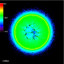
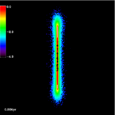
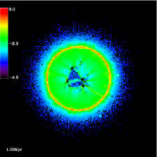
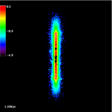
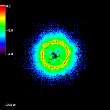
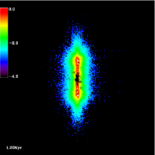
Figure 1.— The collapse of a sheet-like molecular cloud and the growth of the clumps in a simulation at 0, 0.2, 0.4, 0.6, 0.8, 1.2 Mpc. The left panel is the molecular cloud as viewed from the top, and the left panel from the side. Each box is 4.8 by 4.8 pc. The colors correspond to the logarithm of column density in $\rm{g~{}cm}^{-2}$.

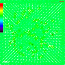
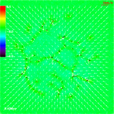
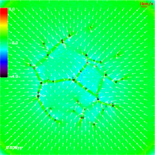
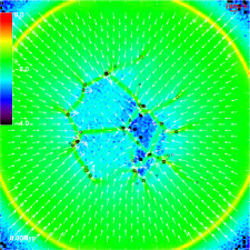
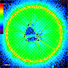
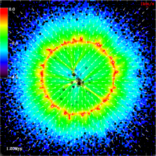
Figure 2.— The same simulation as in Figure 1, but only the inner part is shown. Each box is 2.4 pc by 2.4 pc. The arrows indicate the velocity vectors of the gas, with 1$\rm\,kms^{-1}$ marked on the upper right corner of each panel. The colors correspond to the log of column density in $\rm{g~{}cm}^{-2}$.

Figure 3.— The evolution of sink mass as a function of time in one of the runs of the equal mass case.

Figure 4.— The accretion rate vs. mass of sinks at 0.2, 0.4, 0.6, 0.8 and 1.0 Myr in one of the runs of equal mass sinks, with the uniform surface density cloud. The accretion rates for the higher-mass sinks follow $\dot{M}\propto M^{2}$.

Figure 5.— The accretion rate vs. distance of sink from the center of the sheet at t=0.2, 0.4, 0.6, 0.8, 1.0 and 1.2 My in the runs with equal mass sinks and the uniform surface density cloud. All 600 sinks from the six runs are included.

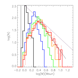
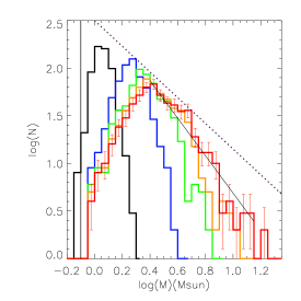
Figure 6.— Left: The distribution of mass at t=0.4, 0.6, 0.8, 1.0 and 1.2 Myr for the constant background density, equal clump mass case. The weighted linear fit has a slope of -2.08. Right: The distribution of mass at t = 0.4, 0.6, 0.8, 1.0 and 1.2 Myr for the varying background density, equal clump mass case. The weighted linear fit has a slope of $-\Gamma$ = -1.95. The dotted lines represent the Salpeter slope $-\Gamma$ = -1.35 (see Table 1).

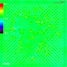
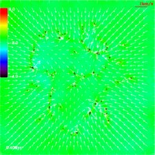
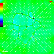
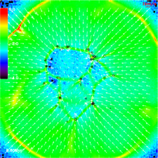
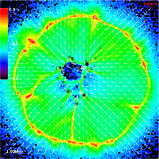
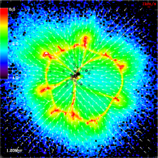
Figure 7.— The top view of the inner part (each box is 2.4 by 2.4 pc) of the case with equal clump mass and background density fluctuation. The arrows indicate the velocity vectors of the gas, with 1$\rm\,kms^{-1}$ marked on the upper right corner of each panel. The colors correspond to the log of column density in $\rm{g~{}cm}^{-2}$.

Figure 8.— The accretion rate vs. mass of sinks at 0.2, 0.4, 0.6, 0.8 and 1.0 Myr in one of the runs of the fluctuating background case. The accretion rates for the higher-mass sinks follow $\dot{M}\propto M^{2}$; the surface density fluctuations have little effect (see Figure 4 for comparison).

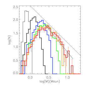
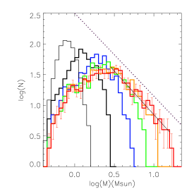
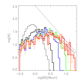
Figure 9.— Resulting mass distributions for initial clump masses with Gaussian distributions (Top left: $\sigma=0.05$; top right: $\sigma=0.1$; bottom left: $\sigma=0.2$) with constant background density. The linear fit slopes are $-\Gamma$ = -1.66, -1.42 and -1.03, respectively. The thin solid lines represent the initial clump mass distribution. The dotted lines represent the Salpeter slope $-\Gamma$ = -1.35.

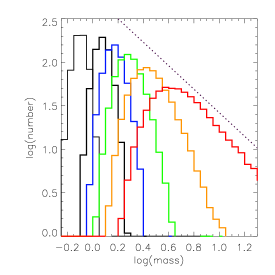
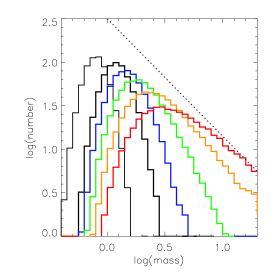
Figure 10.— The mass distribution at different time for $\dot{M}=\alpha M^{2}$. The top figure has a narrower initial mass range ($\sigma$ = 0.05 dex) than the bottom figure($\sigma$ = 0.1 dex). The thin solid line represents the initial distribution of masses, and the colored lines represent the mass distribution in increments of $0.16t_{\infty}=(\alpha M_{0})^{-1}$. The dotted line represent the Salpeter slope $-\Gamma$ = -1.35.

Figure 11.— Mass of sinks vs. the gas properties around the sinks for all the cases in the equal initial mass, uniform density case at t = 0.6Myr. The gas properties are evaluated at $R_{acc}=2GM/c_{s}^{2}$ from each sink. Top left: mass vs. gas velocity relative to the sink, top right: mass vs. gas density, middle left: mass vs. surface density, middle right: mass vs. surface density/velocity, bottom left: mass vs. $\rho/v^{3}$. There is no obvious correlation between the gas properties and the sink mass.

Figure 12.— Mass of sinks vs. the gas properties around the sinks for all the cases in the equal initial mass, uniform density case at t = 0.6Myr. The gas properties are evaluated at $R=c_{s}\times 0.1Myr=0.024$ pc from each sink. Top left: mass vs. gas velocity relative to the sink, top right: mass vs. gas density, middle left: mass vs. surface density, middle right: mass vs. surface density/velocity, bottom left: mass vs. $\rho/v^{3}$. There is no obvious correlation between the gas properties and the sink mass.

References

- Bastian et al. (2010) Bastian, N., Covey, K. R., & Meyer, M. R. 2010, ArXiv e-prints
- Bate (2009) Bate, M. R. 2009, MNRAS, 397, 232
- Bate et al. (2003) Bate, M. R., Bonnell, I. A., & Bromm, V. 2003, MNRAS, 339, 577
- Bate et al. (1995) Bate, M. R., Bonnell, I. A., & Price, N. M. 1995, MNRAS, 277, 362
- Bondi & Hoyle (1944) Bondi, H. & Hoyle, F. 1944, MNRAS, 104, 273
- Bonnell et al. (2001a) Bonnell, I. A., Bate, M. R., Clarke, C. J., & Pringle, J. E. 2001a, MNRAS, 323, 785
- Bonnell et al. (2003) Bonnell, I. A., Bate, M. R., & Vine, S. G. 2003, MNRAS, 343, 413
- Bonnell et al. (2001b) Bonnell, I. A., Clarke, C. J., Bate, M. R., & Pringle, J. E. 2001b, MNRAS, 324, 573
- Bonnell et al. (2007) Bonnell, I. A., Larson, R. B., & Zinnecker, H. 2007, in Protostars and Planets V, ed. B. Reipurth, D. Jewitt, & K. Keil, 149
- Burkert & Hartmann (2004) Burkert, A. & Hartmann, L. 2004, ApJ, 616, 288
- Chabrier (2003) Chabrier, G. 2003, PASP, 115, 763
- Clark et al. (2009) Clark, P. C., Glover, S. C. O., Bonnell, I. A., & Klessen, R. S. 2009, ArXiv e-prints
- Clarke (2009) Clarke, C. J. 2009, Ap&SS, 324, 121
- Hartmann et al. (2001) Hartmann, L., Ballesteros-Paredes, J., & Bergin, E. A. 2001, ApJ, 562, 852
- Heitsch & Hartmann (2008) Heitsch, F. & Hartmann, L. 2008, ApJ, 689, 290
- Heitsch et al. (2008a) Heitsch, F., Hartmann, L. W., & Burkert, A. 2008a, ApJ, 683, 786
- Heitsch et al. (2008b) Heitsch, F., Hartmann, L. W., Slyz, A. D., Devriendt, J. E. G., & Burkert, A. 2008b, ApJ, 674, 316
- Heitsch et al. (2006) Heitsch, F., Slyz, A. D., Devriendt, J. E. G., Hartmann, L. W., & Burkert, A. 2006, ApJ, 648, 1052
- Hennebelle & Chabrier (2008) Hennebelle, P. & Chabrier, G. 2008, ApJ, 684, 395
- Jappsen et al. (2005) Jappsen, A., Klessen, R. S., Larson, R. B., Li, Y., & Mac Low, M. 2005, A&A, 435, 611
- Klein et al. (2007) Klein, R. I., Inutsuka, S., Padoan, P., & Tomisaka, K. 2007, in Protostars and Planets V, ed. B. Reipurth, D. Jewitt, & K. Keil, 99–116
- Klessen & Burkert (2001) Klessen, R. S. & Burkert, A. 2001, ApJ, 549, 386
- Klessen et al. (2000) Klessen, R. S., Heitsch, F., & Mac Low, M. 2000, ApJ, 535, 887
- Kroupa & Weidner (2003) Kroupa, P. & Weidner, C. 2003, ApJ, 598, 1076
- Kroupa & Weidner (2005) Kroupa, P. & Weidner, C. 2005, in Astrophysics and Space Science Library, Vol. 327, The Initial Mass Function 50 Years Later, ed. E. Corbelli, F. Palla, & H. Zinnecker, 175
- Lada & Lada (2003) Lada, C. J. & Lada, E. A. 2003, ARA&A, 41, 57
- Padoan & Nordlund (2002) Padoan, P. & Nordlund, Å. 2002, ApJ, 576, 870
- Padoan et al. (2007) Padoan, P., Nordlund, Å., Kritsuk, A. G., Norman, M. L., & Li, P. S. 2007, ApJ, 661, 972
- Proszkow et al. (2009) Proszkow, E., Adams, F. C., Hartmann, L. W., & Tobin, J. J. 2009, ApJ, 697, 1020
- Rybicki (1971) Rybicki, G. B. 1971, Ap&SS, 14, 15
- Salpeter (1955) Salpeter, E. E. 1955, ApJ, 121, 161
- Springel (2005) Springel, V. 2005, MNRAS, 364, 1105
- Springel et al. (2001) Springel, V., Yoshida, N., & White, S. D. M. 2001, New Astronomy, 6, 79
- Tan et al. (2006) Tan, J. C., Krumholz, M. R., & McKee, C. F. 2006, ApJ, 641, L121
- Tobin et al. (2009) Tobin, J. J., Hartmann, L., Furesz, G., Mateo, M., & Megeath, S. T. 2009, ApJ, 697, 1103
- Vázquez-Semadeni et al. (2007) Vázquez-Semadeni, E., Gómez, G. C., Jappsen, A. K., Ballesteros-Paredes, J., González, R. F., & Klessen, R. S. 2007, ApJ, 657, 870
- Vázquez-Semadeni et al. (2006) Vázquez-Semadeni, E., Ryu, D., Passot, T., González, R. F., & Gazol, A. 2006, ApJ, 643, 245
- Zinnecker (1982) Zinnecker, H. 1982, New York Academy Sciences Annals, 395, 226