The Complete Four-Loop Four-Point Amplitude
in ${{\cal N}=4}$ Super-Yang-Mills Theory

Abstract

We present the complete four-loop four-point amplitude in ${{\cal N}=4}$ super-Yang-Mills theory, for a general gauge group and general $D$-dimensional covariant kinematics, and including all non-planar contributions. We use the method of maximal cuts — an efficient application of the unitarity method — to construct the result in terms of 50 four-loop integrals. We give graphical rules, valid in $D$-dimensions, for obtaining various non-planar contributions from previously-determined terms. We examine the ultraviolet behavior of the amplitude near $D=11/2$. The non-planar terms are as well-behaved in the ultraviolet as the planar terms. However, in the color decomposition of the three- and four-loop amplitude for an $SU(N_{c})$ gauge group, the coefficients of the double-trace terms are better behaved in the ultraviolet than are the single-trace terms. The results from this paper were an important step toward obtaining the corresponding amplitude in ${{\cal N}=8}$ supergravity, which confirmed the existence of cancellations beyond those needed for ultraviolet finiteness at four loops in four dimensions. Evaluation of the loop integrals near $D=4$ would permit tests of recent conjectures and results concerning the infrared behavior of four-dimensional massless gauge theory.

I Introduction

In recent years, scattering amplitudes have become an important tool for studying fundamental issues in gauge and gravity theories. For example, for the maximally supersymmetric four-dimensional super-Yang-Mills theory (${\cal N}=4$ sYM) in the planar limit, we have recently seen an all-order resummation ansatz proposed by Smirnov and two of the authors (BDS) ABDK ; BDS , strong-coupling results from Alday and Maldacena AldayMaldacena and the identification of of a new symmetry — dual (super) conformal invariance MagicIdentities ; DualConformal ; DualConformalWI . Together, these results have opened a new venue for studying the holographic AdS/CFT correspondence. Furthermore, they suggest the remarkable possibility that planar amplitudes of ${\cal N}=4$ sYM may ultimately be determined exactly AMOperatorProduct . In the maximally supersymmetric four-dimensional supergravity theory (${{\cal N}=8}$) CremmerJuliaScherk , the remarkable ultraviolet behavior of multi-loop graviton scattering amplitudes Finite ; GravityThree ; GravityFour ; BG2010 has challenged the widely-held belief that it is impossible to construct a perturbatively consistent point-like theory of quantum gravity.

In this paper we compute and analyze the four-loop four-point amplitude in ${\cal N}=4$ sYM, for an arbitrary non-abelian gauge group $G$. The amplitude can be graphically organized into planar and non-planar contributions. For the case of a special unitary gauge group, $G=SU(N_{c})$, the planar contributions dominate the limit in which the number of colors, $N_{c}$, tends to infinity. The planar terms are much simpler, and were computed previously BCDKS . The non-planar contributions are the subject of this paper.

Scattering amplitudes in gauge theory and gravity have a much richer structure than that revealed by Feynman diagrams. One striking example is Witten’s observation that tree amplitudes are supported on curves in twistor space WittenTopologicalString . At the multi-loop level, such structures have first been identified in theories with maximal supersymmetry. In ${\cal N}=4$ sYM, the first hint of powerful relations between higher- and lower-loop amplitudes was the “rung rule” relation BRY ; BDDPR for constructing particular contributions to four-point amplitudes. More remarkably, an iterative structure was uncovered in the dimensionally-regularized planar two-loop four-gluon amplitude ABDK , using the explicit values of the loop integrals in an expansion around $D=4$ SmirnovTwoloop . This iterative structure holds at three loops as well; it led to the all-loop BDS ansatz BDS for maximally-helicity-violating (MHV) amplitudes. For four external states, the ansatz is almost certainly correct, given its verification at strong coupling by Alday and Maldacena AldayMaldacena using the AdS/CFT correspondence. For four or five external legs, the assumption of dual conformal invariance, together with the structure of the infrared divergences, completely fixes the amplitudes’ dependence on the kinematics DualConformalWI , making it very likely that the BDS ansatz is correct. In addition, a variety of explicit four- and five-point computations confirm it through three loops in dimensional regularization ABDK ; BDS ; Iterate5pt ; SpradlinLeadingSingThreeLoop and with a Higgs regulator MassiveRegulatorProgress . However, for six or more external states, the BDS proposal is incomplete AMTrouble ; BLSV ; TwoLoopSixPt ; TwoLoopSixPtWilson . To clarify the structure of the additional “remainder” terms, it will undoubtedly be important to carry out further computations at both weak and strong coupling. Positive steps have been taken in this direction recently QMWL ; R6 ; AMNew ; AMOperatorProduct .

Much less is known about non-planar contributions to ${\cal N}=4$ sYM amplitudes. As a step in this direction, the principal aim of this paper is to construct the complete four-loop four-point amplitude in ${\cal N}=4$ sYM, including non-planar contributions, using the unitarity method UnitarityMethod and various refinements of it. We express the result in terms of 50 distinct loop momentum integrals, each with nontrivial numerators. (One of the 50 gives a contribution to the amplitude that vanishes after integration.) At three loops, the analogous expression requires only nine distinct integrals GravityThree ; CompactThree .

Using these representations of the three- and four-loop amplitudes, we can study their ultraviolet (UV) properties, in particular the critical dimension $D_{c}(L)$ in which the first UV divergence appears, as a function of the loop number $L$. Based on information from some of the unitarity cuts, a formula for $D_{c}(L)$ was suggested in ref. BDDPR (see eq. (41) below). This formula corresponds to counterterms in higher dimensions of the schematic form ${\cal D}^{2}F^{4}$, where $F$ is the Yang-Mills field strength, ${\cal D}$ is a covariant derivative, and the precise color structure is not yet specified. This form for the counterterms was later argued for by Howe and Stelle HoweStelleRevisited , based on harmonic superspace HarmonicSuperspace .

Here we confirm this expected behavior for the so-called single-trace terms in the amplitude for $G=SU(N_{c})$, which correspond to counterterms of the form $\,{\rm Tr}({\cal D}^{2}F^{4})$. However, we also find striking cancellations in the double-trace terms in the amplitude, starting at three loops, such that counterterms of the form $\,{\rm Tr}({\cal D}^{2}F^{2})\,{\rm Tr}(F^{2})$, etc., are absent. These results were first reported in refs. DurhamAndCopenhagenTalks . These cancellations have been discussed using the pure spinor formalism in string theory DoubleTraceBerkovits and field theory BG2010 , as well as from the point of view of algebraic non-renormalization theorems DoubleTraceNonrenormalization . Because of contamination from the closed-string sector, the string-based arguments apply only to the double-trace terms with the most factors of $N_{c}$, namely $N_{c}^{L-1}$; the field-theory arguments BG2010 are more general in this regard. Here we will rearrange the color structure of the amplitudes in order to make manifest the additional cancellations in the double-trace terms, including all powers in $N_{c}$, at three and four loops.

The present paper also provides the key input for the unitarity-based computation of the four-loop four-graviton amplitude GravityFour in ${{\cal N}=8}$ supergravity CremmerJuliaScherk . On general grounds, the unitarity cuts of gravity loop amplitudes can be obtained from those of Yang-Mills amplitudes BDDPR . In a first step, generalized unitarity allows gravity loop amplitudes to be decomposed into gravity tree amplitudes. Then the tree-level Kawai, Lewellen and Tye (KLT) relations KLT can be used to express the gravity tree amplitudes in terms of gauge-theory tree amplitudes. Alternatively, one can use the new diagrammatic numerator relations between gravity and gauge-theory tree amplitudes developed by three of the authors BCJ . Thus the gravity cuts are expressed as bilinear combinations of gauge-theory cuts. All the information needed for the gravity computation may be found by cutting the gauge-theory amplitude. In the case of ${{\cal N}=8}$ supergravity, all the sums over supersymmetric particles running in the loops are automatically performed in the course of the ${\cal N}=4$ sYM computation. Because gravity does not involve color, the non-planar contributions are just as important as the planar ones, and the full non-planar ${\cal N}=4$ sYM amplitude is required.

Multi-loop ${{\cal N}=8}$ supergravity amplitudes have revealed UV cancellations not anticipated from earlier superspace power-counting arguments. The explicit UV behavior of the three- and four-loop four-point amplitudes GravityThree ; GravityFour exhibits strong cancellations, beyond those needed for UV finiteness in four dimensions. Moreover, an analysis of certain unitarity cuts demonstrates the existence of novel higher-loop cancellations to all loop orders Finite , based on the one-loop “no-triangle property” OneloopMHVGravity ; NoTriangle ; NoTriangleSixPt ; NoTriangleKallosh ; BjerrumVanhove ; AHCKGravity . These results support the proposal that ${{\cal N}=8}$ supergravity might be a perturbatively UV finite theory of quantum gravity. String dualities DualityArguments and non-renormalization theorems Berkovits have also been used to argue for both UV finiteness of ${{\cal N}=8}$ supergravity, and for a delay in the onset of divergences, although difficulties with decoupling towers of massive states GOS and technical issues with the pure-spinor formalism GRV2010 ; Vanhove2010 ; BG2010 may affect these conclusions.

Another important reason to study the non-planar contributions to ${\cal N}=4$ sYM amplitudes is to investigate whether the resummation of the four-point amplitude to all loop orders ABDK ; BDS ; AldayMaldacena can be accomplished in some form for non-planar amplitudes as well. However, given the more complicated color structure of non-planar contributions, and the probable lack of integrability for subleading terms in the $1/N_{c}$ expansion, it is not clear whether such a generalization can exist. What is clear is that the infrared-singular behavior would have to be understood first, before the behavior of infrared-finite terms could be addressed. At subleading orders in $1/N_{c}$, the soft anomalous dimension matrix ${\bf\Gamma}_{S}$ controls infrared singularities due to soft-gluon exchange SoftMatrix ; KorchemskyRadyushkin . The matrix structure becomes trivial in the planar, or large-$N_{c}$, limit BDS .

Surprisingly, the two-loop soft anomalous dimension matrix in massless gauge theory is proportional to the one-loop one TwoLoopSoftMatrix . The proportionality constant is determined by the cusp anomalous dimension KorchemskyRadyushkin . This result was later understood to be a consequence of an anomalous symmetry of Wilson-line expectation values under the rescaling of their velocities BN ; GM . It has been conjectured CompactThree ; BN ; GM that the proportionality might persist to all loop orders. However, velocity rescaling alone, even combined with other constraints, such as collinear factorization of amplitudes TwoLoopSplit ; BN , is not powerful enough to determine the form of ${\bf\Gamma}_{S}$ beyond two loops DGM , except for the matter-dependent part at three loops Matter3l . In principle, the soft anomalous dimension matrix for ${\cal N}=4$ sYM can be determined at three and four loops, for the case of four external massless states, using the results in ref. CompactThree and in this paper. At three loops, this computation would also determine ${\bf\Gamma}_{S}$ for any massless gauge theory, because the matter-dependent part is known Matter3l .

To perform such a determination, the dimensionally-regularized loop integrals entering the amplitudes, for $D=4-2\epsilon$, would have to be expanded in a Laurent series around $\epsilon=0$. If this can be accomplished, then it is relatively straightforward to compare the results with fixed-order formulæ STY ; TwoLoopSoftMatrix in order to extract ${\bf\Gamma}_{S}$. The Laurent series for the $L$-loop amplitude begins at order $1/\epsilon^{2L}$, and the $L$-loop soft anomalous dimension matrix first enters at order $1/\epsilon$ in the expansion.

At order $1/\epsilon^{2}$, the $L$-loop cusp anomalous dimension $\gamma_{K}^{(L)}$ appears. While this quantity is known in the planar limit of ${\cal N}=4$ sYM through at least four loops BCDKS ; CSVcusp4l , and very likely to all loop orders BES , the subleading-color terms are not known beyond three loops. If they are nontrivial at four loops, it would indicate the violation of “quadratic Casimir scaling”, or $\gamma_{K}^{(L)}\,\propto\,N_{c}^{L}$ for $G=SU(N_{c})$, which holds through three loops MVV . Such a violation is allowed by group theory, beginning at four loops, and hinted at by strong-coupling considerations Armoni . However, it would be very useful to compute the subleading-color terms in $\gamma_{K}^{(4)}$ explicitly, as it has been conjectured that quadratic Casimir scaling will continue to hold beyond three loops BN .

Unfortunately, both these tests will have to await improved techniques for the evaluation of the Laurent expansion in $\epsilon$ of three- and higher-loop non-planar integrals. The non-planar integrals required for three-loop form factors (one off-shell leg and two on-shell massless ones) have been evaluated ThreeLoopNonPlanarIntegrals , but not yet those for on-shell scattering of four massless states at three loops (let alone four loops).

In order to determine the four-loop amplitude in terms of a set of loop integrals, we use the unitarity method UnitarityMethod , in particular the information provided by generalized unitarity cuts GeneralizedUnitarity ; TwoLoopSplit ; BCFGeneralized ; FiveLoop . The unitarity method takes advantage of the fact that tree-level amplitudes are much simpler than individual Feynman diagrams. One can exploit structures that are obscure in Feynman diagrams but visible in on-shell amplitudes.

For planar ${\cal N}=4$ sYM, the observation that the loop amplitudes can be expressed in terms of a restricted set of “pseudoconformal” integrals MagicIdentities ; BCDKS ; FiveLoop ; KorchemskyZeros helps streamline the construction of a candidate expression, or ansatz, that is consistent with the unitarity cuts. For a planar graph, dual coordinates $x_{i}$ can be associated with nodes of the dual graph; differences of pairs of $x_{i}$ are identified with momenta of the internal or external lines of the original graph. Loosely speaking, pseudoconformal integrals are integrals that are invariant under conformal transformations of the dual coordinates. It has not yet been proven that all planar loop amplitudes in ${\cal N}=4$ sYM are expressible in terms of pseudoconformal integrals (especially for non-MHV helicity configurations for six or more external states). However, in any given loop amplitude we can directly confirm that no other integrals appear, once the pseudoconformal ansatz satisfies all the unitarity cuts. This observation helped simplify recent calculations of the planar five-loop four-point FiveLoop and two-loop six-point TwoLoopSixPt MHV amplitudes in ${\cal N}=4$ sYM.

In contrast, for non-planar terms in the amplitude, there is currently no useful definition of dual conformal symmetry. In addition, non-planar contributions are inherently more intricate than planar ones. Nevertheless, planar and non-planar contributions do appear to be linked via identities between diagram numerators, whose structure is similar to the Jacobi identity obeyed by color factors BCJ ; BCJOther ; Square . Very recently, this structure has been observed to hold at the three-loop level, with no cut conditions imposed BCJLoop . Indeed, for the three-loop four-point amplitude in ${\cal N}=4$ sYM, one of the planar diagrams is sufficient for determining all the non-planar ones. It would be interesting to study these properties further, in particular to determine the restrictions they place on the four-loop amplitude presented here. We leave this interesting question to the future.

A powerful way to determine large classes of both planar and non-planar contributions is through graphical rules that capture some of the features of generalized unitarity cuts. The first of these rules is the rung rule BRY ; BDDPR . The Jacobi-like relation between planar and non-planar contributions can also be implemented as a graphical manipulation BCJ . There is also a “box-substitution rule” FiveLoop , which we will generalize here. Some related graphical identities may be found in ref. CachazoSkinner . The rules given here reduce the determination of contributions containing four-point subdiagrams to a few simple manipulations.

The graphical rules presented in this paper capture many contributions, but not all of them. In order to determine the missing ones, we used the method of maximal cuts FiveLoop ; CompactThree . For four-point amplitudes in $D\geq 4$, maximal cuts are those generalized unitarity cuts in which only three-point tree amplitudes appear, connected by cut propagators, i.e., they contain the maximum number of cut propagators. One first constructs a candidate expression (ansatz) for the loop amplitude that is equal to each maximal cut, when evaluated for the appropriate cut kinematics. We refer to this procedure as “matching” the ansatz to the maximal cuts. Next one adjusts the ansatz to match as well the next-to-maximal cuts in which a cut propagator is removed from between two of the three-point trees to form a four-point tree. This captures all contributions with a single four-point vertex, or “contact term”. Then one matches to further near-maximal cuts with more canceled propagators.

In order to construct the complete four-loop amplitude, we used a large number of maximal and near-maximal cuts. To ensure that no contributions were dropped, we then evaluated a set of 13 “basis cuts” (not counting permutations of legs) which suffice to determine any massless four-loop four-point amplitude. We verified that our answer matches all of these cuts. Many of the cuts were evaluated using four-dimensional intermediate momenta, so that powerful helicity and supersymmetry methods could be exploited. This leaves open the possibility that some terms could be missed, which vanish when the cut momenta are restricted to four dimensions. For this reason, we performed a large number of consistency checks, as described in section II.2.

The unitarity method also allows us to use an on-shell superspace formalism to sum over states crossing cuts. On-shell superspaces involve only physical states and, for our purpose, they are generally far simpler than their off-shell cousins. A number of years ago Nair presented an on-shell superspace Nair for MHV tree amplitudes in ${\cal N}=4$ sYM. More recently, this superspace has been extended to any helicity and particle configuration. For the computations of this paper we follow the MHV generating-function approach GGK ; FreedmanGenerating ; FreedmanUnitarity , as organized in ref. SuperSum for use in multi-loop calculations. We also exploit specific super-sum results for cuts involving next-to-MHV tree amplitudes FreedmanUnitarity . A related procedure AHCKGravity ; RecentOnShellSuperSpace ; KorchemskyOneLoop for covering any helicity and particle content employs the momentum shifts used by Britto, Cachazo, Feng and Witten to derive on-shell recursion relations BCFW , extended to shifts of anti-commuting parameters. One-loop examples that use an on-shell superspace in conjunction with the unitarity method may be found in refs. FreedmanGenerating ; KorchemskyOneLoop ; AHCKGravity . Various higher-loop examples, including four-loop ones, are given in refs. FreedmanUnitarity ; SuperSum .

This paper is organized as follows. In section II we describe the general structure of multi-loop amplitudes. We also recall the specific form of four-point amplitudes in ${\cal N}=4$ sYM from one to three loops, as well as the planar terms at four loops. We give a brief overview of the techniques used to determine the amplitudes. In section III we describe in more detail various tools for determining the non-planar contributions. In section IV we present the complete four-loop four-point amplitude in terms of a set of 50 integrals. The ultraviolet divergence properties of the four-point amplitude through four loops, in the critical dimension $D_{c}(L)$, are discussed in section V. In section VI we compute the leading UV divergence for the double-trace terms at three loops, which appears at $D=20/3$ (in contrast to the single-trace terms, which first diverge in $D_{c}(3)=6$). In section VII, we give our conclusions and prospects for the future. In appendix A, we present a sample evaluation of a nontrivial non-planar cut. In appendix B we provide various representations of the color factors appearing in the amplitudes. In appendix C we collect the numerator and color factors for the 50 integrals entering the four-loop amplitude.

II Structure of multi-loop amplitudes

Loop amplitudes in ${\cal N}=4$ sYM exhibit remarkable simplicity for a gauge theory. Using the unitarity method UnitarityMethod , a large variety of amplitudes have been constructed through five loops BRY ; BDDPR ; BCDKS ; FiveLoop ; Iterate5pt ; TwoLoopSixPt ; LeadingSingularityCalcs ; SpradlinLeadingSingThreeLoop in terms of loop-momentum integrals. Indeed, the structure of the planar four-point amplitude is simple enough that an all-loop order resummation is possible BDS ; AldayMaldacena . This simplicity in the planar sector has been understood in terms of a new symmetry dubbed “dual conformal symmetry” MagicIdentities ; KorchemskyZeros ; DualConformal , which is intimately connected to integrability AmplitudeIntegrability . In this paper we focus on the non-planar contributions to ${\cal N}=4$ sYM amplitudes. Although they are much more intricate and less well understood than the planar amplitudes, their structure is still remarkably simple, especially when compared to amplitudes in theories with fewer supersymmetries.

In this section we begin by describing the color and parent-graph organization of multi-loop amplitudes, including a review of the results for the lower-loop and planar four-loop four-point amplitudes in ${\cal N}=4$ sYM. Then we turn to a brief review of the unitarity method.

II.1 Color and parent-graph decomposition

For gauge group $G=SU(N_{c})$, the leading-color (planar) terms are particularly simple. They have essentially the same color structure as the corresponding tree amplitudes. The leading-in-$N_{c}$ contribution to the $L$-loop $n$-point amplitude may be written as,

$${\cal A}_{n}^{(L),\,{\rm Planar}}=g^{n-2}\Biggl{[}{g^{2}N_{c}\over(4\pi)^{2-\epsilon}}\Biggr{]}^{L}\hskip-5.69054pt\sum_{\sigma\in S_{n}/Z_{n}}\hskip-5.69054pt\,{\rm Tr}(T^{a_{\sigma(1)}}\ldots T^{a_{\sigma(n)}})A_{n}^{(L)}(\sigma(1),\sigma(2),\ldots,\sigma(n))\,,$$ (1)

where the $T^{a_{i}}$ are generators in the fundamental representation of $SU(N_{c})$, with adjoint color indices $a_{i}$, and the sum runs over non-cyclic permutations of the external legs. In this expression we have suppressed the (all-outgoing) momenta $k_{i}$, as well as polarizations and particle types, leaving only the integer index $i$ as a collective label. This decomposition holds for all particles in the gauge super-multiplet, as they are all in the adjoint representation. The color-ordered (or color-stripped) partial amplitudes $A_{n}^{(L)}$ carry no color indices; they depend only on the kinematics, polarizations and particle type. At leading order in the $1/N_{c}$ expansion they can be expressed solely in terms of planar loop integrals.

For the complete amplitude for a general gauge group $G$, including all non-planar contributions, the parent-graph decomposition,

$${\cal A}_{n}^{(L)}=g^{2L+n-2}\sum_{i\,\in\,{\rm parent}}a_{i}C_{i}I_{i}\,,$$ (2)

is more convenient than the color-trace representation. The parent graphs are cubic graphs — graphs containing only three-point vertices. Momentum is conserved at each vertex. Every graph specifies simultaneously a combinatorial factor $a_{i}$, a color dressing $C_{i}$ and a Feynman loop integral $I_{i}$.

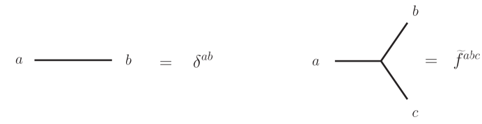
Figure 1: Rules for obtaining the color factors associated with cubic parent graphs. The roman letters $a,b,c$ are color indices. The sign of each structure constant $\tilde{f}^{abc}$ is fixed by the clockwise ordering of each vertex, as drawn.

The $C_{i}$ are written in terms of group structure constants. The contractions of group indices are encoded by the graph $i$ using the rules given in fig. 1. More precisely, the color factors $C_{i}$ are obtained by dressing each three-vertex of the parent graph with structure constants, normalized as,

$$\tilde{f}^{abc}=i\sqrt{2}f^{abc}=\,{\rm Tr}([T^{a},T^{b}]T^{c})\,,$$ (3)

where $f^{abc}$ are the standard structure constants of the gauge group $G$, and the hermitian generators $T^{a}$ are normalized via $\,{\rm Tr}(T^{a}T^{b})=\delta^{ab}$. The $\tilde{f}^{abc}$ should follow the clockwise ordering of the legs for each vertex of the parent graph. This clockwise ordering is important. For example, if one redraws a graph so that an odd number of three-point vertices have their ordering reversed, then the signs of both $C_{i}$ and $I_{i}$ should be flipped in tandem.

Each parent integral for the $L$-loop four-point amplitude is a Feynman integral with the following general structure and normalization,

$$I_{i}=(-i)^{L}\int\biggl{(}\prod_{j=1}^{L}\frac{d^{D}\ell_{j}}{(2\pi)^{D}}\biggr{)}\,\frac{N_{i}(\ell_{j},k_{m})}{\prod_{n=1}^{3L+1}l_{n}^{2}}\,,$$ (4)

where $k_{m}$, $m=1,2,3$, are the three independent external momenta, $\ell_{j}$ are the $L$ independent loop momenta, and $l_{n}$ are the momenta of the $(3L+1)$ propagators (internal lines of the graph $i$), which are linear combinations of the $\ell_{j}$ and the $k_{m}$. As usual, $d^{D}\ell_{j}$ is the $D$-dimensional measure for the $j^{\rm th}$ loop momentum. The numerator polynomial $N_{i}(\ell_{j},k_{m})$ is a polynomial in both internal and external momenta.

Unlike the decomposition using color traces, the parent-graph decomposition is not unique, due to contact terms. Contact terms are contributions to the amplitude that lack one or more propagators, relative to the parent graphs. If the contact terms were allowed to contribute as isolated integrals, they would correspond to graphs containing quartic or higher-order vertices. Here we will absorb all contact terms into parent integrals, by multiplying and dividing by the missing propagator or propagators, so that the corresponding term in $N_{i}(\ell_{j},k_{m})$ will contain factors of $l_{n}^{2}$, which we refer to as inverse propagators. However, because the associated color factors $C_{i}$ can be expressed as linear combinations of other color factors via the Jacobi identities, there is an ambiguity in choosing the specific parent graph to absorb a given contact term. Although there are many valid choices, particular choices can reveal nontrivial structures or symmetries.

For ${\cal N}=4$ sYM amplitudes, the freedom in assigning contact terms to parent graphs can be exploited to remove all graphs with nontrivial two- or three-point subgraphs, as was done at three loops CompactThree . While supersymmetry and gauge invariance may be used to show the all-order consistency of this condition on the parent graphs, a more direct approach was taken in ref. CompactThree , by verifying that an ansatz in this class is compatible with all unitarity cuts. Here we will take the same approach at four loops.

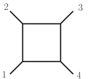
Figure 2: The box diagram is the only parent graph at one loop (up to permutations of the external legs).

At one loop, the structure of the ${\cal N}=4$ sYM four-point amplitude is especially simple. We modify eq. (2) slightly by extracting an overall prefactor, and write the result as,

$${\cal A}_{4}^{(1)}\! = \!-{1\over 8}g^{4}\,{\cal K}\,\sum_{S_{4}}\,C^{\rm box}_{1234}\,I^{\rm box}(s_{12},s_{23})\,,\hskip 8.5359pt$$ (5)

where $g$ is the gauge coupling. The prefactor ${\cal K}$ is defined by

$${\cal K}\equiv{\cal K}(1,2,3,4)\equiv s_{12}\,s_{23}\,A_{4}^{{\rm tree}}(1,2,3,4)\,,$$ (6)

where $s_{12}=(k_{1}+k_{2})^{2}$, $s_{23}=(k_{2}+k_{3})^{2}$, and the $k_{i}$ are the external momenta. It contains all information about the four external states.

The unique parent graph at one loop is the box diagram shown in fig. 2. For external legs ordered 1234, the box color factor is

$$C^{\rm box}_{1234}=\tilde{f}^{a_{1}a_{6}a_{5}}\tilde{f}^{a_{2}a_{7}a_{6}}\tilde{f}^{a_{3}a_{8}a_{7}}\tilde{f}^{a_{4}a_{5}a_{8}}\,,$$ (7)

where we sum over repeated indices. This form is valid for any gauge group. Finally, $I^{\rm box}(s_{12},s_{23})$ is the one-loop box integral,

$$I^{\rm box}(s_{12},s_{23})=-i\int{d^{D}p\over(2\pi)^{D}}{1\over p^{2}(p-k_{1})^{2}(p-k_{1}-k_{2})^{2}(p+k_{4})^{2}}\,.$$ (8)

The sum in eq. (5) runs over the 24 permutations of external legs $\{1,2,3,4\}$, denoted by $S_{4}$. The permutations act on both the momentum and color labels. The prefactor of $1/8$ accounts for an eightfold overcount in the permutation sum, which we leave in to make it slightly easier to generalize to higher loops.

In eq. (6), $A_{4}^{\rm tree}(1,2,3,4)$ stands for any ${\cal N}=4$ sYM tree amplitude in the canonical color order. In four dimensions, a compact form of this object can be written down using anti-commuting parameters $\eta$ in the on-shell superspace formalism Nair ; GGK ; FreedmanGenerating ; RecentOnShellSuperSpace ; KorchemskyOneLoop ; AHCKGravity ; FreedmanUnitarity ,

$$A_{4}^{{\rm tree}}(1,2,3,4)\bigr{|}_{D=4} = {i\delta^{(8)}(\lambda_{1}\eta_{1}+\lambda_{2}\eta_{2}+\lambda_{3}\eta_{3}+\lambda_{4}\eta_{4})\over\left\langle 1\,2\right\rangle\left\langle 2\,3\right\rangle\left\langle 3\,4\right\rangle\left\langle 4\,1\right\rangle}\,,$$ (9)

$${\cal K}(1,2,3,4)\bigr{|}_{D=4} = -i\,{\left[1\,2\right]\left[3\,4\right]\over\left\langle 1\,2\right\rangle\left\langle 3\,4\right\rangle}\,\delta^{(8)}(\lambda_{1}\eta_{1}+\lambda_{2}\eta_{2}+\lambda_{3}\eta_{3}+\lambda_{4}\eta_{4})\,.$$ (10)

It is not difficult to verify that $(\left[1\,2\right]\left[3\,4\right])/(\left\langle 1\,2\right\rangle\left\langle 3\,4\right\rangle)$ is symmetric under exchange of any two legs, and that ${\cal K}$ is local. Related to this, ${\cal K}$ represents the color-stripped four-point (linearized) matrix elements of the local operator $\,{\rm Tr}F^{4}$, plus its supersymmetric partners. Therefore ${\cal K}$ is a natural prefactor to extract from the four-point amplitude in ${\cal N}=4$ sYM.

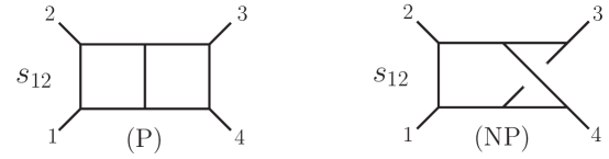
Figure 3: The planar and non-planar parent graphs contributing to the two-loop four-point amplitude. The prefactors $s_{12}$ are the integral numerators $N^{({\rm P})}$ and $N^{({\rm NP})}$, respectively.

At two loops, the full ${\cal N}=4$ sYM amplitude is given by a similar permutation sum as for the one-loop case (5) BRY ; BDDPR ,

$${\cal A}_{4}^{(2)}\! = \!{1\over 4}g^{6}\,{\cal K}\,\sum_{S_{4}}\,\Bigl{[}C^{\rm(P)}_{1234}\,I^{\rm(\rm P)}(s_{12},s_{23})\,+\,C^{\rm(NP)}_{1234}\,I^{\rm(NP)}(s_{12},s_{23})\Bigr{]}\,.\hskip 8.5359pt$$ (11)

The planar and non-planar double-box integrals, displayed in fig. 3, are defined by

$$\hskip-8.5359ptI^{\rm(P)}(s_{12},s_{23})\! = \!(-i)^{2}\!\int{d^{D}pd^{D}q\over(2\pi)^{2D}}\,{s_{12}\over p^{2}\,(p-k_{1})^{2}\,(p-k_{12})^{2}\,(p+q)^{2}q^{2}\,(q-k_{4})^{2}\,(q-k_{34})^{2}}\,,\hskip 8.5359pt$$

$$\hskip-8.5359ptI^{\rm(NP)}(s_{12},s_{23})\! = \!(-i)^{2}\!\int{d^{D}pd^{D}q\over(2\pi)^{2D}}\,{s_{12}\over p^{2}(p-k_{4})^{2}(p+q)^{2}(p+q+k_{3})^{2}q^{2}(q-k_{1})^{2}(q-k_{12})^{2}}\,,$$

with $k_{12}=k_{1}+k_{2}$ and $k_{34}=k_{3}+k_{4}$. The permutation sum again runs over $S_{4}$ and acts on both momentum and color labels. Because both graphs in fig. 3 have a fourfold symmetry, the permutation sum overcounts by a factor of four. As before, we include this overcount and divide by an overall symmetry factor. In a form valid for any gauge group, the color factors of the planar and non-planar graphs, with legs ordered 1234, are,

$$C^{(\rm P)}_{1234} = \tilde{f}^{a_{1}a_{6}a_{5}}\tilde{f}^{a_{2}a_{7}a_{6}}\tilde{f}^{a_{3}a_{9}a_{8}}\tilde{f}^{a_{4}a_{10}a_{9}}\tilde{f}^{a_{7}a_{8}a_{11}}\tilde{f}^{a_{5}a_{11}a_{10}}\,,$$

$$C^{(\rm NP)}_{1234} = \tilde{f}^{a_{1}a_{6}a_{5}}\tilde{f}^{a_{2}a_{7}a_{6}}\tilde{f}^{a_{3}a_{9}a_{8}}\tilde{f}^{a_{4}a_{11}a_{10}}\tilde{f}^{a_{7}a_{8}a_{10}}\tilde{f}^{a_{5}a_{9}a_{11}}\,.$$ (13)

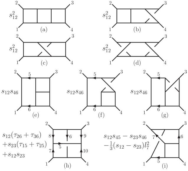
Figure 4: The nine parent graphs for the three-loop four-point ${\cal N}=4$ sYM amplitude. The prefactor of each diagram is the numerator polynomial $N^{(x)}$. The kinematic invariants are defined in eq. (15).

At three loops, the fully color-dressed three-loop four-point ${\cal N}=4$ sYM amplitude is given by GravityThree ; CompactThree ,

$${\cal A}_{4}^{(3)}\! = \!-{1\over 4}\,g^{8}\,{\cal K}\,\sum_{S_{4}}\,\Bigl{[}C^{\rm(a)}I^{\rm(a)}+C^{\rm(b)}I^{\rm(b)}+{\textstyle{1\over 2}}C^{\rm(c)}I^{\rm(c)}+{\textstyle{1\over 4}}C^{\rm(d)}I^{\rm(d)}$$ (14)

$$\hbox{}\hskip 56.9055pt+2C^{\rm(e)}I^{\rm(e)}+2C^{\rm(f)}I^{\rm(f)}+4C^{\rm(g)}I^{\rm(g)}+{\textstyle{1\over 2}}C^{\rm(h)}I^{\rm(h)}+2C^{\rm(i)}I^{\rm(i)}\Bigr{]}\,.\hskip 8.5359pt$$

In this case, the integrals $I^{(x)}(s_{12},s_{23})$ are $D$-dimensional loop integrals corresponding to the nine graphs shown in fig. 4, using eq. (4) with the numerator polynomials $N_{i}$ displayed next to the diagrams. In fig. 4 the (outgoing) momenta of the external legs are denoted by $k_{i}$ with $i=1,2,3,4$, while the momenta of the internal legs are denoted by $l_{i}$ with $i>4$. For convenience we use the following shorthand notation,

$$s_{ij}=\left\{\begin{array}[]{ll}(k_{i}+k_{j})^{2}&\hskip 28.45274pti,j\leq 4\\ (k_{i}+l_{j})^{2}&\hskip 28.45274pti\leq 4<j\\ (l_{i}+l_{j})^{2}&\hskip 28.45274pt4<i,j\end{array}\right\}\,,\hskip 56.9055pt\tau_{ij}=2k_{i}\cdot l_{j}\,.$$ (15)

In the three-loop case, some of the numerator polynomials contain squares of loop momenta, which could be used to collapse propagators and generate contact terms. (The three-loop four-graviton amplitude in ${{\cal N}=8}$ supergravity can be written CompactThree in a form very similar to eq. (14), except that there are no color factors, and the numerator factors in the loop integrals are of course different.)

The color factor associated with each integral in the three-loop amplitude is easy to write down from the parent graph, following fig. 1. The expression (14) is valid for any gauge group $G$ and any dimension $D$, as verified by a direct evaluation of the color-dressed cuts CompactThree .

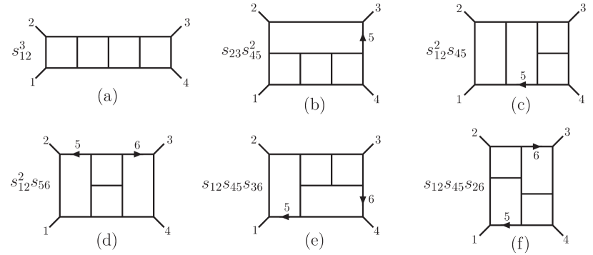
Figure 5: Planar contributions to the four-loop four-point amplitude.

Figure 6: Contact terms in the planar four-point amplitude, which can be absorbed into the numerator of graph (f) of fig. 5. (Note that here (f₂) and (d₂) refers to the labeling used in ref. BCDKS ; unlike ref. BCDKS we choose to write out explicitly the relative factors of these integrals with respect to diagram (f).)

In section IV we will present the complete four-loop four-point amplitude of ${\cal N}=4$ sYM, using the same type of parent-graph decomposition. As we will demonstrate, this amplitude can be decomposed into 50 distinct parent integrals, corresponding to cubic graphs with no nontrivial two- or three-point subgraphs. As explained earlier, contact terms are incorporated as numerator factors containing inverse propagators. Thus we write the four-loop four-point amplitude as,

$${\cal A}_{4}^{(4)}=g^{10}\,{\cal K}\,\sum_{S_{4}}\sum_{i=1}^{50}a_{i}C_{i}I_{i}\,,$$ (16)

where the usual prefactor ${\cal K}$ is common to all terms, the $a_{i}$ are combinatoric symmetry factors and the $C_{i}$ color factors. The integrals $I_{i}$ are specified by the propagators associated with the parent graph, and by the numerator polynomials $N_{i}$. Each numerator polynomial is subject to various constraints. After accounting for the four powers of external momenta in ${\cal K}$ in eq. (16), dimensional analysis implies that the numerator polynomial $N_{i}(\ell_{j},k_{j})$ is of degree 6 in the momenta. Moreover, consistency with the known power-counting BDDPR ; HoweStelleRevisited requires that the numerator polynomials for ${\cal N}=4$ sYM have a maximum degree of 4 in the loop momenta.

The planar contributions to the four-loop four-point amplitude were presented earlier BCDKS , although they were given in the color-trace decomposition, rather than the graphical decomposition used here. Out of the eight different types of planar integrals present in the amplitude, the six parent graphs are shown in fig. 5. (The combinatoric factors are not included in the figure.) The two additional contributions are contact terms and are shown in fig. 6. A convenient choice for absorbing these contact terms is to assign both of them to the parent graph (f) of fig. 5, by incorporating inverse propagators in their numerators. The result, after combining two different permutations of diagram (f), can be found in fig. 22, diagram (28).

II.2 Unitarity method

The unitarity method provides an efficient framework for systematically constructing and verifying the expression for any massless multi-loop amplitude. This method, along with various refinements, has already been described in some detail elsewhere UnitarityMethod ; BDDPR ; GeneralizedUnitarity ; TwoLoopSplit ; BCFGeneralized ; FiveLoop ; CachazoSkinner . Here we summarize those points directly salient to our construction of multi-loop amplitudes in ${\cal N}=4$ sYM.

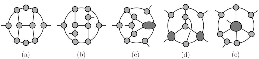
Figure 7: Examples of maximal and near-maximal cuts used to construct a complete ansatz for the four-loop ${\cal N}=4$ sYM amplitude. Cuts (a) and (b) have the maximal 13 cut conditions. Near-maximal cuts (c) have 12 conditions, and (d) and (e) have 11 conditions. No cuts with fewer than 11 on-shell propagators are needed to build the complete ansatz.

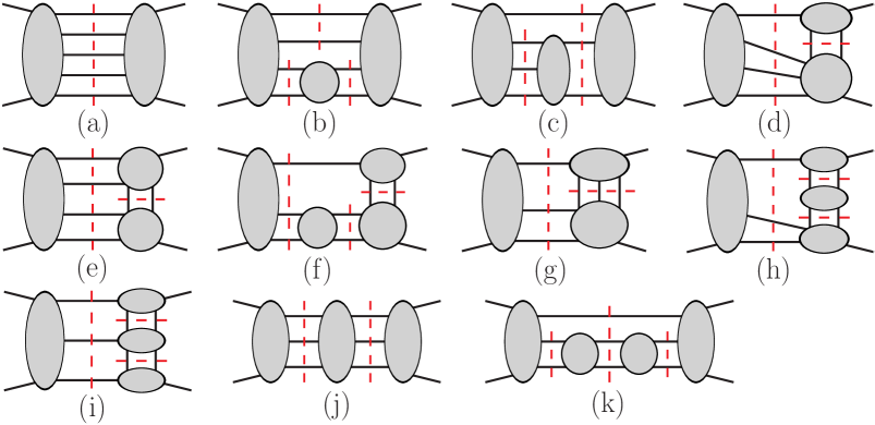
Figure 8: These 11 cuts, along with the two-particle cuts in fig. 9, suffice to determine any massless four-loop four-point amplitude. As displayed they determine any planar amplitude; to determine any non-planar contributions one must also include cuts with the legs of each tree sub-amplitude permuted arbitrarily. The cuts (h) and (k) have been evaluated in $D$ dimensions, as they are included in the box cuts fig. 10(c) and (e), respectively.

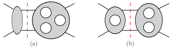
Figure 9: The two-particle cuts. These cuts have been evaluated in $D$ dimensions. Together with the cuts of fig. 8 these form a spanning set of cuts for any massless four-loop four-point amplitude.

A generalized unitarity cut is a sum over products of amplitudes,

$$i^{c}\sum_{\rm states}A_{(1)}A_{(2)}A_{(3)}\cdots A_{(m)}\,,$$ (17)

evaluated for kinematics that place all $c$ cut lines on shell. Here we normalize the cuts to include the factor of $i$ of each cut Feynman propagator. Each cut-line particle appears twice in the summand — leaving one amplitude and entering another. Often the cuts are chosen so that all the amplitudes are tree amplitudes, although this is not necessary. Fig. 7 illustrates particularly useful cuts for determining the four-loop four-point amplitude, in which the maximal and near-maximal number of propagators are cut. (In order to avoid excessive clutter, we draw maximal and near-maximal cuts without the usual dashed lines to indicate the cuts.) Another set of useful cuts for confirming all contributions is depicted in figs. 8 and 9.

For massless theories, the on-shell momentum condition for the particle associated with each cut line is $l_{i}^{2}=0$. We sum over all possible states of the cut-line particle. For ${\cal N}=4$ sYM theory the sum is over the full supermultiplet, including gluons, scalars and fermions. For pure-Yang-Mills theory in four dimensions the sum is only over positive and negative helicity gluons. In the latter case, there can also be contributions, such as loops on massless external legs, that are not detectable in the cuts of figs. 8 and 9. While these contributions vanish after loop integration in dimensional regularization, they can nevertheless alter the UV behavior of the amplitude because their vanishing is the consequence of a cancellation between UV and IR divergences. In the case of ${\cal N}=4$ sYM theory, for representations of the amplitude that obey manifest power-counting BDDPR ; HoweStelleRevisited and do not contain three-point sub-amplitudes with one external and two internal legs (which is the case in this paper and in previous work), such massless-external-loop contributions do not appear, by virtue of unitarity and the vanishing of supersymmetric three-point loop amplitudes.

The cut-construction of a multi-loop amplitude formally begins with a generic ansatz for the amplitude in terms of multi-loop Feynman integrals, in which the numerator polynomials of each integrand $N_{i}(\ell_{j},k_{j})$ contain arbitrary coefficients. These coefficients are then systematically determined by comparing the generalized cuts of the ansatz to the cuts of the amplitude.

For a multi-loop expression to be correct for a given theory it must satisfy all possible generalized unitarity cuts. However, many cuts are simply special cases of other cuts. We define a spanning set of cuts as any set whose verification is sufficient to ensure that all other cuts are satisfied, and thus the correctness of a multi-loop expression for the amplitude. Below we shall describe such sets.

In the process of cut-verification, an ansatz for the desired multi-loop amplitude — described in terms of Feynman integrals over loop-momenta — is evaluated using on-shell momenta on the cut lines at the integrand level and compared to eq. (17), using the same cut kinematics. This procedure requires first identifying the subset of parent graphs in the ansatz that are nonzero on the specified cut, and then lining up momentum labels between each such parent graph and the generalized cut (17). The latter step can be performed by decomposing each of the constituent amplitudes in eq. (17) into their own parent graphs. These graphs come with a labeling, which can be used to provide a suitable labeling for each parent graph in the ansatz. (One may have to perform some initial relabeling in order to avoid duplicate labels coming from different constituent amplitudes.) Finally, one permutes the labels in the original representation of the ansatz so that they match this labeling. In appendix A we illustrate this procedure in the evaluation of a nontrivial cut at four loops.

As mentioned in the discussion of the parent-graph decomposition, the numerators of parent graphs are not uniquely determined by cut constraints, because of an inherent ambiguity in the assignment of contact terms. This ambiguity corresponds to the ability to add terms to the integrands associated with different parent graphs, such that the complete amplitude remains unchanged. Essentially, this ambiguity is nothing more than the freedom to add zero to the amplitude in a nontrivial way. This freedom allows various representations of the amplitude, which can expose different properties. A particularly useful property is for every term in every parent integral to be no more UV divergent than the complete amplitude; that is, all UV cancellations are exposed. It is also rather desirable for the numerator factors to respect the symmetries of the parent graphs. Indeed, we will find a representation of the four-loop four-point amplitude with both these properties. Imposing these properties at the beginning helps to limit the number of possible terms in the ansatz.

In practice, as will be discussed in section III.4, it is possible to construct a multi-loop amplitude iteratively — building and refining an ansatz by requiring it to be consistent with a sequence of generalized cuts, beginning with the maximal cuts. Note that, a priori, one can make any simplifying assumptions that restrict the ansatz; these assumptions are justified a posteriori by verifying the ansatz against a spanning set of cuts. Figs. 8 and 9 show generalized cuts used in the verification of the four-loop four-point amplitude. In these figures all exposed internal lines are cut.

Color-stripped cuts involve products of the color-ordered tree-level partial amplitudes that appear in the trace-based color decomposition for gauge group $SU(N_{c})$. On the other hand, color-dressed cuts are products of full tree amplitudes, including their color factors, which are products of structure constants $\tilde{f}^{abc}$ and are valid for any gauge group. One can always verify a color-dressed amplitude for any gauge group $G$ by considering a spanning set of color-dressed cuts. In practice, we used color-stripped cuts in our construction of the four-loop amplitude; in the final step we color-dressed our integrands with color factors $C_{i}$ which are built from structure constants $\tilde{f}^{abc}$ and are valid for any gauge group.

Although in principle all cuts can be evaluated analytically, some cuts in fig. 8 are rather nontrivial. It is therefore often more practical to evaluate the cuts numerically to high precision for a number of points in the phase space satisfying the cut conditions. Because the check is performed at the level of the integrand, and does not require any numerical integration, it can be performed at arbitrarily high precision.

In the rest of this section we will review technology for summing over the ${{\cal N}=4}$ multiplets of states crossing each cut, which is needed to evaluate the unitarity cuts. In section III we will present two classes of unitarity cuts — the two-particle cut, and the box-cut — which have been worked out in all generality in terms of lower-loop parent-dressings. These cuts are particularly handy because they can be applied with very little calculation.

II.2.1 Supersymmetric sums over states in four dimensions

We can simplify the evaluation of many cuts by restricting the internal loop momenta (as well as the external momenta) to four dimensions. Then we can enumerate the internal states according to their four-dimensional helicity, and apply powerful supersymmetry Ward identities SWI or on-shell superspace formalisms (both of which are valid only in four dimensions), in order to simplify the sum over intermediate states. In ${\cal N}=4$ sYM, this sum runs over the ${{\cal N}=4}$ super-multiplet, so we refer to it as a “super-sum”. For simple cuts, the sum over supersymmetric states in eq. (17) is easy to evaluate component by component BDDPR , by making use of supersymmetry Ward identities that relate the different tree amplitudes, and hence relate the different terms in the state sum.

As described in some detail in ref. FiveLoop , for maximal or near-maximal cuts, it turns out that one can avoid nontrivial sums over particles by making use of solutions to the cut conditions that force all, or nearly all, particles propagating in the loops to be gluons with a single helicity configuration. Such restrictions can be arranged for cuts that contain sufficiently many three-point tree amplitudes. These solutions were sufficient for constructing the complete four-point amplitude in ${\cal N}=4$ sYM in this paper. Remarkably, this allows us to build a complete ansatz for the four-loop amplitude avoiding all nontrivial supersymmetric sums over particles crossing the cuts. Even so, we must satisfy all solutions to all cut conditions, including those that impose no restriction on the particle content. As discussed earlier, we verify the correctness of our construction on a spanning set of cuts. In such cuts we must sum over all allowed configurations of particles crossing the cuts. A good means for summing over the states is therefore needed, especially given the nontrivial bookkeeping of states required at four loops.

In supersymmetric theories, superspace provides an efficient way to track contributions from different states in the same super-multiplet. However, we prefer a superspace which works well with on-shell methods. Such a superspace is based on Nair’s construction, which encodes the MHV tree amplitudes of ${\cal N}=4$ sYM Nair . In recent years, this superspace has been generalized to any four-dimensional tree amplitude and also to loop level GGK ; FreedmanGenerating ; RecentOnShellSuperSpace ; KorchemskyOneLoop ; AHCKGravity ; FreedmanUnitarity ; SuperSum . A solution to the problem of evaluating super-sums in generic multi-loop unitarity cuts was given FreedmanUnitarity , based on an MHV-vertex generating-function approach. In ref. SuperSum , this solution was recast into two complementary approaches for efficiently evaluating multi-loop unitarity cuts. In the first approach, the problem is recast into the calculation of the determinant of the matrix associated with a certain system of linear equations. In the second approach, used in this paper, the contributions of individual states are tracked via $SU(4)$ “$R$-symmetry index diagrams”.

To systematically step through the many cuts we used to verify our construction of the four-loop amplitude, it is helpful to have an efficient and easily programmable algorithm for evaluating any cut, with essentially no calculation. The $R$-symmetry index diagram method SuperSum is based on the observation that, after applying the MHV-vertex expansion for tree amplitudes CSW , the cuts of ${\cal N}=4$ sYM amplitudes are simply related to those of (non-supersymmetric) pure Yang-Mills theory. By carrying out the super-sums in the MHV-vertex expansion, each term contains a numerator of the form,

$$(S_{1}+S_{2}+\cdots+S_{m})^{4}\,,$$ (18)

where the $S_{i}$’s are spinor-product monomials, such as $\left\langle i_{1}\,i_{2}\right\rangle\left[i_{3}\,i_{4}\right]\cdots\left\langle i_{j-1}\,i_{j}\right\rangle$. Upon expansion of eq. (18), each quartic expression $S_{i}S_{j}S_{k}S_{l}$ corresponds to a single assignment of helicities to particles crossing the cuts. Remarkably, eq. (18) can be inferred instead from the much simpler state sum for pure Yang-Mills theory, for which the analogous numerator is

$$S_{1}^{4}+S_{2}^{4}+\cdots+S_{m}^{4}\,.$$ (19)

One introduces anticommuting parameters, which transform under the $SU(4)$ $R$ symmetry of ${\cal N}=4$ sYM, and track the relative signs between $S_{i}$ and $S_{j}$ in eq. (18). With the aid of these parameters, the result (18) for the ${\cal N}=4$ sYM cut can be read off from the pure-Yang-Mills cut (19). A detailed description of the algorithm, as well as the $R$-symmetry index diagrams, may be found in ref. SuperSum .

Using this algorithm we have evaluated cuts containing only MHV and $\overline{\hbox{MHV}}$ vertices, as well as the spanning set of all 13 cuts in figs. 8 and 9 and their permutations. These evaluations confirm that the ansatz we constructed for the amplitude, using graphical rules and information provided by the maximal and near-maximal cuts, captures all contributions that are nonzero when loop momenta are restricted to four dimensions.

Elvang, Freedman and Kiermaier FreedmanUnitarity have used the MHV-vertex expansion to provide very compact expressions for the super-sums for cuts (a) and (j) in fig. 8, which contain next-to-MHV (and next-to-$\overline{\hbox{MHV}}$) amplitudes. We also compared the cuts of our ansatz to their results, and found agreement. Cut (a) is particularly powerful because it checks most of the terms in all 50 of the parent graphs in eq. (16), providing an important independent check.

II.2.2 $D$-dimensional cuts

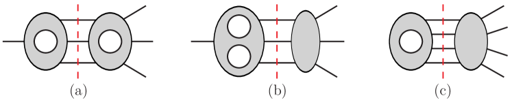
Figure 10: The three box cuts. These cuts have been evaluated in $D$ dimensions.

The method outlined above efficiently solves the problem of evaluating unitarity cuts in four dimensions in ${\cal N}=4$ sYM. However, because we are interested in computing the amplitudes in $(D>4)$-dimensions, this is not sufficient; the loop momenta are $D$-dimensional. Even if we are interested in amplitudes in four dimensions, we need to use a (supersymmetry-preserving DimRed ) form of dimensional regularization to regulate infrared singularities. If the cuts are evaluated in four dimensions, as described in the previous subsection, then terms that vanish when the loop momenta are restricted to four dimensions, but are non-vanishing in $D$ dimensions, could be missed. Indeed, amplitudes in theories with fewer supersymmetries DDimUnitarity ; DimShift , and ${\cal N}=4$ sYM amplitudes with more than four external legs TwoLoopSixPt , do contain such terms. Unfortunately, generic $D$-dimensional cuts are significantly more complicated than their four-dimensional counterparts. For continuous values of $D$, there is no helicity formalism, nor is there a useful on-shell superspace. Some of the additional complexity can avoided by working in $D$ dimensions, but with the ${{\cal N}=4}$ states organized according to the ${{\cal N}=1}$ super-Yang-Mills theory in ten dimensions BCDKS . Nevertheless, evaluating general cuts in this way at four loops is still difficult.

It is important to note that we do not need the full power of $D$-dimensional cuts to construct the amplitude, but only to identify any potential terms dropped by the four-dimensional cuts. Such terms are rare or even nonexistent for ${\cal N}=4$ sYM at low orders and low multiplicity. Specifically, for four-point amplitudes through three loops, and for the planar contributions through four loops, explicit computation has revealed GSB ; BRY ; BDDPR ; CompactThree ; BCDKS that the $D$-dimensional versions of the amplitudes are obtained simply by replacing the four-dimensional loop integration measure with the $D$-dimensional one,

$$\int{d^{4}p\over(2\pi)^{4}}\rightarrow\int{d^{D}p\over(2\pi)^{D}}\,,$$ (20)

and reinterpreting all Lorentz products of momenta as $D$-dimensional ones. Based on this evidence, we have every reason to believe that eq. (20) holds as well for the non-planar contributions at four loops. Although we have not checked all cuts in $D$ dimensions in this paper, we have performed a set of strong consistency checks to make it extremely unlikely that any $D$-dimensional contributions have been missed. Such checks include all two-particle cuts, and all generalized cuts that isolate a four-particle sub-amplitude (box cuts), as shown in fig. 10. As noted some time ago BRY ; BDDPR , for four-point amplitudes, the iterated two-particle cuts automatically give the same result in $D$ dimensions as in four dimensions. In the next section we will explain why the box cuts have the same property. Another powerful check comes from the new diagrammatic numerator identities BCJ ; BCJLoop , which hold in any dimension. They allow us to obtain many non-planar terms directly from planar ones. At four loops, the latter are known to be valid in $D$ dimensions BCDKS , at least for external gluon states. Because of these checks it is rather unlikely that any terms were dropped in extending the four-dimensional loop-momentum integrand to $D$ dimensions. Nevertheless, it would still be useful to evaluate a complete set of unitarity cuts in $D$ dimensions. As a step in this direction, the unitarity cuts have been confirmed for six-dimensional external and cut momenta FutureD6 , using the helicity formalism of Cheung and O’Connell OConnell and the on-shell superspace of Dennen, Huang and Siegel SixDimSusy .

III Constructing a compact ansatz

In the process of constructing amplitudes, it is helpful to have a toolkit that allows one to write down large classes of terms with essentially no computation. Even heuristic rules motivated by observed structures, or tools that capture only a subset of terms, can be rather useful. Typically, such rules allow one to quickly fix the structurally simplest terms in the amplitude, allowing the remaining effort to be focused on the more intricate ones. This strategy is especially potent when combined with the method of maximal cuts FiveLoop , which (as discussed below) allows a relatively small set of contributions to be considered in isolation.

For planar ${\cal N}=4$ sYM there are a set of powerful graphical tools. The oldest of these tools is the “rung insertion rule” BRY , which generates certain higher-loop contributions from lower-loop ones. More recently, the observed dual conformal properties of planar ${\cal N}=4$ sYM MagicIdentities ; BCDKS amplitudes have led to a powerful method for determining them, up to prefactors FiveLoop ; TwoLoopSixPt ; SpradlinLeadingSingThreeLoop ; Vergu that can be determined straightforwardly from cuts. Heuristic rules for determining the prefactors in the planar four-point case have been given as well FiveLoop ; KorchemskyZeros ; CachazoSkinner . Unfortunately, it is not clear how to extend the notion of dual conformal invariance to non-planar contributions. We also remark that the planar terms in the four-loop four-point amplitude were determined previously (without using dual conformal invariance) BCDKS . The non-planar contributions are much more intricate. In this section we will discuss tools that are useful for identifying both planar and (more importantly) non-planar contributions.

We begin by reviewing and extending some particularly useful cuts that can be expressed very simply, and in all generality, in terms of lower-loop expressions. We also discuss a tree-level identity that allows many multi-loop contributions to be constructed, up to potential contact terms. We will close this section by discussing the method of maximal cuts, which provides a systematic tool for constructing all terms in any amplitude, including contact terms.

III.1 Two-particle cuts

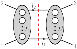
Figure 11: A two-particle cut that may be used to construct contributions to the $(L+L^{\prime}+1)$-loop amplitude from those at $L$ and $L^{\prime}$ loop orders.

A two-particle cut of a multi-loop four-point amplitude has the form shown in fig. 11 — it divides the amplitude into two lower-loop four-point amplitudes. Four-point amplitudes in ${\cal N}=4$ sYM have an especially simple dependence on the external states. This fact makes it possible to immediately write down the numerator factors for parent graphs that have two-particle cuts, in terms of lower-loop numerator factors (up to potential contact term ambiguities). This method can be applied to non-planar parent graphs as well, making it especially powerful.

This simplicity relies on the observation that all ${\cal N}=4$ sYM four-point amplitudes can be expressed in a common factorized form,

$${\cal A}_{4}^{(L)}(1,2,3,4)=g^{2L+2}{\cal K}(1,2,3,4)\,U^{(L)}(1,2,3,4)\,,$$ (21)

where ${\cal A}_{4}$ represents the full color-dressed amplitude (as distinguished from the color-stripped $A_{4}$). All of the state dependence in ${\cal A}_{4}$ is carried by the kinematic prefactor ${\cal K}=s_{12}s_{23}A_{4}^{\rm tree}$, also defined in eq. (6). All of the color dependence is carried by the state-independent universal factor $U^{(L)}$. We will use this factorization of color and state dependence to determine the terms in $U^{(L)}$ that are visible in two-particle cuts, iteratively in terms of lower-loop universal factors. This result will be valid in $D$ dimensions, whenever the lower-loop universal factors are valid in $D$ dimensions.

For four-dimensional external momenta and states, eq. (21) follows from the Ward identities for maximal supersymmetry. These identities relate all four-point amplitudes to each other at any loop order SWI ; BDDPR ; FreedmanSWI . From explicit computations, we know that this equation holds in $D$ dimensions for all states at one and two loops and at least for gluon amplitudes at three loops GSB ; BRY ; BDDPR ; GravityThree . Using the observation that, in theories with 16 supercharges, the number of states ($2^{8}$) in a massive representation of the supersymmetry algebra is the same as the number of states in a product of two short (massless) representations ($2^{4}\times 2^{4}$), Alday and Maldacena AldayMaldacena argued that the intermediate states in a $2\rightarrow 2$ scattering process form a single supermultiplet in any dimension. This argument suggests that eq. (21) also holds in any dimension, with the loop factor $U^{(L)}$ capturing the $L$-loop correction to this multi-particle intermediate state. We therefore assume that eq. (21) is valid in $D$ dimensions, for any two-particle cut of the four-loop four-point ${{\cal N}=4}$ amplitude.

In order to treat the tree-level case, $L=0$, on an equal footing with loop level, we note that the color-dressed tree amplitude in ${\cal N}=4$ sYM can be written as

$${\cal A}_{4}^{(0)}(1,2,3,4)=g^{2}A_{4}^{(0)}(1,2,3,4)\times\\ \biggl{(}\tilde{f}^{a_{4}a_{1}b}\tilde{f}^{ba_{2}a_{3}}+\tilde{f}^{a_{3}a_{1}b}\tilde{f}^{ba_{2}a_{4}}\frac{s_{23}}{s_{13}}\biggr{)}\,,$$ (22)

where $A_{4}^{(0)}\equiv A_{4}^{\rm tree}$, and we have used the color-Jacobi identity to eliminate the color factor $\tilde{f}^{a_{1}a_{2}b}\tilde{f}^{ba_{3}a_{4}}$ in favor of the other two. We also used the fact that ${\cal K}$ is crossing symmetric (see eq. (10)), which implies that all the orderings of the color-ordered tree amplitude $A_{4}^{(0)}(1,2,3,4)$ are related simply to each other, up to ratios of kinematic invariants. Dividing eq. (22) by ${\cal K}$, we see that the state-independent color-dressed universal factor at tree level, $U^{(0)}$, defined by eq. (21), is given by,

$${U}^{(0)}(1,2,3,4)=\biggl{(}\frac{\tilde{f}^{a_{4}a_{1}b}\tilde{f}^{ba_{2}a_{3}}}{s_{12}s_{23}}+\frac{\tilde{f}^{a_{3}a_{1}b}\tilde{f}^{ba_{2}a_{4}}}{s_{12}s_{13}}\biggr{)}\,.$$ (23)

In general, the universal factor $U^{(L)}$ is a sum of $L$-loop integrals. The integrands entering $U^{(L)}$ are rational functions of momentum invariants involving the loop and external momenta. Explicit formulæ for the universal factors for $L=1,2,3$, including planar and non-planar contributions, may be found by matching eq. (21) with the known amplitudes already presented in section II.1: (5), (11) and (14).

Next we evaluate the generic two-particle color-dressed cut depicted in fig. 11. It cuts the $(L+L^{\prime}+1)$-loop amplitude ${\cal A}_{4}^{(L+L^{\prime}+1)}(1,2,3,4)$ into the two four-point amplitudes ${\cal A}_{4}^{(L)}(-l_{1},1,2,l_{2})$ and ${\cal A}_{4}^{(L^{\prime})}(-l_{2},3,4,l_{1})$ of loop orders $L$ and $L^{\prime}$, respectively. The cut has the form,

$${\cal A}_{4}^{(L+L^{\prime}+1)}(1,2,3,4)\Big{|}_{\rm 2\hbox{-}cut}=i^{2}\,\sum_{{{\cal N}=4}\atop{\rm states}}{\cal A}_{4}^{(L)}(-l_{1},1,2,l_{2})\,{\cal A}_{4}^{(L^{\prime})}(-l_{2},3,4,l_{1})\,,$$ (24)

where the state sum is over the particles with momenta $l_{1}$ and $l_{2}$.

Using the factorization (21) and the state-independence of $U^{(L)}$, we can immediately rewrite the cut as follows:

$$U^{(L+L^{\prime}+1)}(1,2,3,4)\Big{|}_{\rm 2\hbox{-}cut}\times{\cal K}(1,2,3,4) = i^{2}\,U^{(L)}(-l_{1},1,2,l_{2})\,U^{(L^{\prime})}(-l_{2},3,4,l_{1})$$ (25)

$$\hskip 8.5359pt\times\sum_{{{\cal N}=4}\atop{\rm states}}{\cal K}(-l_{1},1,2,l_{2})\,{\cal K}(-l_{2},3,4,l_{1})\,.$$

Substituting in the definition of ${\cal K}$ given above, we find:

$$U^{(L+L^{\prime}+1)}(1,2,3,4)\Big{|}_{\rm 2\hbox{-}cut}\times s_{12}s_{23}A_{4}^{(0)}(1,2,3,4) = i^{2}\,U^{(L)}(-l_{1},1,2,l_{2})\,U^{(L^{\prime})}(-l_{2},3,4,l_{1})$$

$$\hskip-56.9055pt\times s_{12}^{2}\,s_{2l_{2}}s_{4l_{1}}\sum_{{{\cal N}=4}\atop{\rm states}}\,A_{4}^{(0)}(-l_{1},1,2,l_{2})\,A_{4}^{(0)}(-l_{2},3,4,l_{1})\,.$$

To evaluate this, we use the sewing relation between two four-point color-ordered ${\cal N}=4$ sYM trees BRY ; BDDPR ,

$$\sum_{{{\cal N}=4}\atop\rm states}A_{4}^{(0)}(-l_{1},1,2,l_{2})A_{4}^{(0)}(-l_{2},3,4,l_{1})=-is_{12}s_{23}\,A_{4}^{(0)}(1,2,3,4){1\over s_{2l_{2}}s_{4l_{1}}}\,.$$ (27)

This sewing relation is valid in any dimension $D$ and for any external states in the ${{\cal N}=4}$ multiplet. A straightforward way to confirm eq. (27) is to work in $D=10$ and evaluate the sum over states in components, using the fact that in $D=10$ ${\cal N}=4$ sYM is equivalent to an ${{\cal N}=1}$ theory composed of a gluon and a gluino. By dimensional reduction the sewing relation (27) then holds in any dimension $D\leq 10$. Recently, this equation has also been verified directly in six dimensions using an on-shell superspace SixDimSusy .

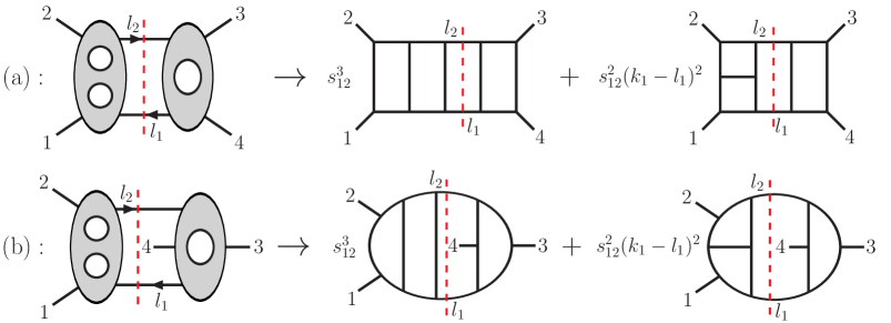
Figure 12: Sample contributions to the full color-dressed two-particle cut for $L=2$ and $L^{\prime}=1$. The diagrams on the right-hand side show some of the terms in $U^{(4)}(1,2,3,4)$ that are constructed from these cuts, using fig. 13. The explicit color factors, as well as factors of $i$, have been omitted.

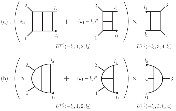
Figure 13: The lower-loop integral functions entering the cuts on the left-hand side of fig. 12. This figure displays in detail how the prefactor of the planar double-box integral appears in $U^{(2)}(-l_{1},1,2,l_{2})$ as either $s_{12}$ or $(k_{1}-l_{1})^{2}$, depending on the permutation.

Applying eq. (27) to eq. (LABEL:GenLoopTwoParticleCutRewrite2), we find the key equation for building all contributions from two-particle cuts directly in terms of the $U$s:

$$U^{(L+L^{\prime}+1)}(1,2,3,4)\Big{|}_{\rm 2\hbox{-}cut}=i\,s^{2}_{12}\,U^{(L)}(-l_{1},1,2,l_{2})\,U^{(L^{\prime})}(-l_{2},3,4,l_{1})\,.$$ (28)

Equation (28) is rather powerful. No complicated calculations remain in order to obtain all contributions visible in two-particle cuts; they are given simply by taking the product of lower-loop results. The color-dressed $U^{(L+L^{\prime}+1)}$ is given immediately as a sum over products of individual integrals residing inside the $U^{(L)}$ and $U^{(L^{\prime})}$ factors, up to terms that vanish because of the on-shell conditions, $l_{1}^{2}=l_{2}^{2}=0$. (As a straightforward exercise, one can verify that the one-loop universal factor $U^{(1)}$ — which can be extracted from eq. (5) — satisfies this equation, using the tree-level universal factor given in eq. (23).)

Figs. 12 and 13 illustrate diagrammatically some of the terms generated by eq. (28) for the case $L=2$ and $L^{\prime}=1$. For simplicity, we draw only the planar contributions of $U^{(2)}(-l_{1},1,2,l_{2})$, encoding the $\tilde{f}^{abc}$ visually in the diagrams, and we omit all factors of $i$. The denominator factors in $U^{(2)}$ and $U^{(1)}$ correspond to propagators that are visible on the left- and right-hand sides of fig. 13, respectively. Therefore they are accounted for graphically in $U^{(3)}|_{\rm 2\hbox{-}cut}$ simply by connecting the $l_{1}$ and $l_{2}$ legs of the corresponding diagrams. Similarly, the numerator factor for each parent graph on the right-hand side of fig. 12 is given by forming the product of the numerator factors for the two sewn subdiagrams in fig. 13 (taking into account the proper permutation of legs), and then multiplying by two powers of $s_{12}$.

This diagrammatic interpretation of the two-particle cuts provides a rather simple tool for generating many higher-loop contributions from known lower-loop ones. It is the mechanism behind the rung rule BRY ; BDDPR . For the planar contributions at four loops, the two-particle cuts have either $L=2$, $L^{\prime}=1$, as in fig. 12, or else $L=3$, $L^{\prime}=0$. Together, they capture diagrams (a)-(e) in fig. 5, but not diagram (f). (Diagram (f) can still be guessed from the rung rule, or constructed using a box cut, as described in the next subsection.) These cuts also do not guarantee the absence of contact terms that have no two-particle cuts, such as diagrams (f₂) and (d₂) in fig. 6. For the full four-loop amplitude described in section IV, 33 of the 50 parent graphs contain two-particle cuts (graphs 1 through 27, and graphs 40 through 45). The two-particle cuts capture the majority of the terms contributing to these graphs. Because the two-particle cut sewing algebra is valid in $D$ dimensions, all contributions obtained by iterating two-particle cuts are automatically valid in $D$ dimensions. Surprisingly, the two-particle cuts capture the majority of terms in the 33 parent graphs containing them. The fact that so many potential contact terms are absent hints at further structures to be uncovered.

We note that in ${{\cal N}=8}$ supergravity, the two-particle cuts have an equally simple structure BDDPR , which can be exploited analogously.

III.2 Box cuts

The simple structure of the four-point amplitude in ${\cal N}=4$ sYM can also be applied to (generalized) four-particle cuts that isolate a four-point sub-amplitude. A simple version of this generalization appeared already FiveLoop as a “box-substitution rule”. It allowed the construction of $L$-loop contributions with a box subgraph, starting from $(L-1)$-loop contributions with a contact interaction, as illustrated in fig. 14. Related rules were discussed in conjunction with leading singularities CachazoSkinner . Here we promote the box-substitution rule into a more general cut for ${\cal N}=4$ sYM amplitudes in $D$ dimensions, which we call the “box cut”.

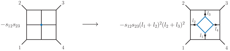
Figure 14: The box-substitution rule FiveLoop for generating a higher-loop contribution by inserting a one-loop four-point box subintegral into a four-point vertex. In this example, we substitute a box into the central four-point vertex in the four-loop “window” diagram. The result is a five-loop integral that cannot be obtained from two-particle cuts. (Note that an overall normalization factor of $s_{12}s_{23}$ has been absorbed into ${\cal K}$, relative to ref. FiveLoop .)

Consider the generalized cut of an $L$-loop $n$-point amplitude,

$${\cal A}_{n}^{(L)}\Big{|}_{\rm box~{}cut}\equiv\sum_{{{\cal N}=4}\atop\rm states}{\cal A}_{(1)}\cdots{\cal A}_{4,(i)}^{(L^{\prime})}\cdots{\cal A}_{(m)}\,,$$ (29)

that is composed of a generic set of color-dressed amplitude factors, except for the $i^{\rm th}$ such factor, which we take to be a color-dressed $L^{\prime}$-loop four-point sub-amplitude, ${\cal A}_{4,(i)}^{(L^{\prime})}$. (There may be additional cut conditions imposed on this sub-amplitude; its internal kinematics are irrelevant for the subsequent discussion.) Example of such box cuts are given in fig. 15.

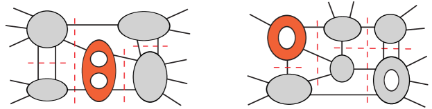
Figure 15: Two examples of multi-particle multi-loop “box cuts”. They reduce to lower-loop cuts by replacing the darker (red) four-point sub-amplitudes by four-point color-ordered trees, multiplied by known numerator and denominator factors. This property allows these cuts to be computed easily in $D$ dimensions, once the amplitudes with fewer loops are known. White holes represent loops and the darker sub-amplitudes mark four-point amplitudes amenable to reduction.

The $L^{\prime}$-loop four-point sub-amplitude of ${\cal N}=4$ sYM is special because of the factorization property (21). Labeling the cut legs by $l_{1},l_{2},l_{3},l_{4}$, we have,

$${\cal A}_{4,(i)}^{(L^{\prime})}(l_{1},l_{2},l_{3},l_{4})=A_{4,(i)}^{(0)}(l_{1},l_{2},l_{3},l_{4})\,(l_{1}+l_{2})^{2}(l_{2}+l_{3})^{2}\,U^{(L^{\prime})}(l_{1},l_{2},l_{3},l_{4})\,,$$ (30)

where, as in the previous section, we use ${\cal A}_{4}$ to represent the color-dressed amplitude, and only the color-ordered tree amplitude factor $A_{4,(i)}^{(0)}$ depends on the states crossing the cuts. Therefore we can pull the factor $U^{(L^{\prime})}$ out of the sum over states in eq. (29), leading to a simpler expression in the summand,

$${\cal A}_{n}^{(L)}\Big{|}_{\rm box~{}cut}=(l_{1}+l_{2})^{2}(l_{2}+l_{3})^{2}U^{(L^{\prime})}(l_{1},l_{2},l_{3},l_{4})\,\sum_{{{\cal N}=4}\atop\rm states}{\cal A}_{(1)}\cdots A_{4,(i)}^{(0)}\cdots{\cal A}_{(m)}\,.$$ (31)

The state-sum is identical to a lower-loop cut, that of the $(L-L^{\prime})$-loop amplitude, but utilizing the color-ordered contribution to the $i^{\rm th}$ tree. This fact immediately gives a simple relation between the $L$-loop box cut and contributions to the reduced $(L-L^{\prime})$-loop cut under the same cut conditions.

We can formally write down an equation relating the cut of an $L$-loop amplitude to a cut of a lower-loop one as,

$${\cal A}_{n}^{(L)}\Big{|}_{\rm box~{}cut}=(l_{1}+l_{2})^{2}(l_{2}+l_{3})^{2}\,U^{(L^{\prime})}(l_{1},l_{2},l_{3},l_{4})\,\tilde{{\cal A}}_{n}^{(L-L^{\prime})}\Big{|}_{\rm cut}\,.$$ (32)

We introduced the reduced cut $\tilde{{\cal A}}$ notation to emphasize that the state-sum in eq. (31) is exactly a $(L-L^{\prime})$ loop unitarity cut which is color-dressed with $\tilde{f}^{abc}$ everywhere, except for the four-point color-ordered tree amplitude whose associated color factors are accounted for in the $L^{\prime}$-loop universal factor $U^{(L^{\prime})}$.

Given a generalized cut that isolates an $L^{\prime}$-loop four-point sub-amplitude with legs $l_{1},l_{2},l_{3},l_{4}$, we can re-express the box cut as a recipe that can be applied easily to individual diagrammatic (integral) contributions:

• Split up the cut into three parts as in eq. (32): The reduced cut, $\tilde{{\cal A}}_{n}^{(L-L^{\prime})}\big{|}_{\rm cut}$, the kinematic factor $(l_{1}+l_{2})^{2}(l_{2}+l_{3})^{2}$, and the loop integrals $U^{(L^{\prime})}$ of the four-point sub-amplitude. (This latter part generalizes to $L^{\prime}$ loops the one-loop box integral of the box substitution rule.)

• Express the reduced cut of the known lower-loop amplitude in a diagrammatic form that corresponds to a covariant integral representation.

• The diagrams of the reduced cut may contain spurious propagators in the $(l_{1}+l_{2})^{2}$ or $(l_{2}+l_{3})^{2}$ channels, which upon multiplication cancel against the $(l_{1}+l_{2})^{2}(l_{2}+l_{3})^{2}$ prefactor in eq. (32). The result is always a diagram with an internal four-point contact vertex.

• To recover the integrals of the original box cut, insert the four-point integrals of $U^{(L^{\prime})}$ (e.g., the box integral for $L^{\prime}=1$) into the obtained four-point contact vertex of each diagram.

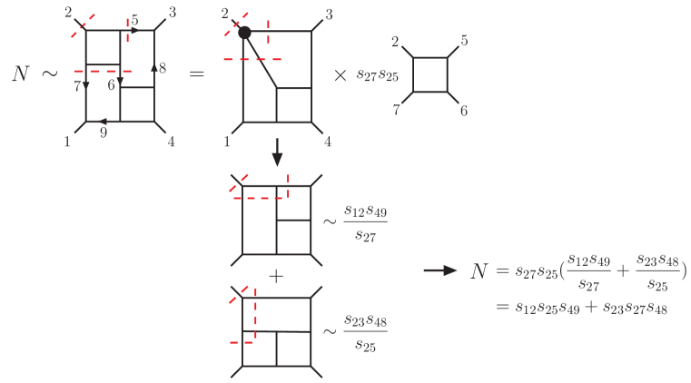
Figure 16: Application of the box cut to determine the numerator $N$ for the four-loop parent graph in fig. 5(f). The (red) dashed cut conditions around the upper left box in this diagram allow us to replace it by the product of a reduced cut diagram, some kinematical factors and a box integral. The reduced cut diagram is then expanded into two three-loop “tennis-court” diagrams, corresponding to the two allowed channels of the marked four-point vertex. The relevant kinematical pieces of the tennis-court diagrams, i.e. the numerators and the spurious propagators, are extracted from the known three-loop contribution in fig. 4(e). Assembling all the kinematical factors gives the result for $N$, which is free of spurious propagators. The result is consistent with fig. 5(f); here the numerator is symmetrized with respect to the $(1\leftrightarrow 3)$ symmetry of this parent graph.

Fig. 16 shows how the box cut can be used to determine the numerator polynomial for fig. 5(f), using the three-loop information in fig. 4(e). Although this example is planar (and is presented in a color-ordered way in the figure), it is just as simple to use the box cut for non-planar contributions. For example, inserting a box into the four-point vertex in fig. 16 in a non-planar fashion generates contributions to parent graph 29 in the full four-loop amplitude.

The box cut is an extremely efficient way to obtain contributions to parent graphs that contain a lower-loop four-point subgraph. As mentioned earlier, the $L^{\prime}=1$ box cut is closely related to the box-substitution rule. The box cut also generates contributions that are consistent with the rung rule BRY .

Box cuts capture a majority of those terms in the complete four-loop four-point amplitude in section IV that are not determined by two-particle cuts. Of the 17 parent graphs that do not have two-particle cuts, 13 of them have box cuts. The only four that have neither two-particle cuts nor box cuts are graphs 39, 48, 49 and 50. In fact, most of the parent integrals have multiple box cuts, allowing us to constrain their numerators under complementary cut conditions, and to fix many of the contact terms.

From the above covariant derivation it follows that box cuts are valid in any dimension, if both the reduced cut $A_{n}^{(L-L^{\prime})}\big{|}_{\rm cut}$ and the four-point universal factor $U^{(L^{\prime})}$ are known in $D$ dimensions. As a practical matter, the universal factors entering the lower-loop amplitudes should already be known in $D$ dimensions, prior to attempting the higher-loop calculation in $D$ dimensions. In the case relevant to this paper, $L=4$ and $n=4$, all we need as input are the $L^{\prime}=1,2,3$ four-point amplitudes, which are indeed known in $D$ dimensions BRY ; BDDPR ; GravityThree .

The effectiveness of the box cut suggests that one should investigate analogous “pentagon cuts”, etc., which isolate sub-amplitudes with five or more legs. Both the color and kinematic structure of the five- and higher-point loop amplitudes is, however, more intricate, and there is no simple factorization property similar to eq. (30). (See for example, the five- and six-point loop amplitudes described in refs. DimShift ; TwoLoopSixPt ; Vergu .)

The box cut also easily generalizes to ${{\cal N}=8}$ supergravity, because its four-point amplitude has a factorized form similar to eq. (21), which is related to the existence of analogous supersymmetric Ward identities SWI .

III.3 Color-kinematic duality

In the early 1980s, radiation zeroes appearing in certain gauge-theory cross sections were traced back to a curious identity obeyed by tree-level four-point amplitudes Zhu ; GHL . This curiousity turns out to be the simplest of a set of relations arising from a general tree-level duality between color factors and kinematic numerators BCJ . If one assumes that the duality holds for an arbitrary number of external states, one can derive BCJ new relations among color-ordered tree amplitudes, which have since been proven BoFengBCJProof . Similar relations among string theory amplitudes have also been proven recently BjerrumBohrJacobi ; StiebergerJacobi . In the low-energy limit, the string-theory relations become identical to two types of field-theory relations: the Kleiss-Kuijf relations KleissKuijf (which follow from color considerations alone DDDM ) and the amplitude relations which follow from the color-kinematic duality.

In this subsection, we discuss how the four-point tree-level color-kinematic identity may be combined with generalized unitarity at the loop level BCJ , particularly to the construction of the four-loop ${\cal N}=4$ sYM amplitude. In short, the identity relates sets of three parent graphs that only differ in how a four-point cubic tree graph is glued into the rest of the graph. Evidence that the color-kinematic duality also holds directly at the loop level, without the need to impose on-shell conditions, was presented recently for the three-loop four-point amplitude BCJLoop .

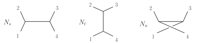
Figure 17: Graphs for the four-point tree amplitude. Contact terms are absorbed into the diagrams as inverse propagators. Each diagram is associated with a color factor obtained by dressing the vertices with an $\tilde{f}^{abc}$, as in section II.1.

Consider the color-dressed four-point tree amplitude. Just as for the loop amplitudes discussed in section II.1, it can be written as a sum of color factors $C_{i}$ multiplied by kinematic factors. The kinematic factors can be further divided into denominators, which are propagators associated with (tree-level) parent graphs, and numerators $N_{i}$. As in section II.1, contact terms can be absorbed into the $N_{i}$, so that we require only the three cubic graphs shown in fig. 17. In this representation the amplitude is,

$${\cal A}^{\rm tree}_{4}=g^{2}\biggl{(}\frac{N_{s}C_{s}}{s}+\frac{N_{t}C_{t}}{t}+\frac{N_{u}C_{u}}{u}\biggr{)}\,,$$ (33)

where $s=(k_{1}+k_{2})^{2}$, $t=(k_{2}+k_{3})^{2}$ and $u=(k_{1}+k_{3})^{2}$ correspond to the three channels, and

$$C_{s}\equiv\tilde{f}^{a_{1}a_{2}b}\tilde{f}^{ba_{3}a_{4}}\,,\hskip 28.45274ptC_{t}\equiv\tilde{f}^{a_{2}a_{3}b}\tilde{f}^{ba_{4}a_{1}}\,,\hskip 28.45274ptC_{u}\equiv\tilde{f}^{a_{4}a_{2}b}\tilde{f}^{ba_{3}a_{1}}\,,$$ (34)

are color factors corresponding to the three graphs in fig. 17. The color factors of the graphs satisfy the Jacobi identity,

$$C_{u}=C_{s}-C_{t}\,.$$ (35)

The $N_{i}$ in eq. (33) contain momentum invariants, polarization vectors, spinors and superspace Grassmann parameters. The only real restriction on them is that eq. (33) gives the correct color-dressed tree amplitude. Hence there is a tremendous amount of freedom in the definition of the numerator factors. (Non-local $N_{i}$ could even be allowed.) This freedom is just the tree-level analog of the inherent ambiguity in the multi-loop parent-graph decomposition mentioned in section II.2. We refer to the invariance of eq. (33) under this freedom as a “generalized gauge invariance.” For every such generalized gauge choice for the four-point ${\cal N}=4$ sYM amplitude, the numerator factors must satisfy the identity BCJ ,

$$N_{u}=N_{s}-N_{t}\,,$$ (36)

in concordance with the color Jacobi identity (35). We emphasize that the identity (36) is only between the numerator factors; it does not involve the propagators associated with the $s$, $t$, and $u$ channel graphs. It is fairly straightforward to check that these identities hold in $D$ dimensions by direct computation Zhu . Although it is not relevant to this section, it should be noted that for higher-point tree amplitudes the color-kinematic duality is only manifest for certain special generalized gauge choices BCJ ; Square .

In conjunction with the unitarity method, the tree-level four-point numerator identity (36) becomes quite powerful. In every multi-loop parent graph that contains four on-shell propagators arrayed around a four-point tree sub-amplitude, it relates the numerator factor to those of two other parent graphs satisfying those conditions BCJ . The three multi-loop parent graphs correspond to gluing in the four-point cubic tree graph in its $s$, $t$, or $u$ channel configuration. For every line of each cubic graph this identity will always relate the numerators of three graphs. However, the relations do not have to be manifest in a given amplitude representation, because of the freedom to move contact terms associated with other propagators between different graphs.

These relations allow one to take kinematic numerator information, obtained using dual-conformal symmetry (for planar graphs), two-particle cuts and box cuts, and export that information to other parent graphs or contributions for which such methods are not applicable.

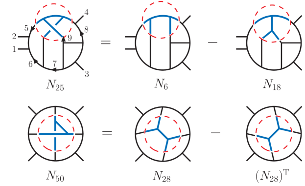
Figure 18: Two nontrivial relations between numerators of planar and non-planar contributions at four loops, which follow from the tree-level numerator relations in fig. 17. For the three graphs in each relation, the configuration of lines outside the region marked by a dashed circle is identical; the only difference is for the lines fully inside this region. The relation on the second line involves the same graph numerator $N_{28}$ with two different labelings of momenta.

To see how this works, consider the two four-loop examples illustrated in fig. 18. In each case, the numerators on the right-hand side are planar, and are relatively simple to obtain using two-particle cuts ($N_{6}$ and $N_{18}$) or box cuts ($N_{28}$, at least up to contact terms). We then use the four-point tree color-kinematic duality to obtain the bulk of the non-planar graph numerators on the left-hand side of each equation. The numerators of the four-point tree amplitudes entering the cut satisfy the relation (36) (see also fig. 17). The remaining contributions from the outside of the dashed circle are identical in all three contributions. Hence we obtain a numerator identity for the loop integrands,

$$N_{a}\bigr{|}_{\rm cut}=(N_{b}-N_{c})\bigr{|}_{\rm cut}\,,$$ (37)

where the $N_{x}$ are the kinematic numerators of the integrals corresponding to the graphs in fig. 18. This relation is valid in $D$ dimensions. However, it holds only for the numerator terms that are nonvanishing under the imposed on-shell conditions, in which the four legs crossing the dashed circle are put on shell. Also, it should be realized that some contact terms may be distributed for convenience into other graphs. That is, there are a large number of coupled equations obtained from these constraints, and it is not necessary to satisfy each one simultaneously for all contact terms.

To illustrate these ideas in more detail, consider the identity on the first row of fig. 18. It involves the numerators $N_{25},N_{6}$ and $N_{18}$ which are presented in the next section, in figs. 20, 21 and 22, and also in appendix C. We relabel the lines to match the labels in fig. 18, obtaining,

$$N^{\rm fig.\,\ref{TwistExamplesFigure}}_{25} = -s_{12}(s_{45}s_{38}-s_{12}s_{37})+l_{9}^{2}s_{12}s_{45}+l_{6}^{2}l_{8}^{2}s_{12}\,,$$

$$N^{\rm fig.\,\ref{TwistExamplesFigure}}_{6} = s^{2}_{12}s_{45}\bigr{|}_{\{3\leftrightarrow 4,5\rightarrow 7\}}=s^{2}_{12}s_{37}\,,$$

$$N^{\rm fig.\,\ref{TwistExamplesFigure}}_{18} = s_{12}s_{35}s_{46}\bigr{|}_{\{3\leftrightarrow 4,6\rightarrow 8\}}=s_{12}s_{45}s_{38}\,.$$ (38)

In addition, numerator $N^{\rm fig.\,\ref{TwistExamplesFigure}}_{25}$ picks up a sign relative to $N_{25}$ in fig. 22. That is because the deformation of graph 25 in fig. 22 into the graph in fig. 18 requires an odd number of three-vertex reorderings (three). Each reordering results in a minus sign (from the structure constants) for the color factor $C_{25}$, and a corresponding minus sign for $N_{25}$.

Using eq. (38), it is easy to see that the numerator relation (almost) holds on the cut:

$$N^{\rm fig.\,\ref{TwistExamplesFigure}}_{25}\bigr{|}_{\rm cut}=(N^{\rm fig.\,\ref{TwistExamplesFigure}}_{6}-N^{\rm fig.\,\ref{TwistExamplesFigure}}_{18})\bigr{|}_{\rm cut}\,.$$ (39)

The on-shell conditions on the legs crossing the dashed circle include $l_{9}^{2}=0$, so the term $l_{9}^{2}s_{12}s_{45}$ in eq. (38) should be set to zero. What about the term $l_{6}^{2}l_{8}^{2}s_{12}$? It is not zero on the cut, so it should be accounted for. The alert reader will notice that canceling propagators 6 and 8 in graph 25 in fig. 22 gives a graph that is topologically identical to that obtained by canceling propagators 5 and 8 (or 6 and 7) in graph 28. Also, terms containing $l_{5}^{2}l_{8}^{2}$ and $l_{6}^{2}l_{7}^{2}$ are present in $N_{28}$. These features allow the $l_{6}^{2}l_{8}^{2}s_{12}$ contact term in $N_{25}$ to be moved elsewhere to be consistent with the identity. However, the presence of overlapping identities can complicate their application, when all contact terms are retained.

The second relation in fig. 18 works similarly. The same graph 28 appears twice on the right-hand side, with two different labelings. It is worth noting that for our choice of numerators $N_{28}$ and $N_{50}$, as given in figs. 22 and 25 and appendix C, this particular relation holds even including all contact terms.

It has been conjectured recently BCJLoop that a representation exists for all multi-loop amplitudes in which all color-kinematic duality relations are manifest for all graphs, and with no internal on-shell conditions imposed. This conjecture has been confirmed for the three-loop four-point amplitude of ${\cal N}=4$ sYM, as well as for certain lower-loop cases BCJLoop , but it remains to be tested more generally. Strong evidence in favor of the conjecture would be provided if the four-loop amplitude presented here can be rearranged into such a duality-satisfying form. We leave this exercise to future work.

At four loops, the three rules just presented can be used to generate all non-contact-term contributions to the ${\cal N}=4$ sYM amplitude, as well as many of the contact-term contributions. To ensure that all contact terms are captured correctly, we turn to the method of maximal cuts.

III.4 Method of Maximal Cuts

The method of maximal cuts FiveLoop ; CompactThree offers a particularly efficient means for determining the numerator polynomials for each parent integral. In this method we start from generalized cuts with the maximum number of cut propagators (maximal cuts) and match these cuts against an initial ansatz. If an ansatz has been constructed that covers all non-contact-term contributions (for example, by using the three rules just presented), then this step is merely one of cut-verification. Next we systematically reduce the number of cut propagators (by one at each step) and match these (near-maximal) cuts — capturing in the process all potential contact contributions.

It is important that massless on-shell three-point amplitudes are non-vanishing and non-singular BCFGeneralized , for appropriate choices of complex cut loop momenta GoroffSagnotti ; WittenTopologicalString . The maximal cuts of four-point amplitudes involve products of only three-point tree amplitudes, and are the simplest cuts to evaluate. Near-maximal cuts, in which one or two of the maximal-cut propagators have been allowed to go off shell, are the next simplest to evaluate, and so on.

The advantage of the maximal-cut method is that it allows one to focus on a small number of terms at a time, namely those that become nonvanishing when a particular propagator is allowed to go off shell. This feature reduces the computational complexity at each stage, allowing us to efficiently find compact representations of amplitudes with the desired properties. We note that the “leading-singularity” technique, which is applicable to maximally supersymmetric amplitudes, is also based on cutting a maximal or near-maximal number of propagators CachazoSkinner ; CachazoLeading ; LeadingSingularityCalcs , but in addition it makes use of further conditions from hidden singularities that are special to four dimensions.

In practice the method of maximal cuts allows the sequential improvement of an ansatz for the numerator factor of each parent graph. Every new cut identifies the presence of missing pieces, which were left undetermined by the previous cuts, and which can be assigned to one of the parent graphs contributing to the cut. Because these pieces vanish on the previous set of cuts, they will contain an inverse propagator factor associated with the last propagator to be allowed to go off shell. Once new cuts cease to reveal any more missing pieces, the ansatz is generally complete and is ready for systematic cut-verification.

Although the maximal-cut method can be applied to $D$-dimensional cuts, in order to simplify their evaluation we restrict many of the cuts to have four-dimensional momenta for both internal and external lines. As we often evaluate these cuts numerically, it is useful to build an ansatz for any missing pieces, which consists of a Lorentz-covariant numerator polynomial containing unknown constant coefficients. We reduce the number of unknowns in the ansatz by assuming that no individual term in it violates the expected ultraviolet power-counting bound (eq. (41) below) BDDPR ; HoweStelleRevisited . These assumptions are, of course, validated by comparing against a spanning set of cuts after the amplitude has been constructed.

At four loops, the bound (41) predicts that at most four powers of loop momenta (or at most two inverse propagator factors $l_{n}^{2}$) can appear in any numerator polynomial. This restriction allow us to focus our attention on the maximal and near-maximal cuts that have at least 11 cut conditions, $l^{2}_{i}=0$, out of the maximal 13 (corresponding to the 13 propagators of the parent graphs). Examples of such cuts are shown in fig. 7. At the level of 11 cut conditions, there are always some quartic monomials of the form $l_{n}^{2}l_{m}^{2}$ that are non-vanishing. As one cycles through all cuts at this level, all such quartic terms will be detected, and their coefficients will be fixed. Similarly, one can show that these cuts will detect all quartic monomials of the form $p^{2}q^{2}$ and more generally $(p\cdot p^{\prime})(q\cdot q^{\prime})$, where $p,p^{\prime},q$ and $q^{\prime}$ are linear combinations of the loop momenta and external momenta. We can continue the procedure of removing on-shell conditions, one by one, until we end up with a spanning set of cuts. However, in practice, it is much simpler to stop the construction phase as soon as we suspect that the ansatz is complete.

The ansatz is then confirmed by checking that it matches the minimal spanning set of 11 cuts in fig. 8, plus the two two-particle cuts in fig. 9. We refer to this set as a spanning set because the information it provides is equivalent to that contained in all possible cuts, and minimal because any further reduction could only involve tadpole-like contributions. To show that it is a spanning set, we show that it includes all the information in the ordinary two-, three-, four- and five-particle cuts. First of all, Fig. 8(a) is just the ordinary five-particle cut. The information from the ordinary two-particle cuts is given by fig. 9(a) and (b). Ordinary four-particle cuts consist of a tree-level six-point amplitude multiplied by a one-loop six-point amplitude. We can reproduce the information in these cuts by studying those generalized cuts in which we further cut the one-loop six-point amplitude in all inequivalent ways (omitting three-point trees). This procedure leads to fig. 8(b), (c), (d) and (e). Finally, ordinary three-particle cuts leave either the product of a tree-level five-point amplitude and a two-loop five-point amplitude (with further cuts leading to fig. 8(f), (g), (h), (i), (j) and (k)), or the product of two one-loop five-point amplitudes (which does not lead to any new cut). In this classification, we can omit a cut if another cut already appears with a subset of the cut propagators.

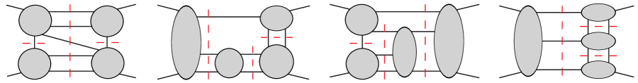
Figure 19: Four-loop examples of “MHV/$\overline{\hbox{MHV}}$-amplitude cuts”, which are composed entirely of four- and five-point tree amplitudes.

Suppose one assumes the existence of a representation of the four-loop amplitude in which each term in the numerator polynomial for each parent graph has no more than two inverse propagators, consistent with the known ${\cal N}=4$ sYM power-counting BDDPR ; HoweStelleRevisited . In this case, one only needs to check near-maximal cuts with at most two canceled propagators. Because of this, the spanning set of cuts can be restricted to products of four- and five-point tree amplitudes, as illustrated in fig. 19. (A six-point tree amplitude requires three propagators to be canceled from a maximal cut.) We refer to these as “MHV/$\overline{\hbox{MHV}}$-amplitude cuts”, because all tree amplitudes appearing in the cuts are either MHV or conjugate $\overline{\hbox{MHV}}$ amplitudes. The MHV/$\overline{\hbox{MHV}}$-amplitude cuts are useful because they are simpler to evaluate than the spanning set in figs. 8 and 9; the super-sums are particularly easy to evaluate SuperSum .

We note that when the cuts are verified using color-stripped amplitudes, in order to capture all non-planar contributions we must include cuts where the legs of each tree entering the cuts are permuted in all possible inequivalent ways.

IV The complete four-loop amplitude

We applied the construction methods outlined in the previous section to the four-loop four-point ${\cal N}=4$ sYM amplitude. The resulting amplitude is given by,

$${\cal A}_{4}^{{(4)}} = g^{10}\,{\cal K}\,\sum_{S_{4}}\,\Bigl{[}{{\textstyle\frac{1}{4}}}{\cal I}_{1}+{{\textstyle\frac{1}{4}}}{\cal I}_{2}+{{\textstyle\frac{1}{16}}}{\cal I}_{3}+{{\textstyle\frac{1}{4}}}{\cal I}_{4}+{{\textstyle\frac{1}{8}}}{\cal I}_{5}+{{\textstyle\frac{1}{2}}}{\cal I}_{6}+{{\textstyle\frac{1}{2}}}{\cal I}_{7}+{\cal I}_{8}+{{\textstyle\frac{1}{4}}}{\cal I}_{9}$$ (40)

$$+{{\textstyle\frac{1}{4}}}{\cal I}_{10}+{{\textstyle\frac{1}{2}}}{\cal I}_{11}+{{\textstyle\frac{1}{4}}}{\cal I}_{12}+{{\textstyle\frac{1}{2}}}{\cal I}_{13}+{{\textstyle\frac{1}{2}}}{\cal I}_{14}+{{\textstyle\frac{1}{4}}}{\cal I}_{15}+{\cal I}_{16}+{{\textstyle\frac{1}{2}}}{\cal I}_{17}+{\cal I}_{18}+{\cal I}_{19}$$

$$+{\cal I}_{20}+{\cal I}_{21}+{\cal I}_{22}+{\cal I}_{23}+{{\textstyle\frac{1}{2}}}{\cal I}_{24}+{\cal I}_{25}+{\cal I}_{26}+{{\textstyle\frac{1}{2}}}{\cal I}_{27}+{{\textstyle\frac{1}{4}}}{\cal I}_{28}+{\cal I}_{29}+{{\textstyle\frac{1}{2}}}{\cal I}_{30}$$

$$+{{\textstyle\frac{1}{2}}}{\cal I}_{31}+{\cal I}_{32}+{\cal I}_{33}+{{\textstyle\frac{1}{2}}}{\cal I}_{34}+{\cal I}_{35}+{\cal I}_{36}+{{\textstyle\frac{1}{2}}}{\cal I}_{37}+{{\textstyle\frac{1}{4}}}{\cal I}_{38}+{{\textstyle\frac{1}{2}}}{\cal I}_{39}+{{\textstyle\frac{1}{4}}}{\cal I}_{40}$$

$$+{{\textstyle\frac{1}{2}}}{\cal I}_{41}+{\cal I}_{42}+{\cal I}_{43}+{{\textstyle\frac{1}{2}}}{\cal I}_{44}+{{\textstyle\frac{1}{4}}}{\cal I}_{45}+{{\textstyle\frac{1}{2}}}{\cal I}_{46}+{{\textstyle\frac{1}{8}}}{\cal I}_{47}+{{\textstyle\frac{1}{2}}}{\cal I}_{48}+{{\textstyle\frac{1}{2}}}{\cal I}_{49}+{{\textstyle\frac{1}{8}}}{\cal I}_{50}\Bigr{]}\,,\hskip 8.5359pt$$

where the prefactor ${\cal K}$, defined in eq. (6), encodes the full external-state dependence, and ${\cal I}_{i}=C_{i}I_{i}$ are the color-dressed four-loop integrals. The $C_{i}$ are color factors obtained by dressing the parent graphs with structure constants $\tilde{f}^{abc}$, and are given explicitly in appendix B. The $I_{i}(s_{12},s_{23})$ are $D$-dimensional loop integrals, defined in terms of numerator factors $N_{i}$ in eq. (4), and corresponding to the 50 four-loop cubic parent graphs in figs. 20-25. The 50^th graph, which appears in eq. (40) and in fig. 25, is needed to match all cuts; however, it integrates to zero, and its associated color factor $C_{50}$ also vanishes. Thus its contribution to the integrated color-dressed amplitude is doubly vanishing. (Another reason we list this ${\cal N}=4$ sYM contribution is because it gives a nonvanishing input into the construction of the corresponding ${{\cal N}=8}$ supergravity amplitude GravityFour .)

As in the lower-loop amplitudes in section II.1, the sum runs over the 24 independent permutations of legs $\{1,2,3,4\}$, denoted by $S_{4}$, which act on both kinematic and color labels. The numerical coefficients in front of the integrals in eq. (40) are symmetry factors $1/S$, where $S$ is the number of elements in the discrete automorphism group of the corresponding unlabeled graph. As before, these factors compensate for overcounting.

As mentioned in section III, the parent graphs containing two-particle cuts, namely graphs 1–27 and 40–45, are the simplest to obtain; the bulk of the terms in their numerator polynomials are constructed using eq. (28). The remaining terms in these graphs, and all of the terms in the remaining 17 parent graphs, are obtained using box cuts (eq. (32)), plus the color-kinematic duality relation (37), as well as an evaluation of the near-maximal cuts. The amplitude’s construction was followed by a confirmation of the complete set of cuts in figs. 8 and 9.

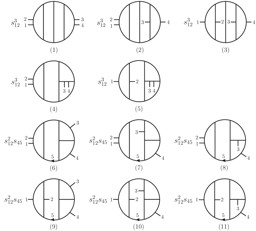
Figure 20: Integrals (1)-(11) appearing in the four-loop amplitude. The graphs encode denominator factors as the Lorentz square of the momenta flowing across every internal line, and color factors following the rules defined in fig. 1. The momentum-dependent factor in front of each graph represents the numerator factor $N_{i}$ that resides inside the integral $I_{i}$, where $(i)$ is the label below each graph. Numbers $1,2,3,4$ label the external (outgoing) momenta. The internal legs carry momenta as signified by the arrows (here only leg 5 is labeled). The kinematic variables are defined as $s_{ij}=s_{i,j}=(l_{i}+l_{j})^{2}$ and in the following figures $s_{i,\overline{j}}=(l_{i}-l_{j})^{2}$ and $\tau_{ij}=2l_{i}\cdot l_{j}$, where $l_{i}$ is the momentum of leg $i$. A specific (clockwise) orientation of each cubic vertex (in the plane of the figure) is implied here. Due to the antisymmetry of the structure constants, any noncyclic reordering of a vertex should be accompanied by a sign flip of the numerator factor.

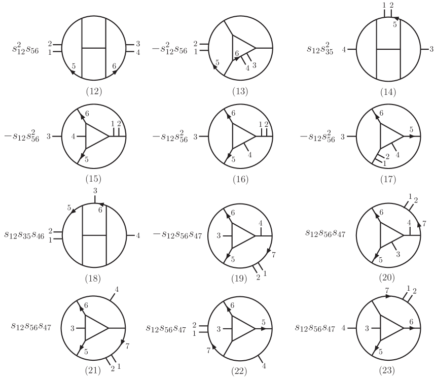
Figure 21: Integrals (12)-(23) appearing in the four-loop amplitude. The notation follows that of fig. 20.

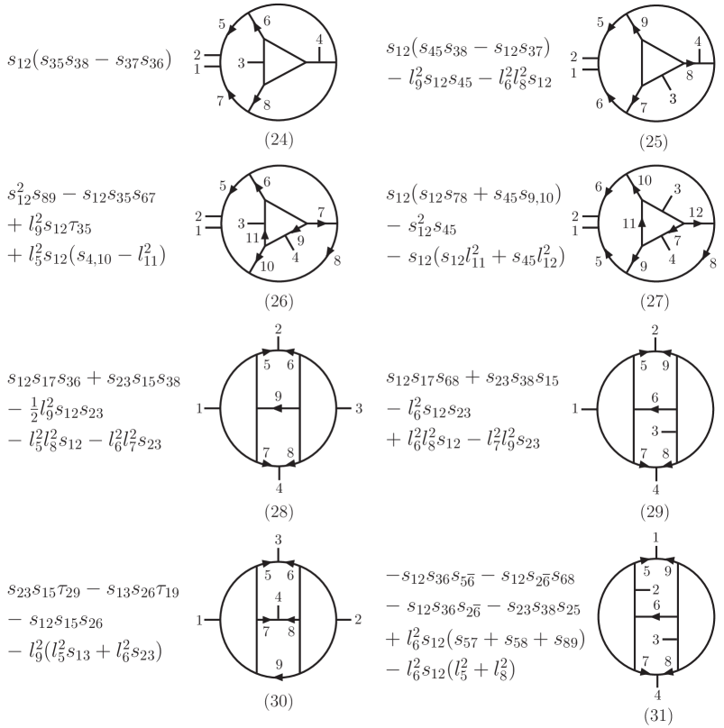
Figure 22: Integrals (24)-(31) appearing in the four-loop amplitude. The notation follows that of fig. 20.

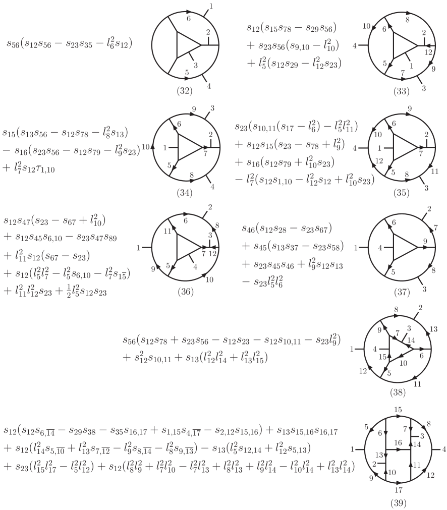
Figure 23: Integrals (32)-(39) appearing in the four-loop amplitude. The notation follows that of fig. 20.

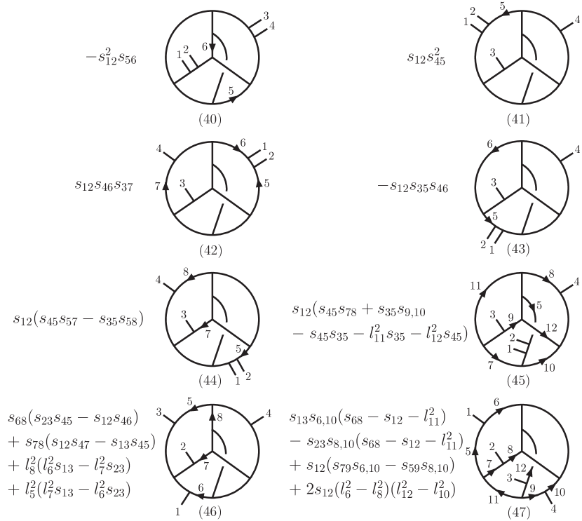
Figure 24: Integrals (40)-(47) appearing in the four-loop amplitude. The notation follows that of fig. 20.

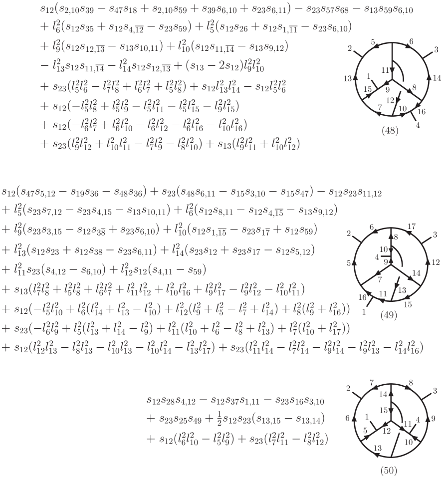
Figure 25: Integrals (48)-(49) appearing in the four-loop amplitude. Integral (50) is required for the ansatz to match the color-stripped cut at the level of the integrand. However, it does not contribute to the color-dressed amplitude. The notation follows that of fig. 20.

V Ultraviolet properties in higher dimensions

In this section we examine the UV behavior of the four-point ${\cal N}=4$ sYM amplitude in its critical dimension, i.e., the lowest dimension in which it diverges. This issue is of some importance because it provides a simpler venue than ${{\cal N}=8}$ supergravity for studying UV cancellations in theories with maximal supersymmetry. For ${\cal N}=4$ sYM, an analysis of supersymmetric cancellations in two-particle cuts (and more generally, in ordinary $m$-particle cuts that have only MHV amplitudes on either side of the cut), suggested the UV finiteness bound BDDPR ,

$$D<D_{c}=4+\frac{6}{L}\hskip 28.45274pt(L>1)\,.$$ (41)

One-loop amplitudes, corresponding to $L=1$, are special as they are UV finite for $D<8$, not $D<10$. The bound (41) is somewhat stronger than earlier superspace power counting bounds HoweStelleYangMills , although all bounds agree that the theory is UV finite in $D=4$. The bound (41) is consistent with a formulation of the theory having $3/4$ of the supercharges manifestly realized, and it has been confirmed HoweStelleRevisited using ${\cal N}=\nobreak 3$ harmonic superspace HarmonicSuperspace . Explicit computations (including the ones discussed in this paper) demonstrate that this bound is saturated through at least four loops BRY ; BDDPR ; ABDK ; Finite . It is straightforward to verify from the planar amplitude in ref. FiveLoop that the same result holds in the large-$N_{c}$ limit at five loops.

An interesting question concerns the UV behavior of the different color terms. For an $SU(N_{c})$ gauge group it is convenient to expand the amplitude in the trace basis — i.e. traces of products of generators in the fundamental representation, as in eq. (1), but including also terms that are subleading in the $1/N_{c}$ expansion. For a four-particle amplitude there are only single- and double-trace terms. This decomposition follows quite closely that of the terms in the effective action that have four or fewer field strength tensors. The single-trace terms satisfy the finiteness bound (41). As noted already in refs. DurhamAndCopenhagenTalks , double-trace terms at three and four loops exhibit additional cancellations which increase their critical dimension. These cancellations have been discussed in refs. DoubleTraceBerkovits ; BG2010 , which suggest double-trace terms should instead satisfy the finiteness bound,

$$D<4+\frac{8}{L}\hskip 28.45274pt(L>2)\,.$$ (42)

This formula is equivalent to the statement that an additional momentum invariant ($s$, $t$ or $u$) can be extracted from the double-trace terms than the single-trace terms, at each loop order. As a statement about counterterms, it implies that the leading double-trace counterterms for $L>2$ would have four covariant derivatives, for example $\,{\rm Tr}({\cal D}^{4}F^{2})\,{\rm Tr}(F^{2})$, in contrast to the two derivatives characteristic of the single-trace counterterms $\,{\rm Tr}({\cal D}^{2}F^{4})$. In a superspace description, the dimension of the double-trace counterterms would then be consistent, curiously, with the existence of a superspace formalism for these terms that preserves manifestly all sixteen supercharges.

Here we provide details of the cancellations observed in refs. DurhamAndCopenhagenTalks and affirm the double-trace power-count bound (42) for three and four loops. Moreover, by direct integration of the results we show that at three loops the double-trace bound is saturated. At four loops, we have not evaluated the required integrals in $D=6$, so it is possible (though perhaps unlikely) that the behavior of the double-trace terms is better than this bound.

V.1 One-loop ultraviolet divergence

Before turning to the four-loop amplitude, it is useful to review and expand on the lower-loop results. Let us consider first the color-dressed one-loop amplitude in eq. (5). For each of the contributing integrals it is necessary to specify the corresponding color factor. The trace basis, in which the color factors are expressed in terms of traces of products of group generators $T^{a_{i}}$ in the fundamental representation, is convenient for discussing the UV divergences for an $SU(N_{c})$ gauge group. The basis elements are:

$$\,{\rm Tr}_{ijkl}\ \equiv\ \,{\rm Tr}(T^{a_{i}}T^{a_{j}}T^{a_{k}}T^{a_{l}}),\qquad\,{\rm Tr}_{ij}\ \equiv\ \,{\rm Tr}(T^{a_{i}}T^{a_{j}})=\delta^{a_{i}a_{j}}\,.$$ (43)

(In general one may also add to the basis $\,{\rm Tr}(T^{a_{i}})$, $\,{\rm Tr}(T^{a_{i}}T^{a_{j}}T^{a_{k}})$, etc.  For four-point amplitudes the traces of length one and three must appear together; for $SU(N_{c})$ they are not necessary, because $\,{\rm Tr}(T^{a})=0$.)

The color factor of the box integral, given in eq. (7), may be expressed in the trace basis as

$$C^{\rm Box}_{1234}=N_{c}\,(\,{\rm Tr}_{1234}+\,{\rm Tr}_{1432})+2\,(\,{\rm Tr}_{12}\,{\rm Tr}_{34}+\,{\rm Tr}_{14}\,{\rm Tr}_{23}+\,{\rm Tr}_{13}\,{\rm Tr}_{24})\,.$$ (44)

The lowest dimension in which the one-loop box integral in eq. (8) develops an ultraviolet divergence is $D=8$. Near $D=8$, we have

$$I^{{\rm box},\,D=8-2\epsilon}(s_{12},s_{23})\Bigr{|}_{\rm pole}={1\over 6\,(4\pi)^{4}\,\epsilon}\,.$$ (45)

From eqs. (5) and (44) it then follows that the divergence of the one-loop amplitude in the critical dimension is given by

$${\cal A}_{4}^{{(1)}}(1,2,3,4)\Bigr{|}^{SU(N_{c})}_{\rm pole} = -{g^{4}\,{\cal K}\over 6\,(4\pi)^{4}\,\epsilon}\Bigl{(}N_{c}\,(\,{\rm Tr}_{1324}+\,{\rm Tr}_{1423}+\,{\rm Tr}_{1243}+\,{\rm Tr}_{1342}+\,{\rm Tr}_{1234}+\,{\rm Tr}_{1432})$$ (46)

$$\hskip 51.21504pt\hbox{}+6\,(\,{\rm Tr}_{12}\,{\rm Tr}_{34}+\,{\rm Tr}_{14}\,{\rm Tr}_{23}+\,{\rm Tr}_{13}\,{\rm Tr}_{24})\Bigr{)}\,.$$

At this loop order, the coefficients of the double-trace terms, relative to the single-trace ones, are fixed by a $U(1)$ decoupling identity, or dual Ward identity BKColor .

For a general gauge group $G$ the UV divergence is expressed in terms of three independent color tensors: the two tree-level tensors and the irreducible one-loop tensor $C^{\rm Box}_{1234}$ in eq. (7):

$${\cal A}_{4}^{{(1)}}(1,2,3,4)\Bigr{|}^{G}_{\rm pole}=-{g^{4}\,{\cal K}\over 6\,(4\pi)^{4}\,\epsilon}\Bigl{(}-\frac{1}{2}C_{A}(\tilde{f}^{a_{1}a_{2}b}\tilde{f}^{ba_{3}a_{4}}+\tilde{f}^{a_{2}a_{3}b}\tilde{f}^{ba_{4}a_{1}})+3C^{\rm Box}_{1234}\Bigr{)}\,,$$ (47)

where $C_{A}$ is the quadratic Casimir in the adjoint representation, normalized as in eq. (129) of appendix B. Note that the Bose symmetry of the divergence is not manifest in this form. As discussed in appendix B, any one-loop four-point quantity can be expressed in terms of these three color tensors. Thus at one loop, in the critical dimension $D_{c}=8$, the coefficients of all listed color structures diverge and there are no additional hidden cancellations.

V.2 Two-loop ultraviolet divergence

A similar analysis may be carried out for the two-loop four-point ${\cal N}=4$ sYM amplitude, which is given in eq. (11) in terms of planar and non-planar double-box integrals $I^{{\rm(P)}}$ and $I^{{\rm(NP)}}$. These integrals first diverge in $D=7$ and their poles in $D=7-2\epsilon$ are BDDPR ,

$$V^{{\rm(P)}} \equiv {I^{{\rm(P)},\,D=7-2\epsilon}\bigr{|}_{\rm pole}\over s_{12}}=-{\pi\over 20\,(4\pi)^{7}\,\epsilon}\,,$$ (48)

$$V^{{\rm(NP)}} \equiv {I^{{\rm(NP)},\,D=7-2\epsilon}\bigr{|}_{\rm pole}\over s_{12}}=-{\pi\over 30\,(4\pi)^{7}\,\epsilon}\,.$$ (49)

For an $SU(N_{c})$ gauge group, the planar and non-planar two-loop color tensors $C^{{\rm(P)}}_{1234}$ and $C^{{\rm(NP)}}_{1234}$ defined in eq. (13) become, in the trace basis,

$$C^{{\rm(P)}}_{1234} = (N_{c}^{2}+2)\,(\,{\rm Tr}_{1234}+\,{\rm Tr}_{1432})+2\,(\,{\rm Tr}_{1243}+\,{\rm Tr}_{1342})-4\,(\,{\rm Tr}_{1423}+\,{\rm Tr}_{1324})$$ (50)

$$\hskip 0.0pt\hbox{}+6N_{c}\,{\rm Tr}_{12}\,{\rm Tr}_{34}\,,$$

$$C^{{\rm(NP)}}_{1234} = 2\,(\,{\rm Tr}_{1234}+\,{\rm Tr}_{1432})+2\,(\,{\rm Tr}_{1243}+\,{\rm Tr}_{1342})-4\,(\,{\rm Tr}_{1423}+\,{\rm Tr}_{1324})$$ (51)

$$\hskip 0.0pt\hbox{}+2N_{c}{}\,(2\,{\rm Tr}_{12}\,{\rm Tr}_{34}-\,{\rm Tr}_{13}\,{\rm Tr}_{24}-\,{\rm Tr}_{14}\,{\rm Tr}_{23})\,.$$

The full amplitude was originally presented in the trace basis BRY . In terms of $V^{{\rm(P)}}$ and $V^{{\rm(NP)}}$, the UV divergence of the amplitude (11) is,

$${\cal A}_{4}^{{(2)}}(1,2,3,4)\Bigr{|}^{SU(N_{c})}_{\rm pole} = -\,g^{6}\,{\cal K}\,\biggl{[}\Bigl{(}N_{c}^{2}\,V^{{\rm(P)}}+12(V^{{\rm(P)}}+V^{{\rm(NP)}})\Bigr{)}$$

$$\hskip-42.67912pt\hbox{}\times\Bigl{(}s_{12}\,(\,{\rm Tr}_{1324}+\,{\rm Tr}_{1423})+s_{23}\,(\,{\rm Tr}_{1243}+\,{\rm Tr}_{1342})+s_{13}\,(\,{\rm Tr}_{1234}+\,{\rm Tr}_{1432})\Bigr{)}$$

$$\hskip-42.67912pt\hbox{}-12\,N_{c}\,(V^{{\rm(P)}}+V^{{\rm(NP)}})\Bigl{(}s_{12}\,{\rm Tr}_{12}\,{\rm Tr}_{34}+s_{23}\,{\rm Tr}_{14}\,{\rm Tr}_{23}+s_{13}\,{\rm Tr}_{13}\,{\rm Tr}_{24}\Bigr{)}\biggr{]}\,.$$

Inserting the planar and non-planar integral poles (48) and (49) into eq. (V.2), the UV divergence becomes,

$${\cal A}_{4}^{{(2)}}(1,2,3,4)\Bigr{|}^{SU(N_{c})}_{\rm pole} = {g^{6}\,\pi\,{\cal K}\over 20\,(4\pi)^{7}\,\epsilon}\Bigl{[}(N_{c}^{2}+20)\Bigl{(}s_{12}\,(\,{\rm Tr}_{1324}+\,{\rm Tr}_{1423})$$

$$\hskip 99.58464pt\hbox{}+s_{23}\,(\,{\rm Tr}_{1243}+\,{\rm Tr}_{1342})+s_{13}\,(\,{\rm Tr}_{1234}+\,{\rm Tr}_{1432})\Bigr{)}$$

$$\hskip 56.9055pt\hbox{}-20N_{c}\,\Bigl{(}s_{12}\,{\rm Tr}_{12}\,{\rm Tr}_{34}+s_{23}\,{\rm Tr}_{14}\,{\rm Tr}_{23}+s_{13}\,{\rm Tr}_{13}\,{\rm Tr}_{24}\Bigr{)}\Bigr{]}\,.$$

As was the case at one loop, $U(1)$ decoupling identities at two loops BDFD relate the coefficients of the single- and double-trace structures. These identities provide an a priori justification that the double-trace terms diverge whenever the single-trace terms diverge, at this loop order. In slightly more detail, the double-trace coefficient is equal to the negative of a subleading-color ($N_{c}^{0}$) single-trace coefficient, plus the sum of all three leading-color ($N_{c}^{2}$) single-trace coefficients. (See eqs. (4.48)–(4.50) of ref. BDFD .) However, in the case of eq. (V.2), the relevant leading-color sum vanishes by the identity $s_{12}+s_{23}+s_{13}=0$. Thus group theory enforces the equality of the two “20”s appearing in eq. (V.2).

We may also analyze the color structure for a general gauge group $G$. In this case, the UV divergence of the two-loop amplitude depends on five independent color tensors, which we take to be the tree-level and one-loop tensors that already appear in the one-loop divergence (47), plus two new independent (irreducible) two-loop tensors. We take the latter to be two independent permutations of the tensor $C^{{\rm(P)}}_{1234}$. (All other tensors are related to these by repeated application of the Jacobi identity.) In terms of the pole parts (48) and (49) of the planar and non-planar double-box integrals, the two-loop divergence is:

$${\cal A}_{4}^{{(2)}}(1,2,3,4)\Bigr{|}^{G}_{\rm pole} = g^{6}\,{\cal K}\biggl{[}\frac{1}{4}C_{A}^{2}V^{{\rm(P)}}(s_{12}\tilde{f}^{a_{2}a_{3}b}\tilde{f}^{ba_{4}a_{1}}+s_{23}\tilde{f}^{a_{1}a_{2}b}\tilde{f}^{ba_{3}a_{4}})$$

$$\hbox{}\hskip-11.38092pt+(V^{{\rm(P)}}+V^{{\rm(NP)}})(3C_{A}C^{\rm Box}_{1234}s_{13}+2C^{{\rm(P)}}_{1234}(s_{12}-s_{13})+2C^{{\rm(P)}}_{2341}(s_{23}-s_{13}))\biggr{]}.$$

The five color tensors appearing in eq. (V.2) form a basis in the space of two-loop four-point color tensors (see appendix B). Each of their coefficients diverges in the critical dimension $D_{c}=7$, and we see no natural combination of coefficients for which the $D=7$ divergence cancels.

V.3 Three-loop ultraviolet divergence

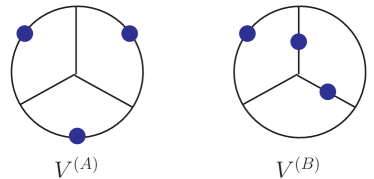
Figure 26: The vacuum-like graphs describing the three-loop UV divergences in $D=6$. The large (blue) dots indicate that a propagator appears squared, or doubled.

Let us proceed with a similar discussion of the UV divergences of the three-loop four-point amplitude given in eq. (14) and fig. 4. In this case the critical dimension is $D_{c}=6$. In the representation of the three-loop amplitude given in fig. 4, integrals (a)-(d) and (h) are all finite in the critical dimension. Only integrals (e), (f), (g) and (i) contribute to the UV divergence, because they have numerator polynomials that are quadratic in the loop momentum. To extract the divergence we follow the procedure discussed in refs. Vladimirov ; MarcusSagnotti ; CompactThree ; GravityFour , i.e. we expand in small external momenta and keep only the leading terms. In this limit, the contributing integrals reduce to,

$$I^{\rm(e)}\rightarrow s_{12}\,V^{{\rm(A)}}\,,\hskip 11.38092ptI^{\rm(f)}\rightarrow s_{12}\,V^{{\rm(B)}}\,,\hskip 11.38092ptI^{\rm(g)}\rightarrow s_{12}\,V^{{\rm(B)}}\,,\hskip 11.38092pt$$

$$I^{\rm(i)}\rightarrow(s_{12}-s_{23})\Bigl{(}V^{{\rm(B)}}-{1\over 3}V^{{\rm(A)}}\Bigr{)}\,,$$ (55)

where $V^{{\rm(A)}}$ and $V^{{\rm(B)}}$ are the vacuum-like graphs in fig. 26. These integrals are both UV and infrared divergent. As discussed in ref. CompactThree , to extract the UV divergence we inject off-shell momenta at two vertices, thus removing the infrared divergence. The values of their UV divergences are:

$$V^{{\rm(A)}}\Bigr{|}_{\rm pole} = -\frac{1}{6\,(4\pi)^{9}\,\epsilon}\,,$$ (56)

$$V^{{\rm(B)}}\Bigr{|}_{\rm pole} = -\frac{1}{6\,(4\pi)^{9}\,\epsilon}\biggl{(}\zeta_{3}-{1\over 3}\biggr{)}\,.$$ (57)

The relevant three-loop color factors $C^{\rm(e)},\,C^{\rm(f)},\,C^{\rm(g)}$ and $C^{\rm(i)}$ are easy to express in the trace basis,

$$C^{\rm(e)} = N_{c}^{3}\,(\,{\rm Tr}_{1234}+\,{\rm Tr}_{1432})+2N_{c}^{2}\,{\rm Tr}_{12}\,{\rm Tr}_{34}$$ (58)

$$\hbox{}\hskip 0.0pt+2N_{c}\,(4\,(\,{\rm Tr}_{1234}+\,{\rm Tr}_{1432})-2\,(\,{\rm Tr}_{1243}+\,{\rm Tr}_{1342})-3\,(\,{\rm Tr}_{1423}+\,{\rm Tr}_{1324}))$$

$$\hbox{}\hskip 0.0pt-4\,(\,{\rm Tr}_{12}\,{\rm Tr}_{34}+\,{\rm Tr}_{14}\,{\rm Tr}_{23}+\,{\rm Tr}_{13}\,{\rm Tr}_{24})\,,$$

$$C^{\rm(f)} = -2N_{c}^{2}\,(\,{\rm Tr}_{14}\,{\rm Tr}_{23}+\,{\rm Tr}_{13}\,{\rm Tr}_{24})$$ (59)

$$\hbox{}\hskip 0.0pt+2N_{c}\,(4\,(\,{\rm Tr}_{1234}+\,{\rm Tr}_{1432})-2\,(\,{\rm Tr}_{1243}+\,{\rm Tr}_{1342})-3\,(\,{\rm Tr}_{1423}+\,{\rm Tr}_{1324}))$$

$$\hbox{}\hskip 0.0pt-4\,(\,{\rm Tr}_{12}\,{\rm Tr}_{34}+\,{\rm Tr}_{14}\,{\rm Tr}_{23}+\,{\rm Tr}_{13}\,{\rm Tr}_{24})\,,$$

$$C^{\rm(g)} = -4N_{c}^{2}\,{\rm Tr}_{12}\,{\rm Tr}_{34}$$ (60)

$$\hbox{}\hskip 0.0pt+2N_{c}\,(3\,(\,{\rm Tr}_{1234}+\,{\rm Tr}_{1432})-3\,(\,{\rm Tr}_{1243}+\,{\rm Tr}_{1342})-\,{\rm Tr}_{1423}-\,{\rm Tr}_{1324})\hskip 17.07182pt$$

$$\hbox{}\hskip 0.0pt-4\,(\,{\rm Tr}_{12}\,{\rm Tr}_{34}+\,{\rm Tr}_{14}\,{\rm Tr}_{23}+\,{\rm Tr}_{13}\,{\rm Tr}_{24})\,,$$

$$C^{\rm(i)} = 2N_{c}^{2}(\,{\rm Tr}_{12}\,{\rm Tr}_{34}-\,{\rm Tr}_{14}\,{\rm Tr}_{23})$$ (61)

$$\hbox{}\hskip 0.0pt+2N_{c}\,(\,{\rm Tr}_{1243}+\,{\rm Tr}_{1342}-\,{\rm Tr}_{1423}-\,{\rm Tr}_{1324})\,.$$

Using these expressions, as well as the relation (55) between the leading poles of the integrals $I^{\rm(e)},\,I^{\rm(f)},\,I^{\rm(g)},\,$ and $I^{\rm(i)}$ and the vacuum integrals $V^{{\rm(A)}}$ and $V^{{\rm(B)}}$, we find that the leading UV divergence of the three-loop amplitude in dimension $D=6-2\epsilon$ is

$${\cal A}_{4}^{{(3)}}(1,2,3,4)\Bigr{|}^{SU(N_{c})}_{\rm pole} = 2\,g^{8}\,{\cal K}\,\Bigl{(}N_{c}^{3}\,V^{{\rm(A)}}+12\,N_{c}\,(V^{{\rm(A)}}+3\,V^{{\rm(B)}})\Bigr{)}$$

$$\hskip-34.14322pt\hbox{}\times\Bigl{(}s_{12}\,(\,{\rm Tr}_{1324}+\,{\rm Tr}_{1423})+s_{23}\,(\,{\rm Tr}_{1243}+\,{\rm Tr}_{1342})+s_{13}\,(\,{\rm Tr}_{1234}+\,{\rm Tr}_{1432})\Bigr{)}\,.$$

Inserting the UV pole parts (56) and (57) of $V^{{\rm(A)}}$ and $V^{{\rm(B)}}$ then gives,

$${\cal A}_{4}^{{(3)}}(1,2,3,4)\Bigr{|}^{SU(N_{c})}_{\rm pole} = -{g^{8}\,{\cal K}\over 3\,(4\pi)^{9}\,\epsilon}(N_{c}^{3}+36\,\zeta(3)\,N_{c})$$

$$\hskip-34.14322pt\hbox{}\times\Bigl{(}s_{12}\,(\,{\rm Tr}_{1324}+\,{\rm Tr}_{1423})+s_{23}\,(\,{\rm Tr}_{1243}+\,{\rm Tr}_{1342})+s_{13}\,(\,{\rm Tr}_{1234}+\,{\rm Tr}_{1432})\Bigr{)}\,.$$

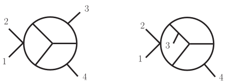
Figure 27: The leading contributions with numerators quadratic in loop momentum in fig. 4 can be absorbed into the two contact diagrams displayed here, up to relabeling of external legs. Further rearrangements push the leading terms into the diagrams of fig. 28

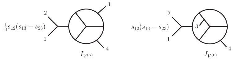
Figure 28: At three loops the leading divergence can be rearranged so that it comes from parent graphs which are one-particle reducible, depicted here in the $s_{12}$ channel. The color factors of these graphs have no double-trace contributions. The complete contribution comes from summing over all 24 permutations of external legs and multiplication by a symmetry factor of $1/4$ to remove double counts in both graphs.

A remarkable feature of the three-loop UV divergence (V.3) in the critical dimension is the absence of double-trace terms. From eqs. (58)-(61) it is clear that such terms exist separately for each integral and cancel only in the complete amplitude. This cancellation was first noted DurhamAndCopenhagenTalks as a consequence of the calculation described in this paper. Two rather different discussions of this property have been presented recently. One approach is based on the pure-spinor formalism, both in string theory in the low-energy limit DoubleTraceBerkovits and more recently in field theory BG2010 . The other approach is based on algebraic non-renormalization theorems DoubleTraceNonrenormalization , following up on earlier work BHS .

Motivated by these results, especially the structure of the leading contributions in the string theory analysis of ref. DoubleTraceBerkovits , we rearrange the leading terms in the small-momentum expansion of the integrals in fig. 4 such that double-trace terms are manifestly absent. This representation is found by noting that all terms quadratic in loop momentum, can be placed into contact-term diagrams, of the form in fig. 27. This fact suggests that the leading terms can be absorbed into the graphs with external propagators displayed in fig. 28, if we include a factor of $s_{12}$ to cancel the external propagator. After dressing the graphs with color, and a factor of $(s_{13}-s_{23})$ so that the graphs have the proper antisymmetry, it is not difficult to verify that with the numerical coefficients in fig. 28, the expression

$${\cal A}_{4}^{{(3)}}(1,2,3,4) = {1\over 4}\,g^{8}\,{\cal K}\sum_{S_{4}}\Bigl{[}C^{V^{{\rm(A)}}}_{1234}I_{V^{{\rm(A)}}}+C^{V^{{\rm(B)}}}_{1234}I_{V^{{\rm(B)}}}\Bigr{]}\;+\;\hbox{subleading},$$ (64)

has the proper leading behavior. Here $I_{V^{{\rm(A)}}}$, $I_{V^{{\rm(B)}}}$ and $C^{V^{{{\rm(A)}}}}_{1234}$, $C^{V^{{{\rm(B)}}}}_{1234}$ correspond to the integrals and color factors indicated by the graphs in fig. 28. The dropped subleading terms are better behaved in the ultraviolet than the displayed leading terms and are not relevant for our discussion. The integrals in eq. (64) are essentially just the two vacuum graphs $V^{{\rm(A)}}$ and $V^{{\rm(B)}}$, promoted to one-particle-reducible four-point integrals, and dressed with appropriate numerator factors. The color factors $C^{V^{{{\rm(A)}}}}_{1234}$ and $C^{V^{{{\rm(B)}}}}_{1234}$ are given by

$$C^{V^{{\rm(A)}}}_{1234} = \tilde{f}^{a_{1}a_{2}a_{5}}\tilde{f}^{a_{5}a_{6}a_{7}}\tilde{f}^{a_{6}a_{10}a_{8}}\tilde{f}^{a_{8}a_{11}a_{9}}\tilde{f}^{a_{9}a_{12}a_{7}}\tilde{f}^{a_{3}a_{13}a_{10}}\tilde{f}^{a_{13}a_{14}a_{11}}\tilde{f}^{a_{4}a_{12}a_{14}}$$

$$= N_{c}(N_{c}^{2}+12)\Bigl{(}\,{\rm Tr}_{1234}+\,{\rm Tr}_{1432}-\,{\rm Tr}_{1243}-\,{\rm Tr}_{1342}\Bigr{)}\,,$$

$$C^{V^{{\rm(B)}}}_{1234} = \tilde{f}^{a_{1}a_{2}a_{5}}\tilde{f}^{a_{5}a_{6}a_{7}}\tilde{f}^{a_{6}a_{13}a_{10}}\tilde{f}^{a_{3}a_{10}a_{8}}\tilde{f}^{a_{8}a_{11}a_{9}}\tilde{f}^{a_{13}a_{14}a_{11}}\tilde{f}^{a_{7}a_{9}a_{12}}\tilde{f}^{a_{4}a_{12}a_{14}}$$ (65)

$$= 12N_{c}\Bigl{(}\,{\rm Tr}_{1234}+\,{\rm Tr}_{1432}-\,{\rm Tr}_{1243}-\,{\rm Tr}_{1342}\Bigr{)}\,,$$

exposing the manifest absence of double-trace terms in the leading divergence. Because the color factors are one-particle reducible, they are proportional to the tree-level color factors; they are given by

$$C^{V^{{\rm(A)}}}_{1234}\,=\,C_{V^{{\rm(A)}}}\,\tilde{f}^{a_{1}a_{2}b}\tilde{f}^{ba_{3}a_{4}}\,,\qquad C^{V^{{\rm(B)}}}_{1234}\,=\,C_{V^{{\rm(B)}}}\,\tilde{f}^{a_{1}a_{2}b}\tilde{f}^{ba_{3}a_{4}}\,.$$ (66)

These equations may also be taken as the definition of the three-loop scalar invariants $C_{V^{{\rm(A)}}}$ and $C_{V^{{\rm(B)}}}$.

The graphs in fig. 28, dressed with the two types of one-particle-reducible color structure, reproduce the original representation of the divergence. Thus they account for the absence of double-trace terms for the terms with two powers of loop momentum in the numerator. Double-trace terms may only arise from subleading terms in the small-external-momentum expansion of the integrals in fig. 4. In section VI.2 we will show that the three-loop double-trace terms develop UV divergences starting at $D=20/3$; therefore the double-trace bound suggested in eq. (42) is saturated at $L=3$. We note that the leading divergences at one and two loops are not associated with powers of loop momentum in the numerator of the parent integral (which can be considered contact terms in the UV limit). Thus a rearrangement of the leading-divergence contributions similar to eq. (66) is not possible at one and two loops. Therefore the single- and double-trace terms have the same critical dimension at these loop orders.

We now turn to the independent question of the divergence structure for a general gauge groups $G$, starting from the representation in eq. (14). Following a similar procedure as at one and two loops we write the three-loop four-point color tensors in terms of six independent tensors, which we may take to be the five lower-loop ones used in eq. (V.2) plus one irreducible three-loop tensor (see appendix B). Summing over the various color permutations, the divergence of the four-particle three-loop amplitude in $D=6-2\epsilon$ dimensions is

$${\cal A}_{4}^{{(3)}}(1,2,3,4)\Bigr{|}^{G}_{\rm pole}=g^{8}\,{\cal K}\,{\cal V}^{(3)}\,\Bigl{(}s_{12}\,\tilde{f}^{a_{2}a_{3}b}\tilde{f}^{ba_{4}a_{1}}+s_{23}\,\tilde{f}^{a_{1}a_{2}b}\tilde{f}^{ba_{3}a_{4}}\Bigr{)}\,.$$ (67)

(Alternatively, one can use eq. (64) to arrive at eq. (67).) The color tensor of the three-loop divergence is proportional to the tree-level color tensor. Only two out of the six independent color tensors for a general gauge group $G$ are present in the divergence. However, the scalar coefficient ${\cal V}^{(3)}$ involves additional group invariants $C_{V^{{\rm(A)}}}$ and $C_{V^{{\rm(B)}}}$, defined in eq. (66), which do not appear below three loops,

$${\cal V}^{(3)}=-2\,(C_{V^{{\rm(A)}}}V^{{\rm(A)}}+3C_{V^{{\rm(B)}}}V^{{\rm(B)}})\,.$$ (68)

They are nontrivial group invariants constructed out of structure constants, with the index contraction following the topology of the vacuum diagrams $V^{{\rm(A)}}$ and $V^{{\rm(B)}}$; their explicit definitions are given in eq. (129), and their values for $SU(N_{c})$ are provided in eq. (131). Although they are not reducible to $C_{A}$ alone, they are related to the standard group invariants $C_{A}$ and $(d_{A}^{abcd})^{2}$ by,

$$C_{V^{{\rm(A)}}}-C_{V^{{\rm(B)}}} = \frac{C_{A}^{3}}{8}\,,$$ (69)

$$\frac{1}{3}C_{V^{{\rm(A)}}}+\frac{2}{3}C_{V^{{\rm(B)}}} = \frac{d_{A}^{abcd}d_{A}^{abcd}}{N_{A}C_{A}}\,,$$ (70)

where $d_{A}^{abcd}$ is the totally symmetric rank four tensor in the adjoint representation, and $N_{A}$ is the dimension of the adjoint representation. However, the invariants $C_{V^{{\rm(A)}}}$ and $C_{V^{{\rm(B)}}}$ are more natural in our context, because they correspond directly to the color factors of vacuum-like diagrams.

We can make a few observations related to the one-particle-reducible form of the UV-divergent terms displayed in fig. 28. We note that the group invariants in eq. (68) can be promoted naturally to rank-three invariant tensors, as suggested by the marked points on the internal lines of the vacuum diagrams $V^{{\rm(A)}}$ and $V^{{\rm(B)}}$ in fig. 26, which denote doubled propagators. This connotation suggests that

$$C^{abc}_{V^{{\rm(A)}}}\equiv C_{V^{{\rm(A)}}}\tilde{f}^{abc}\,,\qquad C^{abc}_{V^{{\rm(B)}}}\equiv C_{V^{{\rm(B)}}}\tilde{f}^{abc}\,,$$ (71)

are the most primitive yet nontrivial three-loop rank-three color tensors that can be constructed only out of structure constants. All other three-loop rank-three tensors built from a single string of structure constants reduce to a multiple of $C_{A}^{3}\tilde{f}^{abc}$. It is remarkable that the UV divergence depends only on the three-loop invariants in eq. (68). Moreover, they follow a simple pattern: the color invariants and vacuum integrals are in one-to-one correspondence, with no mixing between the terms, and their relative numerical coefficient can be interpreted (via eq. (64)) as having a combinatorial origin. We shall see below that the four-loop divergences follow a similar pattern.

Finally, we comment on the degree of transcendentality of the divergences. In four dimensions, infrared-divergent terms of ${\cal N}=4$ sYM amplitudes, expanded in Laurent series around $D=4$, exhibit a uniform degree of transcendentality through at least three and four loops in the planar case BDS ; BCDKS , and through two loops for the full color dependence NNS . This property is related to the uniform degree of transcendentality observed for the anomalous dimension of twist-two operators KLOV . Information on UV-divergent terms in $D>4$ is more limited. Through two loops, the simple structure of the vacuum integrals (45), (48) and (49) enforces a uniform degree of transcendentality. As can be seen from eqs. (56) and (57), this is no longer the case at three loops: a non-uniform degree of transcendentality can and does occur (cf. eq. (V.3)). It is interesting to note, however, that for gauge group $SU(N_{c})$ the coefficient of each power of $N_{c}$ does have a uniform degree of transcendentality, due to the appearance of the particular linear combination $V^{{\rm(A)}}+3\,V^{{\rm(B)}}$ in the subleading-color terms in eq. (V.3). The same combination of vacuum integrals appears in the UV pole for the three-loop ${{\cal N}=8}$ supergravity amplitude in $D=6-2\epsilon$, ensuring that it also has a uniform degree of transcendentality CompactThree . On the other hand, for a general gauge group, eq. (68) does not display any interesting behavior with respect to transcendentality. The significance and generality of these facts may be clarified further by evaluating the UV singular terms of the four-loop amplitude, as we do below.

V.4 Four-loop ultraviolet divergence

The four-loop four-point amplitude is given in eq. (40) and figs. 20–25. According to eq. (41), we expect the four-loop planar amplitudes to start diverging in the critical dimension $D_{c}=11/2$. Indeed, an inspection of the parent integrals in figs. 20–25 reveals that many of them have numerator polynomials $N_{i}$ that are quartic in the loop momentum, leading to logarithmic divergences in $D_{c}=11/2$. For $G=SU(N_{c})$ we have no reason to expect color single-trace terms to exhibit further cancellations compared to eq. (41). However, because all divergences in the critical dimension can be interpreted as arising from contact terms, we expect that, as for the three-loop case, divergences from double-trace terms may cancel, increasing the dimension in which such divergences first appear; below we show in detail how this occurs.

Of the 49 non-vanishing integrals in eq. (40), 29 diverge in $D_{c}=11/2$. Following a similar analysis as at three loops, their leading divergences may be expressed in terms of 11 vacuum integrals, $V_{1}$ through $V_{11}$, shown in fig. 29:

$$I_{14}\rightarrow s_{12}V_{1}\,,\quad I_{15}\rightarrow-s_{12}V_{1}\,,\quad I_{16}\rightarrow-s_{12}V_{2}\,,\quad I_{17}\rightarrow-s_{12}V_{2}\,,$$

$$I_{18}\rightarrow s_{12}V_{1}\,,\quad I_{19}\rightarrow-s_{12}V_{2}\,,\quad I_{20}\rightarrow s_{12}V_{2}\,,\quad I_{21}\rightarrow s_{12}V_{3}\,,$$

$$I_{22}\rightarrow s_{12}V_{5}\,,\quad I_{23}\rightarrow s_{12}V_{5}\,,\quad I_{25}\rightarrow-s_{12}V_{4}\,,\quad I_{26}\rightarrow-s_{12}V_{2}\,,$$

$$I_{29}\rightarrow s_{12}(V_{2}+V_{4})\,,\quad I_{31}\rightarrow-s_{23}V_{2}\,,$$

$$I_{32}\rightarrow-s_{12}(V_{1}-V_{5})-s_{23}V_{2}\,,\quad I_{33}\rightarrow-s_{12}(V_{2}-V_{5}-V_{6})-s_{23}V_{1}\,,$$

$$I_{34}\rightarrow(s_{23}-s_{13})(V_{4}-V_{6})\,,\quad I_{35}\rightarrow s_{12}V_{3}-s_{23}(V_{2}+V_{3}-V_{4}-V_{5}+V_{7})\,,$$

$$I_{36}\rightarrow s_{12}V_{7}\,,\quad I_{37}\rightarrow-s_{23}(V_{5}+2V_{6})\,,\quad I_{38}\rightarrow 2s_{13}V_{2}\,,$$

$$I_{39}\rightarrow 2s_{12}(V_{2}-V_{3}+V_{5})-s_{23}(V_{2}-2V_{3})\,,\quad I_{41}\rightarrow s_{12}V_{8}\,,$$

$$I_{42}\rightarrow s_{12}V_{8}\,,\quad I_{43}\rightarrow-s_{12}V_{5}\,,\quad I_{45}\rightarrow s_{12}(3V_{8}-2V_{10})\,,$$

$$I_{46}\rightarrow{1\over 2}(s_{23}-s_{13})(V_{4}-V_{5}-2V_{6}+V_{9})\,,$$

$$I_{48}\rightarrow-s_{12}(V_{4}+V_{5})-s_{23}(2V_{6}-V_{8}+3V_{9}-2V_{11})-s_{13}(2V_{8}-V_{9})\,,$$

$$I_{49}\rightarrow s_{13}\Bigl{(}V_{3}-{1\over 2}V_{4}-{1\over 2}V_{5}+V_{7}+V_{8}-{5\over 2}V_{9}-V_{10}+V_{11}\Bigr{)}\,,$$ (72)

and all other integrals are finite in the critical dimension.

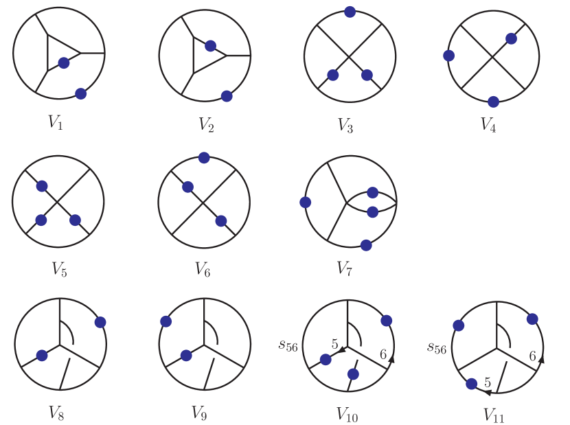
Figure 29: Four-loop vacuum diagrams describing the UV divergences of individual graphs in the four-loop ${\cal N}=4$ sYM amplitude. A dot indicates that a given propagator appears squared in the integral. For $V_{10}$ and $V_{11}$, the factor of $s_{56}$ indicates the insertion of $s_{56}=(l_{5}+l_{6})^{2}$ into the numerator of the integral, where lines 5 and 6 are marked in the figure.

The color factors of the 50 parent integrals in figs. 20–25 are collected in appendix C. For gauge group $SU(N_{c})$ it is straightforward to evaluate these color factors in the trace basis. We refrain from including these expressions directly, due to their length. (In appendix B we decompose the $C_{i}$ in a basis of color tensors for a general gauge group, and list the basis elements in trace basis.) However, the structure of the UV divergence is substantially simpler. Upon using the explicit color factors and the reduction to vacuum integrals (72), we find that the UV divergence of the color-dressed amplitude depends only on the three integrals $V_{1}$, $V_{2}$ and $V_{8}$:

$${\cal A}_{4}^{{(4)}}(1,2,3,4)\Bigr{|}^{SU(N_{c})}_{\rm pole} = -6\,g^{10}\,{\cal K}\,N_{c}^{2}\Bigl{(}N_{c}^{2}\,V_{1}+12\,(V_{1}+2\,V_{2}+V_{8})\Bigr{)}$$

$$\hskip-34.14322pt\hbox{}\times\Bigl{(}s_{12}\,(\,{\rm Tr}_{1324}+\,{\rm Tr}_{1423})+s_{23}\,(\,{\rm Tr}_{1243}+\,{\rm Tr}_{1342})+s_{13}\,(\,{\rm Tr}_{1234}+\,{\rm Tr}_{1432})\Bigr{)}\,.$$

Thus, we find that double-trace terms are absent from the divergence in the critical dimension $D_{c}$, as was the case at three loops. Another interesting feature is that terms independent of $N_{c}$ are also absent from the divergence. Only the leading and next-to-leading powers of $N_{c}$ are present in the single-trace divergence. Finally, using eqs. (V.2), (V.3) and (V.4), the divergences for $L=2,3,4$ all have the form,

$${\cal A}_{4}^{(L)}(1,2,3,4)\Bigr{|}^{SU(N_{c})}_{\rm pole} = (-1)^{L-1}\,(L-1)!\,g^{2L+2}\,{\cal K}\,N_{c}^{L}\biggl{(}\Bigl{(}1+\frac{12}{N_{c}^{2}}\Bigr{)}\,V^{\rm planar}+\frac{12}{N_{c}^{2}}\,V^{\rm non-planar}\biggr{)}$$ (74)

$$\hskip-28.45274pt\hbox{}\times\Bigl{(}s_{12}\,(\,{\rm Tr}_{1324}+\,{\rm Tr}_{1423})+s_{23}\,(\,{\rm Tr}_{1243}+\,{\rm Tr}_{1342})+s_{13}\,(\,{\rm Tr}_{1234}+\,{\rm Tr}_{1432})\Bigr{)}$$

$$\hskip 0.0pt\hbox{}+\delta_{L,2}\times(\hbox{double-trace-terms})\,,$$

where $V^{\rm planar}$ and $V^{\rm non-planar}$ come from planar and non-planar four-point integrals, respectively.

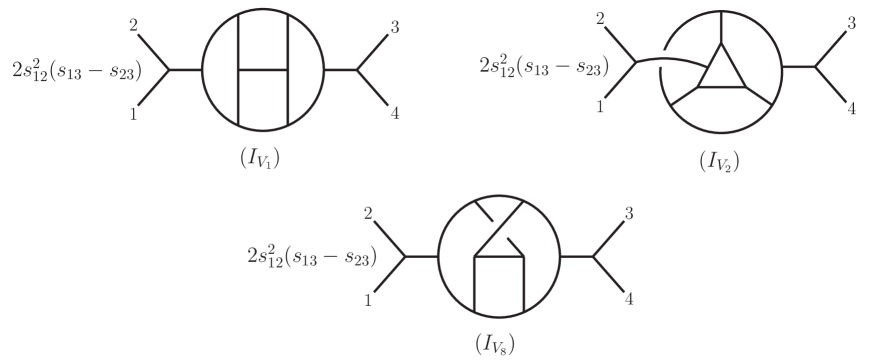
Figure 30: At four loops the leading divergence can be rearranged so that it comes from graphs with two spurious external propagators. The graphs with $1/s_{12}$ propagators are displayed here. This rearrangement makes manifest that the color factors of these graphs have no double-trace contributions. The complete contribution comes from summing over all 24 permutations of external legs and multiplication by a symmetry factor of $1/16$, $1/8$ and $1/16$, respectively, to remove double counts in both graphs.

For a general gauge group the leading UV divergence at four loops has a similarly simple structure, proportional to the tree-level color tensor:

$${\cal A}_{4}^{{(4)}}(1,2,3,4)\Bigr{|}^{G}_{\rm pole}=g^{10}\,{\cal K}\,{\cal V}^{(4)}\,\Bigl{(}s_{12}\,\tilde{f}^{a_{2}a_{3}b}\tilde{f}^{ba_{4}a_{1}}+s_{23}\,\tilde{f}^{a_{1}a_{2}b}\tilde{f}^{ba_{3}a_{4}}\Bigr{)}\,,$$ (75)

where

$${\cal V}^{(4)}=3\,(C_{V_{1}}V_{1}+2C_{V_{2}}V_{2}+C_{V_{8}}V_{8})\,.$$ (76)

The coefficients $C_{V_{1}}$, $C_{V_{2}}$ and $C_{V_{8}}$ are the group invariants associated with the corresponding vacuum diagrams. Their expressions in terms of structure constants are collected in appendix B. This structure is similar to that of the two- and three-loop UV poles in eqs. (67) and (68). As at three loops, the four-loop group invariants are not independent; rather, they satisfy the following relations:

$$C_{V_{1}}-C_{V_{2}} = \frac{C_{A}^{4}}{8}\,,$$ (77)

$$\frac{1}{3}C_{V_{1}}+\frac{2}{3}C_{V_{2}} = \frac{d_{A}^{abcd}d_{A}^{abcd}}{N_{A}}\,,$$ (78)

$$C_{V_{8}} = C_{V_{2}}\,.$$ (79)

As with the three-loop case discussed above, it is possible to rearrange the UV-divergent contributions at four loops into one-particle-reducible parent graphs. This form manifestly exhibits the absence of double-trace terms. In this case our representation exhibits two propagators in the same momentum channel, which are canceled by numerator factors, as depicted in fig. 30. The divergent part of the amplitude then has the simple form

$${\cal A}_{4}^{{(4)}}(1,2,3,4) = -g^{10}\,{\cal K}\sum_{S_{4}}\Bigl{[}{\textstyle\frac{1}{16}}C^{V_{1}}_{1234}I_{V_{1}}+{\textstyle\frac{1}{8}}\,C^{V_{2}}_{1234}I_{V_{2}}+{\textstyle\frac{1}{16}}C^{V_{8}}_{1234}I_{V_{8}}\Bigr{]}\;+\;\hbox{subleading}.$$

where the integrals correspond to the three graphs in fig. 30, and their color factors are proportional to the tree-level color factors,

$$C^{V_{i}}_{1234}\,=\,C_{V_{i}}\,\tilde{f}^{a_{1}a_{2}b}\tilde{f}^{ba_{3}a_{4}}\,,\qquad i=1,2,8.$$ (81)

The next step is to evaluate the UV poles for the four-loop vacuum integrals $V_{1}$, $V_{2}$ and $V_{8}$ in their critical dimension $D=11/2-2\epsilon$. To this end we use the same infrared rearrangement Vladimirov (related to the $R^{*}$ operation Rstar ) that was used CompactThree to evaluate the three-loop vacuum integrals $V^{{\rm(A)}}$ and $V^{{\rm(B)}}$: We inject and remove momentum $k^{\mu}$, with $k^{2}\neq 0$, at two of the vertices of the vacuum integral, thus transforming it into a four-loop two-point integral, which possesses the same UV poles, but no infrared divergences. (The infrared divergences arise in the small-momentum limit from doubled internal propagators.) We always take the two vertices in question to be connected by a single propagator. Then the four-loop two-point integral factorizes into the product of a finite three-loop two-point integral and a UV-divergent one-loop two-point integral.

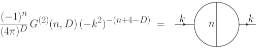
Figure 31: A two-loop integral with central propagator raised to the power $n$. If $n$ is not an integer, $G^{(2)}(n,D)$ cannot be reduced to one-loop integrals.

Some of the three-loop two-point integrals can be evaluated through a similar procedure, by factorizing them into a product of two-loop and one-loop two-point integrals. A few of the resulting two-loop integrals, such as those shown in fig. 31, are not factorizable. To evaluate them we employ the gluing relations CTIBP , which require consistency of the various ways of factorizing a higher-loop UV-divergent integral into products of lower-loop integrals.

For example, the diagram $V_{1}$ has four inequivalent propagators (not related by symmetry), leading to four inequivalent factorizations; they are shown in fig. 32. As usual, a dot indicates that a given propagator appears squared in the integral. Similarly, the numbers $(9-3D/2)$ and $(10-3D/2)$ indicate the power to which that propagator is raised, which is determined by dimensional analysis of the three-loop integral. All four factorizations should give the same answer; this consistency condition is an example of a gluing relation CTIBP .

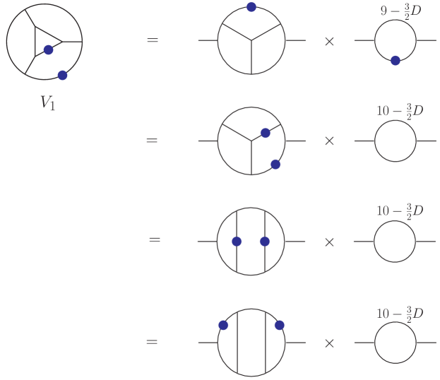
Figure 32: The UV poles in the vacuum diagram $V_{1}$ can be determined from the product of a finite three-loop two-point integral with a UV-divergent one-loop two-point integral. There are four inequivalent ways of doing the reduction, corresponding to different propagators connecting the two points at which the momentum $k^{\mu}$ is injected.

The one-loop bubble integral is simple to evaluate. For an arbitrary dimension $D$ and powers $n_{1}$ and $n_{2}$ of the two propagators, it is given by GrozinLectures

$$I^{\rm bubble}(n_{1},n_{2})\ \equiv-i\int\frac{d^{D}p}{(2\pi)^{D}}\frac{1}{\bigl{(}\,(p+k)^{2}\,\bigr{)}^{n_{1}}(p^{2}){\vphantom{\big{)}}}^{n_{2}}}\ =\ \frac{(-1)^{n_{1}+n_{2}}}{(4\pi)^{D/2}}G(n_{1},n_{2})(-k^{2})^{-(n_{1}+n_{2}-D/2)}\,,$$ (82)

where

$$G(n_{1},n_{2})\ =\ {\Gamma(-D/2+n_{1}+n_{2})\Gamma(D/2-n_{1})\Gamma(D/2-n_{2})\over\Gamma(n_{1})\Gamma(n_{2})\Gamma(D-n_{1}-n_{2})}\,.$$ (83)

In $D=11/2-2\epsilon$ dimensions, for the cases required in fig. 32 we have $(n_{1},n_{2})=(\textstyle{\frac{3}{4}}+3\epsilon,2)$ and $(n_{1},n_{2})=(\textstyle{\frac{7}{4}}+3\epsilon,1)$. Inserting these values into eq. (82) we find that both integrals have the same UV pole,

$$G({\textstyle{\frac{3}{4}}}+3\epsilon,2) = {4\over 21}{1\over\Gamma(\textstyle{\frac{3}{4}})}{1\over\epsilon}\ +\ {\cal O}(1)\,,$$ (84)

$$G({\textstyle{\frac{7}{4}}}+3\epsilon,1) = {4\over 21}{1\over\Gamma(\textstyle{\frac{3}{4}})}{1\over\epsilon}\ +\ {\cal O}(1)\,.$$ (85)

The finite three-loop two-point integrals can be reduced to a set of master integrals using the method of integration by parts (IBP) CTIBP , in particular the algorithm MINCER, which is available in FORM VermaserenFORM . For the two planar topologies occurring in fig. 32, the so-called Benz and ladder topologies, the IBP reduction procedure results in integrals that factorize into the product of two-loop and one-loop two-point integrals. Equation (82) can be applied to the latter. The two-loop integrals can also be reduced to products of one-loop integrals, except for the integrals $G^{(2)}(n,D)$ shown in fig. 31, in which the power $n$ to which the central propagator is raised is not an integer. However, a gluing relation can be used to solve for such integrals in $D=11/2$.

For example, IBP reduction of the top three lines in fig. 32 results in the following relations for the $1/\epsilon$ pole terms,

$$V_{1} = \Biggl{[}\frac{6272}{25}\,\Gamma^{5}({\textstyle{\frac{3}{4}}})-\frac{256}{5}\,\Gamma^{4}({\textstyle{\frac{3}{4}}})\Gamma({\textstyle{\frac{1}{2}}})\Gamma({\textstyle{\frac{1}{4}}})+8\,{\Gamma^{2}({\textstyle{\frac{3}{4}}})\Gamma({\textstyle{\frac{1}{4}}})\over\Gamma({\textstyle{\frac{1}{2}}})}G^{(2)}({\textstyle{\frac{9}{4}}},{\textstyle{\frac{11}{2}}})\biggr{]}{G({\textstyle{\frac{3}{4}}}+3\epsilon,2)\over(4\pi)^{11}}\quad{~{}}$$ (86)

$$= \Biggl{[}\frac{12992}{25}\,\Gamma^{5}({\textstyle{\frac{3}{4}}})-\frac{496}{5}\,\Gamma^{4}({\textstyle{\frac{3}{4}}})\Gamma({\textstyle{\frac{1}{2}}})\Gamma({\textstyle{\frac{1}{4}}})+\frac{1}{2}\,{\Gamma^{2}({\textstyle{\frac{3}{4}}})\Gamma({\textstyle{\frac{1}{4}}})\over\Gamma({\textstyle{\frac{1}{2}}})}G^{(2)}({\textstyle{\frac{9}{4}}},{\textstyle{\frac{11}{2}}})\biggr{]}{G({\textstyle{\frac{7}{4}}}+3\epsilon,1)\over(4\pi)^{11}}\qquad{~{}}$$ (88)

$$= \Biggl{[}\frac{12352}{25}\,\Gamma^{5}({\textstyle{\frac{3}{4}}})-\frac{288}{5}\,\Gamma^{4}({\textstyle{\frac{3}{4}}})\Gamma({\textstyle{\frac{1}{2}}})\Gamma({\textstyle{\frac{1}{4}}})-5\,{\Gamma^{2}({\textstyle{\frac{3}{4}}})\Gamma({\textstyle{\frac{1}{4}}})\over\Gamma({\textstyle{\frac{1}{2}}})}\Bigl{(}G^{(2)}({\textstyle{\frac{9}{4}}},{\textstyle{\frac{11}{2}}})-6\,G^{(2)}({\textstyle{\frac{5}{4}}},{\textstyle{\frac{11}{2}}})\Bigr{)}\biggr{]}$$

$$\hskip 5.69046pt\hbox{}\times{G({\textstyle{\frac{7}{4}}}+3\epsilon,1)\over(4\pi)^{11}}\,.\qquad{~{}}$$

Equating the three forms for $V_{1}$ at order $1/\epsilon$ yields

$$G^{(2)}({\textstyle{\frac{5}{4}}},{\textstyle{\frac{11}{2}}}) = -\frac{64}{25}\,\Gamma^{2}({\textstyle{\frac{3}{4}}})\Gamma^{2}({\textstyle{\frac{1}{2}}})+\frac{928}{125}\,{\Gamma^{3}({\textstyle{\frac{3}{4}}})\Gamma({\textstyle{\frac{1}{2}}})\over\Gamma({\textstyle{\frac{1}{4}}})}\ +\ {\cal O}(\epsilon)\,,$$ (89)

$$G^{(2)}({\textstyle{\frac{9}{4}}},{\textstyle{\frac{11}{2}}}) = -\frac{32}{5}\,\Gamma^{2}({\textstyle{\frac{3}{4}}})\Gamma^{2}({\textstyle{\frac{1}{2}}})+\frac{896}{25}\,{\Gamma^{3}({\textstyle{\frac{3}{4}}})\Gamma({\textstyle{\frac{1}{2}}})\over\Gamma({\textstyle{\frac{1}{4}}})}\ +\ {\cal O}(\epsilon)\,,$$ (90)

and

$$V_{1}={1\over(4\pi)^{11}\,\epsilon}\Biggl{[}\frac{512}{5}\,\Gamma^{4}({\textstyle{\frac{3}{4}}})-\frac{2048}{105}\,\Gamma^{3}({\textstyle{\frac{3}{4}}})\Gamma({\textstyle{\frac{1}{2}}})\Gamma({\textstyle{\frac{1}{4}}})\Biggr{]}\ +\ {\cal O}(1)\,.$$ (91)

The fourth line of fig. 32 provides a redundant equation.

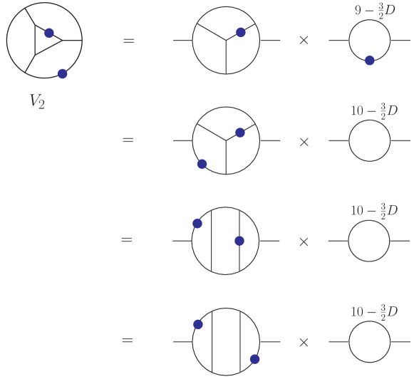
Figure 33: Four inequivalent ways of reducing vacuum diagram $V_{2}$ to a product of a finite three-loop two-point integral with a UV-divergent one-loop two-point integral.

A similar strategy leads to an analytic evaluation of $V_{2}$. As depicted in fig. 33, there are four inequivalent ways of factorizing this integral into a product of three-loop and one-loop two-point integrals. The same Benz and ladder topologies appear as for $V_{1}$, but with different configurations of double propagators. After using eqs. (89) and (90) for $G^{(2)}({\textstyle{\frac{5}{4}}},{\textstyle{\frac{11}{2}}})$ and $G^{(2)}({\textstyle{\frac{9}{4}}},{\textstyle{\frac{11}{2}}})$, they all give the same result,

$$V_{2}={1\over(4\pi)^{11}\,\epsilon}\Biggl{[}-\frac{4352}{105}\,\Gamma^{4}({\textstyle{\frac{3}{4}}})+\frac{832}{105}\,\Gamma^{3}({\textstyle{\frac{3}{4}}})\Gamma({\textstyle{\frac{1}{2}}})\Gamma({\textstyle{\frac{1}{4}}})\Biggr{]}\ +\ {\cal O}(1)\,.$$ (92)

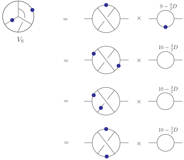
Figure 34: Four inequivalent ways of reducing vacuum diagram $V_{8}$ to a product of a finite non-planar three-loop two-point integral with a UV-divergent one-loop two-point integral.

There are four inequivalent ways of factorizing the non-planar vacuum integral $V_{8}$ into a product of three-loop and one-loop two-point integrals, depicted in fig. 34. This time the non-planar three-loop two-point topology is obtained. The IBP equations can be used to reduce any integral with this topology down to the master integral “NO_m” of the same topology, in which all propagators appear undoubled. In $D=4-2\epsilon$, gluing relations allow one to solve for the value of this master integral CTIBP as $\epsilon\to 0$ (which is proportional to $\zeta_{5}$). However, in $D=11/2$, we find that the gluing relations do not give new information. That is, all four ways of factorizing $V_{8}$ lead to the same expression,

$$V_{8}={1\over(4\pi)^{11}}{4\over 21}{1\over\Gamma({\textstyle{\frac{3}{4}}})}{V_{8}^{\rm fin}\over\epsilon}\ +\ {\cal O}(1)\,,$$ (93)

where

$$V_{8}^{\rm fin}=-\frac{5248}{125}\,\Gamma^{5}({\textstyle{\frac{3}{4}}})+\frac{224}{25}\,\Gamma^{4}({\textstyle{\frac{3}{4}}})\Gamma({\textstyle{\frac{1}{2}}})\Gamma({\textstyle{\frac{1}{4}}})+2\,{\rm NO}_{m}\,.$$ (94)

Although it is not needed for the four-loop ${\cal N}=4$ sYM amplitude, a similar factorization and reduction procedure for $V_{9}$ gives

$$V_{9}={1\over(4\pi)^{11}}{4\over 21}{1\over\Gamma({\textstyle{\frac{3}{4}}})}{V_{9}^{\rm fin}\over\epsilon}\ +\ {\cal O}(1)\,,$$ (95)

where

$$V_{9}^{\rm fin}=-\frac{15552}{125}\,\Gamma^{5}({\textstyle{\frac{3}{4}}})+\frac{576}{25}\,\Gamma^{4}({\textstyle{\frac{3}{4}}})\Gamma({\textstyle{\frac{1}{2}}})\Gamma({\textstyle{\frac{1}{4}}})-2\,{\rm NO}_{m}\,.$$ (96)

V.5 Gegenbauer sums for non-planar three-loop integral

Although we could not obtain an analytical value for $V_{8}$, or equivalently for $V_{9}$ or NO_m, we could obtain the result to 13 digits using the Gegenbauer polynomial $x$-space technique (GPXT) CKTGPXT . This method is based on the observation that, in position space, all propagators depend only on the coordinates of the vertices they connect and thus, after Wick rotation, they may be identified with the generation function of the Gegenbauer (or ultraspherical) polynomials. Expanding them and evaluating the integrals using properties of these polynomials reduces Feynman integrals to finitely many (nested) sums. A nice exposition of this technique is given in ref. Bekavac ; in particular the integral NO_m in any dimension $D$ is reduced to a triple sum. Using this approach for $D={\textstyle\frac{11}{2}}$, we obtain

$${\rm NO}_{m} = \frac{48}{50}\frac{\Gamma^{3}(\textstyle{\frac{3}{4}})}{\Gamma(\textstyle{\frac{1}{2}})}\sum_{\kappa=0}^{\infty}\frac{\Gamma(\kappa+\textstyle{\frac{7}{4}})}{\kappa!}\sum_{n=0}^{\infty}\frac{\Gamma(\textstyle{n+\kappa+\frac{7}{2}})}{\Gamma(\textstyle{n+\kappa+\frac{11}{4}})}\sum_{l=0}^{n}\frac{\Gamma(l+\textstyle{\frac{7}{4}})}{l!}\frac{\Gamma(n-l+\textstyle{\frac{7}{4}})}{(n-l)!}$$

$$\hskip 0.0pt\hbox{}\times\frac{1}{(l+\kappa+\textstyle{\frac{7}{4}})(n-l+\kappa+\textstyle{\frac{7}{4}})}\Biggl{[}-2\Biggl{(}\frac{1}{(n+\textstyle{\frac{1}{2}})(n+\kappa+\textstyle{\frac{5}{4}})(n+\kappa+\textstyle{\frac{11}{4}})(n+\kappa+2)}$$

$$\hskip 170.71652pt\hbox{}-\frac{1}{(n+3)(n+\kappa+\textstyle{\frac{5}{2}})(n+\kappa+\textstyle{\frac{13}{4}})(n+\kappa+4)}\Biggr{)}$$

$$\hskip 14.22636pt\hbox{}+\frac{n+2\kappa+\textstyle{\frac{11}{4}}}{(l+\kappa+1)(n-l+\kappa+1)}\Biggl{(}\frac{3n+4\kappa+\textstyle{\frac{17}{2}}}{(n+3)(n+\kappa+\textstyle{\frac{5}{2}})(n+\kappa+\textstyle{\frac{13}{4}})(n+2\kappa+\textstyle{\frac{7}{2}})}$$

$$\hskip 170.71652pt\hbox{}-\frac{3n+4\kappa+6}{(n+\textstyle{\frac{1}{2}})(n+\kappa+\textstyle{\frac{5}{4}})(n+\kappa+2)(n+2\kappa+\textstyle{\frac{7}{2}})}\Biggr{)}$$

$$\hskip 14.22636pt\hbox{}+\frac{n+2\kappa+\textstyle{\frac{17}{4}}}{(l+\kappa+\textstyle{\frac{5}{2}})(n-l+\kappa+\textstyle{\frac{5}{2}})}\Biggl{(}\frac{3n+4\kappa+\textstyle{\frac{23}{2}}}{(n+3)(n+\kappa+\textstyle{\frac{13}{4}})(n+\kappa+4)(n+2\kappa+\textstyle{\frac{7}{2}})}$$

$$\hskip 156.49014pt\hbox{}-\frac{3n+4\kappa+9}{(n+\textstyle{\frac{1}{2}})(n+\kappa+\textstyle{\frac{11}{4}})(n+\kappa+2)(n+2\kappa+\textstyle{\frac{7}{2}})}\Biggr{)}\Biggr{]}\,.$$

The sum over $l$ can be done in terms of hypergeometric functions:

$${\rm NO}_{m} = \frac{2^{5}}{5^{2}}\frac{\Gamma^{4}(\textstyle{\frac{3}{4}})}{\Gamma(\textstyle{\frac{1}{2}})}\sum_{n=0}^{\infty}\sum_{\kappa=0}^{\infty}A(\kappa,n)\biggl{[}$$

$$\hskip 0.0pt\hbox{}\Bigl{(}D(\kappa,n)-D(\kappa-{\textstyle{\frac{5}{4}}},n+{\textstyle{\frac{5}{2}}})-D(\kappa-{\textstyle{\frac{3}{4}}},n)+D(\kappa-2,n+{\textstyle{\frac{5}{2}}})\Bigr{)}H(\kappa,n)$$

$$\hskip-14.22636pt\hbox{}+\Bigl{(}D(\kappa,n)-D(\kappa-{\textstyle{\frac{5}{4}}},n+{\textstyle{\frac{5}{2}}})-D(\kappa+{\textstyle{\frac{3}{4}}},n)+D(\kappa-{\textstyle{\frac{1}{2}}},n+{\textstyle{\frac{5}{2}}})\Bigr{)}H(\kappa+{\textstyle{\frac{3}{2}}},n)\biggr{]}\,,$$

(98)

where

$$A(\kappa,n)=\frac{\Gamma(\kappa+{\textstyle{\frac{7}{4}}})\,\Gamma(n+{\textstyle{\frac{7}{4}}})\,\Gamma(\textstyle{n+\kappa+\frac{7}{2}})}{\kappa!\,n!\,\Gamma(\textstyle{n+{\kappa+\frac{11}{4}}})}\,,$$ (99)

$$D(\kappa,n)={1\over(\kappa+{\textstyle{\frac{3}{2}}})^{2}}\Biggl{[}{1\over n+{\textstyle{\frac{1}{2}}}}-{2\over(n+{\textstyle{\frac{1}{2}}})+(\kappa+{\textstyle{\frac{3}{2}}})}+{1\over(n+{\textstyle{\frac{1}{2}}})+2(\kappa+{\textstyle{\frac{3}{2}}})}\Biggr{]}\,,$$ (100)

and

$$H(\kappa,n)={1\over\kappa+1}\ {}_{3}F_{2}({\textstyle{\frac{7}{4}}},\kappa+1,-n;\kappa+2,-n-{\textstyle{\frac{3}{4}}};1)\,.$$ (101)

Using this representation and truncating the $\kappa$ and $n$ sums at a value $N$ up to 6500, we found sequences of truncated values NO${}_{m}(N)$, such as

$${\rm NO}_{m}(6000) = -6.197074209444889\,,\quad{\rm NO}_{m}(6100)=-6.197095923684655\,,$$

$${\rm NO}_{m}(6200) = -6.197116937698505\,,\quad{\rm NO}_{m}(6300)=-6.197137284819593\,,$$ (102)

$${\rm NO}_{m}(6400) = -6.197156996298421\,,\quad{\rm NO}_{m}(6500)=-6.197176101462998\,,$$

which we then fit to a polynomial in $1/N$, obtaining

$${\rm NO}_{m}=-6.198399226750(2),$$ (103)

where the number in parentheses indicates the uncertainty in the last digit.

We also applied GPXT to $V_{8}^{\rm fin}$ and $V_{9}^{\rm fin}$, obtaining similar sums, but with somewhat more complicated summands. The sequence for $V_{8}^{\rm fin}$ converges the fastest with $N$, but its numerical evaluation takes longer. We obtain,

$$V_{8}^{\rm fin} = 1.428452926283(3),$$ (104)

$$V_{9}^{\rm fin} = 2.472370645275(3).$$ (105)

To the given accuracy, these values are compatible with eq. (103) and the two analytic relations, eqs. (94) and (96).

The combination appearing in the subleading-color part of eq. (V.4) is

$$V_{1}+2V_{2}+V_{8}={1\over(4\pi)^{11}}{4\over 21}{1\over\Gamma({\textstyle{\frac{3}{4}}})}{6.161859216543(3)\over\epsilon}\,,$$ (106)

Thus the ratio of the subleading-color term to the leading-color term in eq. (V.4) is

$${12\,(V_{1}+2V_{2}+V_{8})\over N_{c}^{2}V_{1}}={44.40538395605(2)\over N_{c}^{2}}\,.$$ (107)

Amusingly, the large-$N_{c}$ approximation is strikingly bad, if we take the gauge group to be $SU(3)$ as in QCD. It is also strikingly bad at three loops, where the ratio analogous to eq. (107) can be extracted from eq. (V.3) and is very similar in magnitude, $36\,\zeta_{3}/N_{c}^{2}=(43.274\ldots)/N_{c}^{2}$.

The fact that these numerical ratios are irrational (in the four-loop case, apparently irrational) precludes the overall UV divergence from canceling for any gauge group $G$ at three or four loops, because ratios of group invariants are always rational.

VI UV divergences of subleading-color structures

As discussed in the previous section, the color double-trace terms are better behaved in the ultraviolet than the single-trace terms. Instead of the finiteness bound (41), for three and four loops the double-trace terms satisfy the bound (42). The double-trace terms of the three- and four-loop amplitudes are finite in the dimensions where the corresponding single-trace amplitudes first diverge, respectively in $D=6$ and $D=11/2$. This result implies that two-derivative double-trace operators of the form $\,{\rm Tr}({\cal D}^{2}F^{2})\,{\rm Tr}(F^{2})$ are not renormalized in these dimensions.

Suppose an $L$-loop cubic parent integral has $l$ powers of the loop momentum in the numerator factor $N_{i}$. Because it has $3L+1$ propagators in the denominator, it behaves in the UV as,

$$\sim\ \int{d^{DL}\ell\ \ell^{l}\over(\ell^{2})^{3L+1}}\ \sim\ \ell^{DL+l-6L-2}\,.$$ (108)

By dimensional analysis, the number of powers $m$ of external momenta sitting in front of this integral (including the four powers in the prefactor ${\cal K}$ defined in eq. (6)) is related to $l$ by $m=2L+2-l$. The critical dimension in which UV divergences can first appear in eq. (108) is found by setting $DL+l-6L-2=0$. Eliminating $l$ in factor of $m$, the critical dimension is

$$D(m,L)=4+\frac{m}{L}\,.$$ (109)

By Lorentz invariance, only even powers of momenta give nonvanishing results, implying that $m$ is effectively always even. Furthermore, the three- and four-loop integrals have at least six powers of external momenta that are manifest in the prefactors, counting the four powers in ${\cal K}$ and two powers in the “worst behaved” integral numerators $N_{i}$; therefore $m\geq 6$. We showed in the previous section that the divergences in the single-trace terms indeed start at $m=6$, with no further hidden cancellations. We also found cancellations in the double-traces terms in $D=4+6/L$. If there are no further cancellations, we expect the double-trace divergences to start with $m=8$, corresponding to $D=20/3$ for the three-loop double-trace terms, and implying $D=6$ for the four-loop double-trace terms.

An important question is whether the bound (42) is saturated for the double-trace terms, or whether further hidden cancellations remain. To definitively answer this question we must directly integrate our expressions, in order to extract the coefficients of the potential double-trace UV divergences in $D=20/3$ and $D=6$ at three and four loops, respectively. Below we answer this question at three loops.

VI.1 Extracting UV divergences

A systematic procedure for obtaining the potential divergences from multi-loop integrals is based on differentiating with respect to external momenta Vladimirov ; MarcusSagnotti . Here we follow a related procedure, and expand the amplitudes for small external momenta $k_{i}$. Formally this is achieved by introducing a single infinitesimal parameter $\varepsilon$, giving formal amplitudes $A(k_{i})\rightarrow A(\varepsilon k_{i})=\varepsilon^{6}a_{6}+\varepsilon^{7}a_{7}+\varepsilon^{8}a_{8}+\ldots$, where the expansion starts at $\varepsilon^{6}$ due to the manifest $m=6$ behavior of each integral. At the integrand level this expansion corresponds to,

$$I(k_{i},\ell_{j})\rightarrow I(\varepsilon k_{i},\ell_{j})=\varepsilon^{2}v_{6}+\varepsilon^{3}v_{7}+\varepsilon^{4}v_{8}+\ldots\,.$$ (110)

In eq. (110) we have dropped the overall tree factor ${\cal K}$, and the $v_{m}$ correspond to sums of vacuum-like integrands, depending only on the loop momenta $\ell_{j}$,

$$v_{m}=\sum_{p}\rho_{mp}(k_{i})\,{\cal V}_{p}(\ell_{j})\,,$$ (111)

where the dependence on the external momenta factorizes into polynomials $\rho_{mp}$ of degree $(m-4)$. The terms with odd powers of $\varepsilon$ in eq. (110) may be dropped because they are zero by Lorentz invariance. To make sense of the expansion under the integral sign, we formally take $\varepsilon|k_{i}|\ll|\ell_{j}|$ (where $|\cdot|$ is the Euclidean norm). This is not true in general, because the $\ell_{j}$ are integrated over all values. Fortunately, this error affects only the UV-finite part of the amplitude and is therefore not relevant to our discussion. The UV-divergent contributions indeed come from the region $|k_{i}|\ll|\ell_{j}|$ (if the amplitude contains no UV-divergent subdiagrams). We thus interpret the integrand expansion (110) as a formal series where the integrals over $v_{m}$ encode the UV divergence of the integral in dimension $D(m,L)$. If subdivergences appear, which happens for the potential color double-trace divergence at four loops, they must be accounted for; a procedure for doing so may be found in refs. Vladimirov ; MarcusSagnotti . Here we only evaluate the three-loop case, which has no subdivergences.

When evaluating terms in the expansion (110) one encounters tensor vacuum integrands that are not quite in the factorized form of eq. (111), but contain numerator factors in which external and loop momenta are contracted, of the form $k_{i}\cdot\ell_{j}$. These integrands are easily converted to the factorized form (111) using the identity,

$$\ell_{i}^{\mu}\ell_{j}^{\nu}\rightarrow\eta^{\mu\nu}\,\frac{\ell_{i}\cdot\ell_{j}}{D}\,.$$ (112)

This identity is valid for tensor vacuum integrals with two free space-time indices, which must be proportional to the metric tensor by Lorentz invariance. (Similar identities for tensors with more free indices are easily constructed, but we will not need them here.)

The various vacuum integrands ${\cal V}_{j}$ are distinguished by their propagator structure and possibly numerator factors $\ell_{i}\cdot\ell_{j}$, and can be represented as Feynman-like diagrams of various topologies. There are many hidden relations between the integrals, some of them generated by IBP identities CTIBP . These identities complicate the analysis slightly, because the representation of $v_{m}$ in terms of the ${\cal V}_{j}$, as given in eq. (111), is not unique. To expose the identities we can make use of the invariance of the integrals under reparametrizations,

$$\int\prod_{j=1}^{L}d^{D}\ell_{j}\,I\Bigl{(}\varepsilon k_{i},\ell_{j}\Bigr{)}=\int\prod_{j=1}^{L}d^{D}\ell_{j}\,I\Bigl{(}\varepsilon k_{i},\ell_{j}+\sum_{p}c_{jp}\varepsilon k_{p}\Bigr{)}\,,$$ (113)

where $c_{jp}$ are arbitrary numbers. After such a reparametrization the $\varepsilon$-expansion of the integrands look different, but the total UV pole after integration must be the same. We equate the different representations of $v_{m}$ integrals, for a sufficient number of reparametrized expansions of the form (113),

$$\int v_{m}=\sum_{p}\rho_{mp}\,V_{p}=\sum_{p}\rho^{\prime}_{mp}\,V_{p}=\ldots,$$ (114)

where $V_{p}$ stands for the integral of ${\cal V}_{p}$. The resulting system of linear equations for the poles of the $V_{j}$ can be solved easily. In contrast to IBP identities, the relations we find are between the pole parts of vacuum integrals that are relevant to our calculation, and no others.

VI.2 The logarithmic three-loop divergence in $D=20/3-2\epsilon$

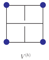
Figure 35: The three-loop vacuum diagram appearing in the UV divergence of the three-loop four-point ${\cal N}=4$ sYM amplitude in $D=20/3-2\epsilon$. Dots indicate the appearance of squared propagator factors in the integral.

Consider now the amplitude in $D=20/3$, which is the lowest dimension for which a potential divergence can appear in the three-loop color double-trace terms, and corresponds to the $v_{8}$ terms in eq. (110). In the expansion of the nine three-loop integrals we obtain 11 different scalar vacuum integrals. We will not present them explicitly here. However, we note that nine of them have a propagator topology very similar to the nine parent graphs of the three-loop amplitude, but where the external momenta is set to zero, $k_{i}\rightarrow 0$, effectively replacing a leg insertion by a two-point vertex, and thereby doubling a propagator. (An example is provided by $V^{(h)}$ in fig. 35.) The two remaining scalar vacuum diagrams both have a contact interaction. Remarkably, the consistency of the expansion (114) demands that the eleven vacuum integrals are all proportional to each other in $D=20/3$. The proportionality constants are simple rational numbers. We can therefore express the results in terms of the single vacuum-like diagram displayed in fig. 35. We obtain the following contributions to the three-loop divergence in $D=20/3-2\epsilon$,

$${\cal A}_{4}^{{(3)}}(1,2,3,4)\Bigr{|}_{\,{\rm Tr}_{1234}-\rm pole}^{(D=20/3)} = -g^{8}\,{\cal K}\,V^{(h)}\,{\rm Tr}_{1234}\,\Bigl{(}\frac{2}{5}N_{c}^{3}\,(7s^{2}+7t^{2}+6u^{2})$$ (116)

$$\qquad\qquad\qquad\quad\;\hbox{}-\frac{5}{2}N_{c}\,{}(23s^{2}+23t^{2}-126u^{2})\Bigr{)}\,,$$

$${\cal A}_{4}^{{(3)}}(1,2,3,4)\Bigr{|}_{\,{\rm Tr}_{12}\,{\rm Tr}_{34}-\rm pole}^{(D=20/3)} = -g^{8}\,{\cal K}\,V^{(h)}\,{\rm Tr}_{12}\,{\rm Tr}_{34}\Bigl{(}7N_{c}^{2}\,(58s^{2}+3t^{2}+3u^{2})$$ (118)

$$\qquad\qquad\qquad\qquad\;\hbox{}+400\,(s^{2}+t^{2}+u^{2})\Bigr{)}\,,$$

where we have isolated the pieces of the divergence proportional to two characteristic four-point color structures of $SU(N_{c})$: the single trace $\,{\rm Tr}_{1234}$ and double trace $\,{\rm Tr}_{12}\,{\rm Tr}_{34}$, respectively. The divergences of all other single- and double-trace structures are simply related to eq. (116) and eq. (118) by crossing symmetry. This proves that no further cancellations remain in the double-trace terms and at least for $L=3$, the finiteness formula (42) is saturated. The scalar vacuum integral appearing in eq. (116) and eq. (118) is shown in fig. 35, and the UV divergence is given by,

$$V^{(h)}=-{1\over(4\pi)^{10}}{\Gamma^{3}(-\textstyle{\frac{2}{3}})\over 2310\,\epsilon}\ +\ {\cal O}(1)\,.$$ (119)

We can similarly determine the $D=20/3$ logarithmic divergence for a general gauge group $G$. For clarity, we split up the divergence into two contributions: one containing the tree color tensors and one containing the irreducible loop color tensors (the latter was shown to be finite in $D=6$). The result is,

$${\cal A}_{4}^{{(3)}}(1,2,3,4)\Bigr{|}_{\rm tree\hbox{-}pole}^{(D=20/3)} = -\frac{1}{320}g^{8}\,{\cal K}\,V^{(h)}\Bigl{[}b_{1}^{(0)}\Bigl{(}200C_{V^{{\rm(B)}}}(7s^{2}-94t^{2}+7u^{2})$$ (120)

$$\hbox{}\hskip 113.81102pt-16C_{A}^{3}(7s^{2}+6t^{2}+7u^{2})\Bigr{)}$$

$$\hbox{}\hskip 65.44142pt-b_{2}^{(0)}\Bigl{(}200C_{V^{{\rm(B)}}}(14s^{2}-87t^{2}-87u^{2})$$

$$\hbox{}\hskip 113.81102pt+16C_{A}^{3}(6s^{2}+7t^{2}+7u^{2})\Bigr{)}\Bigr{]}\,,$$

$${\cal A}_{4}^{{(3)}}(1,2,3,4)\Bigr{|}_{\rm loop\hbox{-}pole}^{(D=20/3)} = -\frac{1}{24}g^{8}\,{\cal K}\,V^{(h)}\Bigl{[}21b_{1}^{(1)}C_{A}^{2}(3s^{2}+3t^{2}+58u^{2})+770b_{2}^{(2)}C_{A}(t^{2}-u^{2})$$

$$\hbox{}-70b_{1}^{(2)}C_{A}(9s^{2}+20t^{2}+31u^{2})+1200b_{1}^{(3)}(s^{2}+t^{2}+u^{2})\Bigr{]}\,,$$

where the basis color tensors $b_{i}^{(L)}$ can be found in appendix B. For the three-loop four-point amplitude, any color tensor can be written in terms of the six basis tensors that feature in the above formulæ. Note that none of the coefficients of the basis elements vanish. The full divergence is simply the sum of the tree (120) and loop (LABEL:3loopGloop) color-tensor contributions. Note also that this division into tree and loop contributions is somewhat arbitrary, and certainly not unique (unless the loop contribution vanishes, as in the case of the three-loop divergence in $D=6$); it depends on the choice of basis for the color tensors. (Specifically, choosing different basis tensors $b_{i}^{(L)}$ at $L$ loops affects the coefficients of the $b_{i}^{(L)}$ tensors, as well as of lower-loop basis tensors, but not the coefficients of higher-loop basis tensors.) The split in eqs. (120) and (LABEL:3loopGloop) does not even respect the Bose symmetry of the divergence.

By inspecting the above expressions, it is clear that at three loops the coefficients of all independent color tensors, for $SU(N_{c})$ as well as for a general group $G$, develop UV divergences in $D=20/3$. In other words, the double-trace terms for $SU(N_{c})$, and the loop color-tensor terms for general $G$, which are finite in $D=6$, exhibit no further cancellations; their divergences start at $m=8$, or equivalently at $D=20/3$.

Here we will not evaluate the four-loop divergence in $D=6$. Its evaluation is more involved than that of the three-loop case, not only because of the greater complexity of the four-loop integrands, but also because of a three-loop subdivergence. A calculation of the divergences in $D=6$ would, of course, answer the question of whether there may be further hidden UV cancellations in the four-loop double-trace terms.

VII Conclusions

In this paper we obtained the four-loop four-point amplitude of ${{\cal N}=4}$ super-Yang-Mills theory, i.e. both the planar and the non-planar contributions, in terms of a set of 50 loop integrals (one of which has vanishing color coefficient and also integrates to zero). The planar part of the amplitude was already known BCDKS . Here we presented the more complicated non-planar terms. At the core of our computation lies the unitarity method UnitarityMethod , and in particular the method of maximal cuts BCDKS ; FiveLoop . For the planar amplitude, hidden symmetries MagicIdentities lead to major simplifications. No comparable considerations are presently available for the non-planar terms.

An important problem is therefore to develop new tools for constructing multi-loop integrands, which are valid also for non-planar amplitudes. In this paper we extended and developed graphical rules applicable to such amplitudes, to speed up their construction. The simplest of these rules is a generalization of the rung rule BRY ; BDDPR , which allows us to write down all contributions having two-particle cuts directly from lower-loop results. However, not all terms have two-particle cuts. A more powerful tool, which partly bypasses this limitation, is the box cut, which yields terms having four-point subgraphs. This rule has a simple graphical formulation. Another rule, based on the color-kinematic duality BCJ , allows us to generate many non-planar contributions from much simpler planar ones. In fact, it appears that these relations can be applied directly at loop level with no cut conditions imposed, though this has been confirmed only through three loops BCJLoop . Although the graphical rules presented in this paper do not determine all contributions, they determine most terms, allowing us to focus on the remaining ones, for which we employed generalized unitarity, in particular maximal and near-maximal cuts. Nevertheless, identifying further tools and structures would be extremely helpful for future studies.

The results in this paper, as well as those of refs. GravityThree ; FiveLoop ; CompactThree ; GravityFour , provide a wealth of information on the explicit form of planar and non-planar amplitudes in ${\cal N}=4$ sYM. However, the structures we are seeking, which could allow the development of new tools, are obscured by ambiguities in assigning contact terms to the parent graphs. Each form of the amplitude may expose one property or structure while hiding others. For example, the representations of the complete three- and four-loop four-point amplitudes presented in this paper do not highlight the fact that double-trace terms are better behaved in the UV than single-trace terms. As we discussed, a nontrivial rearrangement is necessary to manifestly expose this feature. As another example, nontrivial rearrangements would be needed to expose a recently proposed loop-level color-kinematics duality in the four-loop four-point ${\cal N}=4$ sYM amplitude. It is quite likely that other important features will be revealed through appropriate reorganizations of the amplitudes.

Generally it is simplest to construct an ansatz for the amplitude in four dimensions, where powerful helicity and on-shell superspace methods can be used. Because we are interested in the higher-dimensional UV structure of the theory, it is important that our construction of the four-loop amplitude be valid in higher dimensions. In this paper, we evaluated a complete set of cuts in four dimensions, but only an incomplete set in $D$ dimensions. Strong checks that our expressions are valid in $D$ dimensions come from two-particle cuts, box cuts, and the color-kinematic duality BCJ . The planar contributions to the four-loop four-point amplitude have been evaluated in $D$ dimensions, subject only to the mild condition that no terms violate the expected power count BCDKS . It is nevertheless still important to compare our results against a complete evaluation of the $D$-dimensional cuts. At least in $D=6$, efficient tools for doing so now exist OConnell ; SixDimSusy ; FutureD6 .

A key reason for computing the four-loop ${\cal N}=4$ sYM amplitude is to study its UV behavior as a function of dimension. Our expressions are manifestly finite for $D<11/2$ in accordance with the expectation BDDPR ; HoweStelleRevisited that $L$-loop ${\cal N}=4$ sYM amplitudes are finite for $D<4+6/L$. Direct evaluation of the integrals reveals that the theory is indeed UV divergent in $D=11/2$ for a general non-abelian gauge group $G$; we have therefore demonstrated that no hidden UV cancellations remain for generic $G$, through at least four loops.

In the course of our analysis of the color structure of UV divergences, we have found, however, that certain terms are more convergent than the general expectation: in particular, for $G=SU(N_{c})$ the terms with double-trace color factors have no divergences in the critical dimension for which single-trace divergences first appear, at three and four loops DurhamAndCopenhagenTalks . This curious improved behavior has been discussed from the vantage point of the pure-spinor formalism in string theory DoubleTraceBerkovits and field theory BG2010 , as well as from the standpoint of field-theoretic algebraic non-renormalization theorems DoubleTraceNonrenormalization . In the present paper, we give a field-theoretic clarification, motivated by the structure of the leading contributions in the string theory analysis of ref. DoubleTraceBerkovits : It is possible to rearrange all leading-divergence contributions of the amplitude into a one-particle-reducible form, which has propagators depending only on external momenta. The color dressing of such terms forbids the presence of double-trace color factors. In contrast to the string-based approach, this also clarifies the absence of subleading-color double-trace terms. This rearrangement can first be performed at three loops because this is the first loop order where inverse propagators can appear in numerators of integrals. The first potential divergence of double-trace terms is then at $D=4+8/L$, in contrast to the $D=4+6/L$ divergences for single-trace terms. We showed that the $D=4+8/L$ bound is saturated at three loops; it remains an interesting open question whether it is saturated at four loops.

An equally thorough understanding of the UV properties of ${{\cal N}=8}$ supergravity is absent. However, the complete four-loop four-point amplitude constructed in this paper helps shed light on this issue. This is another important motivation for our work. The ${\cal N}=4$ sYM amplitude is the basic input into the construction of the corresponding ${{\cal N}=8}$ supergravity amplitude GravityFour , following the strategy of refs. BDDPR ; GravityThree ; CompactThree : as a consequence of generalized unitarity GeneralizedUnitarity ; TwoLoopSplit and of the KLT KLT and graphical numerator double-copy relations BCJ , cuts of ${{\cal N}=8}$ supergravity amplitudes can be expressed directly in terms of the cuts of ${\cal N}=4$ sYM amplitudes. Although ${{\cal N}=8}$ supergravity is known to have surprisingly good UV properties BDDPR ; Finite ; DualityArguments ; HoweStelleRevisited ; Berkovits ; GravityThree ; CompactThree ; BHS ; GravityFour and may even be UV finite Finite , its UV behavior beyond four loops is still unclear. Recently, a consensus has formed UnExpectedCancel ; DoubleTraceBerkovits ; DoubleTraceNonrenormalization ; GRV2010 ; FreedmanCounterTerms ; KalloshRamond ; Vanhove2010 that supersymmetry alone cannot protect the theory beyond seven loops in $D=4$ and that an additional mechanism must be at play if the theory is finite. Clearly, further high loop studies would be helpful for resolving this issue. Apart from its direct relevance for answering the question of ultraviolet finiteness of ${{\cal N}=8}$ supergravity, ${\cal N}=4$ sYM offers a much simpler arena for sharpening our understanding of such divergences in supersymmetric theories, as well as for explicitly testing general arguments.

The results described in this paper may also shed light on the infrared singularities of gauge-theory amplitudes, by allowing tests of proposed structures for the soft anomalous-dimension matrix CompactThree ; BN ; GM and the cusp anomalous dimension. The evaluation of the non-planar integrals appearing in the expression of the amplitude in $D=4-2\epsilon$ is a necessary step for the extraction of its infrared divergences. Unfortunately, such four-point integrals are notoriously difficult to evaluate; they have not been computed even at three loops. Thus, the use of our results for this purpose must await the development of new techniques for evaluating higher-loop non-planar integrals.

In summary, the results and tools presented here should provide new handles on a number of important unanswered questions, including the structure of multi-loop infrared divergences in gauge theories and the UV properties of gravity theories. They may also help expose hitherto unexpected structures in these theories.

Appendix A Sample evaluation of a non-planar cut

In this appendix we describe the details of the evaluation of a nontrivial cut which appears in the construction of eq. (40). The cut presented here can be used to confirm large parts of our construction, and is sensitive to the most complicated non-planar terms in the amplitude. Seven-particle cuts, which break the four-loop amplitude into four- and five-point MHV and $\overline{\hbox{MHV}}$ tree amplitudes are especially helpful in our construction, because they are sensitive to all terms actually present in the amplitudes, and yet are relatively simple to work with. As mentioned in the text, we checked that our expression for the amplitudes matches all such cuts.

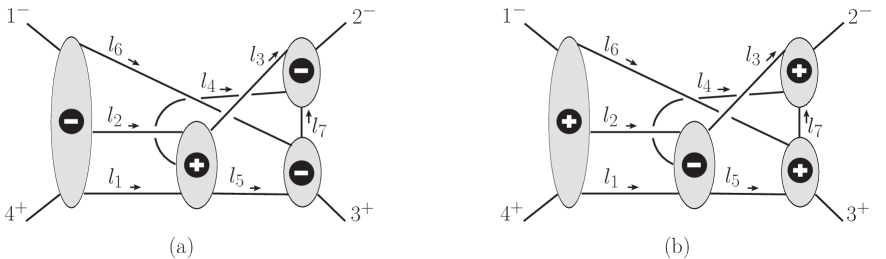
Figure 36: A nontrivial non-planar cut at four loops. The cuts (a) and (b) represent the two distinct internal helicity configurations contributing to this seven-particle cut. The blobs representing MHV trees are labeled by a “$+$” and the blobs representing $\overline{\hbox{MHV}}$ blobs are labeled by a “$-$”. For a four-point amplitude either assignment can be made; the assignment in the figure makes the supersum calculation most transparent.

Here we present the steps necessary to test eq. (40) and the numerator factors assigned to the integrals, using the seven-particle cut displayed in fig. 36. This cut has already been discussed in considerable detail in sect. 6C of ref. SuperSum , so here we will simply quote the result, and focus instead on the cut of our result in eq. (40). As noted in fig. 36, the contributions to the cut comes in two distinct sectors, depending on the configuration of MHV and $\overline{\hbox{MHV}}$ assignment of the tree amplitudes composing the cut. The fact that all factors of tree amplitudes are either MHV or $\overline{\hbox{MHV}}$ leads to compact expressions for these two components. From ref. SuperSum , we have the simplified result:

$$C^{\ref{AppFourLoopNonPlanarExampleFigure}\rm(a)} = \sum_{\rm states}A_{5}^{\overline{\rm MHV}}(1^{-},l_{6},l_{2},l_{1},4^{+})\,A_{5}^{{\rm MHV}}(-l_{1},l_{4},-l_{2},l_{3},l_{5})\,$$

$$\hbox{}\times A_{4}(-l_{4},-l_{3},2^{-},-l_{7})\,A_{4}(-l_{5},-l_{6},l_{7},3^{+})$$

$$= \big{(}\left\langle 1\,2\right\rangle\left[l_{7}\,2\right]\left[l_{6}\,3\right]\left[1\,4\right]\big{)}^{4}\frac{1}{[41][1l_{6}][l_{6}l_{2}][l_{2}l_{1}][l_{1}4]}$$

$$\hbox{}\times\frac{1}{\left\langle l_{1}\,l_{4}\right\rangle\left\langle l_{4}\,l_{2}\right\rangle\left\langle l_{2}\,l_{3}\right\rangle\left\langle l_{3}\,l_{5}\right\rangle\left\langle l_{5}\,l_{1}\right\rangle}\frac{1}{[3l_{5}][l_{5}l_{6}][l_{6}l_{7}][l_{7}3]}\frac{1}{[2l_{7}][l_{7}l_{4}][l_{4}l_{3}][l_{3}2]}\,,$$

$$C^{\ref{AppFourLoopNonPlanarExampleFigure}\rm(b)} = \sum_{\rm states}A_{5}^{{\rm MHV}}((1^{-},l_{6},l_{2},l_{1},4^{+})\,A_{5}^{\overline{\rm MHV}}(-l_{1},l_{4},-l_{2},l_{3},l_{5})\,$$ (122)

$$\hbox{}\times A_{4}(-l_{4},-l_{3},2^{-},-l_{7})\,A_{4}(-l_{5},-l_{6},l_{7},3^{+})$$

$$= \big{(}\left\langle 1\,2\right\rangle\left[2\,3\right]\left[l_{3}\,l_{4}\right]\left[l_{5}\,l_{7}\right]\big{)}^{4}\frac{1}{\left\langle 4\,1\right\rangle\left\langle 1\,l_{6}\right\rangle\left\langle l_{6}\,l_{2}\right\rangle\left\langle l_{2}\,l_{1}\right\rangle\left\langle l_{1}\,4\right\rangle}$$ (124)

$$\hbox{}\times\frac{1}{[l_{1}l_{4}][l_{4}l_{2}][l_{2}l_{3}][l_{3}l_{5}][l_{5}l_{1}]}\frac{1}{[3l_{5}][l_{5}l_{6}][l_{6}l_{7}][l_{7}3]}\frac{1}{[2l_{7}][l_{7}l_{4}][l_{4}l_{3}][l_{3}2]}\,.$$

This simple result is determined by the purely gluonic configurations crossing the cuts; in the first case there are seven such configurations and in the second eight.

The above two expressions are related by complex conjugation:

$$\frac{C^{\ref{AppFourLoopNonPlanarExampleFigure}\rm(b)}}{A^{\rm tree}_{4}}=\Biggl{(}\frac{C^{\ref{AppFourLoopNonPlanarExampleFigure}\rm(a)}}{A^{\rm tree}_{4}}\Biggr{)}^{\dagger}\,.$$ (125)

This relation guarantees from the outset that after dividing by the tree amplitude, the sum of the two expressions is a function of only Lorentz dot products, with all spinors or Levi-Civita tensors dropping out. (This property is special to four-point amplitudes and does not hold for higher-point amplitudes.)

The cut in eq. (124) needs to be compared to the cut of our expression for the four-loop amplitude in eq. (40). To identify the possible contributions to this cut we write out all possible tree graphs with only three-point vertices, for the tree amplitudes composing the cut. These are depicted in fig. 36. (We need only track graphs with three-vertices, following our organization of contributions according to such graphs.) The graphs labeled by (a) and (b) correspond to the two five-point amplitudes in the cut, and those labeled by (c) and (d) to the four-point amplitudes. Two graphs were dropped from (a), in which external legs 1 and 4 fuse together, because they would generate three-point subgraphs, which we know do not occur.

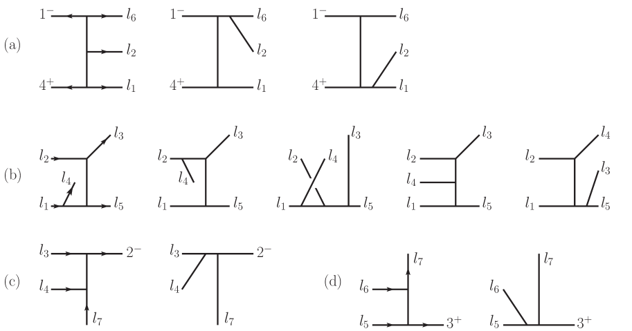
Figure 37: Tree structures building up the cut in fig. 36.

After sewing together the four trees, we can identify the integrals and labelings of internal and external lines that contribute to this cut. Of the 60 possible such products, 22 may be ignored as they do not appear in the list of integrals composing the answer. The unnecessary ones would have triangle or bubble subgraphs, and would violate the known no-triangle property of ${\cal N}=4$ sYM at one, two or three loops. Organized in this way, the contributions to the cut in fig. 36 are listed in table 1, which is structured as follows. The first column represents the product of trees — $(ijkl)$ standing for the product of the $i$th tree from fig. 37(a), the $j$th tree from figure 37(b), the $k$th tree from fig. 37(c) and the $l$th tree from fig. 37(d). The second column is the number $n$ of the integral ${\cal I}_{n}$ for which $(ijkl)$ represents a cut contribution. A given integral may appear multiple times in the same cut, Several such products may represent cuts of the same integral. The third column contains the mapping of (internal and external) momenta between figs. 20–25 and the momenta of the tree amplitudes assigned in figs. 36 and 37. The last column represents the numerator factors from figs. 20–25, evaluated for the cut conditions specified in fig. 36. We specify the mapping only for the external momenta or when the numerator contains a given internal momentum. For convenience we have introduced the notation,

$$k_{i,j}=k_{i}+k_{j}\,,\hskip 56.9055ptl_{i,j}=l_{i}+l_{j}\,,\hskip 56.9055ptl_{i,\bar{j}}=l_{i}-l_{j}\,,$$ (126)

$$\hskip 56.9055ptl_{i,j,m}=l_{i}+l_{j}+l_{m}\,,\hskip 56.9055ptl_{i,\bar{j},\bar{m}}=l_{i}-l_{j}-l_{m}\,.$$ (127)

In general, subscripts separated by commas denote sums of momenta, while a bar over the subscripts denotes that the sign of the corresponding momentum is minus.

In table 1 there are a total of 38 contributions to the cut. The first such contribution is

$$C^{(1321)}={\cal K}\,{-(k_{2}+l_{5}-l_{7})^{2}[s_{13}(k_{2}+l_{5}-l_{7})^{2}-s_{23}(k_{1}+k_{3}+l_{7})^{2}]\over(k_{1}+l_{6})^{2}(l_{1}+k_{4})^{2}(l_{4}-l_{1})^{2}(l_{3}+l_{5})^{2}(l_{3}+l_{4})^{2}(l_{5}-k_{3})^{2}}\,,$$ (128)

where the numerator is given in table 1 and the denominators can be read off from the propagators of the diagrams in fig. 37. We have put back the overall prefactor $\cal K$ defined in eq. (6). The reader may check that the sum over all 38 contributions adds up to give the sum of the two contributions in eq. (124). It is convenient to make this comparison numerically, but it is also straightforward to carry out analytically after imposing momentum conservation.

Table 1: The numerator factors and tree structures appearing in the seven particle cut of fig. 36. The first column gives the tree structure according to fig. 36 and the notation described in the text. The second column gives the integral number $n$ whose cut gives the tree structure. The third column gives the relabelings needed to go from the integral labels to the cut labels. The last column gives the numerator factors in the labeling of the cut. The associated propagator factors can be read off from the tree structures.

Trees	${\cal I}_{n}$	Momentum relabeling	Numerator factor
$(1321)$	34	$k_{1}\rightarrow k_{3},$ $k_{2}\rightarrow k_{1},$ $k_{3}\rightarrow k_{4},$ $k_{4}\rightarrow k_{2},$ $l_{5}\rightarrow k_{2}-l_{7},$ $l_{6}\rightarrow l_{5}$	$-(k_{2}+l_{5,\overline{7}})^{2}[s_{13}(k_{2}+l_{5,\overline{7}})^{2}-s_{23}(k_{1,3}+l_{7})^{2}]$
$(1322)$	18	$k_{1}\rightarrow k_{2},$ $k_{2}\rightarrow k_{3},$ $k_{3}\rightarrow k_{1},$ $k_{4}\rightarrow k_{4},$ $l_{5}\rightarrow k_{3}+l_{7},$ $l_{6}\rightarrow k_{1}+l_{6},$ $l_{7}\rightarrow l_{4}$	$s_{23}(k_{1,3}+l_{7})^{2}(k_{1,4}+l_{6})^{2}$
$(3412)$	18	$k_{1}\rightarrow k_{4},$ $k_{2}\rightarrow k_{1},$ $k_{3}\rightarrow k_{3},$ $k_{4}\rightarrow k_{2},$ $l_{5}\rightarrow-l_{6},$ $l_{6}\rightarrow-l_{7},$ $l_{7}\rightarrow-l_{2}$	$~{}s_{14}(k_{3}-l_{6})^{2}(k_{2}-l_{7})^{2}$
$(1522)$	20	$k_{1}\rightarrow k_{2},$ $k_{2}\rightarrow k_{3},$ $k_{3}\rightarrow k_{4},$ $k_{4}\rightarrow k_{1},$ $l_{5}\rightarrow l_{3,5},$ $l_{6}\rightarrow l_{4},$ $l_{7}\rightarrow k_{3}+l_{7}$	$~{}\,s_{23}\,l_{3,4,5}^{2}(k_{1,3}+l_{7})^{2}$
$(3212)$	20	$k_{1}\rightarrow k_{4},$ $k_{2}\rightarrow k_{1},$ $k_{3}\rightarrow k_{2},$ $k_{4}\rightarrow k_{3},$ $l_{5}\rightarrow-l_{1,{\overline{5}}},$ $l_{6}\rightarrow-l_{2},$ $l_{7}\rightarrow-l_{6}$	$~{}\,s_{14}l_{\overline{1},\overline{2},5}^{2}(k_{3}-l_{6})^{2}$

Trees	${\cal I}_{n}$	Momentum relabeling	Numerator factor
$(2212)$	25	$k_{1}\rightarrow k_{4},$ $k_{2}\rightarrow k_{1},$ $k_{3}\rightarrow k_{2},$ $k_{4}\rightarrow k_{3},$ $l_{6}\rightarrow-l_{2},$ $l_{7}\rightarrow-l_{1},$ $l_{8}\rightarrow-l_{1,{\bar{5}}},$ $l_{9}\rightarrow-l_{7}$	$~{}\,s_{14}[(k_{2}-l_{1})^{2}l_{\bar{1},\bar{2},5}^{2}-s_{14}(l_{\bar{1},5}+k_{2})^{2}]$
$(2412)$	25	$k_{1}\rightarrow k_{1},$ $k_{2}\rightarrow k_{4},$ $k_{3}\rightarrow k_{2},$ $k_{4}\rightarrow k_{3},$ $l_{6}\rightarrow-l_{1,{\bar{5}}},$ $l_{7}\rightarrow-l_{2,6},$ $l_{8}\rightarrow-l_{2},$ $l_{9}\rightarrow-l_{7}$	$\,-s_{14}[{}(k_{2}-l_{2,6})^{2}(l_{5}-l_{1,2})^{2}-s_{14}(k_{2}-l_{2})^{2}]$ $\hbox{}+s_{14}l_{5,\bar{1}}^{2}(k_{2}-l_{2,6})^{2}$
$(1511)$	33	$k_{1}\rightarrow k_{4},$ $k_{2}\rightarrow k_{1},$ $k_{3}\rightarrow k_{3},$ $k_{4}\rightarrow k_{2},$ $l_{5}\rightarrow l_{3,5},$ $l_{6}\rightarrow l_{4},$ $l_{7}\rightarrow l_{5},$ $l_{8}\rightarrow-l_{7},$ $l_{9}\rightarrow k_{3}-l_{5},$ $l_{10}\rightarrow l_{4,7},$ $l_{11}\rightarrow k_{1}+l_{6},$ $l_{12}\rightarrow-l_{6}$	$s_{14}[l_{3,5}^{2}(k_{1,3}-l_{5})^{2}+l_{5,\bar{7}}^{2}(k_{4}+l_{3,5})^{2}]$ $\hbox{}-l_{3,4,5}^{2}[s_{23}(k_{1,3}-l_{5})^{2}-s_{13}(k_{3}+l_{4,\bar{5},7})^{2}+s_{13}l_{4,7}^{2}]$
$(1312)$	33	$k_{1}\rightarrow k_{4},$ $k_{2}\rightarrow k_{1},$ $k_{3}\rightarrow k_{3},$ $k_{4}\rightarrow k_{2},$ $l_{5}\rightarrow l_{4},$ $l_{6}\rightarrow l_{3,5},$ $l_{7}\rightarrow-l_{7},$ $l_{8}\rightarrow l_{5},$ $l_{9}\rightarrow k_{3}+l_{7},$ $l_{10}\rightarrow l_{3},$ $l_{11}\rightarrow k_{1}+l_{6},$ $l_{12}\rightarrow-l_{6}$	$\,l_{3,4,5}^{2}[s_{14}(k_{1,3}+l_{7})^{2}-s_{13}(k_{3}+l_{3,7})^{2}]$ $\hbox{}-s_{14}(k_{4}+l_{4})^{2}l_{5,\bar{7}}^{2}$

Trees	${\cal I}_{n}$	Momentum relabeling	Numerator factor
$(1412)$	33	$k_{1}\rightarrow k_{2},$ $k_{2}\rightarrow k_{3},$ $k_{3}\rightarrow k_{1},$ $k_{4}\rightarrow k_{4},$ $l_{5}\rightarrow-l_{2},$ $l_{6}\rightarrow-l_{1,{\bar{5}}},$ $l_{7}\rightarrow k_{1}+l_{6},$ $l_{8}\rightarrow l_{5},$ $l_{9}\rightarrow-l_{6},$ $l_{10}\rightarrow-l_{1},$ $l_{11}\rightarrow-l_{7},$ $l_{12}\rightarrow k_{3}+l_{7}$	$-(l_{5}-l_{1}-l_{2})^{2}[s_{13}(l_{6}+l_{1})^{2}-s_{23}(k_{3}-l_{6})^{2}]$ $\hbox{}-s_{23}(k_{2}-l_{2})^{2}(k_{1}+l_{5}+l_{6})^{2}$
$(1311)$	36	$k_{1}\rightarrow k_{2},$ $k_{2}\rightarrow k_{3},$ $k_{3}\rightarrow k_{1},$ $k_{4}\rightarrow k_{4},$ $l_{5}\rightarrow l_{4},$ $l_{6}\rightarrow l_{5},$ $l_{7}\rightarrow k_{1}+l_{6},$ $l_{8}\rightarrow k_{3}-l_{5},$ $l_{9}\rightarrow l_{4,7},$ $l_{10}\rightarrow-l_{7},$ $l_{11}\rightarrow l_{3,5},$ $l_{12}\rightarrow-l_{6}$	$s_{14}(k_{1}+l_{6})^{2}(k_{2}-l_{4})^{2}-l_{5,\bar{7}}^{2}s_{14}(k_{4}+l_{4})^{2}$ $\hbox{}+l_{3,5}^{2}s_{14}[s_{13}-(k_{1}+l_{5,6})^{2}]$ $\,\hbox{}+(k_{1,4}+l_{6})^{2}[s_{14}(k_{1}+l_{5,6})^{2}$ $\hbox{}\hskip 65.44142pt+s_{13}((k_{3}+l_{4,\bar{5},7})^{2}-s_{14})]$
$(1212)$	36	$k_{1}\rightarrow k_{4},$ $k_{2}\rightarrow k_{1},$ $k_{3}\rightarrow k_{3},$ $k_{4}\rightarrow k_{2},$ $l_{5}\rightarrow-l_{1,{\bar{5}}},$ $l_{6}\rightarrow k_{1}+l_{6},$ $l_{7}\rightarrow-l_{7},$ $l_{8}\rightarrow-l_{6},$ $l_{9}\rightarrow-l_{1},$ $l_{10}\rightarrow l_{5},$ $l_{11}\rightarrow-l_{2},$ $l_{12}\rightarrow k_{3}+l_{7}$	$-(k_{2}-l_{7})^{2}[s_{14}(k_{1}+l_{6,\bar{7}})^{2}+s_{13}l_{1,6}^{2}-s_{14}s_{13}]$ $\hbox{}+s_{14}(k_{2}+l_{\bar{1},5})^{2}(k_{1}+l_{5,6})^{2}$ $\hbox{}-l_{\bar{1},5}^{2}s_{14}[{}(k_{1}+l_{5,6})^{2}-\frac{1}{2}s_{13}]$
$(1512)$	36	$k_{1}\rightarrow k_{2},$ $k_{2}\rightarrow k_{3},$ $k_{3}\rightarrow k_{1},$ $k_{4}\rightarrow k_{4},$ $l_{5}\rightarrow l_{3,5},$ $l_{6}\rightarrow-l_{7},$ $l_{7}\rightarrow k_{1}+l_{6},$ $l_{8}\rightarrow k_{3}+l_{7},$ $l_{9}\rightarrow l_{3},$ $l_{10}\rightarrow l_{5},$ $l_{11}\rightarrow l_{4},$ $l_{12}\rightarrow-l_{6}$	$\frac{1}{2}l_{3,5}^{2}s_{14}[s_{13}+2(k_{1}+l_{6})^{2}-2l_{5,\bar{7}}^{2}]$ $\hbox{}+s_{23}[l_{5,\bar{7}}^{2}(k_{4}+l_{3,5})^{2}-(k_{1}+l_{6})^{2}(k_{2}-l_{3,5})^{2}]$ $\hbox{}+(k_{1,4}+l_{6})^{2}[s_{23}(s_{13}-(k_{1}+l_{6,\bar{7}})^{2})$ $\hbox{}\hskip 65.44142pt-s_{13}(k_{3}+l_{3,7})^{2}]$

Trees	${\cal I}_{n}$	Momentum relabeling	Numerator factor
$(1521)$	32	$k_{1}\rightarrow k_{2},$ $k_{2}\rightarrow k_{1},$ $k_{3}\rightarrow k_{4},$ $k_{4}\rightarrow k_{3},$ $l_{5}\rightarrow l_{5},$ $l_{6}\rightarrow k_{2}-l_{7}$	$(k_{2}+l_{5,\bar{7}})^{2}[s_{12}(k_{2}+l_{5,\bar{7}})^{2}-s_{12}(k_{2}-l_{7})^{2}$ $\hbox{}\hskip 65.44142pt-s_{14}(k_{4}+l_{5})^{2}]$
$(2411)$	21	$k_{1}\rightarrow k_{4},$ $k_{2}\rightarrow k_{1},$ $k_{3}\rightarrow k_{2},$ $k_{4}\rightarrow k_{3},$ $l_{5}\rightarrow-l_{2},$ $l_{6}\rightarrow-l_{7},$ $l_{7}\rightarrow-l_{1}$	$s_{14}l_{2,7}^{2}(k_{3}-l_{1})^{2}$
$(3411)$	22	$k_{1}\rightarrow k_{1},$ $k_{2}\rightarrow k_{4},$ $k_{3}\rightarrow k_{2},$ $k_{4}\rightarrow k_{3},$ $l_{5}\rightarrow-l_{1{\bar{5}}},$ $l_{6}\rightarrow-l_{2},$ $l_{7}\rightarrow-l_{6}$	$~{}~{}\,s_{14}l_{5,\bar{1},\bar{2}}^{2}(k_{3}-l_{6})^{2}$
$(2211)$	23	$k_{1}\rightarrow k_{4},$ $k_{2}\rightarrow k_{1},$ $k_{3}\rightarrow k_{2},$ $k_{4}\rightarrow k_{3},$ $l_{5}\rightarrow-l_{7},$ $l_{6}\rightarrow-l_{2},$ $l_{7}\rightarrow-l_{1}$	$s_{14}l_{2,7}^{2}(k_{3}-l_{1})^{2}$
$(3211)$	23	$k_{1}\rightarrow k_{1},$ $k_{2}\rightarrow k_{4},$ $k_{3}\rightarrow k_{2},$ $k_{4}\rightarrow k_{3},$ $l_{5}\rightarrow-l_{1,{\bar{5}}},$ $l_{6}\rightarrow-l_{2},$ $l_{7}\rightarrow-l_{6}$	$~{}~{}\,s_{14}l_{5,\bar{1},\bar{2}}^{2}(k_{3}-l_{6})^{2}$
$(1211)$	37	$k_{1}\rightarrow k_{3},$ $k_{2}\rightarrow k_{4},$ $k_{3}\rightarrow k_{1},$ $k_{4}\rightarrow k_{2},$ $l_{5}\rightarrow-l_{7},$ $l_{6}\rightarrow-l_{1,{\bar{5}}},$ $l_{7}\rightarrow k_{4}+l_{1},$ $l_{8}\rightarrow k_{1}+l_{6},$ $l_{9}\rightarrow-l_{2}$	$\,(k_{2}+l_{\bar{1},5})^{2}[s_{34}(k_{1,4}+l_{6})^{2}-s_{14}(k_{4}+l_{5})^{2}]$ $\hbox{}+(k_{2}-l_{7})^{2}[s_{13}(k_{1,4}+l_{1})^{2}-s_{14}(k_{1}+l_{6,\bar{7}})^{2}]$ $\hbox{}+s_{14}(k_{2}+l_{\bar{1},5})^{2}(k_{2}-l_{7})^{2}$

Trees	${\cal I}_{n}$	Momentum relabeling	Numerator factor
$(1411)$	37	$k_{1}\rightarrow k_{1},$ $k_{2}\rightarrow k_{3},$ $k_{3}\rightarrow k_{4},$ $k_{4}\rightarrow k_{2},$ $l_{5}\rightarrow-l_{2},$ $l_{6}\rightarrow-l_{7},$ $l_{7}\rightarrow l_{5},$ $l_{8}\rightarrow-l_{1},$ $l_{9}\rightarrow l_{\bar{1},5}$	$(k_{2}-l_{7})^{2}[s_{13}(k_{3}-l_{1})^{2}-s_{34}l_{5,\bar{7}}^{2}]$ $\hbox{}+(k_{2}-l_{2})^{2}[s_{14}(k_{4}+l_{5})^{2}-s_{34}l_{1,2}^{2}]$ $\hbox{}+s_{34}(k_{2}-l_{7})^{2}(k_{2}-l_{2})^{2}+s_{13}s_{14}l_{\bar{1},5}^{2}$
$(2522)$	13	$k_{1}\rightarrow k_{1},$ $k_{2}\rightarrow k_{4},$ $k_{3}\rightarrow k_{2},$ $k_{4}\rightarrow k_{3},$ $l_{5}\rightarrow-l_{2,6},$ $\,l_{6}\rightarrow k_{3}+l_{7}$	$s_{14}^{2}(k_{3}+l_{7,\bar{2},\bar{6}})^{2}$
$(2311)$	27	$k_{1}\rightarrow k_{1},$ $k_{2}\rightarrow k_{4},$ $k_{3}\rightarrow k_{2},$ $k_{4}\rightarrow k_{3},$ $l_{5}\rightarrow-l_{2,6},$ $l_{7}\rightarrow l_{5},$ $l_{8}\rightarrow-l_{2},$ $l_{9}\rightarrow-l_{6},$ $l_{10}\rightarrow-l_{4},$ $l_{11}\rightarrow l_{7},$ $l_{12}\rightarrow-l_{3,5}$	$s_{14}[s_{14}l_{\bar{2},5}^{2}-s_{14}(k_{3}-l_{2,6})^{2}]+s_{14}(k_{3}-l_{2,6})^{2}[l_{4,6}^{2}-l_{3,5}^{2}]$
$(2512)$	27	$k_{1}\rightarrow k_{1},$ $k_{2}\rightarrow k_{4},$ $k_{3}\rightarrow k_{2},$ $k_{4}\rightarrow k_{3},$ $l_{5}\rightarrow-l_{2,6},$ $\,l_{7}\rightarrow-l_{7},$ $l_{8}\rightarrow-l_{2},$ $l_{9}\rightarrow-l_{6},$ $l_{10}\rightarrow-l_{3,5},$ $l_{11}\rightarrow-l_{5},$ $l_{12}\rightarrow-l_{4}$	$s_{23}^{2}(k_{3}-l_{2,6})^{2}-s_{23}[s_{23}l_{2,7}^{2}+(k_{3}-l_{2,6})^{2}l_{3,5,6}^{2}]$
$(2511)$	26	$k_{1}\rightarrow k_{4},$ $k_{2}\rightarrow k_{1},$ $k_{3}\rightarrow k_{3},$ $k_{4}\rightarrow k_{2},$ $l_{5}\rightarrow-l_{2,6},$ $l_{6}\rightarrow-l_{6},$ $l_{7}\rightarrow-l_{4},$ $l_{8}\rightarrow l_{2,\bar{4}},$ $l_{9}\rightarrow l_{4,7},$ $l_{10}\rightarrow-l_{3,5},$ $l_{11}\rightarrow l_{5}$	$s_{14}l_{4,7}^{2}[{}(k_{3}+l_{2})^{2}+(k_{3}+l_{6})^{2}-l_{2}^{2}-l_{6}^{2}]$ $\hbox{}-s_{14}^{2}l_{2,7}^{2}-s_{14}l_{2,6}^{2}(k_{2}-l_{3,5})^{2}+s_{14}l_{4,6}^{2}(k_{3}-l_{2,6})^{2}$

Trees	${\cal I}_{n}$	Momentum relabeling	Numerator factor
$(2321)$	26	$k_{1}\rightarrow k_{1},$ $k_{2}\rightarrow k_{4},$ $k_{3}\rightarrow k_{2},$ $k_{4}\rightarrow k_{3},$ $l_{5}\rightarrow-l_{1},$ $l_{6}\rightarrow-l_{4},$ $l_{7}\rightarrow-l_{3,5},$ $l_{8}\rightarrow-l_{2},$ $l_{9}\rightarrow l_{5},$ $l_{10}\rightarrow-l_{6},$ $l_{11}\rightarrow l_{7}$	$s_{14}^{2}l_{5,\bar{2}}^{2}-s_{14}(k_{2}-l_{1})^{2}\,l_{3,4,5}^{2}$
$(2521)$	26	$k_{1}\rightarrow k_{1},$ $k_{2}\rightarrow k_{4},$ $k_{3}\rightarrow k_{3},$ $k_{4}\rightarrow k_{2},$ $l_{5}\rightarrow-l_{1},$ $l_{6}\rightarrow-l_{3,5},$ $l_{7}\rightarrow-l_{4},$ $l_{8}\rightarrow-l_{2},$ $l_{9}\rightarrow k_{2}-l_{7},$ $l_{10}\rightarrow-l_{6},$ $l_{11}\rightarrow k_{3}-l_{5}$	$s_{14}(k_{3}-l_{1})^{2}l_{3,4,5}^{2}-s_{14}^{2}(k_{2}-l_{2,7})^{2}$ $\hbox{}+s_{14}(k_{2}-l_{7})^{2}[{}(k_{3}+l_{1})^{2}-l_{1}^{2}]$
$(2312)$	26	$k_{1}\rightarrow k_{4},$ $k_{2}\rightarrow k_{1},$ $k_{3}\rightarrow k_{3},$ $k_{4}\rightarrow k_{2},$ $l_{5}\rightarrow-l_{2,6},$ $l_{6}\rightarrow-l_{6},$ $l_{7}\rightarrow-l_{3,5},$ $l_{8}\rightarrow-l_{1,{\bar{4}}},$ $l_{9}\rightarrow l_{3},$ $l_{10}\rightarrow-l_{4},$ $l_{11}\rightarrow-l_{7}$	$s_{14}^{2}l_{3,4,\bar{1}}^{2}-s_{14}(k_{3}-l_{2,6})^{2}\,l_{3,5,6}^{2}$ $\hbox{}+s_{14}l_{2,6}^{2}(k_{2}-l_{4})^{2}$
$(2322)$	12	$k_{1}\rightarrow k_{1},$ $k_{2}\rightarrow k_{4},$ $k_{3}\rightarrow k_{2},$ $k_{4}\rightarrow k_{3},$ $l_{5}\rightarrow-l_{2,6},\,$ $l_{6}\rightarrow k_{3}+l_{7}$	$s_{14}^{2}(k_{3}+l_{\bar{2},\bar{6},7})^{2}$
$(2122)$	40	$k_{1}\rightarrow k_{1},$       $k_{2}\rightarrow k_{4},$ $k_{3}\rightarrow k_{3},$       $k_{4}\rightarrow k_{2},$ $l_{5}\rightarrow l_{3},$       $l_{6}\rightarrow l_{\bar{1},4}$	$s_{23}^{2}l_{\bar{1},3,4}^{2}$
$(1122)$	42	$k_{1}\rightarrow k_{3},$ $k_{2}\rightarrow k_{2},$ $k_{3}\rightarrow k_{4},$ $k_{4}\rightarrow k_{1},$ $l_{6}\rightarrow k_{3}+l_{7},$ $l_{7}\rightarrow k_{1}+l_{6}$	$s_{14}(k_{1,3}+l_{7})^{2}(k_{1,4}+l_{6})^{2}$

Trees	${\cal I}_{n}$	Momentum relabeling	Numerator factor
$(3112)$	42	$k_{1}\rightarrow k_{1},$       $k_{2}\rightarrow k_{4},$ $k_{3}\rightarrow k_{2},$       $k_{4}\rightarrow k_{3},$ $l_{6}\rightarrow-l_{6},$       $l_{7}\rightarrow-l_{7}$	$s_{14}(k_{3}-l_{6})^{2}(k_{2}-l_{7})^{2}$
$(2121)$	44	$k_{1}\rightarrow k_{1},$ $k_{2}\rightarrow k_{4},$ $k_{3}\rightarrow k_{2},$ $k_{4}\rightarrow k_{3},$ $l_{5}\rightarrow-l_{1},$ $\,l_{7}\rightarrow k_{2}-l_{7},$ $l_{8}\rightarrow l_{5}$	$s_{14}[(k_{2}-l_{1})^{2}(l_{5}-l_{1})^{2}-(k_{3}-l_{1})^{2}(k_{2}-l_{1,7})^{2}]$
$(2112)$	44	$k_{1}\rightarrow k_{4},$ $k_{2}\rightarrow k_{1},$ $k_{3}\rightarrow k_{2},$ $k_{4}\rightarrow k_{3},$ $l_{5}\rightarrow-l_{2,6},$ $l_{7}\rightarrow l_{3},$ $l_{8}\rightarrow k_{3}+l_{7}$	$-s_{14}(k_{2}-l_{2,6})^{2}(k_{3}-l_{2,6,\bar{7}})^{2}+s_{14}(k_{3}-l_{2,6})^{2}l_{\bar{2},3,\bar{6}}^{2}$
$(3111)$	43	$k_{1}\rightarrow k_{4},$ $k_{2}\rightarrow k_{1},$ $k_{3}\rightarrow k_{3},$ $k_{4}\rightarrow k_{2},$ $l_{5}\rightarrow-l_{6},$ $l_{6}\rightarrow-l_{7},$ $l_{7}\rightarrow-k_{1}-l_{6},$ $l_{8}\rightarrow l_{1,2}$	$s_{14}(k_{3}-l_{6})^{2}(k_{2}-l_{7})^{2}$
$(2111)$	45	$k_{1}\rightarrow k_{1},$ $k_{2}\rightarrow k_{4},$ $k_{3}\rightarrow k_{2},$ $k_{4}\rightarrow k_{3},$ $l_{5}\rightarrow-l_{1},$ $l_{6}\rightarrow-l_{2,6},$ $l_{7}\rightarrow-l_{2},$ $l_{8}\rightarrow l_{5},$ $l_{9}\rightarrow-l_{4,7},$ $l_{10}\rightarrow l_{6},$ $l_{11}\rightarrow l_{2,\bar{3}},$ $l_{12}\rightarrow-l_{7},$ $l_{13}\rightarrow k_{4}+l_{1}$	$-s_{14}[(k_{3}-l_{1})^{2}l_{\bar{2},5}^{2}+(k_{2}-l_{1})^{2}l_{\bar{4},6,\bar{7}}^{2}]$ $+s_{14}(k_{2}-l_{1})^{2}(k_{3}-l_{1})^{2}+s_{14}(k_{2}-l_{1})^{2}l_{\bar{2},3}^{2}$
$(1121)$	46	$k_{1}\rightarrow k_{3},$ $k_{2}\rightarrow k_{2},$ $k_{3}\rightarrow k_{1},$ $k_{4}\rightarrow k_{4},$ $l_{5}\rightarrow k_{1}+l_{6},$ $l_{6}\rightarrow l_{5},$ $l_{7}\rightarrow k_{2}-l_{7},$ $l_{8}\rightarrow-l_{2},$ $l_{9}\rightarrow-l_{6}$	$(l_{5}-l_{2})^{2}[s_{23}(k_{4}+l_{5})^{2}-s_{12}(k_{1,4}+l_{6})^{2}]$ $\hbox{}+(k_{2}-l_{2,7})^{2}[s_{13}(k_{1,4}+l_{6})^{2}-s_{23}(k_{1,3}+l_{7})^{2}]$ $\hbox{}-s_{13}(k_{1}+l_{6})^{2}(k_{2}-l_{7})^{2}$

Trees	${\cal I}_{n}$	Momentum relabeling	Numerator factor
$(1112)$	48	$k_{1}\rightarrow k_{4},$ $k_{2}\rightarrow k_{1},$ $k_{3}\rightarrow k_{3},$ $k_{4}\rightarrow k_{2},$ $l_{5}\rightarrow-l_{6},$ $\,l_{6}\rightarrow k_{3}+l_{7},$ $l_{7}\rightarrow-l_{2},$ $l_{8}\rightarrow l_{4},$ $l_{9}\rightarrow-l_{1},$ $l_{10}\rightarrow l_{3},$ $l_{11}\rightarrow-l_{1,\bar{4}},$ $l_{12}\rightarrow l_{\bar{2},3},$ $\,l_{13}\rightarrow k_{1}+l_{6},$ $l_{14}\rightarrow-l_{7},$ $\,l_{15}\rightarrow k_{4}+l_{1},$ $\,l_{16}\rightarrow l_{4,7}$	$s_{14}(k_{1}+l_{3})^{2}(k_{3}-l_{1})^{2}$ $-s_{14}(k_{2}-l_{2})^{2}(k_{4}+l_{4})^{2}$ $+s_{14}(k_{1}+l_{3})^{2}(l_{1}+l_{6})^{2}$ $+s_{14}(k_{3}-l_{1})^{2}(k_{3}+l_{3,7})^{2}$ $+s_{14}s_{13}(k_{3}+l_{\bar{1},4,7})^{2}$ $-s_{13}l_{2,6}^{2}(k_{3}+l_{4,7})^{2}$ $-s_{12}l_{1,6}^{2}(k_{3}+l_{3,7})^{2}$ $+s_{14}(k_{3}+l_{7})^{2}(k_{3}-l_{6})^{2}$ $+s_{14}(k_{3}+l_{7})^{2}(k_{2}+l_{2,\bar{3}})^{2}$ $-s_{13}(k_{3}+l_{7})^{2}l_{1,6}^{2}$ $-s_{14}(k_{1}+l_{6})^{2}l_{\bar{1},4,7}^{2}$ $-s_{14}(k_{3}+l_{7})^{2}l_{4,7}^{2}$ $-s_{14}(k_{3}+l_{7})^{2}l_{\bar{2},3}^{2}$
$(1111)$	49	$k_{1}\rightarrow k_{4},$ $k_{2}\rightarrow k_{1},$ $k_{3}\rightarrow k_{3},$ $k_{4}\rightarrow k_{2},$ $l_{5}\rightarrow k_{1}+l_{6},$ $l_{6}\rightarrow-l_{6},$ $l_{7}\rightarrow-l_{2},$ $l_{8}\rightarrow-l_{7},$ $l_{9}\rightarrow l_{3},$ $l_{10}\rightarrow l_{4,7},$ $l_{11}\rightarrow-l_{1},$ $l_{12}\rightarrow l_{5},$ $l_{13}\rightarrow-l_{4},$ $l_{14}\rightarrow l_{2,{\bar{3}}},$ $\,l_{15}\rightarrow l_{{\bar{1}},4},$ $\,l_{16}\rightarrow-l_{1}-k_{4},$ $\,l_{17}\rightarrow l_{5}-k_{3}$	$s_{14}(k_{2}-l_{7})^{2}(k_{3}-l_{6})^{2}+s_{14}(k_{4}+l_{3})^{2}(k_{3}-l_{6})^{2}$ $\hbox{}-l_{\bar{2},3}^{2}s_{13}(k_{1}+l_{6})^{2}+l_{\bar{2},3}^{2}s_{13}(k_{4}+l_{1})^{2}$ $\hbox{}+l_{4,7}^{2}s_{14}(k_{1}+l_{6})^{2}-l_{4,7}^{2}s_{12}(k_{4}+l_{1})^{2}$ $\hbox{}-l_{1,6}^{2}s_{13}(k_{2}-l_{7})^{2}-l_{\bar{2},3}^{2}[s_{13}(k_{4}-l_{2})^{2}$ $\hbox{}+s_{14}(s_{13}-(k_{1}+l_{5,6})^{2})]-s_{14}(k_{2}-l_{2})^{2}(k_{1}+l_{5,6})^{2}$ $\hbox{}+s_{13}(k_{2}-l_{2})^{2}(k_{1,4}+l_{6})^{2}+s_{13}(k_{3}+l_{4,7})^{2}(k_{1,4}+l_{6})^{2}$ $\hbox{}+l_{4,7}^{2}[s_{13}(k_{4}+l_{2})^{2}-s_{14}((k_{1}+l_{3,6})^{2}+(k_{4}+l_{1,\bar{4}})^{2})]$ $\hbox{}-(k_{1}+l_{6})^{2}[-s_{13}(k_{2}-l_{1,\bar{4}})^{2}+l_{\bar{2},5}^{2}s_{13}-l_{\bar{1},4,7}^{2}s_{12}]$ $\hbox{}+l_{\bar{1},5}^{2}\,s_{13}s_{14}+l_{\bar{2},3}^{2}\,l_{4,7}^{2}\,s_{14}$

Appendix B Color factors: tensors and Casimirs

In this paper we encountered several types of scalar color factors, or Casimir invariants, as well as group invariants associated with various vacuum graphs. These factors are defined by,

$$C_{A} = \frac{1}{N_{A}}\tilde{f}^{a_{1}a_{2}a_{3}}\tilde{f}^{a_{3}a_{2}a_{1}}=\frac{1}{N_{A}}c_{(1,2,3)}c_{(3,2,1)}\,,$$

$$C_{V^{{\rm(A)}}} = \frac{1}{N_{A}C_{A}}c_{(1,2,3)}c_{(3,4,5)}c_{(5,6,7)}c_{(7,8,1)}c_{(9,2,10)}c_{(10,4,11)}c_{(11,6,12)}c_{(12,8,9)}\,,$$

$$C_{V^{{\rm(B)}}} = \frac{1}{N_{A}C_{A}}c_{(1,4,3)}c_{(3,2,5)}c_{(5,6,7)}c_{(7,8,1)}c_{(9,2,10)}c_{(10,4,11)}c_{(11,6,12)}c_{(12,8,9)}\,,$$

$$C_{V_{1}} = C_{A}C_{V^{{\rm(A)}}}\,,$$

$$C_{V_{2}} = C_{A}C_{V^{{\rm(B)}}}\,,$$

$$C_{V_{8}} = C_{A}C_{V^{{\rm(B)}}}\,,$$

$$d_{A}^{abcd}d_{A}^{abcd} = \frac{1}{3}N_{A}C_{A}{}(C_{V^{{\rm(A)}}}+2C_{V^{{\rm(B)}}})\,,$$ (129)

where $N_{A}=\,{\rm Tr}_{A}(1)$ is the number of gluon states, or the dimension of the adjoint representation. The structure constants are written as

$$c_{(i,j,k)}=\tilde{f}^{a_{i}a_{j}a_{k}}=\,{\rm Tr}([T^{a_{i}},\,T^{a_{j}}]\,T^{a_{k}})\,,$$ (130)

and $i,j,k$ label internal or external lines.

For $G=SU(N_{c})$, the quantities defined in eq. (129) evaluate to,

$$C_{A} = 2N_{c}\,,$$

$$C_{V^{{\rm(A)}}} = N_{c}{}(N_{c}^{2}+12)\,,$$

$$C_{V^{{\rm(B)}}} = 12N_{c}\,,$$

$$C_{V_{1}} = 2N_{c}^{2}{}(N_{c}^{2}+12)\,,$$

$$C_{V_{2}} = 24N_{c}^{2}\,,$$

$$C_{V_{8}} = 24N_{c}^{2}\,,$$

$$d_{A}^{abcd}d_{A}^{abcd} = \frac{2}{3}{}(N_{c}^{2}-1)N_{c}^{2}{}(N_{c}^{2}+36)\,.$$ (131)

Note that with our normalization (43) of the generators $T^{a}$ for $SU(N_{c})$, namely $\,{\rm Tr}(T^{a}T^{b})=\delta^{ab}$, the value of $C_{A}$ is twice the more conventional value.

For four-point amplitudes in any purely adjoint gauge theory, with gauge group $G$, we take the basis of color tensors through four loops ($L\leq 4$) to be $\{b_{i}^{(L)}\}$, where $i$ is a label distinguishing color structures of same loop order. An explicit choice of basis is,

$$b_{1}^{(0)} =c_{(1,2,5)}c_{(5,3,4)}\,,$$

$$b_{2}^{(0)} =c_{(2,3,5)}c_{(5,4,1)}\,,$$

$$b_{1}^{(1)} =c_{(1,5,8)}c_{(2,6,5)}c_{(3,7,6)}c_{(4,8,7)}\,,$$

$$b_{1}^{(2)} =c_{(1,7,5)}c_{(2,6,7)}c_{(3,11,9)}c_{(4,8,11)}c_{(6,9,10)}c_{(5,10,8)}\,,$$

$$b_{2}^{(2)} =c_{(2,7,5)}c_{(3,6,7)}c_{(4,11,9)}c_{(1,8,11)}c_{(6,9,10)}c_{(5,10,8)}\,,$$

$$b_{1}^{(3)} =c_{(1,5,6)}c_{(2,9,5)}c_{(3,13,14)}c_{(4,11,13)}c_{(6,7,8)}c_{(8,10,11)}c_{(7,9,12)}c_{(10,12,14)}\,,$$

$$b_{1}^{(4)} =c_{(1,5,6)}c_{(2,7,5)}c_{(3,17,14)}c_{(4,16,17)}c_{(6,9,10)}c_{(7,8,9)}c_{(8,11,12)}c_{(10,12,13)}c_{(11,14,15)}c_{(13,15,16)}\,,$$

$$b_{2}^{(4)} =c_{(2,5,6)}c_{(3,7,5)}c_{(4,17,14)}c_{(1,16,17)}c_{(6,9,10)}c_{(7,8,9)}c_{(8,11,12)}c_{(10,12,13)}c_{(11,14,15)}c_{(13,15,16)}\,.$$ (132)

$b_{1}^{(0)}$ and $b_{2}^{(0)}$ are the $s$- and $t$-channel four-point trees, respectively; $b_{1}^{(1)}$ is the one-loop box; $b_{1}^{(L)}$ are the $s$-channel ladder graphs; $b_{2}^{(L)}$ are the $t$-channel ladder graphs.

We have demonstrated that this basis is complete for four-point amplitudes with only adjoint states and interactions proportional to $\tilde{f}^{abc}$. We have done so by explicitly solving the Jacobi identities for all color tensors appearing at $0\leq L\leq 4$ for a generic amplitude, and converting the reducible tensor structures to lower-loop color factors multiplied by group invariants. (Typical reducible tensor structures are color graphs with two- and three-point subgraphs.) Thus, any $L$-loop color tensor can be expressed in terms of a linear combination of the basis tensors $b_{i}^{(0)},\ldots,b_{i}^{(L)}$. Through four loops the pattern is that the number of new independent (irreducible) $L$-loop tensor structures are: two for even $L$, and one for odd $L$. The full basis then consists of the independent $L$-loop basis tensors, plus all the independent basis tensors for lower loop orders, which gives a total of $({3\over 2}L+2)$ basis tensors for even loop order, and ${3\over 2}(L+1)$ for odd $L$. We believe that this pattern continues for $L>4$ for the case of four-point tensors, but we have not proven it.

In the standard case of $G=SU(N_{c})$ the basis color tensors are,

$$b_{1}^{(0)} = \,{\rm Tr}_{1234}+\,{\rm Tr}_{1432}-\,{\rm Tr}_{1243}-\,{\rm Tr}_{1342}\,,$$

$$b_{2}^{(0)} = \,{\rm Tr}_{1234}+\,{\rm Tr}_{1432}-\,{\rm Tr}_{1324}-\,{\rm Tr}_{1423}\,,$$

$$b_{1}^{(1)} = N_{c}{}(\,{\rm Tr}_{1234}+\,{\rm Tr}_{1432})+2(\,{\rm Tr}_{12}\,{\rm Tr}_{34}+\,{\rm Tr}_{14}\,{\rm Tr}_{23}+\,{\rm Tr}_{13}\,{\rm Tr}_{24})\,,$$

$$b_{1}^{(2)} = (N_{c}^{2}+2)(\,{\rm Tr}_{1234}+\,{\rm Tr}_{1432})+2\,{\rm Tr}_{1243}+2\,{\rm Tr}_{1342}-4\,{\rm Tr}_{1423}-4\,{\rm Tr}_{1324}+6N_{c}\,{\rm Tr}_{12}\,{\rm Tr}_{34}\,,$$

$$b_{2}^{(2)} = (N_{c}^{2}+2)(\,{\rm Tr}_{1234}+\,{\rm Tr}_{1432})+2\,{\rm Tr}_{1423}+2\,{\rm Tr}_{1324}-4\,{\rm Tr}_{1342}-4\,{\rm Tr}_{1243}+6N_{c}\,{\rm Tr}_{14}\,{\rm Tr}_{23}\,,$$

$$b_{1}^{(3)} = (N_{c}^{3}+2N_{c})(\,{\rm Tr}_{1234}+\,{\rm Tr}_{1432})+2N_{c}{}(\,{\rm Tr}_{1243}+\,{\rm Tr}_{1342})+(14N_{c}^{2}+8)\,{\rm Tr}_{12}\,{\rm Tr}_{34}$$

$$\hbox{}+8\,{\rm Tr}_{14}\,{\rm Tr}_{23}+8\,{\rm Tr}_{13}\,{\rm Tr}_{24}\,,$$

$$b_{1}^{(4)} = (N_{c}^{4}+2N_{c}^{2}+8)(\,{\rm Tr}_{1234}+\,{\rm Tr}_{1432})+(2N_{c}^{2}+8)(\,{\rm Tr}_{1243}+\,{\rm Tr}_{1342})$$

$$\hbox{}-16(\,{\rm Tr}_{1324}+\,{\rm Tr}_{1423})+(30N_{c}^{3}+24N_{c})\,{\rm Tr}_{12}\,{\rm Tr}_{34}\,,$$

$$b_{2}^{(4)} = (N_{c}^{4}+2N_{c}^{2}+8)(\,{\rm Tr}_{1234}+\,{\rm Tr}_{1432})+(2N_{c}^{2}+8)(\,{\rm Tr}_{1423}+\,{\rm Tr}_{1324})$$ (133)

$$\hbox{}-16(\,{\rm Tr}_{1243}+\,{\rm Tr}_{1342})+(30N_{c}^{3}+24N_{c})\,{\rm Tr}_{14}\,{\rm Tr}_{23}\,.$$

Using the Jacobi identity, the four-loop four-point color tensors $C_{i}$ appearing in eq. (40) can be reduced to the eight-dimensional basis (132). For completeness, we first give the corresponding reductions of the one-loop four-point tensor,

$$C^{\rm box}=b^{(1)}_{1},$$ (134)

the two-loop ones,

$$C^{{\rm(P)}} = b^{(2)}_{1},$$

$$C^{{\rm(NP)}} = b^{(2)}_{1}-{\textstyle\frac{1}{2}}C_{A}b^{(1)}_{1},$$ (135)

and the three-loop ones,

$$C^{\rm(a)} = b^{(3)}_{1},$$

$$C^{\rm(b)} = b^{(3)}_{1}-{\textstyle\frac{1}{2}}C_{A}b^{(2)}_{1},$$

$$C^{\rm(c)} = b^{(3)}_{1}-{\textstyle\frac{1}{2}}C_{A}b^{(2)}_{1},$$

$$C^{\rm(d)} = b^{(3)}_{1}-C_{A}b^{(2)}_{1}+{\textstyle\frac{1}{4}}C_{A}^{2}b^{(1)}_{1},$$

$$C^{\rm(e)} = -{\textstyle\frac{1}{2}}b^{(3)}_{1}+{\textstyle\frac{3}{4}}C_{A}b^{(2)}_{1}+{\textstyle\frac{1}{2}}C_{V^{{\rm(B)}}}b^{(0)}_{1},$$

$$C^{\rm(f)} = -{\textstyle\frac{1}{2}}b^{(3)}_{1}+{\textstyle\frac{3}{4}}C_{A}b^{(2)}_{1}-{\textstyle\frac{1}{4}}C_{A}^{2}b^{(1)}_{1}+{\textstyle\frac{1}{2}}C_{V^{{\rm(B)}}}b^{(0)}_{1},$$

$$C^{\rm(g)} = -{\textstyle\frac{1}{2}}b^{(3)}_{1}+{\textstyle\frac{1}{4}}C_{A}b^{(2)}_{1}+{\textstyle\frac{1}{2}}C_{V^{{\rm(B)}}}b^{(0)}_{1},$$

$$C^{\rm(h)} = {\textstyle\frac{1}{2}}b^{(3)}_{1}-{\textstyle\frac{5}{12}}C_{A}b^{(2)}_{1}+{\textstyle\frac{1}{6}}C_{A}b^{(2)}_{2}-{\textstyle\frac{1}{2}}C_{V^{{\rm(B)}}}b^{(0)}_{1},$$

$$C^{\rm(i)} = {\textstyle\frac{1}{6}}C_{A}b^{(2)}_{1}-{\textstyle\frac{1}{6}}C_{A}b^{(2)}_{2}.$$ (136)

The four-loop reduction gives,

$$C_{1} =b^{(4)}_{1},$$

$$C_{2} =b^{(4)}_{1}-{\textstyle\frac{1}{2}}C_{A}{}b^{(3)}_{1},$$

$$C_{3} =b^{(4)}_{1}-C_{A}b^{(3)}_{1}+{\textstyle\frac{1}{4}}C_{A}^{2}b^{(2)}_{1},$$

$$C_{4} =b^{(4)}_{1}-{\textstyle\frac{1}{2}}C_{A}b^{(3)}_{1},$$

$$C_{5} =b^{(4)}_{1}-C_{A}b^{(3)}_{1}+{\textstyle\frac{1}{4}}C_{A}^{2}b^{(2)}_{1},$$

$$C_{6} =-{\textstyle\frac{1}{2}}b^{(4)}_{1}+{\textstyle\frac{3}{4}}C_{A}b^{(3)}_{1}+{\textstyle\frac{1}{4}}C_{V_{2}}b^{(0)}_{1},$$

$$C_{7} =-{\textstyle\frac{1}{2}}b^{(4)}_{1}+{\textstyle\frac{3}{4}}C_{A}b^{(3)}_{1}-{\textstyle\frac{1}{4}}C_{A}^{2}b^{(2)}_{1}+{\textstyle\frac{1}{4}}C_{V_{2}}b^{(0)}_{1},$$

$$C_{8} =-{\textstyle\frac{1}{2}}b^{(4)}_{1}+{\textstyle\frac{1}{4}}C_{A}b^{(3)}_{1}+{\textstyle\frac{1}{4}}C_{V_{2}}b^{(0)}_{1},$$

$$C_{9} =-{\textstyle\frac{1}{2}}b^{(4)}_{1}+C_{A}b^{(3)}_{1}-{\textstyle\frac{3}{8}}C_{A}^{2}b^{(2)}_{1},$$

$$C_{10} =-{\textstyle\frac{1}{2}}b^{(4)}_{1}+C_{A}b^{(3)}_{1}-{\textstyle\frac{5}{8}}C_{A}^{2}b^{(2)}_{1}+{\textstyle\frac{1}{8}}C_{A}^{3}b^{(1)}_{1},$$

$$C_{11} =-{\textstyle\frac{1}{2}}b^{(4)}_{1}+{\textstyle\frac{1}{2}}C_{A}b^{(3)}_{1}-{\textstyle\frac{1}{8}}C_{A}^{2}b^{(2)}_{1},$$

$$C_{12} =-{\textstyle\frac{1}{2}}b^{(4)}_{1}+{\textstyle\frac{3}{4}}C_{A}b^{(3)}_{1}+{\textstyle\frac{1}{4}}C_{V_{2}}b^{(0)}_{1},$$

$$C_{13} ={\textstyle\frac{1}{2}}b^{(4)}_{1}-{\textstyle\frac{1}{4}}C_{A}b^{(3)}_{1}-{\textstyle\frac{1}{4}}C_{V_{2}}b^{(0)}_{1},$$

$$C_{14} =b^{(4)}_{1}-{\textstyle\frac{7}{4}}C_{A}b^{(3)}_{1}+{\textstyle\frac{7}{8}}C_{A}^{2}b^{(2)}_{1}+C_{V^{{\rm(B)}}}b^{(1)}_{1}+{\textstyle\frac{1}{12}}C_{V_{2}}b^{(0)}_{1},$$

$$C_{15} =-b^{(4)}_{1}+{\textstyle\frac{5}{4}}C_{A}b^{(3)}_{1}-{\textstyle\frac{3}{8}}C_{A}^{2}b^{(2)}_{1}-C_{V^{{\rm(B)}}}b^{(1)}_{1}+{\textstyle\frac{5}{12}}C_{V_{2}}b^{(0)}_{1},$$

$$C_{16} =-b^{(4)}_{1}+{\textstyle\frac{3}{2}}C_{A}b^{(3)}_{1}-{\textstyle\frac{1}{2}}C_{A}^{2}b^{(2)}_{1}-C_{V^{{\rm(B)}}}b^{(1)}_{1}+{\textstyle\frac{1}{6}}C_{V_{2}}b^{(0)}_{1},$$

$$C_{17} =-b^{(4)}_{1}+{\textstyle\frac{7}{4}}C_{A}b^{(3)}_{1}-{\textstyle\frac{7}{8}}C_{A}^{2}b^{(2)}_{1}+({\textstyle\frac{1}{8}}C_{A}^{3}-C_{V^{{\rm(B)}}})b^{(1)}_{1}+{\textstyle\frac{7}{12}}C_{V_{2}}b^{(0)}_{1},$$

$$C_{18} =-{\textstyle\frac{1}{2}}b^{(4)}_{1}+{\textstyle\frac{1}{2}}C_{A}b^{(3)}_{1}+{\textstyle\frac{1}{8}}C_{A}^{2}b^{(2)}_{1}+{\textstyle\frac{1}{3}}C_{V_{2}}b^{(0)}_{1},$$

$$C_{19} ={\textstyle\frac{1}{2}}b^{(4)}_{1}-{\textstyle\frac{3}{4}}C_{A}b^{(3)}_{1}+{\textstyle\frac{1}{4}}C_{A}^{2}b^{(2)}_{1}-{\textstyle\frac{1}{12}}C_{V_{2}}b^{(0)}_{1},$$

$$C_{20} =-{\textstyle\frac{1}{2}}b^{(4)}_{1}+{\textstyle\frac{1}{2}}C_{A}b^{(3)}_{1}-{\textstyle\frac{1}{8}}C_{A}^{2}b^{(2)}_{1}-{\textstyle\frac{1}{3}}C_{V_{2}}b^{(0)}_{1},$$

$$C_{21} =-{\textstyle\frac{1}{2}}b^{(4)}_{1}+{\textstyle\frac{3}{4}}C_{A}b^{(3)}_{1}-{\textstyle\frac{1}{4}}C_{A}^{2}b^{(2)}_{1}-C_{V^{{\rm(B)}}}b^{(1)}_{1}+{\textstyle\frac{1}{12}}C_{V_{2}}b^{(0)}_{1},$$

$$C_{22} =-{\textstyle\frac{1}{2}}b^{(4)}_{1}+{\textstyle\frac{1}{2}}C_{A}b^{(3)}_{1}+{\textstyle\frac{1}{8}}C_{A}^{2}b^{(2)}_{1}+(-{\textstyle\frac{1}{8}}C_{A}^{3}-C_{V^{{\rm(B)}}})b^{(1)}_{1}+{\textstyle\frac{1}{3}}C_{V_{2}}b^{(0)}_{1},$$

$$C_{23} =-{\textstyle\frac{1}{2}}b^{(4)}_{1}+{\textstyle\frac{1}{2}}C_{A}b^{(3)}_{1}-{\textstyle\frac{1}{8}}C_{A}^{2}b^{(2)}_{1}-C_{V^{{\rm(B)}}}b^{(1)}_{1}+{\textstyle\frac{1}{3}}C_{V_{2}}b^{(0)}_{1},$$

$$C_{24} ={\textstyle\frac{1}{6}}C_{V_{2}}b^{(0)}_{1},$$

$$C_{25} =-{\textstyle\frac{1}{4}}C_{A}b^{(3)}_{1}+{\textstyle\frac{1}{8}}C_{A}^{2}b^{(2)}_{1}-{\textstyle\frac{1}{12}}C_{V_{2}}b^{(0)}_{1},$$

$$C_{26} ={\textstyle\frac{1}{4}}C_{A}b^{(3)}_{1}-{\textstyle\frac{1}{8}}C_{A}^{2}b^{(2)}_{1}-{\textstyle\frac{1}{12}}C_{V_{2}}b^{(0)}_{1},$$

$$C_{27} ={\textstyle\frac{1}{2}}b^{(4)}_{1}-{\textstyle\frac{1}{2}}C_{A}b^{(3)}_{1}+{\textstyle\frac{1}{8}}C_{A}^{2}b^{(2)}_{1}-{\textstyle\frac{1}{6}}C_{V_{2}}b^{(0)}_{1},$$

$$C_{28} =-{\textstyle\frac{1}{2}}b^{(4)}_{1}-{\textstyle\frac{1}{2}}b^{(4)}_{2}+{\textstyle\frac{9}{8}}C_{A}b^{(3)}_{1}-{\textstyle\frac{11}{16}}C_{A}^{2}b^{(2)}_{1}+{\textstyle\frac{5}{8}}C_{A}^{2}b^{(2)}_{2}-{\textstyle\frac{1}{2}}C_{V^{{\rm(B)}}}b^{(1)}_{1}-{\textstyle\frac{7}{24}}C_{V_{2}}b^{(0)}_{1}+{\textstyle\frac{5}{6}}C_{V_{2}}b^{(0)}_{2},$$

$$C_{29} =-{\textstyle\frac{1}{2}}b^{(4)}_{1}-{\textstyle\frac{1}{2}}b^{(4)}_{2}+{\textstyle\frac{11}{8}}C_{A}b^{(3)}_{1}-{\textstyle\frac{17}{16}}C_{A}^{2}b^{(2)}_{1}+{\textstyle\frac{5}{8}}C_{A}^{2}b^{(2)}_{2}-{\textstyle\frac{1}{2}}C_{V^{{\rm(B)}}}b^{(1)}_{1}-{\textstyle\frac{13}{24}}C_{V_{2}}b^{(0)}_{1}+{\textstyle\frac{5}{6}}C_{V_{2}}b^{(0)}_{2},$$

$$C_{30} =-{\textstyle\frac{1}{2}}b^{(4)}_{1}+{\textstyle\frac{5}{8}}C_{A}b^{(3)}_{1}-{\textstyle\frac{3}{16}}C_{A}^{2}b^{(2)}_{1}-{\textstyle\frac{1}{2}}C_{V^{{\rm(B)}}}b^{(1)}_{1}+{\textstyle\frac{5}{24}}C_{V_{2}}b^{(0)}_{1}-{\textstyle\frac{1}{6}}C_{V_{2}}b^{(0)}_{2},$$

$$C_{31} ={\textstyle\frac{1}{2}}b^{(4)}_{2}-{\textstyle\frac{5}{8}}C_{A}b^{(3)}_{1}+{\textstyle\frac{13}{16}}C_{A}^{2}b^{(2)}_{1}-{\textstyle\frac{5}{8}}C_{A}^{2}b^{(2)}_{2}+{\textstyle\frac{1}{2}}C_{V^{{\rm(B)}}}b^{(1)}_{1}+{\textstyle\frac{19}{24}}C_{V_{2}}b^{(0)}_{1}-{\textstyle\frac{5}{6}}C_{V_{2}}b^{(0)}_{2},$$

$$C_{32} =b^{(4)}_{1}+{\textstyle\frac{1}{2}}b^{(4)}_{2}-{\textstyle\frac{9}{4}}C_{A}b^{(3)}_{1}+{\textstyle\frac{35}{24}}C_{A}^{2}b^{(2)}_{1}-{\textstyle\frac{17}{24}}C_{A}^{2}b^{(2)}_{2}+C_{V^{{\rm(B)}}}b^{(1)}_{1}+{\textstyle\frac{7}{12}}C_{V_{2}}b^{(0)}_{1}-{\textstyle\frac{5}{6}}C_{V_{2}}b^{(0)}_{2},$$

$$C_{33} =-{\textstyle\frac{1}{2}}b^{(4)}_{2}+{\textstyle\frac{5}{8}}C_{A}b^{(3)}_{1}-{\textstyle\frac{13}{16}}C_{A}^{2}b^{(2)}_{1}+{\textstyle\frac{5}{8}}C_{A}^{2}b^{(2)}_{2}-{\textstyle\frac{1}{2}}C_{V^{{\rm(B)}}}b^{(1)}_{1}-{\textstyle\frac{5}{8}}C_{V_{2}}b^{(0)}_{1}+{\textstyle\frac{5}{6}}C_{V_{2}}b^{(0)}_{2},$$

$$C_{34} ={\textstyle\frac{1}{2}}b^{(4)}_{1}+b^{(4)}_{2}-{\textstyle\frac{9}{4}}C_{A}b^{(3)}_{1}+2C_{A}^{2}b^{(2)}_{1}-{\textstyle\frac{5}{4}}C_{A}^{2}b^{(2)}_{2}+C_{V^{{\rm(B)}}}b^{(1)}_{1}+{\textstyle\frac{17}{12}}C_{V_{2}}b^{(0)}_{1}-{\textstyle\frac{5}{3}}C_{V_{2}}b^{(0)}_{2},$$

$$C_{35} =-{\textstyle\frac{1}{2}}b^{(4)}_{2}+{\textstyle\frac{5}{8}}C_{A}b^{(3)}_{1}-{\textstyle\frac{35}{48}}C_{A}^{2}b^{(2)}_{1}+{\textstyle\frac{13}{24}}C_{A}^{2}b^{(2)}_{2}-{\textstyle\frac{1}{2}}C_{V^{{\rm(B)}}}b^{(1)}_{1}-{\textstyle\frac{5}{8}}C_{V_{2}}b^{(0)}_{1}+{\textstyle\frac{5}{6}}C_{V_{2}}b^{(0)}_{2},$$

$$C_{36} ={\textstyle\frac{1}{2}}b^{(4)}_{2}-{\textstyle\frac{7}{8}}C_{A}b^{(3)}_{1}+{\textstyle\frac{15}{16}}C_{A}^{2}b^{(2)}_{1}-{\textstyle\frac{5}{8}}C_{A}^{2}b^{(2)}_{2}+{\textstyle\frac{1}{2}}C_{V^{{\rm(B)}}}b^{(1)}_{1}+{\textstyle\frac{7}{8}}C_{V_{2}}b^{(0)}_{1}-{\textstyle\frac{5}{6}}C_{V_{2}}b^{(0)}_{2},$$

$$C_{37} =-{\textstyle\frac{1}{8}}C_{A}b^{(3)}_{1}+{\textstyle\frac{7}{48}}C_{A}^{2}b^{(2)}_{1}-{\textstyle\frac{1}{12}}C_{A}^{2}b^{(2)}_{2}-{\textstyle\frac{1}{2}}C_{V^{{\rm(B)}}}b^{(1)}_{1}+{\textstyle\frac{1}{8}}C_{V_{2}}b^{(0)}_{1},$$

$$C_{38} ={\textstyle\frac{1}{2}}b^{(4)}_{1}+b^{(4)}_{2}-2C_{A}b^{(3)}_{1}+{\textstyle\frac{43}{24}}C_{A}^{2}b^{(2)}_{1}-{\textstyle\frac{7}{6}}C_{A}^{2}b^{(2)}_{2}+C_{V^{{\rm(B)}}}b^{(1)}_{1}+{\textstyle\frac{4}{3}}C_{V_{2}}b^{(0)}_{1}-{\textstyle\frac{5}{3}}C_{V_{2}}b^{(0)}_{2},$$

$$C_{39} ={\textstyle\frac{1}{2}}b^{(4)}_{1}+{\textstyle\frac{1}{2}}b^{(4)}_{2}-{\textstyle\frac{11}{8}}C_{A}b^{(3)}_{1}+{\textstyle\frac{17}{16}}C_{A}^{2}b^{(2)}_{1}-{\textstyle\frac{5}{8}}C_{A}^{2}b^{(2)}_{2}+{\textstyle\frac{1}{2}}C_{V^{{\rm(B)}}}b^{(1)}_{1}+{\textstyle\frac{17}{24}}C_{V_{2}}b^{(0)}_{1}-{\textstyle\frac{5}{6}}C_{V_{2}}b^{(0)}_{2},$$

$$C_{40} ={\textstyle\frac{1}{2}}b^{(4)}_{1}-{\textstyle\frac{3}{4}}C_{A}b^{(3)}_{1}+{\textstyle\frac{1}{4}}C_{A}^{2}b^{(2)}_{1}+{\textstyle\frac{1}{4}}C_{V_{2}}b^{(0)}_{1},$$

$$C_{41} =b^{(4)}_{1}-{\textstyle\frac{3}{2}}C_{A}b^{(3)}_{1}+{\textstyle\frac{1}{2}}C_{A}^{2}b^{(2)}_{1}+C_{V^{{\rm(B)}}}b^{(1)}_{1}-{\textstyle\frac{1}{3}}C_{V_{2}}b^{(0)}_{1},$$

$$C_{42} =-{\textstyle\frac{1}{2}}b^{(4)}_{1}+{\textstyle\frac{3}{4}}C_{A}b^{(3)}_{1}-{\textstyle\frac{1}{4}}C_{A}^{2}b^{(2)}_{1}+{\textstyle\frac{1}{12}}C_{V_{2}}b^{(0)}_{1},$$

$$C_{43} ={\textstyle\frac{1}{2}}b^{(4)}_{1}-{\textstyle\frac{3}{4}}C_{A}b^{(3)}_{1}+{\textstyle\frac{1}{4}}C_{A}^{2}b^{(2)}_{1}+C_{V^{{\rm(B)}}}b^{(1)}_{1}-{\textstyle\frac{1}{12}}C_{V_{2}}b^{(0)}_{1},$$

$$C_{44} =-{\textstyle\frac{1}{6}}C_{V_{2}}b^{(0)}_{1},$$

$$C_{45} ={\textstyle\frac{1}{2}}b^{(4)}_{1}-{\textstyle\frac{3}{4}}C_{A}b^{(3)}_{1}+{\textstyle\frac{1}{4}}C_{A}^{2}b^{(2)}_{1}+C_{V^{{\rm(B)}}}b^{(1)}_{1}-{\textstyle\frac{1}{4}}C_{V_{2}}b^{(0)}_{1},$$

$$C_{46} =-{\textstyle\frac{1}{2}}b^{(4)}_{1}-b^{(4)}_{2}+{\textstyle\frac{9}{4}}C_{A}b^{(3)}_{1}-2C_{A}^{2}b^{(2)}_{1}+{\textstyle\frac{5}{4}}C_{A}^{2}b^{(2)}_{2}-C_{V^{{\rm(B)}}}b^{(1)}_{1}-{\textstyle\frac{17}{12}}C_{V_{2}}b^{(0)}_{1}+{\textstyle\frac{5}{3}}C_{V_{2}}b^{(0)}_{2},$$

$$C_{47} ={\textstyle\frac{1}{2}}b^{(4)}_{1}+b^{(4)}_{2}-{\textstyle\frac{9}{4}}C_{A}b^{(3)}_{1}+2C_{A}^{2}b^{(2)}_{1}-{\textstyle\frac{5}{4}}C_{A}^{2}b^{(2)}_{2}+C_{V^{{\rm(B)}}}b^{(1)}_{1}+{\textstyle\frac{19}{12}}C_{V_{2}}b^{(0)}_{1}-{\textstyle\frac{5}{3}}C_{V_{2}}b^{(0)}_{2},$$

$$C_{48} =-{\textstyle\frac{1}{2}}b^{(4)}_{1}+{\textstyle\frac{3}{4}}C_{A}b^{(3)}_{1}-{\textstyle\frac{1}{4}}C_{A}^{2}b^{(2)}_{1}+{\textstyle\frac{1}{12}}C_{V_{2}}b^{(0)}_{1},$$

$$C_{49} ={\textstyle\frac{1}{2}}b^{(4)}_{1}+{\textstyle\frac{1}{2}}b^{(4)}_{2}-{\textstyle\frac{3}{2}}C_{A}b^{(3)}_{1}+{\textstyle\frac{9}{8}}C_{A}^{2}b^{(2)}_{1}-{\textstyle\frac{5}{8}}C_{A}^{2}b^{(2)}_{2}+C_{V^{{\rm(B)}}}b^{(1)}_{1}+{\textstyle\frac{2}{3}}C_{V_{2}}b^{(0)}_{1}-{\textstyle\frac{5}{6}}C_{V_{2}}b^{(0)}_{2},$$

$$C_{50} =0.$$ (137)

In these equations, $C_{V_{2}}$ is the Casimir for the four-loop vacuum graph $V_{2}$ and $C_{V^{{\rm(B)}}}$ is the one for three-loop vacuum graph $V^{{\rm(B)}}$, as defined in eq. (129).

Finally, because the color tensors $C_{i}$ may appear with arbitrary permutations of the external legs, we also need to give the reductions of the basis elements for arbitrary permutations. In the following, we quote particular permutations, as well as symmetries of the tensors that allow us to reduce all other permutations:

$$b^{(0)}_{1}(1,2,3,4) =b^{(0)}_{1},$$

$$b^{(0)}_{1}(2,3,4,1) =b^{(0)}_{2},$$

$$b^{(0)}_{1}(1,3,4,2) =b^{(0)}_{2}-b^{(0)}_{1},$$

$$b^{(0)}_{1}(a,b,c,d) =-b^{(0)}_{1}(b,a,c,d)=b^{(0)}_{1}(c,d,a,b),$$ (138)

$$b^{(1)}_{1}(1,2,3,4) =b^{(1)}_{1},$$

$$b^{(1)}_{1}(1,3,4,2) =b^{(1)}_{1}-{\textstyle\frac{1}{2}}C_{A}b^{(0)}_{1},$$

$$b^{(1)}_{1}(a,b,c,d) =b^{(1)}_{1}(b,c,d,a)=b^{(1)}_{1}(a,d,c,b),$$ (139)

$$b^{(2)}_{1}(1,2,3,4) =b^{(2)}_{1},$$

$$b^{(2)}_{1}(2,3,4,1) =b^{(2)}_{2},$$

$$b^{(2)}_{1}(1,2,4,3) =b^{(2)}_{1}-{\textstyle\frac{1}{4}}C_{A}^{2}b^{(0)}_{1},$$

$$b^{(2)}_{1}(2,3,1,4) =b^{(2)}_{2}-{\textstyle\frac{1}{4}}C_{A}^{2}b^{(0)}_{2},$$

$$b^{(2)}_{1}(1,3,4,2) =-b^{(2)}_{1}-b^{(2)}_{2}+{\textstyle\frac{3}{2}}C_{A}b^{(1)}_{1}-{\textstyle\frac{1}{4}}C_{A}^{2}b^{(0)}_{1},$$

$$b^{(2)}_{1}(1,3,2,4) =-b^{(2)}_{1}-b^{(2)}_{2}+{\textstyle\frac{3}{2}}C_{A}b^{(1)}_{1}-{\textstyle\frac{1}{4}}C_{A}^{2}b^{(0)}_{2},$$

$$b^{(2)}_{1}(a,b,c,d) =b^{(2)}_{1}(b,a,d,c)=b^{(2)}_{1}(c,d,a,b),$$ (140)

$$b^{(3)}_{1}(1,2,3,4) =b^{(3)}_{1},$$

$$b^{(3)}_{1}(1,2,4,3) =b^{(3)}_{1}-{\textstyle\frac{1}{8}}C_{A}^{3}b^{(0)}_{1},$$

$$b^{(3)}_{1}(2,3,4,1) =b^{(3)}_{1}-{\textstyle\frac{7}{6}}C_{A}(b^{(2)}_{1}-b^{(2)}_{2})-C_{V^{{\rm(B)}}}(b^{(0)}_{1}-b^{(0)}_{2}),$$

$$b^{(3)}_{1}(2,3,1,4) =b^{(3)}_{1}-{\textstyle\frac{7}{6}}C_{A}(b^{(2)}_{1}-b^{(2)}_{2})-C_{V^{{\rm(B)}}}(b^{(0)}_{1}-b^{(0)}_{2})-{\textstyle\frac{1}{8}}C_{A}^{3}b^{(0)}_{2},$$

$$b^{(3)}_{1}(1,3,2,4) =b^{(3)}_{1}-{\textstyle\frac{7}{6}}C_{A}(2b^{(2)}_{1}+b^{(2)}_{2})+{\textstyle\frac{7}{4}}C_{A}^{2}b^{(1)}_{1}+(C_{V^{{\rm(B)}}}-{\textstyle\frac{1}{8}}C_{A}^{3})b^{(0)}_{2},$$

$$b^{(3)}_{1}(1,3,4,2) =b^{(3)}_{1}-{\textstyle\frac{7}{6}}C_{A}(2b^{(2)}_{1}+b^{(2)}_{2})+{\textstyle\frac{7}{4}}C_{A}^{2}b^{(1)}_{1}+C_{V^{{\rm(B)}}}b^{(0)}_{2}-{\textstyle\frac{1}{8}}C_{A}^{3}b^{(0)}_{1},$$

$$b^{(3)}_{1}(a,b,c,d) =b^{(3)}_{1}(b,a,d,c)=b^{(3)}_{1}(c,d,a,b),$$ (141)

$$b^{(4)}_{1}(1,2,3,4) =b^{(4)}_{1},$$

$$b^{(4)}_{1}(2,3,4,1) =b^{(4)}_{2},$$

$$b^{(4)}_{1}(1,2,4,3) =b^{(4)}_{1}-{\textstyle\frac{1}{16}}C_{A}^{4}b^{(0)}_{1},$$

$$b^{(4)}_{1}(2,3,1,4) =b^{(4)}_{2}-{\textstyle\frac{1}{16}}C_{A}^{4}b^{(0)}_{2},$$

$$b^{(4)}_{1}(1,3,4,2) =-b^{(4)}_{1}-b^{(4)}_{2}+{\textstyle\frac{9}{2}}C_{A}b^{(3)}_{1}-{\textstyle\frac{21}{4}}C_{A}^{2}b^{(2)}_{1}+{\textstyle\frac{1}{8}}(15C_{A}^{3}-16C_{V^{{\rm(B)}}})b^{(1)}_{1}$$

$$\hbox{}\hskip 14.22636pt-{\textstyle\frac{1}{48}}(3C_{A}^{4}+56C_{V_{2}})b^{(0)}_{1}+{\textstyle\frac{10}{3}}C_{V_{2}}b^{(0)}_{2},$$

$$b^{(4)}_{1}(1,3,2,4) =-b^{(4)}_{1}-b^{(4)}_{2}+{\textstyle\frac{9}{2}}C_{A}b^{(3)}_{1}-{\textstyle\frac{21}{4}}C_{A}^{2}b^{(2)}_{1}+{\textstyle\frac{1}{8}}(15C_{A}^{3}-16C_{V^{{\rm(B)}}})b^{(1)}_{1}$$

$$\hbox{}\hskip 14.22636pt-{\textstyle\frac{1}{48}}(3C_{A}^{4}-160C_{V_{2}})b^{(0)}_{2}-{\textstyle\frac{7}{6}}C_{V_{2}}b^{(0)}_{1},$$

$$b^{(4)}_{1}(a,b,c,d) =b^{(4)}_{1}(b,a,d,c)=b^{(4)}_{1}(c,d,a,b).$$ (142)

Appendix C Numerator and Color Factors of the parent integrals

In this appendix we collect all 50 numerator factors of the parent integrals, displayed in figs. 20-25. These polynomials are,

$$N_{1},\,N_{2},\,N_{3},\,N_{4},\,N_{5}={}s_{12}^{3}\,,$$

$$N_{6},\,N_{7},\,N_{8},\,N_{9},\,N_{10},\,N_{11}={}s_{12}^{2}s_{45}\,,$$

$$N_{12}={}s_{12}^{2}s_{56}\,,$$

$$N_{13}={}-s_{12}^{2}s_{56}\,,$$

$$N_{14}={}s_{12}s_{35}^{2}\,,$$

$$N_{15},\,N_{16},\,N_{17}={}-s_{12}s_{56}^{2}\,,$$

$$N_{18}={}s_{12}s_{35}s_{46}\,,$$

$$N_{19}={}-s_{12}s_{56}s_{47}\,,$$

$$N_{20},\,N_{21},\,N_{22},\,N_{23}={}s_{12}s_{56}s_{47}\,,$$

$$N_{24}={}s_{12}(s_{35}s_{38}-s_{37}s_{36})\,,$$

$$N_{25}={}s_{12}(s_{45}s_{38}-s_{12}s_{37})-l_{9}^{2}s_{12}s_{45}-l_{6}^{2}l_{8}^{2}s_{12}\,,$$

$$N_{26}={}s_{12}^{2}s_{89}-s_{12}s_{35}s_{67}+l_{9}^{2}s_{12}\tau_{35}+l_{5}^{2}s_{12}(s_{4,10}-l_{11}^{2})\,,$$

$$N_{27}={}s_{12}(s_{12}s_{78}+s_{45}s_{9,10})-s_{12}^{2}s_{45}-s_{12}(s_{12}l_{11}^{2}+s_{45}l_{12}^{2})\,,$$

$$N_{28}={}s_{12}s_{17}s_{36}+s_{23}s_{15}s_{38}-\frac{1}{2}l_{9}^{2}s_{12}s_{23}-l_{5}^{2}l_{8}^{2}s_{12}-l_{6}^{2}l_{7}^{2}s_{23}\,,$$

$$N_{29}={}s_{12}s_{17}s_{68}+s_{23}s_{38}s_{15}-l_{6}^{2}s_{12}s_{23}+l_{6}^{2}l_{8}^{2}s_{12}-l_{7}^{2}l_{9}^{2}s_{23}\,,$$

$$N_{30}={}s_{23}s_{15}\tau_{29}-s_{13}s_{26}\tau_{19}-s_{12}s_{15}s_{26}-l_{9}^{2}(l_{5}^{2}s_{13}+l_{6}^{2}s_{23})\,,$$

$$N_{31}={}-s_{12}s_{36}s_{5\overline{6}}-s_{12}s_{2\overline{6}}s_{68}-s_{12}s_{36}s_{2\overline{6}}-s_{23}s_{38}s_{25}+l_{6}^{2}s_{12}(s_{57}+s_{58}+s_{89})-l_{6}^{2}s_{12}(l_{5}^{2}+l_{8}^{2})\,,$$

$$N_{32}={}s_{56}(s_{12}s_{56}-s_{23}s_{35}-l_{6}^{2}s_{12})\,,$$

$$N_{33}={}s_{12}(s_{15}s_{78}-s_{29}s_{56})+s_{23}s_{56}(s_{9,10}-l_{10}^{2})+l_{5}^{2}(s_{12}s_{29}-l_{12}^{2}s_{23})\,,$$

$$N_{34}={}s_{15}(s_{13}s_{56}-s_{12}s_{78}-l_{8}^{2}s_{13})-s_{16}(s_{23}s_{56}-s_{12}s_{79}-l_{9}^{2}s_{23})+l_{7}^{2}s_{12}\tau_{1,10}\,,$$

$$N_{35}={}s_{23}(s_{10,11}(s_{17}-l_{6}^{2})-l_{5}^{2}l_{11}^{2})+s_{12}s_{15}(s_{23}-s_{78}+l_{9}^{2})$$

$$+s_{16}(s_{12}s_{79}+l_{10}^{2}s_{23})-l_{7}^{2}(s_{12}s_{1,10}-l_{12}^{2}s_{12}+l_{10}^{2}s_{23})\,,$$

$$N_{36}={}s_{12}s_{47}(s_{23}-s_{67}+l_{10}^{2})+s_{12}s_{45}s_{6,10}-s_{23}s_{47}s_{89}+l_{11}^{2}s_{12}(s_{67}-s_{23})$$

$$+s_{12}(l_{5}^{2}l_{7}^{2}-l_{5}^{2}s_{6,10}-l_{7}^{2}s_{1\overline{5}})+l_{11}^{2}l_{12}^{2}s_{23}+\frac{1}{2}l_{5}^{2}s_{12}s_{23}\,,$$

$$N_{37}={}s_{46}(s_{12}s_{28}-s_{23}s_{67})+s_{45}(s_{13}s_{37}-s_{23}s_{58})+s_{23}s_{45}s_{46}+l_{9}^{2}s_{12}s_{13}-s_{23}l_{5}^{2}l_{6}^{2}\,,$$

$$N_{38}={}s_{56}(s_{12}s_{78}+s_{23}s_{56}-s_{12}s_{23}-s_{12}s_{10,11}-s_{23}l_{9}^{2})+s_{12}^{2}s_{10,11}+s_{13}(l_{12}^{2}l_{14}^{2}+l_{13}^{2}l_{15}^{2})\,,$$

$$N_{39}={}s_{12}(s_{12}s_{6,\overline{14}}-s_{29}s_{38}-s_{35}s_{16,17}+s_{1,15}s_{4,\overline{17}}-s_{2,12}s_{15,16})+s_{13}s_{15,16}s_{16,17}$$

$$+s_{12}(l_{14}^{2}s_{5,\overline{10}}+l_{13}^{2}s_{7,\overline{12}}-l_{9}^{2}s_{8,\overline{14}}-l_{8}^{2}s_{9,\overline{13}})-s_{13}(l_{5}^{2}s_{12,14}+l_{12}^{2}s_{5,13})$$

$$+s_{23}(l_{15}^{2}l_{17}^{2}-l_{5}^{2}l_{12}^{2})+s_{12}(l_{8}^{2}l_{9}^{2}+l_{7}^{2}l_{10}^{2}-l_{7}^{2}l_{13}^{2}+l_{8}^{2}l_{13}^{2}+l_{9}^{2}l_{14}^{2}-l_{10}^{2}l_{14}^{2}+l_{13}^{2}l_{14}^{2})\,,$$

$$N_{40}={}-s_{12}^{2}s_{56}\,,$$

$$N_{41}={}s_{12}s_{45}^{2}\,,$$

$$N_{42}={}s_{12}s_{46}s_{37}\,,$$

$$N_{43}={}-s_{12}s_{35}s_{46}\,,$$

$$N_{44}={}s_{12}(s_{45}s_{57}-s_{35}s_{58})\,,$$

$$N_{45}={}s_{12}(s_{45}s_{78}+s_{35}s_{9,10}-s_{45}s_{35}-l_{11}^{2}s_{35}-l_{12}^{2}s_{45})\,,$$

$$N_{46}={}s_{68}(s_{23}s_{45}-s_{12}s_{46})+s_{78}(s_{12}s_{47}-s_{13}s_{45})+l_{8}^{2}(l_{6}^{2}s_{13}-l_{7}^{2}s_{23})+l_{5}^{2}(l_{7}^{2}s_{13}-l_{6}^{2}s_{23})\,,$$

$$N_{47}={}s_{13}s_{6,10}(s_{68}-s_{12}-l_{11}^{2})-s_{23}s_{8,10}(s_{68}-s_{12}-l_{11}^{2})$$

$$+s_{12}(s_{79}s_{6,10}-s_{59}s_{8,10})+2s_{12}(l_{6}^{2}-l_{8}^{2})(l_{12}^{2}-l_{10}^{2})\,,$$

$$N_{48}={}s_{12}(s_{2,10}s_{39}-s_{47}s_{18}+s_{2,10}s_{59}+s_{39}s_{6,10}+s_{23}s_{6,11})-s_{23}s_{57}s_{68}-s_{13}s_{59}s_{6,10}$$

$$+l_{6}^{2}(s_{12}s_{35}+s_{12}s_{4,\overline{12}}-s_{23}s_{59})+l_{5}^{2}(s_{12}s_{26}+s_{12}s_{1,\overline{11}}-s_{23}s_{6,10})$$

$$+l_{9}^{2}(s_{12}s_{12,\overline{13}}-s_{13}s_{10,11})+l_{10}^{2}(s_{12}s_{11,\overline{14}}-s_{13}s_{9,12})$$

$$-l_{13}^{2}s_{12}s_{11,\overline{14}}-l_{14}^{2}s_{12}s_{12,\overline{13}}+(s_{13}-2s_{12})l_{9}^{2}l_{10}^{2}$$

$$+s_{23}(l_{5}^{2}l_{6}^{2}-l_{7}^{2}l_{8}^{2}+l_{6}^{2}l_{7}^{2}+l_{5}^{2}l_{8}^{2})+s_{12}l_{13}^{2}l_{14}^{2}-s_{12}l_{5}^{2}l_{6}^{2}$$

$$+s_{12}(-l_{5}^{2}l_{8}^{2}+l_{5}^{2}l_{9}^{2}-l_{5}^{2}l_{11}^{2}-l_{5}^{2}l_{15}^{2}-l_{9}^{2}l_{15}^{2})$$

$$+s_{12}(-l_{6}^{2}l_{7}^{2}+l_{6}^{2}l_{10}^{2}-l_{6}^{2}l_{12}^{2}-l_{6}^{2}l_{16}^{2}-l_{10}^{2}l_{16}^{2})$$

$$+s_{23}(l_{9}^{2}l_{12}^{2}+l_{10}^{2}l_{11}^{2}-l_{7}^{2}l_{9}^{2}-l_{8}^{2}l_{10}^{2})+s_{13}(l_{9}^{2}l_{11}^{2}+l_{10}^{2}l_{12}^{2})\,,$$

$$N_{49}={}s_{12}(s_{47}s_{5,12}-s_{19}s_{36}-s_{48}s_{36})+s_{23}(s_{48}s_{6,11}-s_{15}s_{3,10}-s_{15}s_{47})-s_{12}s_{23}s_{11,12}$$

$$+l_{5}^{2}(s_{23}s_{7,12}-s_{23}s_{4,15}-s_{13}s_{10,11})+l_{6}^{2}(s_{12}s_{8,11}-s_{12}s_{4,\overline{15}}-s_{13}s_{9,12})$$

$$+l_{9}^{2}(s_{23}s_{3,15}-s_{12}s_{3\overline{8}}+s_{23}s_{6,10})+l_{10}^{2}(s_{12}s_{1,\overline{15}}-s_{23}s_{1\overline{7}}+s_{12}s_{59})$$

$$+l_{13}^{2}(s_{12}s_{23}+s_{12}s_{38}-s_{23}s_{6,11})+l_{14}^{2}(s_{23}s_{12}+s_{23}s_{17}-s_{12}s_{5,12})$$

$$+l_{11}^{2}s_{23}(s_{4,12}-s_{6,10})+l_{12}^{2}s_{12}(s_{4,11}-s_{59})$$

$$+s_{13}(l_{7}^{2}l_{8}^{2}+l_{5}^{2}l_{8}^{2}+l_{6}^{2}l_{7}^{2}+l_{11}^{2}l_{12}^{2}+l_{10}^{2}l_{16}^{2}+l_{9}^{2}l_{17}^{2}-l_{9}^{2}l_{12}^{2}-l_{10}^{2}l_{11}^{2})$$

$$+s_{12}(-l_{5}^{2}l_{10}^{2}+l_{6}^{2}(l_{14}^{2}+l_{13}^{2}-l_{10}^{2})+l_{12}^{2}(l_{9}^{2}+l_{5}^{2}-l_{7}^{2}+l_{14}^{2})+l_{8}^{2}(l_{9}^{2}+l_{16}^{2}))$$

$$+s_{23}(-l_{6}^{2}l_{9}^{2}+l_{5}^{2}(l_{13}^{2}+l_{14}^{2}-l_{9}^{2})+l_{11}^{2}(l_{10}^{2}+l_{6}^{2}-l_{8}^{2}+l_{13}^{2})+l_{7}^{2}(l_{10}^{2}+l_{17}^{2}))$$

$$+s_{12}(l_{12}^{2}l_{13}^{2}-l_{8}^{2}l_{13}^{2}-l_{10}^{2}l_{13}^{2}-l_{10}^{2}l_{14}^{2}-l_{13}^{2}l_{17}^{2})+s_{23}(l_{11}^{2}l_{14}^{2}-l_{7}^{2}l_{14}^{2}-l_{9}^{2}l_{14}^{2}-l_{9}^{2}l_{13}^{2}-l_{14}^{2}l_{16}^{2})\,,$$

$$N_{50}={}s_{12}s_{28}s_{4,12}-s_{12}s_{37}s_{1,11}-s_{23}s_{16}s_{3,10}+s_{23}s_{25}s_{49}+\frac{1}{2}s_{12}s_{23}(s_{13,15}-s_{13,14})$$

$$+s_{12}(l_{6}^{2}l_{10}^{2}-l_{5}^{2}l_{9}^{2})+s_{23}(l_{7}^{2}l_{11}^{2}-l_{8}^{2}l_{12}^{2})\,.$$ (143)

We note that graph 50 has a vanishing color factor and therefore does not contribute; the integral also vanishes under integration.

We now give the tensor color factors for the 50 four-loop integrals describing the amplitude. Although it is simple to read off these color factors from the graphs, we include them here because they contain signs. The color-factor sign (and hence the sign of the numerator factor multiplying it) depends on how the graph is drawn. The signs here are properly correlated with the signs of the numerator factors given above, as well as with the graphs in figs. 20-25. We have,

$$C_{1} =c_{(1,5,6)}c_{(2,7,5)}c_{(3,17,14)}c_{(4,16,17)}c_{(6,9,10)}c_{(7,8,9)}c_{(8,11,12)}c_{(10,12,13)}c_{(11,14,15)}c_{(13,15,16)}\,,$$

$$C_{2} =c_{(1,5,6)}c_{(2,7,5)}c_{(3,15,16)}c_{(4,17,14)}c_{(6,9,10)}c_{(7,8,9)}c_{(8,11,12)}c_{(10,12,13)}c_{(11,14,15)}c_{(13,16,17)}\,,$$

$$C_{3} =c_{(1,5,6)}c_{(2,9,8)}c_{(3,14,15)}c_{(4,17,16)}c_{(5,7,8)}c_{(6,9,10)}c_{(7,11,12)}c_{(10,12,13)}c_{(11,16,14)}c_{(13,15,17)}\,,$$

$$C_{4} =c_{(1,5,6)}c_{(2,7,5)}c_{(3,13,16)}c_{(4,16,17)}c_{(6,9,10)}c_{(7,8,9)}c_{(8,11,12)}c_{(10,14,15)}c_{(11,15,17)}c_{(12,13,14)}\,,$$

$$C_{5} =c_{(1,5,6)}c_{(2,9,8)}c_{(3,13,16)}c_{(4,16,17)}c_{(5,7,8)}c_{(6,9,10)}c_{(7,11,12)}c_{(10,14,15)}c_{(11,15,17)}c_{(12,13,14)}\,,$$

$$C_{6} =c_{(1,6,7)}c_{(2,8,6)}c_{(3,16,11)}c_{(4,15,17)}c_{(5,14,15)}c_{(7,10,5)}c_{(8,9,10)}c_{(9,11,12)}c_{(12,13,14)}c_{(13,16,17)}\,,$$

$$C_{7} =c_{(1,6,7)}c_{(2,8,6)}c_{(3,15,13)}c_{(4,12,17)}c_{(5,11,12)}c_{(7,10,5)}c_{(8,9,10)}c_{(9,16,15)}c_{(11,13,14)}c_{(14,16,17)}\,,$$

$$C_{8} =c_{(1,6,7)}c_{(2,8,6)}c_{(3,13,16)}c_{(4,15,17)}c_{(5,14,15)}c_{(7,10,5)}c_{(8,9,10)}c_{(9,11,12)}c_{(11,17,16)}c_{(12,13,14)}\,,$$

$$C_{9} =c_{(1,6,7)}c_{(2,10,9)}c_{(3,17,11)}c_{(4,15,16)}c_{(5,14,15)}c_{(6,8,9)}c_{(7,10,5)}c_{(8,11,12)}c_{(12,13,14)}c_{(13,17,16)}\,,$$

$$C_{10} =c_{(1,6,7)}c_{(2,8,10)}c_{(3,12,13)}c_{(4,16,17)}c_{(5,15,16)}c_{(6,9,10)}c_{(7,8,5)}c_{(9,11,12)}c_{(11,17,14)}c_{(13,14,15)}\,,$$

$$C_{11} =c_{(1,6,7)}c_{(2,10,9)}c_{(3,13,16)}c_{(4,15,17)}c_{(5,14,15)}c_{(6,8,9)}c_{(7,10,5)}c_{(8,11,12)}c_{(11,17,16)}c_{(12,13,14)}\,,$$

$$C_{12} =c_{(1,7,5)}c_{(2,9,7)}c_{(3,15,16)}c_{(4,6,15)}c_{(5,8,13)}c_{(9,11,10)}c_{(10,12,8)}c_{(11,16,17)}c_{(12,17,14)}c_{(13,14,6)}\,,$$

$$C_{13} =c_{(1,7,5)}c_{(2,8,7)}c_{(3,17,16)}c_{(4,6,17)}c_{(5,13,11)}c_{(8,9,10)}c_{(9,11,12)}c_{(10,15,14)}c_{(12,16,15)}c_{(13,14,6)}\,,$$

$$C_{14} =c_{(1,8,9)}c_{(2,5,8)}c_{(3,14,16)}c_{(4,10,13)}c_{(7,17,15)}c_{(6,15,14)}c_{(5,16,17)}c_{(9,11,10)}c_{(11,7,12)}c_{(12,6,13)}\,,$$

$$C_{15} =c_{(1,7,8)}c_{(2,9,7)}c_{(3,15,17)}c_{(4,14,16)}c_{(8,12,13)}c_{(9,10,11)}c_{(10,6,15)}c_{(11,17,5)}c_{(12,5,16)}c_{(13,14,6)}\,,$$

$$C_{16} =c_{(1,7,8)}c_{(2,9,7)}c_{(3,17,16)}c_{(4,12,13)}c_{(8,13,14)}c_{(9,10,11)}c_{(10,6,17)}c_{(11,16,5)}c_{(12,5,15)}c_{(14,15,6)}\,,$$

$$C_{17} =c_{(1,7,8)}c_{(2,8,9)}c_{(3,14,16)}c_{(4,11,12)}c_{(5,15,17)}c_{(6,14,15)}c_{(7,17,16)}c_{(9,10,11)}c_{(10,6,13)}c_{(12,13,5)}\,,$$

$$C_{18} =c_{(1,8,9)}c_{(2,5,8)}c_{(3,6,12)}c_{(4,16,14)}c_{(7,17,16)}c_{(13,15,17)}c_{(5,12,11)}c_{(9,10,7)}c_{(10,11,13)}c_{(6,14,15)}\,,$$

$$C_{19} =c_{(1,8,7)}c_{(2,9,8)}c_{(3,15,11)}c_{(4,16,14)}c_{(5,11,12)}c_{(7,16,17)}c_{(9,10,5)}c_{(10,17,6)}c_{(12,13,14)}c_{(13,15,6)}\,,$$

$$C_{20} =c_{(1,8,9)}c_{(2,7,8)}c_{(3,15,13)}c_{(4,11,12)}c_{(7,10,11)}c_{(9,6,17)}c_{(10,17,5)}c_{(12,13,14)}c_{(14,16,6)}c_{(15,5,16)}\,,$$

$$C_{21} =c_{(1,8,7)}c_{(2,9,8)}c_{(3,13,14)}c_{(4,17,11)}c_{(5,14,15)}c_{(6,12,13)}c_{(7,16,17)}c_{(9,10,5)}c_{(10,11,6)}c_{(12,16,15)}\,,$$

$$C_{22} =c_{(1,8,7)}c_{(2,9,8)}c_{(3,16,14)}c_{(4,12,11)}c_{(5,15,17)}c_{(6,17,16)}c_{(7,13,12)}c_{(9,10,6)}c_{(10,11,5)}c_{(13,14,15)}\,,$$

$$C_{23} =c_{(1,8,7)}c_{(2,9,8)}c_{(3,15,17)}c_{(4,12,11)}c_{(5,17,16)}c_{(6,16,14)}c_{(7,13,12)}c_{(9,10,6)}c_{(10,11,5)}c_{(13,14,15)}\,,$$

$$C_{24} =c_{(1,10,7)}c_{(2,5,10)}c_{(3,16,14)}c_{(4,13,9)}c_{(5,11,6)}c_{(6,17,16)}c_{(7,8,12)}c_{(8,14,15)}c_{(11,12,13)}c_{(15,17,9)}\,,$$

$$C_{25} =c_{(1,10,6)}c_{(2,5,10)}c_{(3,14,16)}c_{(4,17,8)}c_{(5,11,9)}c_{(9,12,13)}c_{(6,7,15)}c_{(11,15,17)}c_{(12,8,16)}c_{(13,14,7)}\,,$$

$$C_{26} =c_{(1,12,13)}c_{(2,5,12)}c_{(3,16,11)}c_{(4,15,9)}c_{(5,14,6)}c_{(6,17,16)}c_{(7,9,17)}c_{(10,11,15)}c_{(13,10,8)}c_{(14,8,7)}\,,$$

$$C_{27} =c_{(1,13,5)}c_{(2,6,13)}c_{(3,16,15)}c_{(4,17,7)}c_{(5,9,8)}c_{(6,14,10)}c_{(10,15,11)}c_{(11,17,9)}c_{(14,8,12)}c_{(16,12,7)}\,,$$

$$C_{28} =c_{(1,10,11)}c_{(2,6,5)}c_{(3,15,13)}c_{(4,7,8)}c_{(6,13,14)}c_{(10,5,12)}c_{(11,17,7)}c_{(12,9,17)}c_{(14,16,9)}c_{(15,8,16)}\,,$$

$$C_{29} =c_{(1,10,11)}c_{(2,9,5)}c_{(3,17,15)}c_{(4,7,8)}c_{(9,13,14)}c_{(10,5,12)}c_{(11,16,7)}c_{(12,6,16)}c_{(13,8,15)}c_{(14,17,6)}\,,$$

$$C_{30} =c_{(1,10,11)}c_{(2,15,13)}c_{(3,6,5)}c_{(4,8,7)}c_{(6,13,14)}c_{(10,5,12)}c_{(11,17,9)}c_{(12,7,17)}c_{(14,16,8)}c_{(15,9,16)}\,,$$

$$C_{31} =c_{(1,9,5)}c_{(2,16,10)}c_{(3,17,14)}c_{(4,7,8)}c_{(5,10,11)}c_{(9,12,13)}c_{(11,15,7)}c_{(12,8,14)}c_{(13,17,6)}c_{(15,16,6)}\,,$$

$$C_{32} =c_{(1,7,6)}c_{(2,9,15)}c_{(3,17,16)}c_{(4,5,8)}c_{(5,10,11)}c_{(6,12,10)}c_{(7,8,9)}c_{(11,14,17)}c_{(12,13,14)}c_{(13,15,16)}\,,$$

$$C_{33} =c_{(1,15,17)}c_{(2,12,11)}c_{(3,7,9)}c_{(4,10,13)}c_{(6,16,14)}c_{(8,9,12)}c_{(10,8,6)}c_{(13,5,7)}c_{(14,15,5)}c_{(16,11,17)}\,,$$

$$C_{34} =c_{(1,16,14)}c_{(2,13,7)}c_{(3,11,9)}c_{(4,8,12)}c_{(5,14,15)}c_{(6,17,16)}c_{(10,5,8)}c_{(10,9,6)}c_{(11,12,13)}c_{(15,17,7)}\,,$$

$$C_{35} =c_{(1,16,14)}c_{(2,13,7)}c_{(3,8,11)}c_{(4,10,12)}c_{(5,14,15)}c_{(6,17,16)}c_{(9,11,13)}c_{(10,9,6)}c_{(12,5,8)}c_{(15,17,7)}\,,$$

$$C_{36} =c_{(1,13,9)}c_{(2,8,6)}c_{(3,12,7)}c_{(4,15,17)}c_{(5,14,15)}c_{(8,10,12)}c_{(9,5,10)}c_{(11,16,14)}c_{(13,6,11)}c_{(16,7,17)}\,,$$

$$C_{37} =c_{(1,10,11)}c_{(2,7,12)}c_{(3,13,8)}c_{(4,16,14)}c_{(6,17,16)}c_{(7,8,9)}c_{(9,15,17)}c_{(10,12,6)}c_{(11,5,13)}c_{(14,15,5)}\,,$$

$$C_{38} =c_{(1,16,12)}c_{(2,13,8)}c_{(3,14,7)}c_{(4,17,15)}c_{(5,15,10)}c_{(6,10,14)}c_{(9,7,17)}c_{(12,5,11)}c_{(13,11,6)}c_{(16,8,9)}\,,$$

$$C_{39} =c_{(1,5,9)}c_{(2,13,10)}c_{(3,14,7)}c_{(4,12,8)}c_{(5,15,6)}c_{(9,10,17)}c_{(13,6,16)}c_{(15,8,7)}c_{(16,14,11)}c_{(17,11,12)}\,,$$

$$C_{40} =c_{(1,7,8)}c_{(2,9,7)}c_{(3,14,15)}c_{(4,16,14)}c_{(5,17,16)}c_{(8,12,13)}c_{(9,6,17)}c_{(10,5,12)}c_{(10,6,11)}c_{(11,13,15)}\,,$$

$$C_{41} =c_{(1,6,7)}c_{(2,5,6)}c_{(3,16,15)}c_{(4,10,8)}c_{(5,8,9)}c_{(7,15,13)}c_{(9,14,17)}c_{(10,11,12)}c_{(11,13,14)}c_{(12,16,17)}\,,$$

$$C_{42} =c_{(1,11,6)}c_{(2,5,11)}c_{(3,16,12)}c_{(4,9,7)}c_{(5,13,14)}c_{(7,12,8)}c_{(8,15,13)}c_{(9,6,10)}c_{(10,15,17)}c_{(14,16,17)}\,,$$

$$C_{43} =c_{(1,7,8)}c_{(2,5,7)}c_{(3,15,9)}c_{(4,16,10)}c_{(5,6,9)}c_{(6,10,11)}c_{(8,12,17)}c_{(11,12,13)}c_{(13,14,15)}c_{(14,16,17)}\,,$$

$$C_{44} =c_{(1,6,10)}c_{(2,10,5)}c_{(3,7,13)}c_{(4,8,12)}c_{(5,16,14)}c_{(6,11,9)}c_{(8,14,15)}c_{(9,17,15)}c_{(11,12,13)}c_{(16,7,17)}\,,$$

$$C_{45} =c_{(1,13,6)}c_{(2,5,13)}c_{(3,9,14)}c_{(4,16,8)}c_{(7,6,10)}c_{(7,11,14)}c_{(10,12,16)}c_{(11,8,15)}c_{(12,9,17)}c_{(15,5,17)}\,,$$

$$C_{46} =c_{(1,11,6)}c_{(2,7,12)}c_{(3,5,9)}c_{(4,10,13)}c_{(5,13,8)}c_{(6,16,14)}c_{(8,16,17)}c_{(10,14,15)}c_{(11,9,12)}c_{(15,7,17)}\,,$$

$$C_{47} =c_{(1,6,5)}c_{(2,8,7)}c_{(3,12,13)}c_{(4,9,10)}c_{(5,7,11)}c_{(6,14,15)}c_{(11,13,9)}c_{(14,10,16)}c_{(15,12,17)}c_{(16,8,17)}\,,$$

$$C_{48} =c_{(1,9,15)}c_{(2,5,13)}c_{(3,14,6)}c_{(4,10,16)}c_{(5,6,17)}c_{(7,12,10)}c_{(8,14,16)}c_{(9,11,8)}c_{(15,7,13)}c_{(17,12,11)}\,,$$

$$C_{49} =c_{(1,16,11)}c_{(2,6,5)}c_{(3,12,17)}c_{(4,10,9)}c_{(6,17,8)}c_{(7,9,14)}c_{(8,13,10)}c_{(11,13,15)}c_{(14,12,15)}c_{(16,5,7)}\,,$$

$$C_{50} =c_{(1,12,5)}c_{(2,7,6)}c_{(3,9,8)}c_{(4,10,11)}c_{(5,13,6)}c_{(7,8,14)}c_{(12,15,11)}c_{(13,16,17)}c_{(14,16,15)}c_{(17,10,9)}\,.$$ (144)

Group indices $a_{1},a_{2},a_{3},a_{4}$ correspond to external color, and are not summed over. Internal indices $a_{5}$ through $a_{17}$ are to be summed over. Thus the suppressed tensor structure of each color factor is $C_{i}\equiv C_{i}^{a_{1}a_{2}a_{3}a_{4}}$. It turns out that $C_{50}$ vanishes identically for all gauge groups (because of constraints from the Jacobi identity).

References

- (1) C. Anastasiou, Z. Bern, L. J. Dixon and D. A. Kosower, Phys. Rev. Lett. 91, 251602 (2003) [hep-th/0309040].
- (2) Z. Bern, L. J. Dixon and V. A. Smirnov, Phys. Rev. D 72, 085001 (2005) [hep-th/0505205].
- (3) L. F. Alday and J. Maldacena, JHEP 0706, 064 (2007) [0705.0303 [hep-th]].
- (4) J. M. Drummond, J. Henn, V. A. Smirnov and E. Sokatchev, JHEP 0701, 064 (2007) [hep-th/0607160].
-
(5)
A. Brandhuber, P. Heslop and G. Travaglini,
Nucl. Phys. B 794, 231 (2008)
[0707.1153 [hep-th]];
J. M. Drummond, J. Henn, G. P. Korchemsky and E. Sokatchev, Nucl. Phys. B 795, 52 (2008) [0709.2368 [hep-th]]. - (6) J. M. Drummond, J. Henn, G. P. Korchemsky and E. Sokatchev, Nucl. Phys. B 826, 337 (2010) [0712.1223 [hep-th]].
- (7) L. F. Alday, D. Gaiotto, J. Maldacena, A. Sever and P. Vieira, 1006.2788 [hep-th].
-
(8)
E. Cremmer, B. Julia and J. Scherk,
Phys. Lett. B 76, 409 (1978);
E. Cremmer and B. Julia, Phys. Lett. B 80, 48 (1978); Nucl. Phys. B 159, 141 (1979). - (9) Z. Bern, L. J. Dixon and R. Roiban, Phys. Lett. B 644, 265 (2007) [hep-th/0611086].
- (10) Z. Bern, J. J. Carrasco, L. J. Dixon, H. Johansson, D. A. Kosower and R. Roiban, Phys. Rev. Lett. 98, 161303 (2007) [hep-th/0702112].
- (11) Z. Bern, J. J. Carrasco, L. J. Dixon, H. Johansson and R. Roiban, Phys. Rev. Lett. 103, 081301 (2009) [0905.2326 [hep-th]].
- (12) J. Björnsson and M. B. Green, 1004.2692 [hep-th].
- (13) Z. Bern, M. Czakon, L. J. Dixon, D. A. Kosower and V. A. Smirnov, Phys. Rev. D 75, 085010 (2007) [hep-th/0610248].
- (14) E. Witten, Commun. Math. Phys. 252, 189 (2004) [hep-th/0312171].
- (15) Z. Bern, J. S. Rozowsky and B. Yan, Phys. Lett. B 401, 273 (1997) [hep-ph/9702424].
- (16) Z. Bern, L. J. Dixon, D. C. Dunbar, M. Perelstein and J. S. Rozowsky, Nucl. Phys. B 530, 401 (1998) [hep-th/9802162].
-
(17)
V. A. Smirnov,
Phys. Lett. B 460, 397 (1999)
[hep-ph/9905323];
J. B. Tausk, Phys. Lett. B 469, 225 (1999) [hep-ph/9909506]. -
(18)
F. Cachazo, M. Spradlin and A. Volovich,
Phys. Rev. D 74, 045020 (2006)
[hep-th/0602228];
Z. Bern, M. Czakon, D. A. Kosower, R. Roiban and V. A. Smirnov, Phys. Rev. Lett. 97, 181601 (2006) [hep-th/0604074]. - (19) M. Spradlin, A. Volovich and C. Wen, Phys. Rev. D 78, 085025 (2008) [0808.1054 [hep-th]].
-
(20)
L. F. Alday, J. M. Henn, J. Plefka and T. Schuster,
JHEP 1001, 077 (2010)
[0908.0684 [hep-th]];
J. M. Henn, S. G. Naculich, H. J. Schnitzer and M. Spradlin, JHEP 1004, 038 (2010) [1001.1358 [hep-th]];
J. M. Henn, S. G. Naculich, H. J. Schnitzer and M. Spradlin, JHEP 1008, 002 (2010) [1004.5381 [hep-th]]. - (21) L. F. Alday and J. Maldacena, JHEP 0711, 068 (2007) [0710.1060 [hep-th]].
- (22) J. Bartels, L. N. Lipatov and A. Sabio Vera, Phys. Rev. D 80, 045002 (2009) [0802.2065 [hep-th]]; Eur. Phys. J. C 65, 587 (2010) [0807.0894 [hep-th]].
- (23) Z. Bern, L. J. Dixon, D. A. Kosower, R. Roiban, M. Spradlin, C. Vergu and A. Volovich, Phys. Rev. D 78, 045007 (2008) [0803.1465 [hep-th]].
- (24) J. M. Drummond, J. Henn, G. P. Korchemsky and E. Sokatchev, Nucl. Phys. B 815, 142 (2009) [0803.1466 [hep-th]].
-
(25)
C. Anastasiou, A. Brandhuber, P. Heslop, V. V. Khoze, B. Spence
and G. Travaglini,
JHEP 0905, 115 (2009)
[0902.2245 [hep-th]];
A. Brandhuber, P. Heslop, V. V. Khoze and G. Travaglini, JHEP 1001, 050 (2010) [0910.4898 [hep-th]];
P. Heslop and V. V. Khoze, JHEP 1006, 037 (2010) [1003.4405 [hep-th]];
A. Brandhuber, P. Heslop, P. Katsaroumpas, D. Nguyen, B. Spence, M. Spradlin and G. Travaglini, JHEP 1007, 080 (2010) [1004.2855 [hep-th]]. -
(26)
R. M. Schabinger,
JHEP 0911, 108 (2009)
[0910.3933 [hep-th]];
V. Del Duca, C. Duhr and V. A. Smirnov, JHEP 1003, 099 (2010) [0911.5332 [hep-ph]]; JHEP 1005, 084 (2010) [1003.1702 [hep-th]];
J.-H. Zhang, 1004.1606 [hep-th];
A. B. Goncharov, M. Spradlin, C. Vergu and A. Volovich, 1006.5703 [hep-th]. -
(27)
L. F. Alday and J. Maldacena,
0903.4707 [hep-th];
JHEP 0911, 082 (2009)
[0904.0663 [hep-th]];
L. F. Alday, D. Gaiotto and J. Maldacena, 0911.4708 [hep-th];
L. F. Alday, J. Maldacena, A. Sever and P. Vieira, 1002.2459 [hep-th]. - (28) Z. Bern, L. J. Dixon, D. C. Dunbar and D. A. Kosower, Nucl. Phys. B 425, 217 (1994) [hep-ph/9403226]; Nucl. Phys. B 435, 59 (1995) [hep-ph/9409265].
- (29) Z. Bern, J. J. M. Carrasco, L. J. Dixon, H. Johansson and R. Roiban, Phys. Rev. D 78, 105019 (2008) [0808.4112 [hep-th]].
- (30) P. S. Howe and K. S. Stelle, Phys. Lett. B 554, 190 (2003) [hep-th/0211279].
- (31) A. Galperin, E. Ivanov, S. Kalitsyn, V. Ogievetsky and E. Sokatchev, Class. Quant. Grav. 1, 469 (1984); Class. Quant. Grav. 2, 155 (1985).
-
(32)
L. Dixon, talk at the International Workshop on Gauge and String
Amplitudes, IPPP Durham, March 30 – April 3, 2009,
http://conference.ippp.dur.ac.uk/conferenceDisplay.py?confId=263;
H. Johansson, talk at Hidden Structures in Field Theory Amplitudes, August 12–14, 2009, https://indico.nbi.ku.dk/conferenceDisplay.py?confId=71. - (33) N. Berkovits, M. B. Green, J. G. Russo and P. Vanhove, JHEP 0911, 063 (2009) [0908.1923 [hep-th]].
- (34) G. Bossard, P. S. Howe and K. S. Stelle, Phys. Lett. B 682, 137 (2009) [0908.3883 [hep-th]].
-
(35)
H. Kawai, D. C. Lewellen and S. H. H. Tye,
Nucl. Phys. B 269, 1 (1986);
Z. Bern and A. K. Grant, Phys. Lett. B 457, 23 (1999) [hep-th/9904026];
Z. Bern, A. De Freitas and H. L. Wong, Phys. Rev. Lett. 84, 3531 (2000) [hep-th/9912033];
Z. Bern, Living Rev. Rel. 5, 5 (2002) [gr-qc/0206071];
N. E. J. Bjerrum-Bohr, Phys. Lett. B 560, 98 (2003) [hep-th/0302131]; Nucl. Phys. B 673, 41 (2003) [hep-th/0305062];
N. E. J. Bjerrum-Bohr and K. Risager, Phys. Rev. D 70, 086011 (2004) [hep-th/0407085];
S. Ananth and S. Theisen, Phys. Lett. B 652, 128 (2007) [0706.1778 [hep-th]];
H. Elvang and D. Z. Freedman, JHEP 0805, 096 (2008) [0710.1270 [hep-th]]. - (36) Z. Bern, J. J. M. Carrasco and H. Johansson, Phys. Rev. D 78, 085011 (2008) [0805.3993 [hep-ph]].
- (37) Z. Bern, L. J. Dixon, M. Perelstein and J. S. Rozowsky, Nucl. Phys. B 546, 423 (1999) [hep-th/9811140].
- (38) Z. Bern, N. E. J. Bjerrum-Bohr and D. C. Dunbar, JHEP 0505, 056 (2005) [hep-th/0501137].
-
(39)
N. E. J. Bjerrum-Bohr, D. C. Dunbar and H. Ita,
Phys. Lett. B 621, 183 (2005)
[hep-th/0503102];
N. E. J. Bjerrum-Bohr, D. C. Dunbar, H. Ita, W. B. Perkins and K. Risager, JHEP 0612, 072 (2006) [hep-th/0610043]. - (40) R. Kallosh, 0711.2108 [hep-th].
- (41) N. E. J. Bjerrum-Bohr and P. Vanhove, JHEP 0804, 065 (2008) [0802.0868 [hep-th]]; JHEP 0810, 006 (2008) [0805.3682 [hep-th]]; Fortsch. Phys. 56, 824 (2008) [0806.1726 [hep-th]].
- (42) N. Arkani-Hamed, F. Cachazo and J. Kaplan, 0808.1446 [hep-th].
-
(43)
G. Chalmers,
hep-th/0008162;
M. B. Green, J. G. Russo and P. Vanhove, JHEP 0702, 099 (2007) [hep-th/0610299]. -
(44)
N. Berkovits,
Phys. Rev. Lett. 98, 211601 (2007)
[hep-th/0609006];
M. B. Green, J. G. Russo and P. Vanhove, Phys. Rev. Lett. 98, 131602 (2007) [hep-th/0611273]. - (45) M. B. Green, H. Ooguri and J. H. Schwarz, Phys. Rev. Lett. 99, 041601 (2007) [0704.0777 [hep-th]].
- (46) M. B. Green, J. G. Russo and P. Vanhove, JHEP 1006, 075 (2010) [1002.3805 [hep-th]].
- (47) P. Vanhove, 1004.1392 [hep-th].
-
(48)
R. A. Brandt, A. Gocksch, M. A. Sato and F. Neri,
Phys. Rev. D 26, 3611 (1982);
A. Sen, Phys. Rev. D 28, 860 (1983);
J. Botts and G. Sterman, Nucl. Phys. B 325, 62 (1989);
N. Kidonakis, G. Oderda and G. Sterman, Nucl. Phys. B 525, 299 (1998) [hep-ph/9801268]; Nucl. Phys. B 531, 365 (1998) [hep-ph/9803241]. -
(49)
G. P. Korchemsky and A. V. Radyushkin,
Phys. Lett. B 171 (1986) 459;
S. V. Ivanov, G. P. Korchemsky and A. V. Radyushkin, Yad. Fiz. 44 (1986) 230 [Sov. J. Nucl. Phys. 44 (1986) 145]. - (50) S. Mert Aybat, L. J. Dixon and G. Sterman, Phys. Rev. Lett. 97, 072001 (2006) [hep-ph/0606254]; Phys. Rev. D 74, 074004 (2006) [hep-ph/0607309].
-
(51)
T. Becher and M. Neubert,
Phys. Rev. Lett. 102, 162001 (2009)
[0901.0722 [hep-ph]];
T. Becher and M. Neubert, JHEP 0906, 081 (2009) [0903.1126 [hep-ph]]. - (52) E. Gardi and L. Magnea, JHEP 0903, 079 (2009) [0901.1091 [hep-ph]].
- (53) Z. Bern, L. J. Dixon and D. A. Kosower, JHEP 0408, 012 (2004) [hep-ph/0404293].
- (54) L. J. Dixon, E. Gardi and L. Magnea, JHEP 1002, 081 (2010) [0910.3653 [hep-ph]].
- (55) L. J. Dixon, Phys. Rev. D 79, 091501 (2009) [0901.3414 [hep-ph]].
- (56) G. Sterman and M. E. Tejeda-Yeomans, Phys. Lett. B 552, 48 (2003) [hep-ph/0210130].
- (57) F. Cachazo, M. Spradlin and A. Volovich, Phys. Rev. D 75, 105011 (2007) [hep-th/0612309].
- (58) N. Beisert, B. Eden and M. Staudacher, J. Stat. Mech. 0701, P021 (2007) [hep-th/0610251].
-
(59)
S. Moch, J. A. M. Vermaseren and A. Vogt,
Nucl. Phys. B 688, 101 (2004)
[hep-ph/0403192];
A. V. Kotikov, L. N. Lipatov, A. I. Onishchenko and V. N. Velizhanin, Phys. Lett. B 595, 521 (2004) [Erratum-ibid. B 632, 754 (2006)] [hep-th/0404092]. - (60) A. Armoni, JHEP 0611, 009 (2006) [hep-th/0608026].
-
(61)
G. Heinrich, T. Huber and D. Maître,
Phys. Lett. B 662, 344 (2008)
[0711.3590 [hep-ph]];
G. Heinrich, T. Huber, D. A. Kosower and V. A. Smirnov, Phys. Lett. B 678, 359 (2009) [0902.3512 [hep-ph]];
P. A. Baikov, K. G. Chetyrkin, A. V. Smirnov, V. A. Smirnov and M. Steinhauser, Phys. Rev. Lett. 102, 212002 (2009) [0902.3519 [hep-ph]];
R. N. Lee, A. V. Smirnov and V. A. Smirnov, JHEP 1004, 020 (2010) [1001.2887 [hep-ph]]. -
(62)
Z. Bern, L. J. Dixon and D. A. Kosower,
Nucl. Phys. B 513, 3 (1998)
[hep-ph/9708239];
Z. Bern, V. Del Duca, L. J. Dixon and D. A. Kosower, Phys. Rev. D 71, 045006 (2005) [hep-th/0410224]. -
(63)
R. Britto, F. Cachazo and B. Feng,
Nucl. Phys. B 725, 275 (2005)
[hep-th/0412103];
E. I. Buchbinder and F. Cachazo, JHEP 0511, 036 (2005) [hep-th/0506126]. - (64) Z. Bern, J. J. M. Carrasco, H. Johansson and D. A. Kosower, Phys. Rev. D 76, 125020 (2007) [0705.1864 [hep-th]].
- (65) J. M. Drummond, G. P. Korchemsky and E. Sokatchev, Nucl. Phys. B 795, 385 (2008) [0707.0243 [hep-th]].
-
(66)
C. R. Mafra,
JHEP 1001, 007 (2010)
[0909.5206 [hep-th]];
H. Tye and Y. Zhang, JHEP 1006, 071 (2010) [1003.1732 [hep-th]];
N. E. J. Bjerrum-Bohr, P. H. Damgaard, T. Sondergaard and P. Vanhove, JHEP 1006, 003 (2010) [1003.2403 [hep-th]]. - (67) Z. Bern, T. Dennen, Y.-t. Huang and M. Kiermaier, 1004.0693 [hep-th].
- (68) Z. Bern, J. J. M. Carrasco and H. Johansson, 1004.0476 [hep-th].
- (69) F. Cachazo and D. Skinner, 0801.4574 [hep-th].
- (70) V. P. Nair, Phys. Lett. B 214, 215 (1988).
-
(71)
G. Georgiou, E. W. N. Glover and V. V. Khoze,
JHEP 0407, 048 (2004)
[hep-th/0407027];
Y.-t. Huang, Phys. Lett. B 631, 177 (2005) [hep-th/0507117];
H. Feng and Y.-t. Huang, JHEP 0904, 047 (2009) [hep-th/0611164]. -
(72)
M. Bianchi, H. Elvang and D. Z. Freedman,
JHEP 0809, 063 (2008)
[0805.0757 [hep-th]];
M. Kiermaier, H. Elvang and D. Z. Freedman, JHEP 0906, 068 (2009) [0811.3624 [hep-th]];
M. Kiermaier and S. G. Naculich, JHEP 0905, 072 (2009) [0903.0377 [hep-th]]. - (73) H. Elvang, D. Z. Freedman and M. Kiermaier, JHEP 0904, 009 (2009) [0808.1720 [hep-th]].
- (74) Z. Bern, J. J. M. Carrasco, H. Ita, H. Johansson and R. Roiban, Phys. Rev. D 80, 065029 (2009) [0903.5348 [hep-th]].
-
(75)
J. M. Drummond, J. Henn, G. P. Korchemsky and E. Sokatchev,
Nucl. Phys. B 828, 317 (2010)
[0807.1095 [hep-th]];
A. Brandhuber, P. Heslop and G. Travaglini, Phys. Rev. D 78, 125005 (2008) [0807.4097 [hep-th]]. - (76) J. M. Drummond, J. Henn, G. P. Korchemsky and E. Sokatchev, 0808.0491 [hep-th].
- (77) R. Britto, F. Cachazo, B. Feng and E. Witten, Phys. Rev. Lett. 94, 181602 (2005) [hep-th/0501052].
- (78) F. Cachazo, M. Spradlin and A. Volovich, Phys. Rev. D 78, 105022 (2008) [0805.4832 [hep-th]].
-
(79)
N. Beisert, R. Ricci, A. A. Tseytlin and M. Wolf,
Phys. Rev. D 78, 126004 (2008)
[0807.3228 [hep-th]];
N. Berkovits and J. Maldacena, JHEP 0809, 062 (2008) [0807.3196 [hep-th]];
J. M. Drummond, J. M. Henn and J. Plefka, JHEP 0905, 046 (2009) [0902.2987 [hep-th]];
T. Bargheer, N. Beisert, W. Galleas, F. Loebbert and T. McLoughlin, JHEP 0911, 056 (2009) [0905.3738 [hep-th]];
N. Beisert, J. Henn, T. McLoughlin and J. Plefka, JHEP 1004, 085 (2010) [1002.1733 [hep-th]]. -
(80)
M. T. Grisaru, H. N. Pendleton and P. van Nieuwenhuizen,
Phys. Rev. D 15, 996 (1977);
M. T. Grisaru and H. N. Pendleton, Nucl. Phys. B 124, 81 (1977). - (81) F. Cachazo, P. Svrček and E. Witten, JHEP 0409, 006 (2004) [hep-th/0403047].
-
(82)
W. Siegel,
Phys. Lett. B 84, 193 (1979);
Z. Bern and D. A. Kosower, Nucl. Phys. B 379, 451 (1992);
Z. Bern, A. De Freitas, L. J. Dixon and H. L. Wong, Phys. Rev. D 66, 085002 (2002) [hep-ph/0202271]. -
(83)
Z. Bern and A. G. Morgan,
Nucl. Phys. B 467, 479 (1996)
[hep-ph/9511336];
Z. Bern, L. J. Dixon and D. A. Kosower, Ann. Rev. Nucl. Part. Sci. 46, 109 (1996) [hep-ph/9602280]; JHEP 0001, 027 (2000) [hep-ph/0001001]. - (84) Z. Bern, L. J. Dixon, D. C. Dunbar and D. A. Kosower, Phys. Lett. B 394, 105 (1997) [hep-th/9611127].
- (85) M. B. Green, J. H. Schwarz and L. Brink, Nucl. Phys. B 198, 474 (1982).
- (86) Z. Bern, J. J. M. Carrasco, T. Dennen and Y.-t. Huang, in progress.
- (87) C. Cheung and D. O’Connell, JHEP 0907, 075 (2009) [0902.0981 [hep-th]].
- (88) T. Dennen, Y.-t. Huang and W. Siegel, JHEP 1004, 127 (2010) [0910.2688 [hep-th]].
- (89) C. Vergu, 0908.2394 [hep-th].
- (90) H. Elvang, D. Z. Freedman and M. Kiermaier, 0911.3169 [hep-th].
- (91) D. Zhu, Phys. Rev. D 22, 2266 (1980).
- (92) C. J. Goebel, F. Halzen and J. P. Leveille, Phys. Rev. D 23, 2682 (1981).
- (93) B. Feng, R. Huang and Y. Jia, 1004.3417 [hep-th].
- (94) N. E. J. Bjerrum-Bohr, P. H. Damgaard and P. Vanhove, Phys. Rev. Lett. 103, 161602 (2009) [0907.1425 [hep-th]].
- (95) S. Stieberger, 0907.2211 [hep-th].
- (96) R. Kleiss and H. Kuijf, Nucl. Phys. B 312, 616 (1989).
- (97) V. Del Duca, L. J. Dixon and F. Maltoni, Nucl. Phys. B 571, 51 (2000) [hep-ph/9910563].
- (98) M. H. Goroff and A. Sagnotti, Phys. Lett. B 160, 81 (1985); Nucl. Phys. B 266, 709 (1986).
- (99) F. Cachazo, 0803.1988 [hep-th].
- (100) P. S. Howe and K. S. Stelle, Phys. Lett. B 137, 175 (1984).
- (101) Z. Bern and D. A. Kosower, Nucl. Phys. B 362, 389 (1991).
- (102) Z. Bern, A. De Freitas and L. J. Dixon, JHEP 0203, 018 (2002) [hep-ph/0201161].
- (103) A. A. Vladimirov, Theor. Math. Phys. 43, 417 (1980) [Teor. Mat. Fiz. 43, 210 (1980)].
- (104) N. Marcus and A. Sagnotti, Nuovo Cim. A 87, 1 (1985).
- (105) G. Bossard, P. S. Howe and K. S. Stelle, Gen. Rel. Grav. 41, 919 (2009) [0901.4661 [hep-th]].
- (106) S. G. Naculich, H. Nastase and H. J. Schnitzer, JHEP 0811, 018 (2008) [0809.0376 [hep-th]].
- (107) A. V. Kotikov, L. N. Lipatov, A. I. Onishchenko and V. N. Velizhanin, Phys. Lett. B 595, 521 (2004) [hep-th/0404092].
-
(108)
K. G. Chetyrkin and F. V. Tkachov,
Phys. Lett. B 114, 340 (1982);
K. G. Chetyrkin and V. A. Smirnov, Phys. Lett. B 144, 419 (1984). - (109) K. G. Chetyrkin and F. V. Tkachov, Nucl. Phys. B 192, 159 (1981).
- (110) A. G. Grozin, Int. J. Mod. Phys. A 19, 473 (2004) [hep-ph/0307297].
- (111) J. A. M. Vermaseren, math-ph/0010025.
- (112) K. G. Chetyrkin, A. L. Kataev and F. V. Tkachov, Nucl. Phys. B 174, 345 (1980).
- (113) S. Bekavac, Comput. Phys. Commun. 175, 180 (2006) [hep-ph/0505174].
- (114) V. A. Smirnov, private communication.
- (115) R. N. Lee, A. V. Smirnov and V. A. Smirnov, JHEP 1004, 020 (2010) [1001.2887 [hep-ph]]; 1005.0362 [hep-ph].
- (116) Z. Bern, J. J. Carrasco, D. Forde, H. Ita and H. Johansson, Phys. Rev. D 77, 025010 (2008) [0707.1035 [hep-th]].
- (117) H. Elvang, D. Z. Freedman and M. Kiermaier, 1003.5018 [hep-th].
- (118) R. Kallosh and P. Ramond, 1006.4684 [hep-th].
-
(119)
D. Binosi and L. Theussl,
Comput. Phys. Commun. 161, 76 (2004)
[hep-ph/0309015];
D. Binosi, J. Collins, C. Kaufhold and L. Theussl, Comput. Phys. Commun. 180, 1709 (2009) [0811.4113 [hep-ph]]. - (120) J. A. M. Vermaseren, Comput. Phys. Commun. 83, 45 (1994).