Finite size scaling in Ising-like systems with quenched random fields: Evidence of hyperscaling violation
Abstract
In systems belonging to the universality class of the random field Ising model, the standard hyperscaling relation between critical exponents does not hold, but is replaced by a modified hyperscaling relation. As a result, standard formulations of finite size scaling near critical points break down. In this work, the consequences of modified hyperscaling are analyzed in detail. The most striking outcome is that the free energy cost of interface formation at the critical point is no longer a universal constant, but instead increases as a power law with system size, , with the violation of hyperscaling critical exponent, and the linear extension of the system. This modified behavior facilitates a number of new numerical approaches that can be used to locate critical points in random field systems from finite size simulation data. We test and confirm the new approaches on two random field systems in three dimensions, namely the random field Ising model, and the demixing transition in the Widom-Rowlinson fluid with quenched obstacles.
pacs:
75.50.Lk,75.40.Mg,05.70.Jk,64.70.F-I Introduction
Understanding the effects of quenched random disorder on phase transitions has been a longstanding challenge 1 ; 2 ; 3 ; 4 ; 5 ; 6 . Analysis of experiments on such systems is typically more difficult than work on pure systems 4 . Theoretical methods are hampered by the fact that, for spin glasses and systems exposed to random fields, the marginal dimension (the marginal dimension is the dimension above which mean field theory is believed to be reliable). In contrast, for pure systems, 8 ; 9 . As a consequence, predictions of renormalization group expansions in dimensions tend to be less reliable in the physically relevant dimensions when quenched disorder comes into play. Computer simulations, albeit very useful for the study of critical phenomena in pure systems 10 ; 11 ; 12 , suffer from the problem that for systems exhibiting quenched random disorder an additional average over many samples drawn from the distribution characterizing the disorder needs to be taken. The disorder average, denoted , comes in addition to the usual thermal average, denoted , and hence the computational effort is order of magnitudes larger. Since most analysis of critical phenomena by simulations 10 ; 11 ; 12 relies on finite size scaling 13 ; 14 ; 15 ; 16 ; 17 , lack of self-averaging in random systems 18 ; 19 ; 20 ; fytas is also a problem.
For Ising ferromagnets diluted with nonmagnetic impurities there is no doubt that the transition, from the high-temperature disordered to the low-temperature ordered phase, remains second order in 3 . In addition, the hyperscaling relation 8 between critical exponents remains valid
| (1) |
and rather accurate estimates for these exponents are available 22 (we use standard symbols to denote the exponents; definitions are provided in Section II). For Ising ferromagnets in random fields, however, the situation is radically different. In dimensions, the existence of a transition at nonzero temperature was controversial until a proof for the existence of a spontaneous magnetization settled this issue 23 ; rigorous results on the order of the phase transition in the random field Ising model (RFIM) are still lacking however. If one accepts the evidence from numerical studies 24 ; 25 that the transition is second order, it must have very unconventional critical behavior 26 ; 27 ; 28 . The key point is that the standard hyperscaling relation, Eq. (1), no longer holds, but is replaced by
| (2) |
The exponent , called the “violation of hyperscaling exponent”, is believed to be 29 ; 30 ; 31
| (3) |
where the critical exponent describes the decay of the spin pair correlation function right at the critical temperature 8 . In addition, it is believed 26 ; 27 ; 28 that critical slowing down in the RFIM is not described by the usual power law for the relaxation time , with the “dynamic critical exponent” 32 and the correlation length, but instead is governed by a much more severe “thermally activated critical slowing down” 26 ; 27 ; 28
| (4) |
with from above. It should not come as a surprise that Eqs. (2), (3) and (4) make the study of the RFIM by Monte Carlo (MC) methods very difficult, and early studies even claimed a weak first order transition 33 . Another problem is that standard finite size scaling formulations typically rely on the validity of hyperscaling, which does not hold in the RFIM 10 ; 15 . Some of the consequences resulting from the violation of hyperscaling, Eq. (2), were already noted in previous works 34 , and exploited in recent studies of colloid-polymer demixing in random porous media 6 .
The purpose of the present paper is to analyze the consequences of Eq. (2) for finite size scaling in more detail. In particular, we shall focus on the free energy barrier separating the coexisting phases for in a finite system of linear extension . It has been found that increases quite strongly with at in the RFIM fyt2 . This behavior is puzzling because a growing barrier is usually associated with a first-order phase transition. In this work, the theoretical justification for this behavior is provided. We will show that the barrier, which in the regime where the transition is first-order scales as
| (5) |
with the interfacial tension 16 , right at the critical point is related to the hyperscaling violation critical exponent
| (6) |
The factor-of-two in Eq. (5) is a consequence of periodic boundary conditions, which induce two interfaces in the system when . We will provide numerical evidence in favor of Eq. (6) using simulation results obtained for two random field systems in dimensions, namely the RFIM and the Widom-Rowlinson fluid with quenched obstacles. We emphasize that in dimensions the RFIM is without a phase transition, in which case the analysis of the present paper does not apply.
II Theoretical Background
We consider a system of Ising spins, situated on a -dimensional lattice of linear extension with periodic boundaries, inside an external magnetic field . The instantaneous magnetization per spin is defined as
| (7) |
with the value of the spin at the -th lattice site. We assume that the system, in the thermodynamic limit , undergoes a second-order phase transition at critical temperature and field . Following standard practice, we introduce the relative deviations
| (8) |
In the vicinity of the critical point , the specific heat , susceptibility , and correlation length diverge as power laws
| (9) |
In the ordered phase , a finite magnetization (order parameter) and interfacial tension develop
| (10) |
We first give a heuristic derivation of the standard hyperscaling relation, Eq. (1), which is valid in pure systems, i.e. without quenched random fields. Following the static scaling hypothesis 36 , the singular part of the free energy density takes the form
| (11) |
with a scaling function. The order parameter is obtained by differentiating once with respect to the external field
| (12) |
which, upon comparing to Eq. (10), immediately yields 36 . Near criticality, the singular part of the free energy can be attributed to correlated regions of spins (clusters) of linear dimension 36 ; 8 . Each cluster has essentially one Ising degree of freedom (magnetization direction up or down), and can orient independently from its neighbors. Thus, while at the total free energy of the system is due to the entropy of non-interacting spins, , near we can attribute the singular part of to the entropy of independent clusters of spins, , and hence
| (13) |
where in the last step Eq. (9) was used. Comparing the above equation to Eq. (11), the standard hyperscaling relation immediately follows.
For an Ising system in quenched random fields near criticality the situation is different. To be specific, consider a random field acting on each spin (with the signs drawn with equal probability such that ). We can still split the system into clusters of linear dimension , such that each cluster may be considered as independent from its neighbors. However, the main contribution to in this case is not the entropy, Eq. (13), but rather the Zeeman energy due to the coupling to the random field. In a region of volume , the sum of the random fields exhibits Poissonian fluctuations . The random field excess per spin is therefore of order
| (14) |
which may be conceived as an external field acting on the spins in the region. This implies a finite magnetization per spin
| (15) |
with the susceptibility. The Zeeman contribution to the free energy thus becomes
| (16) |
which dominates the entropy contribution, Eq. (13), upon approach of the critical point . If we insist that retains the scaling form of Eq. (11), it follows that ; using (Eq. (3)) then yields the modified hyperscaling relation (Eq. (2)).
Next, we consider the exponent of the interfacial tension (Eq. (10)). Since Eq. (11) is a free energy per volume, and since near the correlation length is the only relevant length scale, a simple dimensional argument implies that
| (17) |
In case of hyperscaling this implies . The important point of the present discussion is that this relation does not hold in the RFIM, since the hyperscaling relation, Eq. (1), is violated and replaced by the modified relation, Eq. (2). We can still infer that Eq. (17) should hold, but now one must use Eq. (2), which leads to . Finally, we discuss fluctuations, which are typically large near phase transitions. In the pure Ising model, the thermally averaged magnetization plays the role of order parameter , while the susceptibility reflects its thermal fluctuations
| (18) |
For the RFIM, the obvious generalizations are
| (19) |
with the disorder average (factors of have been dropped in our definitions). and are called “connected” susceptibilities: they reflect thermal fluctuations, which are present in both models, and diverge at criticality with exponent (Eq. (9)). Note that our definitions of the order parameter and susceptibilities use the absolute value of the instantaneous magnetization, as is commonly done in simulations orkoulas .
In the RFIM, we can also define a “disconnected” susceptibility 28
| (20) |
which does not have its analogue in the pure model (removing the disorder average trivially yields ). The motivation to introduce stems from the observation that depends on the random field sample. Hence, in the disorder average, there will be sample-to-sample fluctuations in , which is precisely what corresponds to. Upon approach of the critical point, the disconnected susceptibility also diverges
| (21) |
defining a new critical exponent . It is predicted that 26 ; 27 ; 28 ; 29 ; 30 ; 31 , implying that sample-to-sample fluctuations dominate over thermal ones at criticality. If we substitute, in Eq. (2), and , the modified hyperscaling relation becomes
| (22) |
which is just the standard hyperscaling relation, Eq. (1), but with replaced by .
III Finite size scaling
III.1 pure Ising model
We first consider finite-size scaling (FSS) in the pure Ising model in dimensions. The Hamiltonian is given by
| (23) |
with a sum over nearest neighbors. In what follows, the temperature is expressed in units of , with the Boltzmann constant. For the Ising model on cubic periodic lattices, the critical temperature orkoulas . The critical exponents are known relatively precisely, although not exactly (Table 1).
| pure Ising | RFIM | |
|---|---|---|
| 0.326 9 | 0.0–0.02 hartmann | |
| 0.06 25 | ||
| 0 24 | ||
| 0.630 9 | 1.14 hartmann , 1.67 hartmann | |
| 1.02 25 | ||
| 1.1 24 | ||
| 2.25 cao | ||
| 1.240 9 | 1.9 25 | |
| – | 3.4–5.0 hartmann | |
| – | 2.9 25 |
A key quantity in the numerical study of phase transitions is the order parameter distribution (OPD), denoted , and defined as the probability to observe the system in a state with magnetization . We assume the OPD is normalized: . The OPD depends on the system size , and on the control parameters and . In the pure Ising model, due to spin reversal symmetry, the critical field , and so we set the external field to zero. The OPD is then an even function, , irrespective of and .
In the ordered phase, , the transition is first-order. There exists a spontaneous magnetization, which may be positive or negative. The OPD is a superposition of two Gaussians, centered around , with exponentially small finite size effects in the peak positions borgs . The definition corresponds to (half) the peak-to-peak distance. In the disordered phase, , the OPD tends to a single Gaussian peak centered around . In both cases, the system self-averages: the peak widths decay , ultimately becoming sharp -functions.

At criticality, the -dependence of the OPD is given by the scaling form 15 ; wilding
| (24) |
with a constant, and a scaling function characteristic of the Ising universality class. The standard FSS expressions for the order parameter and susceptibility are 13 ; 14 ; 15
| (25) |
In order to be consistent with these expressions, Eq. (24) requires , and the validity of standard hyperscaling. For the pure Ising model, the OPD at criticality is bimodal with overlapping peaks (Fig. 1(a)). If one plots the distributions versus the scaling variable, , the curves for different overlap (Fig. 1(b)). A further consequence of Eq. (24) is that cumulant ratios such as
| (26) |
are -independent at criticality. Since the peaks in the critical OPD of the pure Ising model overlap (as opposed to being sharp), the corresponding cumulant ratios are distinctly different from the off-critical values. For example, considering the cumulant, it holds that
| (27) |
where for the Ising model lf . This behavior is extremely useful to extract from simulation data 10 ; 11 ; 12 ; 15 , see Fig. 1(c). Note that is essentially the ratio between the order parameter and its thermal fluctuations
| (28) |
The fact that at criticality implies that remains finite. Put differently: the thermal fluctuations of the order parameter remain comparable to itself at . From this consideration one also understands why the peaks in the OPD are broad and overlapping. Alternatively, we may write
| (29) |
from which, using Eq. (25) and hyperscaling, one also immediately derives that is -independent at criticality.

The free energy barrier is obtained from the logarithm of the OPD . We define as the average peak height, measured from the minimum “in-between” the peaks. In the ordered phase, , the transition is first-order, and the barrier is related to the interfacial tension via Eq. (5). This is shown in Fig. 2. Note also that the peak positions – at least on the scale of the graph – do not reveal any strong dependence either, consistent with exponentially small finite size effects borgs . The peaks also become sharper as increases, showing that the system is self-averaging. Finally, we note that a flat region between the peaks in unfolds as increases. This is a sign that interactions between the interfaces through the periodic boundaries are vanishing gm .

Precisely at criticality, the scaling of the barrier is different. We may still assume that Eq. (5) holds, but on a length scale that is set by the correlation length
| (30) |
where in the last step the critical power law of and Eq. (17) were used; by virtue of hyperscaling, the length scale drops out. Hence, the barrier is a constant -independent value at criticality. Of course, the fact that the OPD at has a universal shape, see Fig. 1(b), also implies this property. In the pure Ising model, the barrier thus scales as
| (31) |
This behavior is also well-suited to locate lee . For instance, one plots versus for various ; at the critical point, the data for different system sizes intersect (Fig. 3).
In brief, we have summarized FSS in the pure Ising model. The important message is that, due to hyperscaling, the OPD assumes a universal shape at the critical point. As a result, the free energy barrier and selected cumulant ratios assume non-trivial -independent values, which can be used to locate the critical point. We also note that, by using the intersection methods of and (Fig. 1(c) and Fig. 3), moderate system sizes suffice to locate the critical point with an accuracy better than one part in a thousand.
III.2 RFIM
We now consider FSS in the RFIM at its critical point. The Hamiltonian reads as
| (32) |
, with the quenched random field acting on the spin at the -th lattice site. It is convenient to draw from a distribution that is symmetric about zero; this ensures that . The most common choices are the bimodal distribution and the Gaussian , where is the random field strength. In contrast to the pure Ising model, the critical exponents of the RFIM are not known very precisely, see Table 1, where several exponent estimates from theoretical and simulational works are listed. We believe it is safe to conclude that is close to zero. Modified hyperscaling then implies and , where dimensionality is assumed.
III.2.1 Consequences of modified hyperscaling
One of the most striking consequences of hyperscaling violation is that the thermal fluctuations become negligible at the critical point. For the RFIM, the analogue of Eq. (29) becomes ; using the FSS expressions and , it follows that
| (33) |
where now the modified hyperscaling relation, Eq. (2), was used. In the RFIM, thus decays to zero with increasing , whereas in the pure Ising model saturates at a finite -independent value.
Even though the thermal fluctuations vanish in the RFIM for large , we must not forget about the sample-to-sample fluctuations, which are characterized by . In line with , we compare the order parameter to the magnitude of sample-to-sample fluctuations as
| (34) |
where also the FSS expression was used. The remarkable consequence of modified hyperscaling, Eq. (22), is therefore that , i.e. becoming constant at criticality. Hence, in the RFIM, it is the sample-to-sample fluctuations that “scale with ”, not the thermal fluctuations.
How does this modified scaling affect the OPD? First note that, in addition to , , and , the probability to observe a certain instantaneous magnetization also depends on the random field sample. We therefore write , where the index denotes one particular sample of random fields. We thus have a set of distributions. In practice, this requires that be measured for at least samples, where must be large enough. We can immediately rule out that at criticality obeys the scaling form, Eq. (24), since hyperscaling is violated. Assuming that the majority of distributions remains bimodal at – which needs to be verified in practice – the peak-to-peak distance scales as the order parameter , while the squared peak widths . Since decays to zero, see Eq. (33), it follows that the peaks in become sharp. Again, this is in contrast to the pure Ising model, where the critical OPD features broad and overlapping peaks. In the RFIM, the shape of at and is the same: bimodal with sharp non-overlapping peaks. The crucial difference is that, at , the peak-to-peak distance decays , while for the peak positions saturate at finite values . In the disordered phase, , should again be single peaked. As a consequence, ratios of connected quenched-averaged moments, such as or , no longer assume “special” values at criticality, but equal those of the ordered phase . For instance:
| (35) |
which does not lend itself well to extract from finite-size simulation data.
Does this imply there is no “scaling” at all in the RFIM at its critical point? The answer to this question is an unequivocal “No”! Scale invariant distributions and observables still exist in the RFIM, but they must be constructed keeping modified hyperscaling, Eq. (22), in mind. For instance, to each random field sample there corresponds a distribution , from which an average magnetization can be obtained. Due to sample-to-sample fluctuations, the values will generally differ. Hence, it is useful to consider the distribution , defined as the probability of a particular random field sample yielding a thermally averaged magnetization . In the absence of quenched disorder, reduces to a -function; in the presence of quenched disorder, may retain a finite width. The moments of correspond to , which are precisely the quantities needed to compute the order parameter and the disconnected susceptibility. If we compare the average of to its root-mean-square width, we recover of Eq. (34); by virtue of modified hyperscaling, the latter becomes constant at criticality. Hence, in the RFIM, it is the distribution that remains broad at criticality. Our “Ansatz” is therefore that the scaling of the OPD in the pure Ising model, is replaced by scaling of in the RFIM. We thus propose
| (36) |
as the analogue of Eq. (24), with a scaling function characteristic of the RFIM. Consistency of Eq. (36) with and requires , and the validity of modified hyperscaling, Eq. (22). Note that Eq. (36) also implies that “disconnected” cumulants such as
| (37) |
become -independent at . This property suggests that a generalization of the “cumulant intersection method”, Fig. 1(c), is also feasible in the RFIM. In this case, one should plot versus ; curves for different should intersect at .

The second main consequence of modified hyperscaling concerns the scaling of the free energy barrier. The barrier is no longer constant at , but rather , with the “violation of hyperscaling” exponent. This follows immediately from Eq. (30), where now the modified hyperscaling relation must be used, as well as the FSS “Ansatz” 13 ; 14 ; 15 . We thus expect, for random field Ising universality,
| (38) |
Following standard FSS practice 13 ; 14 ; 15 , we may also write
| (39) |
with a scaling function. The scaling of the barrier in the ordered phase, , implies that . Precisely at criticality , we should recover Eq. (6), i.e. , while in the disordered phase the barrier should vanish . From these considerations, as well as from the fact that the scaling function must be smooth, we derive the sketch shown in Fig. 4. The fact that is a smooth function, implies that (huge) free energy barriers persist above also (in sharp contrast to the pure Ising model). The latter give rise to the Arrhenius law for the relaxation time, Eq. (4).
III.2.2 Practical considerations: tuning the external field
In FSS studies, the critical region is “scanned” by varying the control parameters and . Mathematically, this can be conceived as following a path in the plane. One may choose the path freely, as long as it passes through the critical point in the thermodynamic limit. In the pure Ising model and RFIM, the critical field , and so the critical region may be scanned by varying at fixed . We call this the symmetry path . It may also happen that is not known beforehand. This is often the case in fluids, where the analogue of is the chemical potential. In these situations, different paths must be constructed. One example is the “equal-weight” path eqarea , whereby is tuned such that the peaks in the OPD have equal area. The field now becomes a non-trivial function of temperature and system size . As it turns out, an infinite number of paths can be constructed along these lines locus . Here, we will mostly use the path , whereby is tuned such that
| (40) |
Note that, when is used in conjunction with quenched disorder, not only depends on and , but also on the random field sample , that is with . For fixed and , each sample thus yields its own field . A sharp transition requires that, for , the variance of vanishes as , with . It is important that the variance decays with exponent , i.e. there should be no critical exponent involved. The field that maximizes is just chosen to cancel the random field excess of Eq. (14), the square of which scales inversely with the volume. The behavior of the variance above is less relevant because here we no longer have phase coexistence, and so the OPD tends to a single Gaussian peak as . The path , as well as the “equal-weight” path, then become meaningless anyway.
IV Numerical tests for the RFIM
We consider the RFIM Hamiltonian of Eq. (32), using Gaussian random fields with , for which Newman and Barkema (NB) report as critical temperature 25 . Since the distribution of random fields is symmetric about zero, it also holds that . The implications of modified hyperscaling will now be verified.
IV.1 FSS using the symmetry path

We first use the symmetry path. That is, we measure at fixed . Even though the critical field , spin reversal symmetry is broken in single samples, and so we do not expect to be symmetric (only after the disorder average has been taken is the symmetry restored). To verify that symmetric distributions are rare, we consider the ratio . For a perfectly symmetric distribution (the reverse is not necessarily true). Fig. 5(a) shows histograms of observed values, measured at , and for various . For each system size, random field samples were used; more details regarding this choice are provided in the Appendix. It is clear that symmetric distributions are rare. Most distributions yield a value of close to zero or unity, meaning that the “weight” is entirely concentrated left or right of . Fig. 5(b) shows the logarithm of one such “typical” distribution. A bimodal structure is revealed, but the peak heights are very different. If one plots itself it is clear that only a single peak survives. We conclude: by using the symmetry path, is mostly a single peak. However, note that is not zero: distributions whose “weight” is spread symmetrically around do occasionally occur. We return to this point later.

The symmetry path does not lend itself well to measure free energy barriers, most distributions being single-peaked, but we can still probe sample-to-sample fluctuations111A “work-around” to extract the barrier using the symmetry path can still be defined, see Appendix A.4.. For each random field sample , we calculate the magnetization , and the second moment , which are then averaged to obtain , and so forth. In Fig. 6(a), we plot the connected cumulant (Eq. (35)) versus for various system sizes, while (b) shows the disconnected cumulant , Eq. (37). The striking result is that reveals an intersection point, while does not: exactly what is predicted by modified hyperscaling! From the intersections in , we conclude that the critical temperature is somewhat below . Above , the connected cumulant as . If one plots versus for two values of , an intersection will also be found, at some value ; see for instance the curves for and in Fig. 6(a). As increases, will shift toward , but there is no intersection of at .

We still discuss the quenched-averaged distribution , i.e. the arithmetic mean of the individual (normalized) OPDs. Since is mostly a single peak, located with equal probability at positive or negative values, is bimodal and symmetric about (Fig. 7(a)). The peak-to-peak distance corresponds to (twice) the order parameter , but care is needed to interpret the peak widths . The moments of are of the form , and so the peak widths correspond to
| (41) |
which is the sum of thermal fluctuations (set by ) and sample-to-sample fluctuations (set by ). Consequently, the leading cumulant of becomes
| (42) |
Using now the FSS expressions , , and modified hyperscaling, we obtain
| (43) |
Hence, in the thermodynamic limit, becomes identical to . Plotting versus for different one therefore also observes intersections (Fig. 7(b)). Note that, due to the correction term induced by the connected susceptibility in Eq. (42), one expects that for small the intersections are more scattered than those for ; the data in Fig. 6(b) and Fig. 7(b) are compatible with this expectation.
IV.2 FSS using the path


We now use the path , where for each random field sample the external field is tuned according to Eq. (40). We first verify, in Fig. 8, that the variance of indeed decays . The raw data are shown in (a), while (b) shows the same data multiplied by . In the latter representation, the -dependence should cancel for . This is confirmed by the collapse of the data of the larger systems; only the data is somewhat off, which indicates that this system may be too small for an accurate FSS analysis. The “swaying-out” of the curves at high is a sign of entering the one-phase region, where the path becomes ill-defined.
By using , we expect that most distributions become bimodal for . In Fig. 9, we show histograms of observed cumulant values, for (a) and (b). We believe the latter temperature is closer to the true , based on the intersections of the disconnected cumulant, Fig. 6(b). The histograms peak at , confirming that bimodal distributions dominate. An example distribution is shown in Fig. 9(c), from which a barrier can be accurately extracted (vertical arrow). We remind the reader that the barrier is to be obtained from the logarithm of . Note also an important finite size effect in the histograms . At , for increasing , a shoulder develops at , meaning that single-peaked distributions become more likely in larger systems. In contrast, at reveals no such effect. We believe this indicates that is actually above the critical temperature. Above , in the thermodynamic limit, the OPD is single-peaked. Hence, Fig. 9(a) shows the evolution toward this shape. The convergence with is clearly very slow, and much larger systems are required before single-peaked distributions would dominate bimodal ones in finite-size simulation data.

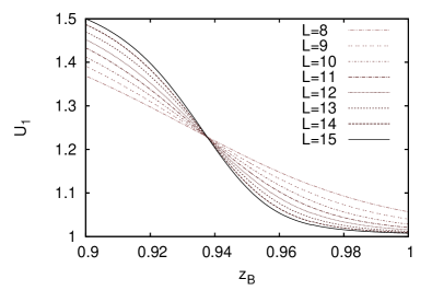
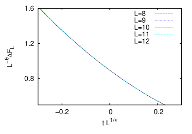
The path facilitates a first test of the scaling of the quenched-averaged barrier , where the sum is over all considered random field samples. For distributions where a barrier cannot be meaningfully defined, such as single or triple peaks, is set to zero. In Fig. 10(a), we show versus for various . Following modified hyperscaling, we expect to scale conform Eq. (39). Hence, plotting versus , , the curves for different should collapse, provided suitable values of , , and are used. This result is shown in Fig. 10(b). Here, was assumed, and by varying and , a data collapse is indeed obtained (the plot uses and ). We have verified that by using , i.e. the value of the pure model, no data collapse is obtained. The estimate of is rather large, but still within the range of values reported in Table 1. Note also that used in Fig. 10(b) agrees with that of the disconnected cumulant intersections, Fig. 6(b).

We now propose one additional method to locate the critical temperature. To this end, recall the FSS expressions and . Since , the ratio becomes -independent at criticality. One can thus locate by plotting versus for various system sizes, and look for intersection points. This approach has the advantage that the critical exponents themselves need not be provided. The connected susceptibility is obtained from the individual distributions using . In Fig. 11(a), we plot versus for various . The data indeed intersect, providing important confirmation that the barrier scales with the same exponent as the connected susceptibility at criticality. For completeness, we show in Fig. 11(b) the disconnected cumulant versus for various (now obtained using the path ). The curves also intersect, and do so remarkably close to the intersections of . Based on Fig. 11, we (VFB) report , where the error reflects the scatter in the various intersection points (here the data of the smallest system was ignored).

We now turn to the distribution , defined as the probability of a particular random field sample yielding a magnetization . At criticality, we anticipate scaling of this distribution, conform Eq. (36). We have explicitly measured by accumulating a histogram of values at using the path . The resulting distributions are shown in Fig. 12. The salient features are a sharp peak, and a long tail extending to lower values. The fact that features a sharp peak is consistent with being close to unity at criticality. Since in the RFIM, the scaling variable is identical to itself, and so the “raw” distributions for different should already overlap with each other. Within numerical precision this is confirmed, but it is clear that the data in Fig. 12 do not allow for any meaningful estimate of .
The point that we wish to make, however, is a different one. The fact that features a long tail means that occasionally a distribution is observed with a significantly lower magnetization. Since the scaling form, Eq. (36), implies that retains its shape irrespective of , the fraction of these distributions does not vanish in the thermodynamic limit. It is conceivable that distributions from the “tail” of are also shaped differently. For instance, consider again the histogram at (Fig. 9(b)). The histograms peak at , so most distributions are bimodal. However, also features a tail, so distributions with profoundly different shapes, although rare, do occur. In particular, the tail in allows for three-peaked distributions to be present (for which ). Indeed, such distributions are observed, and have been interpreted to signify first-order transitions newman , or new phases alvarez . Our point is that the long tail of and its scale invariance at (implied by modified hyperscaling) also allows for the presence of three-peaked distributions (without having to assume a first-order transition, or the emergence of a new phase).
V Widom-Rowlinson model with quenched obstacles
It was argued by de Gennes that a binary mixture undergoing phase separation inside a random network of quenched obstacles belongs to the universality class of the RFIM 39 . The argument is expected to hold when the obstacles display a preferred affinity to one of the phases. In case there is no such preference, the argument does not apply sanctis ; vink_review . Previous simulations 6 have already produced evidence in favor of de Gennes’ argument. To provide further confirmation, in particular to test the scaling of the free energy barrier (Eq. (6)), we consider in this section the Widom-Rowlinson binary mixture (WRM) WidomRowlinson . The model consists of unit diameter spheres, species or , which may overlap freely except for a hard-core repulsion between and particles. The model is investigated in the grand-canonical ensemble, where the relevant thermodynamic parameters are the fugacities, and , of the respective species.
At high fugacities, the WRM can be in two phases: a phase rich in particles (the -phase) when , and a phase rich in particles (the -phase) when . Due to the model’s symmetry under the exchange of and particles, the phase transition occurs at . Hence, in line with the Ising model, a symmetry path for the WRM can be defined as . The transition line ends in an Ising critical point, at fugacity , below which mixed states appear WRCP1 ; WRCP2 . Note that the phase transition in the WRM can also be considered a liquid-gas transition. By integrating out the particles, the WRM maps onto a single component fluid, interacting via a short-ranged attractive potential WidomRowlinson . The fugacity then plays the role of inverse temperature, the -phase corresponds to the liquid (characterized by a high particle density), and the -phase to a gas (low particle density).
V.1 pure mixture

We first consider the pure WRM, i.e. without quenched obstacles. We simulate using cubic boxes with periodic boundary conditions (see Appendix A.5). The analogue of the Ising model OPD is the distribution , defined as the probability for a system of lateral extension to contain particles of species . Since we are ultimately interested in locating the critical point, only OPDs lying on the symmetry path are considered in this section, which leaves as the single free parameter. Note that we could also have defined the OPD as , thereby directly exploiting the symmetry of the WRM. However, most fluids lack such an obvious symmetry, and by using we ensure that our analysis remains generally applicable.
Above the critical fugacity, , is bimodal: the peak at low (high) density corresponds to the gas (liquid) phase. When , the OPD features a single peak, corresponding to a mixed state. The analogue of the magnetization is defined as , which is readily substituted in Eq. (18) to yield the order parameter and susceptibility. Additionally, we define a “generalized” susceptibility orkoulas ; locus
| (44) |
The most straightforward method to locate the critical point is from intersections of the Binder cumulant for different . For the pure WRM, we find that a sharp intersection of can be found easily (Fig. 13). Another method to locate the critical fugacity is via the extrapolation of the finite-size extrema of and . In a finite system of size , reaches a maximum at fugacity , which is shifted from as locus
| (45) |
with the correlation length critical exponent. In addition, reaches a minimum and maximum, at respective fugacities and , which are also shifted according to Eq. (45). Hence, plotting , , and versus , and then linearly extrapolating to , three additional estimates of are obtained. For this extrapolation, hyperscaling is not required, but needs to be provided. In principle, can also be taken as a fit parameter, but this requires data of extremely high quality. For the pure WRM, which belongs to the Ising universality class, is known (cf. Table 1). In Fig. 14, the extrapolation is demonstrated; the resulting estimates of are similar and agree with the cumulant intersections. Combining all results, we obtain , where the error reflects the scatter between the individual estimates. This value is in good agreement with previous results WRCP1 ; WRCP2 .
V.2 mixture with quenched obstacles


We now consider the WRM model with quenched obstacles. We use spherical obstacles, species and , having the same diameter as the (mobile) and particles. The total number of and obstacles equals , rounded up or down at random to the next integer. The obstacles are distributed randomly at the start of the simulation, irrespective of overlap, after which they remain quenched: this defines one disorder realization . Next, and particles are introduced, and grand canonical MC is used to construct for that disorder realization (see Appendix). The -particles (-particles) have a hard-core interaction with -obstacles (-particles) but do not interact with -obstacles (-obstacles). The original motivation for this choice was to restore the symmetry line in the disorder average. However, in what follows, we will use the path , whereby is tuned for each realization of disorder such that is maximized.
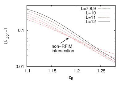
We still need to specify the obstacle concentration . For a noticeable random field effect, the thermal correlation length should be large compared to the typical distance between obstacles. Following the FSS “Ansatz” , this implies . If is too small, crossover scaling is observed (in this case from pure Ising to random field Ising 6 ). From these considerations, choosing a high value of seems optimal. The disadvantage is that also will then be very high, which makes the grand canonical MC approach inefficient due to a high particle density. Clearly, a compromise needs to be made: we use . This value is small compared to typical density of the mobile species, e.g. at criticality in the pure WRM, and certainly is below the percolation threshold; we thus remain in the limit of weak random fields. For the chosen obstacle density, crossover effects are still strong in small systems. This can be inferred from Fig. 15, where the connected cumulant versus for various is plotted. The curves for reveal an intersection point: this would be consistent with a conventional critical point featuring standard hyperscaling. However, for , the intersection has vanished, indicating that the crossover has largely completed. In what follows, we therefore discard the data for in some of the analysis.
Investigations involving disconnected quantities require enormous simulational effort to generate data of sufficient quality (see Fig. 19 in Appendix A.2). For the WRM, an analysis of along the lines of Fig. 11(b) was not feasible. We therefore focus on the free energy barrier. We evaluate the distributions along the path , and for each distribution, we “read-off” the barrier, which is then averaged over the samples to obtain . We first consider the variation of versus for different , i.e. the analogue of Fig. 11(a). This data is shown in Fig. 16; from the intersection we conclude that the critical fugacity is around . To get the critical exponents, we consider the scaling of the free energy barrier. Assuming RFIM universality, the variation of with should follow Eq. (39), where now . In the vicinity of , i.e. as indicated by Fig. 16, we indeed find that a collapse of the curves can be realized for , , and (Fig. 17). As a consistency check, we attempt to obtain from the extrapolation of the extrema of the susceptibilities using Eq. (45). The observables and of the pure model are now replaced by their disorder-averaged counterparts and , and , i.e. the estimate from Fig. 17, is used. The extrapolation works reasonably well (Fig. 18) and for the critical fugacity we obtain the same estimate as before: .
VI Summary
Modified hyperscaling, Eq. (2), which is believed to describe systems belonging to the universality class of the RFIM, gives rise to rather unusual finite size effects at critical points: neither the order parameter distribution, nor the free energy barrier of interface formation, are scale invariant. As a result, “standard” techniques to locate critical points, such as the “cumulant intersection method” 15 , or the Lee-Kosterlitz method lee , break down. However, by carefully considering the consequences of Eq. (2), alternative techniques to derive in random field systems can be derived. In this paper, we have proposed two such techniques. The first is based on the order parameter fluctuations between disorder samples: modified hyperscaling predicts that these are scale invariant at . This property can be used to locate by measuring the disconnected cumulant (Eq. (37)) versus temperature for various system sizes: at , curves for different intersect. Indeed, simulation data of the RFIM confirm the scaling of (Fig. 6(b) and Fig. 11(b)). In contrast to conventional critical points, there is no intersection of the connected cumulant (Eq. (35)) in the RFIM at . However, in small systems, there may be crossover effects. In this case, an apparent intersection in is observed, at , but it vanishes in larger systems; such was the case for the WRM (Fig. 15).
The practical disadvantage of measuring is that many disorder samples must be averaged over if meaningful results are to be obtained. Particularly for more complex systems, such as off-lattice fluids, an economic alternative is to consider the free energy barrier of interface formation. Due to modified hyperscaling, the barrier diverges at , with the violation of hyperscaling exponent. The consequences of this divergence are easily detected in simulations, as was demonstrated for the RFIM (Fig. 10 and Fig. 11(a)), and the WRM (Fig. 16 and Fig. 17). In case of the RFIM, the estimate of obtained from the scaling of the barrier was fully consistent with that obtained from the intersections of (Fig. 11). Our results for the WRM provide further confirmation that fluids with quenched disorder indeed belong to the universality class of the RFIM, consistent with the conjecture of de Gennes 39 .
We have also commented on the variations in shape of the order parameter distribution between samples. There is some question as to whether distributions with three peaks signify first-order transitions newman , or the emergence of new phases alvarez . Our view is that modified hyperscaling also allows for these shape variations. While our data indicate that at , and using the path , the majority of distributions is bimodal, a fraction of distributions with different shape is not ruled out (Fig. 9(b) and Fig. 12).
Finally, we remind the reader that the divergence of the free energy barrier at will also influence the dynamics. Taking the RFIM with single spin-flip dynamics as example, it follows that the largest relaxation time in a finite system at criticality is given by an Arrhenius’ type formula
| (46) |
This is in contrast to the pure model, where the relaxation time (not its logarithm) scales , with the “dynamical critical exponent”. Such a power law for the logarithm of the relaxation time is the hallmark of “activated critical dynamics”. In fact, if we are somewhat above , but the system size is still less than the correlation length, , Eq. (46) still holds! As , the system size in Eq. (46) gets replaced by , and we recover Eq. (4), as proposed by Villain 26 and Fisher 27 . A direct study of the dynamics of a kinetic version of the RFIM would be illuminating, but goes beyond the scope of the present paper.
Acknowledgements.
This work was supported by the Deutsche Forschungsgemeinschaft (Emmy Noether program: VI 483/1-1).References
- (1) Y. Imry and S. K. Ma, Phys. Rev. Lett. 35, 1399 (1975)
- (2) S.F. Edwards and P.W. Anderson, J. Phys. F 5, 965 (1975)
- (3) R.B. Stinchcombe, Dilute Magnetism, in: Phase Transitions and Critical Phenomena, Vol 7, edited by C. Domb and J.L. Lebowitz (Academic Press, London, 1983) p. 151.
- (4) A.P. Young (ed.) Spin Glasses and Random Fields (World Scientific, Singapore, 1998)
- (5) K. Binder and W. Kob, Glassy Materials and Disordered Solids: An Introduction to their Statistical Mechanics (World Scientific, Singapore, 2005)
- (6) R.L.C. Vink, K. Binder and H. Löwen, Phys. Rev. Lett. 97, 230603 (2006); J. Phys.: Condens. Matter 20, 404222 (2008)
- (7) M. E. Fisher, Rev. Mod. Phys. 46, 597 (1974)
- (8) J. Zinn-Justin, Phys. Rep. 344, 159 (2001)
- (9) K. Binder, Rep. Progr. Phys. 60, 487 (1997)
- (10) K. Binder and E. Luijten, Phys. Rep. 344, 179 (2001)
- (11) K. Binder and D. W. Heermann, Monte Carlo Simulation in Statistical Physics. An Introduction, 4th Ed. (Springer, Berlin, 2002)
- (12) M. E. Fisher, in Critical Phenomena, ed. by M.S. Green (Academic Press, London, 1971) p.1.
- (13) V. Privman (ed.) Finite Size Scaling and Numerical Simulation of Statistical Systems (World Scientific, Singapore, 1990)
- (14) K. Binder, Z. Phys. B 43, 119 (1981)
- (15) K. Binder, Phys. Rev. A 25, 1699 (1982)
- (16) K. Binder and D.P. Landau, Phys. Rev. B 30, 1477 (1984)
- (17) A. Aharony and A. B. Harris, Phys. Rev. Lett. 77, 3700 (1996)
- (18) S. Wiseman and E. Domany, Phys. Rev. Lett. 81, 22 (1998); Phys. Rev. E 52, 3469 (1995); Phys. Rev. E 58, 2938 (1998)
- (19) E. Kierlik, P. A. Monson, M. I. Rosinberg, and G. Tarjus, J. Phys.: Condens. Matter 14, 9295 (2002)
- (20) A. Malakis and N. G. Fytas, Phys. Rev. E 73, 016109 (2006)
- (21) P.E. Berche, C. Chatelain, B. Berche and W. Janke, Eur. Phys. J. B 38, 463 (2004)
- (22) J.Z. Imbrie, Phys. Rev. Lett. 53, 1747 (1984)
- (23) H. Rieger, Phys. Rev. B 52, 6659 (1995)
- (24) M. E. J. Newman and G. T. Barkema, Phys. Rev. E 53, 393 (1996)
- (25) J. Villain, J. Phys. (France) 46, 1843 (1985)
- (26) D. S. Fisher, Phys. Rev. Lett. 56, 416 (1986)
- (27) T. Nattermann, Theory of the Random Field Ising Model, in: Spin Glasses and Random Fields, edited by A. P. Young (World Scientific, Singapore, 1998), p. 277; see also arXiv:cond-mat/9705295
- (28) M. Schwartz, J. Phys. C: Solid State Phys. 18, 135 (1985)
- (29) M. Schwartz, M. Gofman, and T. Nattermann, Physica A 178, 6 (1991)
- (30) M. Gofman, J. Adler, A. Aharony, A.B. Harris, and M. Schwartz, Phys. Rev. Lett. 71, 1569 (1993)
- (31) P.C. Hohenberg and B.I. Halperin, Rev. Mod. Phys. 49, 435 (1977)
- (32) A.P. Young and M. Nauenberg, Phys. Rev. Lett. 54, 2429 (1985)
- (33) E. Eichhorn and K. Binder, Europhys. Lett. 30, 331 (1995); J. Phys.: Condens. Matter 8, 5209 (1996)
- (34) H. E. Stanley, Introduction to Phase Transitions and Critical Phenomena (Oxford University Press, Oxford, 1971)
- (35) N. G. Fytas, A. Malakis, and K. Eftaxias, J. Stat. Mech. 2008, P03015 (2008)
- (36) G. Orkoulas, A. Z. Panagiotopoulos, and M. E. Fisher, Phys. Rev. E 61, 5930 (2000)
- (37) A. K. Hartmann and U. Nowak, Eur. Phys. J. B 7, 105 (1999)
- (38) M. S. Cao and J. Machta, Phys. Rev. B 48, 3177 (1993)
- (39) C. Borgs and R. Kotecký, J. Stat. Phys. 61, 79 (1990)
- (40) N. B. Wilding and A. D. Bruce, J. Phys. Condens. Matter. 4, 3087 (1992)
- (41) E. Luijten, M. E. Fisher, and A. Panagiotopoulos, Phys. Rev. Lett. 88, 185701 (2002)
- (42) B. Grossmann and M. L. Laursen, Nucl. Phys. B, 408 637 (1993)
- (43) J. Lee and J. M. Kosterlitz, Phys. Rev. Lett. 65, 137 (1990)
- (44) C. Borgs and S. Kappler, Phys. Lett. A 171, 37 (1992)
- (45) G. Orkoulas, M. E. Fisher, and A. Z. Panagiotopoulos, Phys. Rev. E 63, 051507 (2001)
- (46) J. Machta, M. E. J. Newman, and L. B. Chayes, Phys. Rev. E 62, 8782 (2000)
- (47) M. Álvarez, D. Levesque, and J.-J. Weis, Phys. Rev. E 60, 5495 (1999)
- (48) P. G. de Gennes, J. Phys. Chem. 88, 6469 (1984)
- (49) P. G. De Sanctis Lucentini and G. Pellicane, Phys. Rev. Lett. 101, 246101 (2008)
- (50) R.L.C. Vink, Soft Matter 5, 4388 (2009)
- (51) B. Widom, J. S. Rowlinson, J. Chem. Phys. 52, 1670 (1970).
- (52) G. Johnson, H. Gould, J. Machta, L.K. Chayes, Phys. Rev. Lett. 79, 2612 (1997).
- (53) R.L.C. Vink, J. Chem. Phys. 124, 094502 (2006)
- (54) F. Wang and D. P. Landau, Phys. Rev. Lett. 86, 2050 (2001)
- (55) A. M. Ferrenberg and R. H. Swendsen, Phys. Rev. Lett. 61, 2635 (1988)
- (56) P. Virnau and M. Müller, J. Chem. Phys. 120, 10925 (2004)
*
Appendix A Simulation Details
A.1 Wang-Landau sampling
The simulations of the Ising and RFIM were performed using Wang-Landau (WL) sampling wls . The OPD is written as
| (47) |
with the total instantaneous magnetization, and some generalized density of states (DOS). Note that the DOS depends on system size , temperature , and random field sample , but not on the external field (for the pure Ising model, there is no dependence on either, of course). At the start of each simulation, we generate a sample of random fields . We then perform single spin-flips, whereby one of the spins is chosen at random, and its orientation reversed. Let the total magnetization and energy at the start of each spin-flip be given by and , respectively, and afterward by and ; each spin-flip is then accepted with probability
| (48) |
Note that the energy above refers to the configurational part of the Hamiltonian only, i.e. the nearest-neighbor interaction and the coupling to the random field, but not the coupling to the external field.
The DOS is a-priori unknown, and is initially set to unity . After each attempted spin-flip, one “updates” the DOS , with the magnetization of the system after the attempted spin-flip. The update is performed irrespective of whether the spin-flip was accepted; the initial modification factor . We also update a histogram , counting how often a state with magnetization was visited. This procedure is repeated until has become sufficiently flat, which completes one WL iteration. We use the criterion , with and the smallest and largest entries in , respectively. After the first WL iteration, the modification factor is reduced , the histogram is reset to zero, and the procedure is repeated. WL iterations are continued until has become small such that changes to the DOS become negligible. For each DOS, we typically performed 150–250 WL iterations. Once the DOS is known, the OPD can be calculated for arbitrary values of using Eq. (47).
A.2 Importance of disorder averaging

To accurately determine disorder averages, the OPD is measured times. In particular disconnected quantities require a large number of disorder samples if meaningful results in the critical regime are to be obtained. Fig. 19 shows a typical “running average” of and versus . While saturates to a plateau already after 1000 samples, the convergence of is noticeably slower. The data of Fig. 19 indicate that should exceed several thousands at least. Away from the critical point, is no longer divergent, and here we expect that lower values of will also suffice.
A.3 Histogram reweighting in temperature
A key ingredient in this work is the use of histogram reweighting in the temperature-like variable. We perform our simulations at only a few distinct temperatures, and extrapolate to other values using histogram reweighting hrw . This requires that the joint two-dimensional probability distribution , of the magnetization and energy , is known. Again, as in Eq. (48), refers to the configurational part of the Hamiltonian only. If is measured for and , it can be extrapolated to other values using a generalization of Eq. (47)
| (49) |
with and . The practical problem is that two-dimensional histograms require considerable disk space, which in the case of quenched disorder is multiplied by a factor . Fortunately, an excellent approximation can be used to drastically reduce storage requirements 6 . Without loss of generality, we write
| (50) |
where is the probability distribution of the energy measured at states with the same magnetization . The approximation is to assume that is Gaussian, and so is fully specified by its first two moments. For each random field sample, the two-dimensional histogram of Eq. (50) then requires only to be stored, plus the “functions” and .
A.4 Alternative method to measure the barrier

It is also possible to measure the quenched-averaged free energy barrier using the same external field for all samples. To be concrete, consider the OPD of the RFIM obtained at fixed , i.e. the symmetry path, with total magnetization and . We define the quenched-averaged free energy difference between “adjacent” states as
| (51) |
which can be used to construct a total free energy by means of recursion
| (52) |
Fig. 20(a) shows the typical shape of the free energy obtained in this way for the RFIM. The distribution is bimodal, and a free energy barrier can be meaningfully “read-off”. As it turns out, this barrier is very similar to that obtained by averaging over individual samples, i.e. as was done in Fig. 10(a) using the path ; a comparison is provided in Fig. 20(b). In fact, if one uses to perform the scaling analysis of Fig. 10(b), excellent data collapses are also realized.
An analysis in terms of is numerically convenient because extrapolations in the field variable can be performed after the quenched average has been taken
| (53) |
This is particularly useful for fluids, where the critical field (chemical potential) is generally not known beforehand. However, it is not obvious what the peak positions and widths in correspond to. Based on our previous work 6 , cumulants of do intersect at , but (in hindsight) we believe it is safer to perform the cumulant analysis using the individual OPDs (as was done in this work).
A.5 Simulating the Widom-Rowlinson model
We measure using grand canonical MC and successive umbrella sampling (SUS) SUS . The simulations are performed in a periodic 3D cube of volume . At the start of each simulation, a disorder realization is generated by distributing the obstacles and randomly in the cube, i.e. the obstacles are allowed to overlap. We then perform grand canonical MC moves consisting of the insertion and removal of single and particles. In SUS, the full density range of interest is split into overlapping windows . In the first window, is allowed to fluctuate between 0 and 1, in the second window between 1 and 2, or, more generally, in the -th window . There is no restriction on the number of particles: thus fluctuates freely in each window.
For the -particles are an ideal gas in the volume allowed by the quenched -particles so an initial state for is easily constructed: we draw a number from a Poissonian distribution , and randomly insert this number of -particles into the system, discarding all -particles that overlap with -obstacles. As starting state for the subsequent windows , we take the last state of the window preceding it, and equilibrate this state briefly for MC steps within the bounds of the new window. This works well in practice because the windows are small.
The production run of each window is performed using MC steps. Each step first selects a species, , with equal probability. Then, with equal probability, the insertion or removal of a particle of species is attempted. In case of removal, a particle of species is picked at random and removed from the system; the resulting new state is accepted with probability
| (54) |
The factor is one when ; for , it will be specified later. In case insertion is chosen, a new particle of species is placed at a random location; the resulting new state is accepted with probability
| (55) |
States with hard-core overlaps and states where is outside the window bounds are always rejected, irrespective of the accept probabilities.
While simulating in window , we keep track of two counters, and . These count, respectively, how often the state with and was visited. From these counters, we construct the relative probability of these states via
| (56) |
Having at hand this ratio for all windows , the full distribution is constructed recursively
| (57) |
where the proportionality constant follows from normalization. Note that above is, of course, fully equivalent to the OPD that we wish to find.
We now specify the factor for moves involving -particles. Assuming a constant number of steps per window, Eq. (56) suggests that optimal results are obtained when is chosen such that and are roughly equal, i.e. , which is the sought-for result itself. For the first window we use the pure model’s optimal weight, which can be calculated analytically. For the subsequent windows, we linearly extrapolate to calculate to be used in that window. In practice, this choice is already quite good, and the counts in the upper and lower bin consistently lie within of each other.
In view of the huge amount of disorder realizations required, a mechanism that allows for histogram reweighting of results obtained at to nearby parameters is indispensable. To facilitate this reweighting, the joint probability distribution is stored in compact form as described in Appendix A.3; the results of that section trivially transfer to the WRM if one identifies and . For the WRM with quenched disorder, the range in over which one can reliably extrapolate is too small to cover the full region of interest. In particular, simulation data obtained at the fugacity of the susceptibility maximum could not be extrapolated to the critical fugacity . We therefore created two data sets per system size. One set with disorder realizations at used for locating the extrema of and (Fig. 18) and one set with realizations around , which is close to , for investigating the free energy barrier (Figs. 16 and 17).