Note on Non-Gaussianities in Two-field Inflation

Abstract

Two-field slow-roll inflation is the most conservative modification of a single-field model. The main motivations to study it are its entropic mode and non-Gaussianity. Several years ago, for a two-field model with additive separable potentials, Vernizzi and Wands invented an analytic method to estimate its non-Gaussianities. Later on, Choi et al. applied this method to the model with multiplicative separable potentials. In this note, we design a larger class of models whose non-Gaussianity can be estimated by the same method. Under some simplistic assumptions, roughly these models are unlikely able to generate a large non-Gaussianity. We look over some specific models of this class by scanning the full parameter space, but still no large non-Gaussianity appears in the slow-roll region. These models and scanning techniques would be useful for future model hunt if observational evidence shows up for two-field inflation.

I Introduction

Cosmic inflation Guth:1980zm is a great idea to solve some cosmological problems and to predict the fine fluctuations of cosmic microwave background (CMB). Hitherto the surviving and most economical model of inflation involves a single scalar field slowly rolling down its effective potential Linde:1981mu ; Albrecht:1982wi , with a canonical kinetic term and minimally coupled to the Einstein gravity. We will call it the simplest single-field inflation, although there is still freedom to design its exact potential. The single-field inflation passed the latest observational test Komatsu:2010fb successfully, even with the simplest quadratic potential.

Nevertheless there are perpetual attempts to modify the simplest single-field inflation. Some of them are motivated by incorporating inflation model into certain theoretical frameworks, such as the standard model of particle physics Bezrukov:2007ep ; DeSimone:2008ei or string theory Kachru:2003sx . Some others put their stake on signatures that cannot appear in the simplest single-field model, such as a large deviation from the Gaussian distribution in the CMB temperature fluctuations.

Among these modifications, the two-field slow-roll inflation is the most conservative one, at least in my personal point of view. It introduces another scalar field rather than a non-conventional Lagrangian such as non-canonical kinetic terms or modifications of gravity. It also retains the slow-roll condition, which makes the model simple and consistent with the observed CMB power spectrum. If both conventional Lagrangian and non-conventional Lagrangian are adaptable to the observational data, then the model with conventional Lagrangian would be more acceptable, unless there are better and solid theoretical motivations for non-conventional Lagrangian.

On the observational side, two new features arise in two-field model. First, the model is able to leave a residual entropic perturbation between the fluctuations of dark matter and CMB GarciaBellido:1995qq ; Byrnes:2006fr . Second, in a simple model with quadratic potential, numerical computations Rigopoulos:2005us ; Vernizzi:2006ve found that the non-Gaussianity can be temporarily large at the turn of inflation trajectory in field space. Longer-lived large non-Gaussianities were discovered recently by Byrnes:2008wi ; Byrnes:2008zy ; Byrnes:2009qy in many other two-field models.

Compared with the simplest one-field inflation, the field space becomes two-dimensional in a two-field model. When the inflation trajectory is curved in field space, the entropic perturbation will be coupled to the adiabatic perturbation. So there are more uncertainties in calculation of cosmological observables, such as power spectra of CMB and their indices. It would be more complicated to honestly compute the bispectra and non-linear parameters, which reflect the non-Gaussianity of the primordial fluctuations.

Fortunately, based on the extended $\delta N$-formalism Lyth:2005fi , Vernizzi and Wands Vernizzi:2006ve invented an analytic method to estimate such non-Gaussianities. They demonstrated the power of this method in a two-field model with additive separable potentials. This method was later applied by Choi et al. Choi:2007su to a model with multiplicative separable potentials.

Encouraged by the method of Vernizzi and Wands, we tried to improve it for the two-field slow-roll model with generic potentials but failed. Finally, we only designed a larger class of models whose non-Gaussianity can be estimated by this method. It is a class of models whose potential take the form $W(w)$ with $w=U(\varphi)+V(\chi)$ or $w=U(\varphi)V(\chi)$. Here $W(w)$, $U(\varphi)$ and $V(\chi)$ are arbitrary functions of the indicated variables as long as the slow-roll condition is satisfied. Scalar fields $\varphi$ and $\chi$ are inflatons.

The outline of this paper is as follows. In our convention of notations, we will prepare some well-known but necessary knowledge in section II concisely. In section III, we will present the exact form of our models, whose non-linear parameters will be worked out in sections IV and V. Some specific examples are investigated in section VI. We summarize the main results of this paper in the final section.

This is a note concerning references Vernizzi:2006ve ; Choi:2007su . Some of our techniques stem from these references or slightly generalize theirs. Sometimes we employ the techniques with few explanation if the mathematical development is smooth. To better understand them, the readers are strongly recommended to review the relevant parts of Vernizzi:2006ve ; Choi:2007su .

II Non-Gaussianities in Two-field Inflation

We are interested in inflation models described by the following action DiMarco:2005nq ; Choi:2007su

$$S=\int d^{4}x\sqrt{-g}\left[\frac{1}{2}M_{p}^{2}R-\frac{1}{2}g^{\mu\nu}\partial_{\mu}\varphi\partial_{\nu}\varphi-\frac{1}{2}e^{2b(\varphi)}g^{\mu\nu}\partial_{\mu}\chi\partial_{\nu}\chi-W(\varphi,\chi)\right].$$ (1)

Because of the appearance of $b(\varphi)$, the field $\chi$ has a non-standard kinetic term. Following the notation of slow-roll parameters defined in GarciaBellido:1995qq ; DiMarco:2005nq

$$\epsilon_{\varphi}=\frac{M_{p}^{2}}{2}\left(\frac{W_{,\varphi}}{W}\right)^{2},\leavevmode\nobreak\ \leavevmode\nobreak\ \leavevmode\nobreak\ \leavevmode\nobreak\ \epsilon_{\chi}=\frac{M_{p}^{2}}{2}\left(\frac{W_{,\chi}}{W}\right)^{2}e^{-2b},\leavevmode\nobreak\ \leavevmode\nobreak\ \leavevmode\nobreak\ \leavevmode\nobreak\ \epsilon_{b}=8M_{p}^{2}b_{,\varphi}^{2},$$

$$\eta_{\varphi\varphi}=\frac{M_{p}^{2}W_{,\varphi\varphi}}{W},\leavevmode\nobreak\ \leavevmode\nobreak\ \leavevmode\nobreak\ \leavevmode\nobreak\ \eta_{\varphi\chi}=\frac{M_{p}^{2}W_{,\varphi\chi}}{W}e^{-b},\leavevmode\nobreak\ \leavevmode\nobreak\ \leavevmode\nobreak\ \leavevmode\nobreak\ \eta_{\chi\chi}=\frac{M_{p}^{2}W_{,\chi\chi}}{W}e^{-2b},$$ (2)

the slow-roll condition can be expressed as $\epsilon_{i}\ll 1$, $\epsilon_{b}\ll 1$, $|\eta_{ij}|\ll 1$ with $i,j=\varphi,\chi$.

As an aside, we mention that model (1) is equivalent to the $f(\chi,R)$ generalized gravity Hwang:2005hb ; Ji:2009yw when $b=-\varphi/(\sqrt{6}M_{p})$. But then we find $\epsilon_{b}=4/3$, which violates the the slow-roll condition. This is a pitfall in treating generalized gravity as a two-field model. This pitfall can be circumvented by the scheme in Ji:2009yw .

Under the slow-roll condition, the background equations of motion are very simple

$$3H\dot{\varphi}+W_{,\varphi}=0,\leavevmode\nobreak\ \leavevmode\nobreak\ \leavevmode\nobreak\ \leavevmode\nobreak\ 3He^{2b}\dot{\chi}+W_{,\chi}=0,\leavevmode\nobreak\ \leavevmode\nobreak\ \leavevmode\nobreak\ \leavevmode\nobreak\ 3M_{p}^{2}H^{2}=W.$$ (3)

Using them one may directly demonstrate

$$\epsilon=-\frac{\dot{H}}{H^{2}}=\epsilon_{\varphi}+\epsilon_{\chi}.$$ (4)

Observationally, the most promising probe of primordial non-Gaussianities comes from the bispectrum of CMB fluctuations, which is characterized by the non-linear parameter $f_{\mathrm{NL}}(\mathbf{k}_{1},\mathbf{k}_{2},\mathbf{k}_{3})$. If $|f_{\mathrm{NL}}|\gtrsim 10$, it would be detectable by ongoing or planned satellite experiments planck ; cmbpol .

It has been shown in Seery:2005gb ; Vernizzi:2006ve ; Choi:2007su that the non-linear parameter in two-field inflation models can be separated into a momentum dependent term and a momentum independent term

$$-\frac{6}{5}f_{\mathrm{NL}}(\mathbf{k}_{1},\mathbf{k}_{2},\mathbf{k}_{3})=-\frac{6}{5}f_{\mathrm{NL}}^{(3)}(\mathbf{k}_{1},\mathbf{k}_{2},\mathbf{k}_{3})-\frac{6}{5}f_{\mathrm{NL}}^{(4)}$$ (5)

It is also proved in Vernizzi:2006ve ; Choi:2007su that the first term is always suppressed by the tensor-to-scalar ratio, leading to $|f_{\mathrm{NL}}^{(3)}|\ll 1$. Hence this term is negligible in observation. For action (1), the second term

$$-\frac{6}{5}f_{\mathrm{NL}}^{(4)}=\frac{N_{,\varphi_{*}}^{2}N_{,\varphi_{*}\varphi_{*}}+2e^{-2b_{*}}N_{,\varphi_{*}}N_{,\chi_{*}}N_{,\varphi_{*}\chi_{*}}+e^{-4b_{*}}N_{,\chi_{*}}^{2}N_{,\chi_{*}\chi_{*}}}{\left(N_{,\varphi_{*}}^{2}+e^{-2b_{*}}N_{,\chi_{*}}^{2}\right)^{2}}$$ (6)

may be large and deserves a closer look. Here $N=\int_{*}^{c}Hdt$ is the $e$-folding number from the initial flat hypersurface $t=t_{*}$ to the final comoving hypersurface $t=t_{c}$. To evaluate (6), we will work out the derivatives of $N$ with respect to $\varphi_{*}$ and $\chi_{*}$ in the next section, focusing on a class of analytically solvable models.

III Hunting for Analytically Solvable Models

Making use of equations (3), the $e$-folding number can be cast as

$$N = \int_{*}^{c}Hdt$$ (7)

$$= -\int_{*}^{c}\frac{(W-Q)\dot{\varphi}}{M_{p}^{2}W_{,\varphi}}dt-\int_{*}^{c}\frac{Q(\varphi,\chi)\dot{\chi}}{M_{p}^{2}W_{,\chi}}e^{2b(\varphi)}dt$$

$$= -\int_{*}^{c}\frac{W-Q}{M_{p}^{2}W_{,\varphi}}d\varphi-\int_{*}^{c}\frac{Qe^{2b}}{M_{p}^{2}W_{,\chi}}d\chi.$$

Hence $Q(\varphi,\chi)$ is an arbitrary function of $\varphi$ and $\chi$ in principle, because $\dot{\varphi}/W_{,\varphi}=e^{2b}\dot{\chi}/W_{,\chi}=-1/(3H)$ along any classical trajectory under the slow-roll condition. However, for a given $W$, we have to choose a suitable form of $Q$ so that the integrations defined by $\mathcal{Q}$ in (III) can be performed. Later on we will fix $Q$ to meet the ansatz (20) for simplicity. But for the moment let us leave it as an arbitrary function of $\varphi$ and $\chi$. It is straightforward to obtain the first order partial derivatives

$$\frac{\partial N}{\partial\varphi_{*}} = \frac{W^{*}-Q^{*}}{M_{p}^{2}W^{*}_{,\varphi}}-\frac{W^{c}-Q^{c}}{M_{p}^{2}W^{c}_{,\varphi}}\frac{\partial\varphi_{c}}{\partial\varphi_{*}}-\int_{*}^{c}\left(\frac{W-Q}{M_{p}^{2}W_{,\varphi}}\right)_{,\chi}\frac{\partial\chi}{\partial\varphi_{*}}d\varphi$$

$$-\frac{Q^{c}e^{2b_{c}}}{M_{p}^{2}W^{c}_{,\chi}}\frac{\partial\chi_{c}}{\partial\varphi_{*}}-\int_{*}^{c}\left(\frac{Qe^{2b}}{M_{p}^{2}W_{,\chi}}\right)_{,\varphi}\frac{\partial\varphi}{\partial\varphi_{*}}d\chi,$$

$$\frac{\partial N}{\partial\chi_{*}} = -\frac{W^{c}-Q^{c}}{M_{p}^{2}W^{c}_{,\varphi}}\frac{\partial\varphi_{c}}{\partial\chi_{*}}-\int_{*}^{c}\left(\frac{W-Q}{M_{p}^{2}W_{,\varphi}}\right)_{,\chi}\frac{\partial\chi}{\partial\chi_{*}}d\varphi$$ (8)

$$+\frac{Q^{*}e^{2b_{*}}}{M_{p}^{2}W^{*}_{,\chi}}-\frac{Q^{c}e^{2b_{c}}}{M_{p}^{2}W^{c}_{,\chi}}\frac{\partial\chi_{c}}{\partial\chi_{*}}-\int_{*}^{c}\left(\frac{Qe^{2b}}{M_{p}^{2}W_{,\chi}}\right)_{,\varphi}\frac{\partial\varphi}{\partial\chi_{*}}d\chi.$$

Akin to Vernizzi:2006ve ; Choi:2007su , we define an integral of motion $C$ along the trajectory of inflation

$$C=\int\frac{Wf(\varphi,\chi)}{M_{p}^{2}W_{,\varphi}}d\varphi-\int\frac{We^{2b}f}{M_{p}^{2}W_{,\chi}}d\chi,$$ (9)

Here the explicit form of $f(\varphi,\chi)$ is determined by scalar potential $W(\varphi,\chi)$. We will give the expression of $f$ for some types of potential in this section. If we fix the limits of integration to run from $t_{*}$ to $t_{c}$, then due to the background equations (3),

$$\left.C\right|_{*}^{c}=\int_{*}^{c}\frac{Wf}{3M_{p}^{2}H}\left(\frac{\dot{\varphi}}{W_{,\varphi}}-\frac{e^{2b}\dot{\chi}}{W_{,\chi}}\right)dt=0$$ (10)

along classical trajectories under the slow-roll approximation. So the constant $C$ parameterizes the motion off classical trajectories. In order to know $\partial\varphi_{c}/\partial\varphi_{*}$, $\partial\chi_{c}/\partial\varphi_{*}$, $\partial\varphi_{c}/\partial\chi_{*}$, $\partial\chi_{c}/\partial\chi_{*}$ in (III), we should calculate the first order derivatives of $C$ on the initial flat hypersurface $t=t_{*}$,

$$\frac{\partial C}{\partial\varphi_{*}} = \frac{W^{*}f^{*}}{M_{p}^{2}W^{*}_{,\varphi}}+\int^{*}\left(\frac{Wf}{M_{p}^{2}W_{,\varphi}}\right)_{,\chi}\frac{\partial\chi}{\partial\varphi_{*}}d\varphi-\int^{*}\left(\frac{We^{2b}f}{M_{p}^{2}W_{,\chi}}\right)_{,\varphi}\frac{\partial\varphi}{\partial\varphi_{*}}d\chi,$$

$$\frac{\partial C}{\partial\chi_{*}} = \int^{*}\left(\frac{Wf}{M_{p}^{2}W_{,\varphi}}\right)_{,\chi}\frac{\partial\chi}{\partial\chi_{*}}d\varphi-\frac{W^{*}e^{2b_{*}}f^{*}}{M_{p}^{2}W^{*}_{,\chi}}-\int^{*}\left(\frac{We^{2b}f}{M_{p}^{2}W_{,\chi}}\right)_{,\varphi}\frac{\partial\varphi}{\partial\chi_{*}}d\chi.$$ (11)

Differentiating (9) with respect to $C$, it gives

$$1=\frac{Wf}{M_{p}^{2}W_{,\varphi}}\frac{d\varphi}{dC}+\int\left(\frac{Wf}{M_{p}^{2}W_{,\varphi}}\right)_{,\chi}\frac{d\chi}{dC}d\varphi-\frac{We^{2b}f}{M_{p}^{2}W_{,\chi}}\frac{d\chi}{dC}-\int\left(\frac{We^{2b}f}{M_{p}^{2}W_{,\chi}}\right)_{,\varphi}\frac{d\varphi}{dC}d\chi.$$ (12)

On large scales, the comoving hypersurface $t=t_{c}$ coincides with the uniform density hypersurface. This implies under the slow-roll condition

$$W(\varphi_{c},\chi_{c})=\mathrm{const.},$$ (13)

whose differentiation with respect to $C$ is

$$W^{c}_{,\varphi}\frac{d\varphi_{c}}{dC}+W^{c}_{,\chi}\frac{d\chi_{c}}{dC}=0.$$ (14)

Combined with (12) on the final comoving surface $t=t_{c}$, it could give the solution for $d\varphi_{c}/dC$ and $d\chi_{c}/dC$. This is in general difficult analytically. To overcome the difficulty, we introduce an ansatz:

$$\left(\frac{Wf}{M_{p}^{2}W_{,\varphi}}\right)_{,\chi}=\left(\frac{We^{2b}f}{M_{p}^{2}W_{,\chi}}\right)_{,\varphi}=0.$$ (15)

Although we are free to design the function $f(\varphi,\chi)$, the above condition is not always satisfiable. We have hunted for analytical models meeting this condition, and found it is achievable if $W=W(w)$ with $w=U(\varphi)+V(\chi)$ or $w=U(\varphi)V(\chi)$. Here $W(w)$, $U(\varphi)$ and $V(\chi)$ are arbitrary functions of the indicated variables as long as the slow-roll condition is satisfied. In this paper, we will pay attention to this situation. But it is never excluded that there might be other situations in which $d\varphi_{c}/dC$ and $d\chi_{c}/dC$ are solvable from (12) and (14), even if ansatz (15) is violated.

Ansatz (15) simplifies our discussion significantly. Once it holds, equations (12) and (14) lead to

$$\frac{d\varphi_{c}}{dC} = \frac{2W^{c}}{W^{c}_{,\varphi}f^{c}}\frac{\epsilon^{c}_{\varphi}\epsilon^{c}_{\chi}}{\epsilon^{c}},$$

$$\frac{d\chi_{c}}{dC} = -\frac{2W^{c}}{W^{c}_{,\chi}f^{c}}\frac{\epsilon^{c}_{\varphi}\epsilon^{c}_{\chi}}{\epsilon^{c}},$$ (16)

while (III) is reduced as

$$\frac{\partial C}{\partial\varphi_{*}} = \frac{W^{*}f^{*}}{M_{p}^{2}W^{*}_{,\varphi}},$$

$$\frac{\partial C}{\partial\chi_{*}} = -\frac{W^{*}e^{2b_{*}}f^{*}}{M_{p}^{2}W^{*}_{,\chi}}.$$ (17)

As a result, the partial derivatives of $N$ take the form

$$N_{,\varphi_{*}} = \frac{W^{*}-Q^{*}}{M_{p}^{2}W^{*}_{,\varphi}}+(Z^{c}-\mathcal{Q})\frac{\partial C}{\partial\varphi_{*}},$$

$$N_{,\chi_{*}} = \frac{Q^{*}e^{2b_{*}}}{M_{p}^{2}W^{*}_{,\chi}}+(Z^{c}-\mathcal{Q})\frac{\partial C}{\partial\chi_{*}},$$

$$N_{,\varphi_{*}\varphi_{*}} = \left(\frac{W^{*}-Q^{*}}{M_{p}^{2}W^{*}_{,\varphi}}\right)_{,\varphi_{*}}+\left(\frac{\partial Z^{c}}{\partial\varphi_{*}}-\frac{\partial\mathcal{Q}}{\partial\varphi_{*}}\right)\frac{\partial C}{\partial\varphi_{*}}+(Z^{c}-\mathcal{Q})\frac{\partial^{2}C}{\partial\varphi_{*}^{2}},$$

$$N_{,\varphi_{*}\chi_{*}} = \left(\frac{W^{*}-Q^{*}}{M_{p}^{2}W^{*}_{,\varphi}}\right)_{,\chi_{*}}+\left(\frac{\partial Z^{c}}{\partial\chi_{*}}-\frac{\partial\mathcal{Q}}{\partial\chi_{*}}\right)\frac{\partial C}{\partial\varphi_{*}}+(Z^{c}-\mathcal{Q})\frac{\partial^{2}C}{\partial\varphi_{*}\partial\chi_{*}},$$

$$N_{,\chi_{*}\chi_{*}} = \left(\frac{Q^{*}e^{2b_{*}}}{M_{p}^{2}W^{*}_{,\chi}}\right)_{,\chi_{*}}+\left(\frac{\partial Z^{c}}{\partial\chi_{*}}-\frac{\partial\mathcal{Q}}{\partial\chi_{*}}\right)\frac{\partial C}{\partial\chi_{*}}+(Z^{c}-\mathcal{Q})\frac{\partial^{2}C}{\partial\chi_{*}^{2}}.$$ (18)

In these equations, we have adopted the notations

$$Z^{c} = \frac{Q^{c}\epsilon^{c}_{\varphi}-(W^{c}-Q^{c})\epsilon^{c}_{\chi}}{W^{c}f^{c}\epsilon^{c}},$$

$$\mathcal{Q} = \int_{*}^{c}\left(\frac{W-Q}{M_{p}^{2}W_{,\varphi}}\right)_{,\chi}\frac{d\chi}{dC}d\varphi+\int_{*}^{c}\left(\frac{Qe^{2b}}{M_{p}^{2}W_{,\chi}}\right)_{,\varphi}\frac{d\varphi}{dC}d\chi,$$

$$\frac{\partial Z^{c}}{\partial\varphi_{*}} = Z^{c}_{,\varphi}\frac{d\varphi_{c}}{dC}\frac{\partial C}{\partial\varphi_{*}}+Z^{c}_{,\chi}\frac{d\chi_{c}}{dC}\frac{\partial C}{\partial\varphi_{*}},$$

$$\frac{\partial\mathcal{Q}}{\partial\varphi_{*}} = \left(\frac{W^{c}-Q^{c}}{M_{p}^{2}W^{c}_{,\varphi}}\right)_{,\chi_{c}}\frac{d\chi_{c}}{dC}\frac{\partial\varphi_{c}}{\partial\varphi_{*}}-\left(\frac{W^{*}-Q^{*}}{M_{p}^{2}W^{*}_{,\varphi}}\right)_{,\chi_{*}}\frac{d\chi_{*}}{dC}$$ (19)

$$+\frac{\partial C}{\partial\varphi_{*}}\int_{*}^{c}\left(\frac{W-Q}{M_{p}^{2}W_{,\varphi}}\right)_{,\chi\chi}\left(\frac{d\chi}{dC}\right)^{2}d\varphi+\frac{\partial C}{\partial\varphi_{*}}\int_{*}^{c}\left(\frac{W-Q}{M_{p}^{2}W_{,\varphi}}\right)_{,\chi}\frac{d^{2}\chi}{dC^{2}}d\varphi$$

$$+\left(\frac{Q^{c}e^{2b_{c}}}{M_{p}^{2}W^{c}_{,\chi}}\right)_{,\varphi_{c}}\frac{d\varphi_{c}}{dC}\frac{\partial\chi_{c}}{\partial\varphi_{*}}+\frac{\partial C}{\partial\varphi_{*}}\int_{*}^{c}\left(\frac{Qe^{2b}}{M_{p}^{2}W_{,\chi}}\right)_{,\varphi\varphi}\left(\frac{d\varphi}{dC}\right)^{2}d\chi$$

$$+\frac{\partial C}{\partial\varphi_{*}}\int_{*}^{c}\left(\frac{Qe^{2b}}{M_{p}^{2}W_{,\chi}}\right)_{,\varphi}\frac{d^{2}\varphi}{dC^{2}}d\chi.$$

In the above, the expression of $\mathcal{Q}$ and its derivatives involve nuisance integrals. To further simplify our study, we utilize one more ansatz

$$\left(\frac{W-Q}{M_{p}^{2}W_{,\varphi}}\right)_{,\chi}=\left(\frac{Qe^{2b}}{M_{p}^{2}W_{,\chi}}\right)_{,\varphi}=0.$$ (20)

In favor of this ansatz, we have $\mathcal{Q}=0$ and so do its derivatives.

As was mentioned, ansatz (15) can be satisfied by special forms of potential $W(\varphi,\chi)$. Now ansatz (20) further constrains the form of $W(\varphi,\chi)$ and $b(\varphi)$. Let us discuss it in details case by case.

III.1 Case I: $W=W(w)$, $w=U(\varphi)+V(\chi)$

For this class of models, according to (15), we set

$$f=\frac{W_{,w}}{We^{2b}},$$ (21)

while condition (20) is met by

$$b=0,\leavevmode\nobreak\ \leavevmode\nobreak\ \leavevmode\nobreak\ \leavevmode\nobreak\ W=\lambda w^{\alpha},\leavevmode\nobreak\ \leavevmode\nobreak\ \leavevmode\nobreak\ \leavevmode\nobreak\ Q=\lambda Vw^{\alpha-1}$$ (22)

or

$$b=-\frac{1}{2}\nu U,\leavevmode\nobreak\ \leavevmode\nobreak\ \leavevmode\nobreak\ \leavevmode\nobreak\ \frac{d\ln W}{dw}=\frac{1}{p+qe^{\nu w}},\leavevmode\nobreak\ \leavevmode\nobreak\ \leavevmode\nobreak\ \leavevmode\nobreak\ Q=qe^{\nu w}W_{,w}.$$ (23)

Hereafter, as free parameters in our models, $\lambda$, $\alpha$, $\beta$, $\nu$, $p$ and $q$ are arbitrary real constants. The normalization of $e^{2b}$ is fixed for simplicity. This is always realizable by rescaling the field $\chi$.

Taking $\alpha=1$, model (22) recovers the well-studied sum potential Polarski:1992dq ; Langlois:1999dw ; Vernizzi:2006ve , to which we will return in subsection VI.1. In subsection VI.4, we will study a specific example of non-separable potential that corresponds to $\alpha=2$ in (22).

As will be discussed in subsection III.3, there is an equivalence relation between case I in this subsection and case II in the next subsection. Models in class I can be transformed to those in class II, and vice versa. We will translate model (23) to a nicer form (26) and explore it.

III.2 Case II: $W=W(w)$, $w=U(\varphi)V(\chi)$

For this class of models, we take

$$f=\frac{wW_{,w}}{We^{2b}},$$ (24)

then condition (15) is satisfied. Condition (20) can be met by

$$b=0,\leavevmode\nobreak\ \leavevmode\nobreak\ \leavevmode\nobreak\ \leavevmode\nobreak\ W=\lambda(\ln w)^{\alpha},\leavevmode\nobreak\ \leavevmode\nobreak\ \leavevmode\nobreak\ \leavevmode\nobreak\ Q=\lambda(\ln w)^{\alpha-1}\ln V$$ (25)

or

$$e^{2b}=U^{-\nu},\leavevmode\nobreak\ \leavevmode\nobreak\ \leavevmode\nobreak\ \leavevmode\nobreak\ \frac{d\ln W}{dw}=\frac{1}{pw+qw^{\nu+1}},\leavevmode\nobreak\ \leavevmode\nobreak\ \leavevmode\nobreak\ \leavevmode\nobreak\ Q=qw^{\nu+1}W_{,w}.$$ (26)

We observed that (24), (25) and (26) can be obtained from (21), (22) and (23) perfectly by the following replacement:

$$U\rightarrow\ln U,\leavevmode\nobreak\ \leavevmode\nobreak\ \leavevmode\nobreak\ \leavevmode\nobreak\ V\rightarrow\ln V,\leavevmode\nobreak\ \leavevmode\nobreak\ \leavevmode\nobreak\ \leavevmode\nobreak\ w\rightarrow\ln w.$$ (27)

In fact, there is a general equivalence relation between case I and case II, on which will be elaborated in subsection III.3.

Equation (26) dictates $W$ implicitly as a differential equation. To obtain the explicit form of $W$, one should solve the equation. This could be done analytically in some corners of the parameter space. For instance, setting $\nu=0$, equation (26) gives

$$b=0,\leavevmode\nobreak\ \leavevmode\nobreak\ \leavevmode\nobreak\ \leavevmode\nobreak\ W=\lambda w^{\alpha},\leavevmode\nobreak\ \leavevmode\nobreak\ \leavevmode\nobreak\ \leavevmode\nobreak\ Q=\beta w^{\alpha}.$$ (28)

However, if $q=0$, it leads to a larger class of model

$$W=\lambda w^{\alpha},\leavevmode\nobreak\ \leavevmode\nobreak\ \leavevmode\nobreak\ \leavevmode\nobreak\ Q=0,$$ (29)

leaving $b$ as an arbitrary function of $\varphi$. Model (28) or (29) is separable and can be seen as the well-studied product potential GarciaBellido:1995qq ; Choi:2007su . More discussion on models with product potential will be given in subsection VI.2. In the case that $p=0$ and $\nu\neq 0$, we find another model

$$e^{2b}=U^{\alpha},\leavevmode\nobreak\ \leavevmode\nobreak\ \leavevmode\nobreak\ \leavevmode\nobreak\ W=Q=\lambda\exp\left(\beta w^{\alpha}\right).$$ (30)

In subsection VI.4, we will study an example of non-separable potential which corresponds to $\alpha=1$ in (30). Since $\nu$ is an arbitrary real constant, equation (26) can generate many other forms of potential $W$. For example, when $p\neq 0$ and $\nu=-1$, we get a model

$$e^{2b}=U,\leavevmode\nobreak\ \leavevmode\nobreak\ \leavevmode\nobreak\ \leavevmode\nobreak\ W=\lambda(w+\beta)^{\alpha},\leavevmode\nobreak\ \leavevmode\nobreak\ \leavevmode\nobreak\ \leavevmode\nobreak\ Q=\lambda\beta(w+\beta)^{\alpha-1}.$$ (31)

III.3 Equivalence between Case I and Case II

We have classified our models into two categories, corresponding to subsections III.1 and III.2. In case I, the potential $W(w)$ is a function of sum $w=U(\varphi)+V(\chi)$. In case II, the potential $W(w)$ is a function of product $w=U(\varphi)V(\chi)$. After the non-dimensionalization, case I can be translated to case II by the transformation

$$U\rightarrow e^{U},\leavevmode\nobreak\ \leavevmode\nobreak\ \leavevmode\nobreak\ \leavevmode\nobreak\ V\rightarrow e^{V},\leavevmode\nobreak\ \leavevmode\nobreak\ \leavevmode\nobreak\ \leavevmode\nobreak\ w\rightarrow e^{w}.$$ (32)

The last relation in (32) is a corollary of the former ones because $UV\rightarrow e^{U+V}$. On the other hand, via transformation (27), an arbitrary potential of case I can be transformed to that of case II. So the two “cases”are just two different formalisms for studying the same models. They are equivalent to each other. We are free to study a model in either formalism contingent on the convenience.

For instance, using the formulae in this section, a model with potential $W=\lambda e^{-\beta\varphi^{2}\chi^{2}}$ and prefactor $e^{2b}=\alpha\varphi^{2}$ can be studied in two different formalisms:

• Formalism I: $W=\lambda\exp(-e^{w})$, $b=U/2$ with $w=U+V$, $U=\ln(\alpha\varphi^{2})$, $V=\ln(\beta\chi^{2}/\alpha)$.

• Formalism II: $W=\lambda e^{-w}$, $e^{2b}=U$ with $w=UV$, $U=\alpha\varphi^{2}$, $V=\beta\chi^{2}/\alpha$.

But apparently, for this model the calculation will be easier in formalism II. Because the dependence of $W$ and $b$ on $\varphi$ and $\chi$ is unaltered, the quantization of perturbations is not affected by the choice of formalism. For the same reason, the exact dependence of $f_{NL}$ on $\varphi$ and $\chi$ is the same in both formalisms.

IV Model I: $W=\lambda w^{\alpha}$, $w=U(\varphi)+V(\chi)$, $b=0$

This model is given by (22), which is equivalent to model (25). Corresponding to this model, the number of $e$-foldings and the integral constant along the inflation trajectory are

$$N = -\frac{1}{\alpha M_{p}^{2}}\left(\int_{*}^{c}\frac{U}{U_{,\varphi}}d\varphi+\int_{*}^{c}\frac{V}{V_{,\chi}}d\chi\right),$$

$$C = \frac{1}{M_{p}^{2}}\left(\int\frac{d\varphi}{U_{,\varphi}}-\int\frac{d\chi}{V_{,\chi}}\right).$$ (33)

We have defined the slow-roll parameters in (II). In the present case, they are of the form

$$\epsilon_{\varphi}=\frac{\alpha^{2}M_{p}^{2}}{2}\frac{U_{,\varphi}^{2}}{w^{2}},\leavevmode\nobreak\ \leavevmode\nobreak\ \leavevmode\nobreak\ \leavevmode\nobreak\ \epsilon_{\chi}=\frac{\alpha^{2}M_{p}^{2}}{2}\frac{V_{,\chi}^{2}}{w^{2}},$$

$$\epsilon_{b}=0,\leavevmode\nobreak\ \leavevmode\nobreak\ \leavevmode\nobreak\ \leavevmode\nobreak\ \epsilon=\frac{\alpha^{2}M_{p}^{2}}{2}\frac{U_{,\varphi}^{2}+V_{,\chi}^{2}}{w^{2}},$$

$$\eta_{\varphi\varphi}=\frac{\alpha(\alpha-1)}{w^{2}}M_{p}^{2}U_{,\varphi}^{2}+\frac{\alpha}{w}M_{p}^{2}U_{,\varphi\varphi},$$

$$\eta_{\varphi\chi}=\frac{\alpha(\alpha-1)}{w^{2}}M_{p}^{2}U_{,\varphi}V_{,\chi},$$

$$\eta_{\chi\chi}=\frac{\alpha(\alpha-1)}{w^{2}}M_{p}^{2}V_{,\chi}^{2}+\frac{\alpha}{w}M_{p}^{2}V_{,\chi\chi}.$$ (34)

Now equations (III) and (III) become

$$\frac{d\varphi_{c}}{dC}=\left.\frac{M_{p}^{2}U_{,\varphi}V_{,\chi}^{2}}{U_{,\varphi}^{2}+V_{,\chi}^{2}}\right|_{c}, \frac{d\chi_{c}}{dC}=-\left.\frac{M_{p}^{2}U_{,\varphi}^{2}V_{,\chi}}{U_{,\varphi}^{2}+V_{,\chi}^{2}}\right|_{c},$$

$$\frac{\partial C}{\partial\varphi_{*}}=\frac{1}{M_{p}^{2}U^{*}_{,\varphi}}, \frac{\partial C}{\partial\chi_{*}}=-\frac{1}{M_{p}^{2}V^{*}_{,\chi}},$$ (35)

while the function $Z$ defined by (III) takes the form

$$Z=\frac{U_{,\varphi}^{2}V-UV_{,\chi}^{2}}{\alpha(U_{,\varphi}^{2}+V_{,\chi}^{2})}.$$ (36)

Then we get the partial derivatives of $Z^{c}$ with respect to $\varphi_{*}$ and $\chi_{*}$,

$$\frac{\alpha M_{p}U^{*}_{,\varphi}}{\sqrt{2}w^{*}}\frac{\partial Z^{c}}{\partial\varphi_{*}}=-\frac{\alpha M_{p}V^{*}_{,\chi}}{\sqrt{2}w^{*}}\frac{\partial Z^{c}}{\partial\chi_{*}}=\frac{\sqrt{2}w^{*}\mathcal{A}}{M_{p}}\$$ (37)

in terms of

$$\mathcal{A}=-\frac{w^{c2}}{w^{*2}}\frac{\epsilon^{c}_{\varphi}\epsilon^{c}_{\chi}}{\alpha^{2}\epsilon^{c}}\left[1+\frac{4(\alpha-1)\epsilon^{c}_{\varphi}\epsilon^{c}_{\chi}}{\epsilon^{c2}}-\frac{\alpha(\epsilon^{c}_{\chi}\eta^{c}_{\varphi\varphi}+\epsilon^{c}_{\varphi}\eta^{c}_{\chi\chi})}{\epsilon^{c2}}\right].$$ (38)

With the above result at hand, it is straightforward to calculate

$$N_{,\varphi_{*}}=\frac{w^{*}u}{\alpha M_{p}^{2}U^{*}_{,\varphi}},\leavevmode\nobreak\ \leavevmode\nobreak\ \leavevmode\nobreak\ \leavevmode\nobreak\ N_{,\chi_{*}}=\frac{w^{*}v}{\alpha M_{p}^{2}V^{*}_{,\chi}},$$

$$N_{,\varphi_{*}\varphi_{*}}=\frac{1}{\alpha M_{p}^{2}}\left[\left(1-\frac{\eta^{*}_{\varphi\varphi}}{2\epsilon^{*}_{\varphi}}\right)\alpha u+v+\frac{\alpha^{2}}{\epsilon^{*}_{\varphi}}\mathcal{A}\right],$$

$$N_{,\varphi_{*}\chi_{*}}=-\frac{2w^{*2}\mathcal{A}}{\alpha M_{p}^{4}U^{*}_{,\varphi}V^{*}_{,\chi}},$$

$$N_{,\chi_{*}\chi_{*}}=\frac{1}{\alpha M_{p}^{2}}\left[\left(1-\frac{\eta^{*}_{\chi\chi}}{2\epsilon^{*}_{\chi}}\right)\alpha v+u+\frac{\alpha^{2}}{\epsilon^{*}_{\chi}}\mathcal{A}\right],$$ (39)

where for convenience we used notations

$$u=\frac{U^{*}+\alpha Z^{c}}{w^{*}},\leavevmode\nobreak\ \leavevmode\nobreak\ \leavevmode\nobreak\ \leavevmode\nobreak\ v=\frac{V^{*}-\alpha Z^{c}}{w^{*}}.$$ (40)

For these notations, the relation $u+v=1$ holds. In the next section, the definitions of $u$ and $v$ are different, but the same relation also holds.

As a result, using formula (6) we get the main part of non-linear parameter in this model

$$-\frac{6}{5}f_{\mathrm{NL}}^{(4)} = \frac{2}{\alpha}\left(\frac{u^{2}}{\epsilon^{*}_{\varphi}}+\frac{v^{2}}{\epsilon^{*}_{\chi}}\right)^{-2}\biggl{\{}\frac{u^{2}}{\epsilon^{*}_{\varphi}}\left[\left(1-\frac{\eta^{*}_{\varphi\varphi}}{2\epsilon^{*}_{\varphi}}\right)\alpha u+v\right]$$ (41)

$$+\frac{v^{2}}{\epsilon^{*}_{\chi}}\left[\left(1-\frac{\eta^{*}_{\chi\chi}}{2\epsilon^{*}_{\chi}}\right)\alpha v+u\right]+\left(\frac{u}{\epsilon^{*}_{\varphi}}+\frac{v}{\epsilon^{*}_{\chi}}\right)^{2}\alpha^{2}\mathcal{A}\biggr{\}}.$$

The non-linear parameter (41) depends on the exponent $\alpha$ in a complicated manner. For the purpose of rough estimation, we assume both $u$ and $v$ are of order unity. This assumption is reasonable if $U^{*}$, $V^{*}$ and $w^{*}$ are of the same order. It is also consistent with the relation $u+v=1$. Furthermore, motivated by the slow-roll condition and the observational constraint on spectral indices, we assume the slow-roll parameters are of order $\mathcal{O}(10^{-2})$. In saying this we mean all of the slow-roll parameters are of the same order, which is a strong but still allowable assumption. After making these assumptions, we can estimate the magnitude of (41) in three regions according to the value of $\alpha$.

Firstly, in the limit $\alpha\ll 1$, we have $\alpha^{2}\mathcal{A}\sim\epsilon w^{c2}/w^{*2}\sim\epsilon$. So the third term in curly brackets of (41) is of order $\epsilon^{-1}w^{c2}/w^{*2}$, while the other two terms are of order $\epsilon^{-1}$. Consequently, we can estimate $f_{\mathrm{NL}}^{(4)}\sim\epsilon/\alpha$. It seems that a small value of $\alpha$ could give rise to a large non-linear parameter. Specifically, under our assumptions above, if $\alpha\sim\mathcal{O}(10^{-3})$, then the non-linear parameter $f_{\mathrm{NL}}\sim\mathcal{O}(10)$. However, this limit violates our assumptions. On the one hand, we have assumed $\epsilon_{\varphi}\sim\epsilon_{\chi}\sim\eta_{\varphi\chi}$. On the other hand, equations (IV) tell us $\epsilon_{\varphi}\epsilon_{\chi}/\eta_{\varphi\chi}^{2}\sim\alpha^{2}/(\alpha-1)^{2}$, which apparently violates our assumption in the limit $\alpha\ll 1$. So we cannot use the oversimplified assumptions to estimate the non-linear parameter in this limit.

Secondly, for $\alpha\gg 1$, we would have $\alpha^{2}\mathcal{A}\sim\alpha\epsilon w^{c2}/w^{*2}\sim\alpha\epsilon$. Then the last term in braces of (41) is of order $\alpha\epsilon^{-1}w^{c2}/w^{*2}$. The other terms can be of order $\alpha\epsilon^{-1}$. After cancelation with the prefactor, it leads to the estimation $f_{\mathrm{NL}}^{(4)}\sim\epsilon$. That is to say, in this limit, the non-linear parameter is independent of $\alpha$ in the leading order and suppressed by the slow-roll parameters.

The third region is $\alpha\sim\mathcal{O}(1)$. In this region, the non-linear parameter is still suppressed, $f_{\mathrm{NL}}^{(4)}\sim\epsilon$.

Our conclusion is somewhat unexciting. This model could not generate large non-Gaussianities under our simplistic assumptions. However, one should be warned that our estimation above relies on two assumptions: $u\sim v\sim\mathcal{O}(1)$ and $\epsilon\sim\eta\ll 1$. Although these assumptions are reasonable, they may be avoided in very special circumstances. To further look for a large non-Gaussianity with our formula (41), one should give up these assumptions and carefully scan the whole parameter space in a consistent way. Generally that is an ambitious task if not impossible. But for a specific model of this type, we will perform such a scanning in subsection VI.4.

V Model II: $d\ln W/dw=(pw+qw^{\nu+1})^{-1}$, $w=U(\varphi)V(\chi)$, $e^{2b}=U^{-\nu}$

As we have discussed, model (23) and model (26) are equivalent. Thus it is enough to study them in the relatively simpler form, namely in the form (26). For this model, we calculated the number of $e$-foldings and the integral constant along the inflation trajectory

$$N = -\int_{*}^{c}\frac{pU}{M_{p}^{2}U_{,\varphi}}d\varphi-\int_{*}^{c}\frac{qV^{\nu+1}}{M_{p}^{2}V_{,\chi}}d\chi,$$

$$C = \int\frac{U^{\nu+1}}{M_{p}^{2}U_{,\varphi}}d\varphi-\int\frac{V}{M_{p}^{2}V_{,\chi}}d\chi.$$ (42)

Parallel to section IV, we also calculated the slow-roll parameters in this model,

$$\epsilon_{\varphi}=\frac{M_{p}^{2}}{2}\frac{U_{,\varphi}^{2}}{(p+qw^{\nu})^{2}U^{2}},\leavevmode\nobreak\ \leavevmode\nobreak\ \leavevmode\nobreak\ \leavevmode\nobreak\ \epsilon_{\chi}=\frac{M_{p}^{2}}{2}\frac{U^{\nu}V_{,\chi}^{2}}{(p+qw^{\nu})^{2}V^{2}},$$

$$\epsilon_{b}=\frac{2\nu^{2}M_{p}^{2}U_{,\varphi}^{2}}{U^{2}},\leavevmode\nobreak\ \leavevmode\nobreak\ \leavevmode\nobreak\ \leavevmode\nobreak\ \epsilon=\frac{M_{p}^{2}}{2}\frac{U_{,\varphi}^{2}V^{2}+U^{\nu+2}V_{,\chi}^{2}}{(p+qw^{\nu})^{2}w^{2}},$$

$$\eta_{\varphi\varphi}=\frac{M_{p}^{2}[1-p-q(\nu+1)w^{\nu}]U_{,\varphi}^{2}}{(p+qw^{\nu})^{2}U^{2}}+\frac{M_{p}^{2}U_{,\varphi\varphi}}{(p+qw^{\nu})U},$$

$$\eta_{\varphi\chi}=\frac{M_{p}^{2}(1-q\nu w^{\nu})U^{\nu/2}U_{,\varphi}V_{,\chi}}{(p+qw^{\nu})^{2}w},$$

$$\eta_{\chi\chi}=\frac{M_{p}^{2}[1-p-q(\nu+1)w^{\nu}]U^{\nu}V_{,\chi}^{2}}{(p+qw^{\nu})^{2}V^{2}}+\frac{M_{p}^{2}U^{\nu}V_{,\chi\chi}}{(p+qw^{\nu})V}.$$ (43)

Subsequently, after obtaining the equations

$$\frac{d\varphi_{c}}{dC}=\left.\frac{M_{p}^{2}UU_{,\varphi}V_{,\chi}^{2}}{U_{,\varphi}^{2}V^{2}+U^{\nu+2}V_{,\chi}^{2}}\right|_{c},$$

$$\frac{d\chi_{c}}{dC}=-\left.\frac{M_{p}^{2}U_{,\varphi}^{2}VV_{,\chi}}{U_{,\varphi}^{2}V^{2}+U^{\nu+2}V_{,\chi}^{2}}\right|_{c},$$

$$\frac{\partial C}{\partial\varphi_{*}}=\frac{U^{*\nu+1}}{M_{p}^{2}U^{*}_{,\varphi}},\leavevmode\nobreak\ \leavevmode\nobreak\ \leavevmode\nobreak\ \leavevmode\nobreak\ \frac{\partial C}{\partial\chi_{*}}=-\frac{V^{*}}{M_{p}^{2}V^{*}_{,\chi}}$$ (44)

and

$$Z=\frac{qU_{,\varphi}^{2}V^{\nu+2}-pU^{2}V_{,\chi}^{2}}{U_{,\varphi}^{2}V^{2}+U^{\nu+2}V_{,\chi}^{2}},$$ (45)

we find by a little computation

$$\frac{M_{p}U^{*}_{,\varphi}}{\sqrt{2}(p+qw^{*\nu})U^{*}}\frac{\partial Z^{c}}{\partial\varphi_{*}} = -\frac{M_{p}U^{*\nu}V^{*}_{,\chi}}{\sqrt{2}(p+qw^{*\nu})V^{*}}\frac{\partial Z^{c}}{\partial\chi_{*}}$$ (46)

$$= \frac{\sqrt{2}(p+qw^{*\nu})\mathcal{A}}{M_{p}U^{*\nu}}.$$

Here notation $\mathcal{A}$ is different from the one in the previous section,

$$\mathcal{A} = \frac{U^{*2\nu}(p+qw^{c\nu})^{2}}{U^{c2\nu}(p+qw^{*\nu})^{2}}\frac{\epsilon^{c}_{\varphi}\epsilon^{c}_{\chi}}{\epsilon^{c3}}[p\nu\epsilon^{c2}_{\chi}-q\nu w^{c\nu}\epsilon^{c2}_{\varphi}$$ (47)

$$-(4-2q\nu w^{c\nu})\epsilon^{c}_{\varphi}\epsilon^{c}_{\chi}+\epsilon^{c}_{\chi}\eta^{c}_{\varphi\varphi}+\epsilon^{c}_{\varphi}\eta^{c}_{\chi\chi}].$$

In terms of

$$u=\frac{p+Z^{c}U^{*\nu}}{p+qw^{*\nu}},\leavevmode\nobreak\ \leavevmode\nobreak\ \leavevmode\nobreak\ \leavevmode\nobreak\ v=\frac{qw^{*\nu}-Z^{c}U^{*\nu}}{p+qw^{*\nu}}$$ (48)

and the relation $u+v=1$, once again straightforward calculation gives

$$N_{,\varphi_{*}}=\frac{(p+qw^{*\nu})U^{*}u}{M_{p}^{2}U^{*}_{,\varphi}},\leavevmode\nobreak\ \leavevmode\nobreak\ \leavevmode\nobreak\ \leavevmode\nobreak\ N_{,\chi_{*}}=\frac{(p+qw^{*\nu})V^{*}v}{M_{p}^{2}U^{*\nu}V^{*}_{,\chi}},$$

$$N_{,\varphi_{*}\varphi_{*}}=\frac{1}{M_{p}^{2}}\left[\left(1-\frac{\eta^{*}_{\varphi\varphi}}{2\epsilon^{*}_{\varphi}}\right)u-p\nu v+\frac{\mathcal{A}}{\epsilon^{*}_{\varphi}}\right],$$

$$N_{,\varphi_{*}\chi_{*}}=-\frac{2(p+qw^{*\nu})^{2}w^{*}\mathcal{A}}{M_{p}^{4}U^{*\nu}U^{*}_{,\varphi}V^{*}_{,\chi}},$$

$$N_{,\chi_{*}\chi_{*}}=\frac{1}{M_{p}^{2}U^{*\nu}}\left[\left(1-\frac{\eta^{*}_{\chi\chi}}{2\epsilon^{*}_{\chi}}\right)v+q\nu w^{*\nu}u+\frac{\mathcal{A}}{\epsilon^{*}_{\chi}}\right].$$ (49)

Therefore, the non-linear parameter in this model is

$$-\frac{6}{5}f_{\mathrm{NL}}^{(4)} = 2\left(\frac{u^{2}}{\epsilon^{*}_{\varphi}}+\frac{v^{2}}{\epsilon^{*}_{\chi}}\right)^{-2}\biggl{\{}\frac{u^{2}}{\epsilon^{*}_{\varphi}}\left[\left(1-\frac{\eta^{*}_{\varphi\varphi}}{2\epsilon^{*}_{\varphi}}\right)u-p\nu v\right]$$ (50)

$$+\frac{v^{2}}{\epsilon^{*}_{\chi}}\left[\left(1-\frac{\eta^{*}_{\chi\chi}}{2\epsilon^{*}_{\chi}}\right)v+q\nu w^{*\nu}u\right]+\left(\frac{u}{\epsilon^{*}_{\varphi}}-\frac{v}{\epsilon^{*}_{\chi}}\right)^{2}\mathcal{A}\biggr{\}}.$$

Similar to the previous section, we can estimate $f_{\mathrm{NL}}^{(4)}$ by assuming $u\sim v\sim\mathcal{O}(1)$ and $\epsilon\sim\eta\ll 1$. Under these assumptions, the only possibility to generate a large non-linear parameter is in the limit $\nu\gg 1$. Unfortunately, careful analysis ruled out this possibility. Because the assumption $\epsilon_{\varphi}\sim\epsilon_{b}$ implies $p\nu+q\nu w^{\nu}\sim\mathcal{O}(1)$, we find the non-linear parameter is not enhanced by $\nu$ but is suppressed by the slow-roll parameters, $f_{\mathrm{NL}}^{(4)}\sim\epsilon$. The same suppression applies if $\nu$ lies in other regions. So we conclude that it is hopeless to generate large non-Gaussianities in this model unless one goes beyond the assumptions we made. A careful scan of parameter space will be done in subsection VI.5 for a specific model.

VI Examples

In sections above, we have generalized the method of Vernizzi:2006ve ; Choi:2007su and applied it to a larger class of models. These models are summarized by equations (22) and (26), whose non-linear parameters are given by (41) and (50) generally. To check our general formulae, we will reduce (41) and (50) to previously known limit in subsections VI.1 and VI.2. The reduced expressions are consistent with the results of Vernizzi:2006ve ; Choi:2007su . In subsections VI.3, VI.4 and VI.5, we will apply our formulae to non-separable examples and scan the full parameter spaces.

We should stress that all results in this paper are reliable only in the slow-roll region, that means at the least $\epsilon^{*}_{i}\ll 1$, $\epsilon^{*}_{b}\ll 1$, $|\eta^{*}_{ij}|\ll 1$ with $i,j=\varphi,\chi$. A method free of slow-roll condition for some special models has been explored in reference Byrnes:2009qy .

VI.1 Additive Potential: $W=w$, $w=U(\varphi)+V(\chi)$, $b=0$

This potential is obtained from (22) by setting $\alpha=1$. The condition $b=0$ is necessary to guarantee (20). After taking $\alpha=1$, the result in section IV matches with that in Vernizzi:2006ve obviously.

VI.2 Multiplicative Potential: $W=w$, $w=U(\varphi)V(\chi)$

Like equation (29), we leave $b$ as an arbitrary function of $\varphi$, as long as the slow-roll parameters (II) are small. This is a special limit of section V.

Using relations

$$p=1,\leavevmode\nobreak\ \leavevmode\nobreak\ \leavevmode\nobreak\ \leavevmode\nobreak\ q=0,\leavevmode\nobreak\ \leavevmode\nobreak\ \leavevmode\nobreak\ \leavevmode\nobreak\ U^{\nu}=e^{-2b},$$

$$\nu=-\frac{1}{2}\mbox{sign}(b_{,\varphi})\mbox{sign}\left(\frac{U_{,\varphi}}{U}\right)\sqrt{\frac{\epsilon_{b}}{\epsilon_{\varphi}}},$$ (51)

we get the reduced form of non-linear parameter

$$-\frac{6}{5}f_{\mathrm{NL}}^{(4)} = 2\left(\frac{u^{2}}{\epsilon^{*}_{\varphi}}+\frac{v^{2}}{\epsilon^{*}_{\chi}}\right)^{-2}\biggl{[}\frac{u^{3}}{\epsilon^{*}_{\varphi}}\left(1-\frac{\eta^{*}_{\varphi\varphi}}{2\epsilon^{*}_{\varphi}}\right)+\frac{v^{3}}{\epsilon^{*}_{\chi}}\left(1-\frac{\eta^{*}_{\chi\chi}}{2\epsilon^{*}_{\chi}}\right)$$ (52)

$$+\frac{u^{2}v}{2\epsilon^{*}_{\varphi}}\mbox{sign}(b_{,\varphi})\mbox{sign}\left(\frac{U_{,\varphi}}{U}\right)\sqrt{\frac{\epsilon^{*}_{b}}{\epsilon^{*}_{\varphi}}}+\left(\frac{u}{\epsilon^{*}_{\varphi}}-\frac{v}{\epsilon^{*}_{\chi}}\right)^{2}\mathcal{A}\biggr{]},$$

where we have made use of the fact that $u+v=1$ as well as the following notations

$$u=1-\frac{\epsilon^{c}_{\chi}}{\epsilon^{c}}e^{2b_{c}-2b_{*}},\leavevmode\nobreak\ \leavevmode\nobreak\ \leavevmode\nobreak\ \leavevmode\nobreak\ v=\frac{\epsilon^{c}_{\chi}}{\epsilon^{c}}e^{2b_{c}-2b_{*}},$$ (53)

$$\mathcal{A} = \frac{\epsilon^{c}_{\varphi}\epsilon^{c}_{\chi}}{\epsilon^{c3}}e^{4b_{c}-4b_{*}}\biggl{[}\epsilon^{c}_{\chi}\eta^{c}_{\varphi\varphi}+\epsilon^{c}_{\varphi}\eta^{c}_{\chi\chi}-4\epsilon^{c}_{\varphi}\epsilon^{c}_{\chi}$$ (54)

$$-\frac{1}{2}\mbox{sign}(b_{,\varphi})\mbox{sign}\left(\frac{U_{,\varphi}}{U}\right)\epsilon^{c2}_{\chi}\sqrt{\frac{\epsilon^{*}_{b}}{\epsilon^{*}_{\varphi}}}\biggr{]}.$$

One may compare this formula with Choi:2007su . Note that their definitions of $u$, $v$ and $\mathcal{A}$ are slightly different from ours by some factors. Taking these factors into account, the result here is in accordance with Choi:2007su .

VI.3 Non-separable Potential I: $W=\left(\alpha\varphi^{2}+\beta\chi^{2}\right)^{\nu}$, $b=0$

We spend an independent subsection on this model not because of its non-Gaussianity, but because it has an elegant relation between the $e$-folding number and the angle variable of fields. For this model, the number of $e$-foldings from time $t$ during the inflation stage to the end of inflation is

$$\ln\frac{a_{e}}{a(t)}=s(t)-s_{e}=\frac{\varphi^{2}+\chi^{2}}{4\nu M_{p}^{2}}-\frac{\varphi_{e}^{2}+\chi_{e}^{2}}{4\nu M_{p}^{2}}.$$ (55)

Note that $\nu s$ can be regarded as sum of squares. Its time derivative gives the Hubble parameter $ds/dt=-H$. So we can follow the standard treatment to parameterize the scalars in polar coordinates

$$\varphi=2M_{p}\sqrt{\nu s}\sin\theta,\leavevmode\nobreak\ \leavevmode\nobreak\ \leavevmode\nobreak\ \leavevmode\nobreak\ \leavevmode\nobreak\ \chi=2M_{p}\sqrt{\nu s}\cos\theta.$$ (56)

Rewriting the equations of motion (3) in terms of the polar coordinates, we obtain a differential relation between $s$ and $\theta$ for the present model,

$$\sin^{2}\theta+\frac{d\sin^{2}\theta}{d\ln(\nu s)}=\frac{R\sin^{2}\theta}{R\sin^{2}\theta+\cos^{2}\theta}$$ (57)

with $R=\alpha/\beta$. It can be solved out to give

$$N+s_{e}=s=s_{0}\frac{(\sin\theta)^{2/(R-1)}}{(\cos\theta)^{2R/(R-1)}}.$$ (58)

At the end of inflation, if the scalars arrive at the bottom of potential, one may simply set $s_{e}=0$.

Relation (58) is a trivial but useful generalization of Polarski and Starobinsky’s relation Polarski:1992dq ; Langlois:1999dw ; Vernizzi:2006ve . Recall that Polarski and Starobinsky’s relation has been widely used for the inflation model with two massive scalar fields, which corresponds to exponent $\nu=1$ in the model of this subsection. The simple demonstration above generalized the relation to arbitrary $\nu$.

As an application, we evaluate (58) on the initial flat hypersurface $t=t_{*}$ and then on the final comoving hypersurface $t=t_{c}$, getting the ratio

$$\frac{s_{c}}{s_{*}}=\left(\frac{\sin\theta_{c}}{\sin\theta_{*}}\right)^{2/(R-1)}\left(\frac{\cos\theta_{*}}{\cos\theta_{c}}\right)^{2R/(R-1)},$$ (59)

which reduces to

$$\frac{\varphi_{c}^{2}}{\varphi_{*}^{2}}=\left(\frac{\chi_{c}^{2}}{\chi_{*}^{2}}\right)^{R}.$$ (60)

This result can be also achieved from (10) directly.

VI.4 Non-separable Potential II: $W=\left(\alpha\varphi^{2}+\beta\chi^{2}\right)^{2}$, $b=0$

Our purpose in this and the next subsections is to examine non-Gaussianities by parameter scanning. Two common assumptions will be used: the $e$-folding number is fixed to be $N=60$ and the inflation is supposed to conclude at the point $\epsilon^{c}_{\varphi}+\epsilon^{c}_{\chi}=1$.

Using the latter assumption and the general formulae in section IV, we find all of the relevant quantities can be expressed by $\epsilon_{\varphi}$, $\epsilon_{\chi}$ and $R$:

$$\varphi^{2}=\frac{8M_{p}^{2}\epsilon_{\varphi}}{(\epsilon_{\varphi}+R\epsilon_{\chi})^{2}}, \chi^{2}=\frac{8M_{p}^{2}R^{2}\epsilon_{\chi}}{(\epsilon_{\varphi}+R\epsilon_{\chi})^{2}},$$

$$\eta_{\varphi\varphi}=\frac{1}{2}(3\epsilon_{\varphi}+R\epsilon_{\chi}), \eta_{\chi\chi}=\frac{1}{2}\left(3\epsilon_{\chi}+\frac{\epsilon_{\varphi}}{R}\right),$$ (61)

$$u = \frac{\epsilon^{*}_{\varphi}}{\epsilon^{*}_{\varphi}+R\epsilon^{*}_{\chi}}+\frac{(R-1)\epsilon^{c}_{\varphi}\epsilon^{c}_{\chi}(\epsilon^{*}_{\varphi}+R\epsilon^{*}_{\chi})}{(\epsilon^{c}_{\varphi}+R\epsilon^{c}_{\chi})^{2}},$$

$$v = \frac{R\epsilon^{*}_{\chi}}{\epsilon^{*}_{\varphi}+R\epsilon^{*}_{\chi}}-\frac{(R-1)\epsilon^{c}_{\varphi}\epsilon^{c}_{\chi}(\epsilon^{*}_{\varphi}+R\epsilon^{*}_{\chi})}{(\epsilon^{c}_{\varphi}+R\epsilon^{c}_{\chi})^{2}},$$

$$\mathcal{A} = -\frac{\epsilon^{c}_{\varphi}\epsilon^{c}_{\chi}(\epsilon^{*}_{\varphi}+R\epsilon^{*}_{\chi})^{2}}{4(\epsilon^{c}_{\varphi}+R\epsilon^{c}_{\chi})^{2}}\left[1-\frac{(\epsilon^{c}_{\varphi}+R\epsilon^{c}_{\chi})^{2}}{R}\right],$$ (62)

$$-\frac{6}{5}f_{\mathrm{NL}}^{(4)} = (\epsilon^{*}_{\chi}u^{2}+\epsilon^{*}_{\varphi}v^{2})^{-2}\biggl{[}\frac{1}{2}\epsilon^{*2}_{\chi}u^{3}(\epsilon^{*}_{\varphi}-R\epsilon^{*}_{\chi})+\frac{1}{2}\epsilon^{*2}_{\varphi}v^{3}\left(\epsilon^{*}_{\chi}-\frac{\epsilon^{*}_{\varphi}}{R}\right)$$ (63)

$$+\epsilon^{*}_{\varphi}\epsilon^{*}_{\chi}uv(\epsilon^{*}_{\chi}u+\epsilon^{*}_{\varphi}v)+4\mathcal{A}(\epsilon^{*}_{\chi}u+\epsilon^{*}_{\varphi}v)^{2}\biggr{]},$$

$$N = \frac{\varphi_{*}^{2}+\chi_{*}^{2}}{8M_{p}^{2}}-\frac{\varphi_{c}^{2}+\chi_{c}^{2}}{8M_{p}^{2}}$$ (64)

$$= \frac{\epsilon^{*}_{\varphi}+R^{2}\epsilon^{*}_{\chi}}{(\epsilon^{*}_{\varphi}+R\epsilon^{*}_{\chi})^{2}}-\frac{\epsilon^{c}_{\varphi}+R^{2}\epsilon^{c}_{\chi}}{(\epsilon^{c}_{\varphi}+R\epsilon^{c}_{\chi})^{2}}.$$

Here we defined $R=\alpha/\beta$ like the previous subsection. If $R=1$, it can be proved that $-6f_{\mathrm{NL}}^{(4)}/5=(\epsilon^{*}_{\varphi}+\epsilon^{*}_{\chi})/2=1/(2N+2)$. Without loss of generality, we will consider the parameter region $0<R\leq 1$. As has been mentioned, from (10) or (58), one can get relation (60). This relation is equivalent to

$$\frac{\epsilon^{c}_{\varphi}}{\epsilon^{*}_{\varphi}}=\left(\frac{\epsilon^{c}_{\chi}}{\epsilon^{*}_{\chi}}\right)^{R}\left(\frac{\epsilon^{c}_{\varphi}+R\epsilon^{c}_{\chi}}{\epsilon^{*}_{\varphi}+R\epsilon^{*}_{\chi}}\right)^{2(1-R)}.$$ (65)

If $R=1$, it gives $\epsilon^{c}_{\varphi}/\epsilon^{*}_{\varphi}=\epsilon^{c}_{\chi}/\epsilon^{*}_{\chi}=1/(\epsilon^{*}_{\varphi}+\epsilon^{*}_{\chi})=N+1$ and thus $\eta^{*}_{\chi\chi}=(2\epsilon^{c}_{\chi}+1)/(2N+2)$.

In the above expressions, there are five parameters: $\epsilon^{*}_{\varphi}$, $\epsilon^{*}_{\chi}$, $\epsilon^{c}_{\varphi}$, $\epsilon^{c}_{\chi}$ and $R$. The number can be reduced by the assumptions we made at the beginning of this section. Firstly, $\epsilon^{c}_{\varphi}$ and $\epsilon^{c}_{\chi}$ can be traded to each other with the relation $\epsilon^{c}_{\varphi}+\epsilon^{c}_{\chi}=1$. Secondly, since we have assumed $N=60$, equations (64) and (65) can be used to eliminate two degrees of freedom further. Now we see only two parameters are independent, and we choose them to be $\epsilon^{c}_{\chi}$ and $R$ in the analysis below. The number counting in this way agrees with the fact that (3) is a first order system under the slow-roll approximation.

As a useful trick, we introduce a dimensionless notation $x=\chi_{*}^{2}/\chi_{c}^{2}$, then equations (60) and (64) can be reformed as $\varphi_{*}^{2}/\varphi_{c}^{2}=x^{R}$ and

$$\frac{\varphi_{c}^{2}x^{R}+\chi_{c}^{2}x}{8M_{p}^{2}}=N+\frac{\varphi_{c}^{2}+\chi_{c}^{2}}{8M_{p}^{2}}.$$ (66)

Usually the second equation has no analytical expression for the root $x$, but one may still find the root numerically. In the region $x>0$, both $x$ and $x^{R}$ increase monotonically from zero to infinity, so this equation with respect to $x$ has exactly one positive real root if the right hand side is finite. In terms of $\epsilon^{c}_{\varphi}$, $\epsilon^{c}_{\chi}$ and $R$, this equation is of the form

$$\frac{\epsilon^{c}_{\varphi}x^{R}+R^{2}\epsilon^{c}_{\chi}x}{(\epsilon^{c}_{\varphi}+R\epsilon^{c}_{\chi})^{2}}=N+\frac{\epsilon^{c}_{\varphi}+R^{2}\epsilon^{c}_{\chi}}{(\epsilon^{c}_{\varphi}+R\epsilon^{c}_{\chi})^{2}}.$$ (67)

Fixing $N=60$, the recipe of our numerical simulation is as follows:

1. Given the values of $\epsilon^{c}_{\chi}$ and $R$ in parameter space $0\leq\epsilon^{c}_{\chi}\leq 1$, $0<R\leq 1$, numerically find the root $x$ of equation (67), where $\epsilon^{c}_{\varphi}=1-\epsilon^{c}_{\chi}$.

2. Compute $\epsilon^{*}_{\varphi}$, $\epsilon^{*}_{\chi}$, $\eta^{*}_{\varphi\varphi}$ and $\eta^{*}_{\chi\chi}$ according to

   $$\epsilon^{*}_{\varphi}=\frac{\epsilon^{c}_{\varphi}x^{R}(\epsilon^{c}_{\varphi}+R\epsilon^{c}_{\chi})^{2}}{(\epsilon^{c}_{\varphi}x^{R}+R\epsilon^{c}_{\chi}x)^{2}},\leavevmode\nobreak\ \leavevmode\nobreak\ \leavevmode\nobreak\ \leavevmode\nobreak\ \epsilon^{*}_{\chi}=\frac{\epsilon^{c}_{\chi}x(\epsilon^{c}_{\varphi}+R\epsilon^{c}_{\chi})^{2}}{(\epsilon^{c}_{\varphi}x^{R}+R\epsilon^{c}_{\chi}x)^{2}}$$ (68)

   and equations (VI.4).

3. Evaluate $-6f_{\mathrm{NL}}^{(4)}/5$ with the formula

   $$-\frac{6}{5}f_{\mathrm{NL}}^{(4)} = (\epsilon^{c}_{\varphi}+R\epsilon^{c}_{\chi})^{2}\left\{\frac{\epsilon^{c}_{\varphi}}{x^{R}}[x^{R}+(R-1)\epsilon^{c}_{\chi}]^{2}+\frac{\epsilon^{c}_{\chi}}{x}[Rx-(R-1)\epsilon^{c}_{\varphi}]^{2}\right\}^{-2}$$ (69)

   $$\times\Biggl{\{}\frac{\epsilon^{c}_{\varphi}}{2x^{R}}[x^{R}+(R-1)\epsilon^{c}_{\chi}]^{2}\left[1-\frac{(R-1)\epsilon^{c}_{\chi}}{x^{R}}\right]$$

   $$+\frac{\epsilon^{c}_{\chi}}{2x}[Rx-(R-1)\epsilon^{c}_{\varphi}]^{2}\left[1+\frac{(R-1)\epsilon^{c}_{\varphi}}{Rx}\right]$$

   $$-\epsilon^{c}_{\varphi}\epsilon^{c}_{\chi}\left[1-\frac{(\epsilon^{c}_{\varphi}+R\epsilon^{c}_{\chi})^{2}}{R}\right]\left[\frac{x^{R}+(R-1)\epsilon^{c}_{\chi}}{x^{R}}+\frac{Rx-(R-1)\epsilon^{c}_{\varphi}}{x}\right]^{2}\Biggr{\}}.$$

4. Repeat the above steps to scan the entire parameter space of $\epsilon^{c}_{\chi}$ and $R$. Due to the violation of slow-roll condition, the vicinity of $R=0$ should be skipped to avoid numerical singularities (see spikes in figure 1).

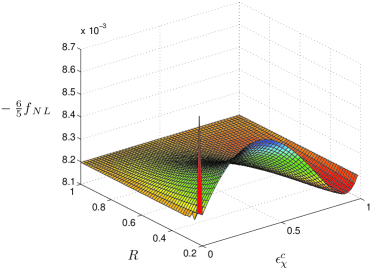
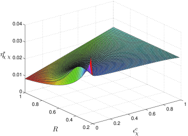
Figure 1: (color online). The non-linear parameter (69) and slow-roll parameter $\eta^{*}_{\chi\chi}$ (VI.4) as functions of $\epsilon^{c}_{\chi}$ and $R$, under the assumptions $N=60$ and $\epsilon^{c}_{\varphi}+\epsilon^{c}_{\chi}=1$. $R$ is defined as $R=\alpha/\beta$, the ratio of two parameters in the potential of this model.

In a practical simulation, we scan the region $0\leq\epsilon^{c}_{\chi}\leq 1$, $0.001\leq R\leq 1$ on a uniform grid with $101^{2}$ points. Some simulation results are illustrated in figure 1. When drawing the figure, we have imposed the slow-roll condition $\epsilon^{*}_{\varphi}<0.05$, $\epsilon^{*}_{\chi}<0.05$, $\eta^{*}_{\varphi\varphi}<0.05$, $\eta^{*}_{\chi\chi}<0.05$. In the limit $R=1$, they are in agreement with the analytical results $-6f_{\mathrm{NL}}^{(4)}/5=1/(2N+2)$, $\eta^{*}_{\chi\chi}=(2\epsilon^{c}_{\chi}+1)/(2N+2)$. One may also check the results in other limits analytically, such as $\epsilon^{c}_{\chi}\rightarrow 0$ or $\epsilon^{c}_{\chi}\rightarrow 1$. Theoretically, $R\rightarrow 0$ should correspond to an inflation model driven by one field $\varphi$. But our method does not apply to that limit, because it would violate the slow-roll condition for $\chi$.

From figure 1,we can see the non-linear parameter $f_{\mathrm{NL}}^{(4)}$ is suppressed by slow-roll parameters. Especially, in the neighborhood of $R=0$, the spikes of $f_{\mathrm{NL}}^{(4)}$ are located at the same positions as the spikes of $\eta^{*}_{\chi\chi}$. Such a coincidence continues to exist even if one relaxes the slow-roll condition. But there is no spike in similar graphs for $\epsilon^{*}_{\varphi}$, $\epsilon^{*}_{\chi}$ and $\eta^{*}_{\varphi\varphi}$. Actually, these spikes are mainly attributed to the enhancement of $f_{\mathrm{NL}}^{(4)}$ and $\eta^{*}_{\chi\chi}$ by $1/R$ in the small $R$ limit. After the parameter scanning and the numerical simulation, our lesson is that this model cannot generate a large non-Gaussianity unless the slow-roll condition breaks down.

VI.5 Non-separable Potential III: $W=\lambda e^{-\beta\varphi^{2}\chi^{2}}$, $e^{2b}=\alpha\varphi^{2}$

This is a special model of (26) with $p=0$, $\nu=-1$, $q=-1$. As in the previous subsection, we assume $N=60$ and $\epsilon^{c}_{\varphi}+\epsilon^{c}_{\chi}=1$. Then from section V we get the relations

$$\frac{\epsilon_{\varphi}}{\epsilon_{\chi}}=\alpha\chi^{2},\leavevmode\nobreak\ \leavevmode\nobreak\ \leavevmode\nobreak\ \leavevmode\nobreak\ \frac{\epsilon_{\chi}^{2}}{\epsilon_{\varphi}}=\frac{2M_{p}^{2}\beta^{2}}{\alpha^{2}}\varphi^{2},$$

$$\frac{4M_{p}^{2}\beta}{\alpha}=\frac{1}{N}\ln\left(\frac{\epsilon^{c}_{\varphi}\epsilon^{*}_{\chi}}{\epsilon^{c}_{\chi}\epsilon^{*}_{\varphi}}\right)=\epsilon_{\chi}\sqrt{\frac{\epsilon_{b}}{\epsilon_{\varphi}}},$$

$$\frac{1}{2}\sqrt{\frac{\epsilon_{b}}{\epsilon_{\varphi}}}=2-\frac{\eta_{\chi\chi}}{\epsilon_{\chi}}=2-\frac{\eta_{\varphi\varphi}}{\epsilon_{\varphi}}=1-\frac{\eta_{\varphi\chi}}{2\sqrt{\epsilon_{\varphi}\epsilon_{\chi}}},$$ (70)

$$u = 1-v=\frac{\epsilon^{c}_{\chi}\epsilon^{*}_{\varphi}}{\epsilon^{*}_{\chi}},$$

$$\mathcal{A} = -\frac{\epsilon^{*2}_{\varphi}\epsilon^{c}_{\varphi}\epsilon^{c2}_{\chi}}{2\epsilon^{*2}_{\chi}}\frac{4M_{p}^{2}\beta}{\alpha},$$ (71)

$$-\frac{6}{5}f_{\mathrm{NL}}^{(4)}=(\epsilon^{*}_{\chi}u^{2}+\epsilon^{*}_{\varphi}v^{2})^{-2}\biggl{[}\frac{\epsilon^{*}_{\varphi}}{2}\frac{4M_{p}^{2}\beta}{\alpha}(\epsilon^{*}_{\chi}u^{3}+\epsilon^{*}_{\varphi}v^{3}+2\epsilon^{*}_{\varphi}uv^{2})+2\mathcal{A}(\epsilon^{*}_{\chi}u-\epsilon^{*}_{\varphi}v)^{2}\biggr{]}.$$ (72)

For the present model, equation (10) gives

$$\ln\left(\frac{\varphi_{c}^{2}}{\varphi_{*}^{2}}\right)=\alpha(\chi_{c}^{2}-\chi_{*}^{2}),$$ (73)

that is

$$\ln\left(\frac{\epsilon^{c2}_{\chi}\epsilon^{*}_{\varphi}}{\epsilon^{c}_{\varphi}\epsilon^{*2}_{\chi}}\right)=\frac{\epsilon^{c}_{\varphi}}{\epsilon^{c}_{\chi}}-\frac{\epsilon^{*}_{\varphi}}{\epsilon^{*}_{\chi}}.$$ (74)

If we introduce the notations $R=(\epsilon^{c}_{\chi}\epsilon^{*}_{\varphi})/(\epsilon^{c}_{\varphi}\epsilon^{*}_{\chi})$, then combining it with equation (74) and the condition $\epsilon^{c}_{\varphi}+\epsilon^{c}_{\chi}=1$, we can express $\epsilon^{*}_{\varphi}$, $\epsilon^{*}_{\chi}$ and $f_{\mathrm{NL}}^{(4)}$ in terms of $\epsilon^{c}_{\varphi}$, $\epsilon^{c}_{\chi}$ and $R$,

$$\epsilon^{*}_{\varphi} = R^{2}\epsilon^{c}_{\varphi}\exp\left[\frac{(R-1)\epsilon^{c}_{\varphi}}{\epsilon^{c}_{\chi}}\right],$$

$$\epsilon^{*}_{\chi} = R\epsilon^{c}_{\chi}\exp\left[\frac{(R-1)\epsilon^{c}_{\varphi}}{\epsilon^{c}_{\chi}}\right],$$ (75)

$$-\frac{6}{5}f_{\mathrm{NL}}^{(4)}=\frac{1}{N}\ln\left(\frac{1}{R}\right)\frac{1-R\epsilon^{c}_{\varphi}+R^{2}(R-1)\epsilon^{c3}_{\varphi}-2R^{2}(R-1)^{2}\epsilon^{c5}_{\varphi}}{2[1-R\epsilon^{c}_{\varphi}+R(R-1)\epsilon^{c2}_{\varphi}]^{2}}.$$ (76)

On the basis of equation (VI.5), we deduce that $\ln(1/R)/N$ should be positive and suppressed by slow-roll parameters. In particular,

$$\eta^{*}_{\varphi\varphi} = 2\epsilon^{*}_{\varphi}-\frac{R\epsilon^{c}_{\varphi}}{\epsilon^{c}_{\chi}}\frac{1}{N}\ln\left(\frac{1}{R}\right),$$ (77)

$$\eta^{*}_{\chi\chi} = 2\epsilon^{*}_{\chi}-\frac{1}{N}\ln\left(\frac{1}{R}\right).$$ (78)

Thus we focus on the region $0<R<1$.

As indicated by the above analysis, if we are interested only in the non-linear parameter and slow-roll parameters, this model has two free parameters after using our assumptions and equations of motion. They will be chosen as $\epsilon^{c}_{\chi}$ and $R$ in our simulation, just like in the previous subsection. But we should warn that, compared with the previous subsection, the notation $R$ has a distinct meaning in the current subsection.

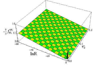
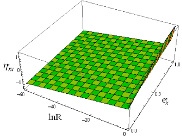
Figure 2: (color online). The non-linear parameter (76) and slow-roll parameter $\eta^{*}_{\chi\chi}$ (78) as functions of $\epsilon^{c}_{\chi}$ and $R$, under the assumptions $N=60$ and $\epsilon^{c}_{\varphi}+\epsilon^{c}_{\chi}=1$. $R$ is defined as $R=(\epsilon^{c}_{\chi}\epsilon^{*}_{\varphi})/(\epsilon^{c}_{\varphi}\epsilon^{*}_{\chi})$, and it is plotted in logarithmic scale.

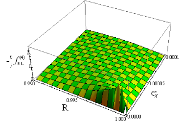
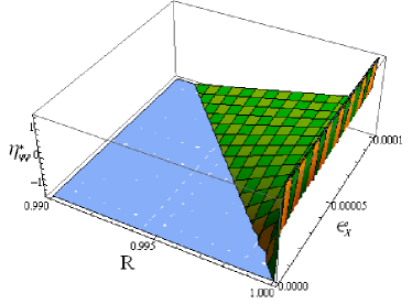
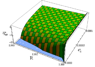
Figure 3: (color online). The non-linear parameter (76) and slow-roll parameter $\eta^{*}_{\varphi\varphi}$ (77) as functions of $\epsilon^{c}_{\chi}$ and $R$ near the corner $\epsilon^{c}_{\chi}\rightarrow 0$, $R\rightarrow 1$, under the assumptions $N=60$ and $\epsilon^{c}_{\varphi}+\epsilon^{c}_{\chi}=1$. $R$ is defined as $R=(\epsilon^{c}_{\chi}\epsilon^{*}_{\varphi})/(\epsilon^{c}_{\varphi}\epsilon^{*}_{\chi})$, and it is plotted in linear scale. In the middle and the lower graphs, the regions with $\eta^{*}_{\varphi\varphi}<-1.5$ and $\eta^{*}_{\varphi\varphi}<-10.5$ respectively are cut off.

The parameter scanning is illustrated by figures 2 and 3. In figure 2, parameter $R$ decreases exponentially from 1 to $e^{-60}$. In this process, the non-linear parameter grows roughly proportional to $\ln(1/R)$ while the slow-roll condition $|\eta^{*}_{\chi\chi}|\ll 1$ is violated gradually. This phenomenon agrees with equations (78) and (76), both of whose amplitude are enhanced by the factor $\ln(1/R)/N$ when $R$ is small. In figure 2,we find a sharp spike for the non-linear parameter in the corner $\epsilon^{c}_{\chi}\rightarrow 0$, $R\rightarrow 1$. Figure 3 is drawn to zoom in this corner, with $R$ scaled linearly. As shown by this figure, the spike dwells in a position violating the slow-roll condition $|\eta^{*}_{\varphi\varphi}|\ll 1$. Therefore, the non-linear parameter in this model must be small once the slow-roll condition $\epsilon^{*}_{i}\ll 1$, $\epsilon^{*}_{b}\ll 1$, $|\eta^{*}_{ij}|\ll 1$ ($i,j=\varphi,\chi$) is imposed.

VII Summary

In this paper, we investigated a class of two-field slow-roll inflation models whose non-linear parameter is analytically calculable.

In our convention of notations, we collected some well-known but necessary knowledge in section II. Slightly generalizing the method of Vernizzi:2006ve ; Choi:2007su , we showed in section III how their method could be utilized in a larger class of models satisfying two ansatzes, namely (15) and (20). In subsections III.1 and III.2 we proposed models meeting these ansatzes. We put our models in the form of $W(w)$ with $w=U(\varphi)+V(\chi)$ in subsection III.1 and with $w=U(\varphi)V(\chi)$ in subsection III.2. At first glance, these are two different classes of models. But in fact they are two dual forms of the same class of models, just as proved in subsection III.3. In a succinct form, our models can be summarized by equations (22) and (26), whose non-linear parameters were worked out in sections IV and V respectively, see equations (41) and (50). Under simplistic assumptions, we found no large non-Gaussianity in these models.

As a double check, we reduced the expression (41) for non-linear parameter to the additive potential in subsection VI.1, and (50) to multiplicative potential in subsection VI.2. The resulting non-linear parameters match with Vernizzi:2006ve ; Choi:2007su , confirming our calculations. In subsection VI.3, for a special class of models, we generalized Polarski and Starobinsky’s relation (58). For more specific models, we scanned the parameter space to evaluate the non-linear parameter, as shown by figures in subsections VI.4 and VI.5. In the scanning, we assumed the $e$-folding number $N=60$ and the inflation terminates at $-\dot{H}/H^{2}=1$. For the models we studied in subsections VI.4 and VI.5, the non-linear parameter $-6f_{\mathrm{NL}}^{(4)}/5$ always takes a small positive value under the slow-roll approximation.

References

• (1) A. H. Guth, Phys. Rev.  D 23, 347 (1981).
• (2) A. D. Linde, Phys. Lett.  B 108, 389 (1982).
• (3) A. Albrecht and P. J. Steinhardt, Phys. Rev. Lett.  48, 1220 (1982).
• (4) E. Komatsu et al., arXiv:1001.4538 [astro-ph.CO].
• (5) F. L. Bezrukov and M. Shaposhnikov, Phys. Lett.  B 659, 703 (2008) [arXiv:0710.3755 [hep-th]].
• (6) A. De Simone, M. P. Hertzberg and F. Wilczek, Phys. Lett.  B 678, 1 (2009) [arXiv:0812.4946 [hep-ph]].
• (7) S. Kachru, R. Kallosh, A. D. Linde, J. M. Maldacena, L. P. McAllister and S. P. Trivedi, JCAP 0310, 013 (2003) [arXiv:hep-th/0308055].
• (8) P. Chingangbam and Q. G. Huang, JCAP 0904, 031 (2009) [arXiv:0902.2619 [astro-ph.CO]].
• (9) Q. G. Huang, JCAP 0905, 005 (2009) [arXiv:0903.1542 [hep-th]].
• (10) X. Gao and B. Hu, JCAP 0908, 012 (2009) [arXiv:0903.1920 [astro-ph.CO]].
• (11) Y. F. Cai and H. Y. Xia, Phys. Lett.  B 677, 226 (2009) [arXiv:0904.0062 [hep-th]].
• (12) Q. G. Huang, JCAP 0906, 035 (2009) [arXiv:0904.2649 [hep-th]].
• (13) X. Gao and F. Xu, JCAP 0907, 042 (2009) [arXiv:0905.0405 [hep-th]].
• (14) X. Chen, B. Hu, M. x. Huang, G. Shiu and Y. Wang, JCAP 0908, 008 (2009) [arXiv:0905.3494 [astro-ph.CO]].
• (15) T. Matsuda, Class. Quant. Grav.  26, 145016 (2009) [arXiv:0906.0643 [hep-th]].
• (16) X. Gao, M. Li and C. Lin, JCAP 0911, 007 (2009) [arXiv:0906.1345 [astro-ph.CO]].
• (17) X. Gao, JCAP 1002, 019 (2010) [arXiv:0908.4035 [hep-th]].
• (18) K. Enqvist and T. Takahashi, JCAP 0912, 001 (2009) [arXiv:0909.5362 [astro-ph.CO]].
• (19) X. Chen and Y. Wang, JCAP 1004, 027 (2010) [arXiv:0911.3380 [hep-th]].
• (20) J. O. Gong, C. Lin and Y. Wang, JCAP 1003, 004 (2010) [arXiv:0912.2796 [astro-ph.CO]].
• (21) J. Garcia-Bellido and D. Wands, Phys. Rev.  D 53, 5437 (1996) [arXiv:astro-ph/9511029].
• (22) C. T. Byrnes and D. Wands, Phys. Rev.  D 74, 043529 (2006) [arXiv:astro-ph/0605679].
• (23) G. I. Rigopoulos, E. P. S. Shellard and B. J. W. van Tent, Phys. Rev.  D 76, 083512 (2007) [arXiv:astro-ph/0511041].
• (24) F. Vernizzi and D. Wands, JCAP 0605, 019 (2006) [arXiv:astro-ph/0603799].
• (25) C. T. Byrnes, K. Y. Choi and L. M. H. Hall, JCAP 0810, 008 (2008) [arXiv:0807.1101 [astro-ph]].
• (26) C. T. Byrnes, K. Y. Choi and L. M. H. Hall, JCAP 0902, 017 (2009) [arXiv:0812.0807 [astro-ph]].
• (27) C. T. Byrnes and G. Tasinato, JCAP 0908, 016 (2009) [arXiv:0906.0767 [astro-ph.CO]].
• (28) C. T. Byrnes and K. Y. Choi, Adv. Astron.  2010, 724525 (2010) [arXiv:1002.3110 [astro-ph.CO]].
• (29) F. Bernardeau and J. P. Uzan, Phys. Rev.  D 66, 103506 (2002) [arXiv:hep-ph/0207295].
• (30) F. Bernardeau and J. P. Uzan, Phys. Rev.  D 67, 121301 (2003) [arXiv:astro-ph/0209330].
• (31) H. R. S. Cogollo, Y. Rodriguez and C. A. Valenzuela-Toledo, JCAP 0808, 029 (2008) [arXiv:0806.1546 [astro-ph]].
• (32) Y. Rodriguez and C. A. Valenzuela-Toledo, Phys. Rev.  D 81, 023531 (2010) [arXiv:0811.4092 [astro-ph]].
• (33) D. H. Lyth and Y. Rodriguez, Phys. Rev. Lett.  95, 121302 (2005) [arXiv:astro-ph/0504045].
• (34) K. Y. Choi, L. M. H. Hall and C. van de Bruck, JCAP 0702, 029 (2007) [arXiv:astro-ph/0701247].
• (35) F. Di Marco and F. Finelli, Phys. Rev.  D 71, 123502 (2005) [arXiv:astro-ph/0505198].
• (36) J. C. Hwang and H. Noh, Phys. Rev.  D 71, 063536 (2005) [arXiv:gr-qc/0412126].
• (37) X. Ji and T. Wang, Phys. Rev.  D 79, 103525 (2009) [arXiv:0903.0379 [hep-th]].
• (38) http://www.rssd.esa.int/index.php?project=Planck
• (39) http://cmbpol.uchicago.edu/
• (40) D. Seery and J. E. Lidsey, JCAP 0509, 011 (2005) [arXiv:astro-ph/0506056].
• (41) D. Polarski and A. A. Starobinsky, Nucl. Phys.  B 385, 623 (1992).
• (42) D. Langlois, Phys. Rev.  D 59, 123512 (1999) [arXiv:astro-ph/9906080].