Soliton-like solutions to the ordinary Schroedinger equation${}^{\>({\dagger})}$

Michel Zamboni-Rached,

DMO, FEEC, UNICAMP, Campinas, SP, Brasil

and

Erasmo Recami

Facoltà di Ingegneria, Università statale di Bergamo, Bergamo, Italy;

and INFN—Sezione di Milano, Milan, Italy.

Abstract  –  In recent times it has been paid attention to the fact that (linear) wave equations admit of “soliton-like” solutions, known as Localized Waves or Non-diffracting Waves, which propagate without distortion in one direction. Such Localized Solutions (existing also for K-G or Dirac equations) are a priori suitable, more than gaussian’s, for describing elementary particle motion.  In this paper we show that, mutatis mutandis, Localized Solutions exist even for the ordinary Schroedinger equation within standard Quantum Mechanics; and we obtain both approximate and exact solutions, also setting forth for them particular examples.  In the ideal case such solutions bear infinite energy, as well as plane or spherical waves: we show therefore how to obtain finite-energy solutions.  At last, we briefly consider solutions for a particle moving in the presence of a potential.

PACS nos.:  03.65.-w ;  03.75.-b ;  03.65.Ta

Keywords: Schroedinger equation; Quantum mechanics; Localized waves; X-shaped waves; Bessel beams; X-waves; Localized beams; Localized pulses; Localized Wavepackets

1 Introduction

Recently it has been shown —as it had been already realized in old times[1]— that not only nonlinear, but also a large class of linear equations (including, in particular, the wave equations) admit of “soliton-like” solutions.  Those solutions[2] are localized, and travel along their propagation axis practically without diffracting (at least until a certain field-depth[2,3,4]): Such wavelets were indeed called “undistorted progressing waves” by Courant and Hilbert[1]. Let us recall that their peak-velocity $V$ can assume any values[5,6,2] $0\leq V\leq\infty$, even if we are mainly interested here in their localization properties rather than in their group-velocity.  In the case of wave equations, the localized solutions more easy to be constructed in exact form resulted to be the so-called “(superluminal) X-shaped” ones (see Refs.[4,7,8,2], and refs. therein).

The X-shaped waves, long ago predicted[6] to exist within Special Relativity (SR), have been first mathematically constructed[9,2] as solutions to the wave equations in Acoustics[4], and later on in Electromagnetism (namely, to the Maxwell equations[7]), and soon after produced experimentally[10].  Only very recently, subluminal localized solutions have been suitably worked out in exact form[11], even for the case of zero speed (“Frozen Waves”).[12]

It was soon thought that, since the mentioned solutions to the wave equations are non-diffractive and particle-like, they may well be related to elementary particles (and to their wave nature)[13,14]. And, in fact, localized solutions have been found for Klein-Gordon and for Dirac equations[13,14].

However, little work[15] has been done, as far as we know, for the (different) case of the Schroedinger equation. Indeed, the relation between the energy $E$ and the impulse magnitude $p\equiv|\mbox{\boldmath$p$}|$ is quadratic [$E=p^{2}/(2m)\/$] in the non-relativistic case, like in Schroedinger’s, at variance with the relativistic one. But, as we were saying, the nondiffracting solutions, which are essentially superpositions of Bessel beams and are currently called Localized Waves, would be quite apt at describing elementary particles: much more than the gaussian waves. In this paper we show that indeed, mutatis mutandis, Localized Solutions exist even for the ordinary Schroedinger equation within standard Quantum Mechanics; and we obtain both approximate and exact solutions, also setting forth for them particular examples. In the ideal case such solutions bear infinite energy, as well as spherical or plane waves: we shall therefore show how to obtain finite-energy solutions.  At last, we shall briefly consider solutions for a particle moving in the presence of a potential.

Before going on, let us recall that, in the time-independent realm —or, rather, when the dependence on time is only harmonic, i.e., for monochromatic solutions—, the (quantum, non-relativistic) Schroedinger equation is mathematically identical to the (classical, relativistic) Helmholtz equation[16].  And many trains of localized X-shaped pulses have been found, as superpositions of solutions to the Helmholtz equation, which propagate, for instance, along cylindrical or co-axial waveguides[17];  but we shall skip all the cases[18] of this type, even if interesting, since we are concerned here with propagation in free space, even when in the presence of an ordinary potential.  Let us also mention that, in the general time-dependent case, that is, in the case of pulses, the Schroedinger and the ordinary wave equation are no longer mathematically identical, since the time derivative results to be of the fist order in the former and of the second order in the latter. [It has been shown that, nevertheless, at least in some cases[19], they still share various classes of analogous solutions, differing only in their spreading properties[19]]. Moreover, the Schroedinger equation implies the existence of an intrinsic dispersion relation even for free particles.

Another difference, to be kept here in mind, between the wave and the Schroedinger equations is that the solutions to the wave equation suffer only diffraction (and no dispersion) in the vacuum, while those of the Schroedinger equation suffer also (an intrinsic) dispersion even in the vacuum.

Let us repeat that the majority of the ideal localized solutions we are going to construct are endowed with infinite energy. We shall treat also a finite-energy case only towards the end of this paper: In fact, infinite-energy solutions themselves, even without truncating them in space and time, results to be rather useful for describing wavepackets in regions not too extended in the transverse direction; as we shall see below.

2 Bessel beams as localized solutions (LS) to the Schroedinger equation

Let us consider the Schroedinger equation for a free particle (an electron, for example)

$$\mbox{\boldmath$\nabla$}^{2}\psi+{{2im}\over\hbar}\,{{\partial\psi}\over{\partial t}}\;=\;0\;.$$ (1)

If we confine ourselves to solutions of the type

$\psi(\rho,z,\varphi;t)\;=\;F(\rho,z,\varphi)\;{\rm e}^{-iEt/\hbar}\;,$

their spatial part $F$ obeys the reduced equation

$$\mbox{\boldmath$\nabla$}^{2}F+k^{2}F\;=\;0\;,$$ (2)

with  $k^{2}\equiv p^{2}/\hbar^{2}$  and  $p^{2}=2mE$ (quantity $p\equiv|\mbox{\boldmath$p$}|$ being the particle momentum, and therefore $k\equiv|\mbox{\boldmath$k$}|$ the total wavenumber).  Equation (2) is nothing but the Helmholtz equation, for which various simple localized-beam solutions (LS) are already known: In particular, the so-called Bessel beams[2], which have been experimentally produced since long[20].

Namely, let us now look —as usual— for solutions (cylindrically symmetric with respect to [w.r.t.] the $z$-axis) of the form

$\psi(\rho,z;t)\;=\;R(\rho)\ Z(z)\ T(t)\;,$

and explicitly indicate, mainly for clarity’s sake, the subsequent steps.  Equation (1) then becomes

$$\left[{1\over{\rho R}}{\partial\over{\partial\rho}}\left(\rho{{\partial R}\over{\partial\rho}}\right)+{1\over z}{{\partial^{2}Z}\over{\partial z^{2}}}\right]\;=\;-i{{2m}\over\hbar}{1\over T}{{\partial T}\over{\partial t}}$$ (3)

so that

$$-{{i2m}\over{\hbar T}}{{\partial T}\over{\partial t}}=-k^{2}\ \Longrightarrow\ T={\rm e}^{-iEt/\hbar}$$ (4)

where, let us repeat, $E=p^{2}/(2m)=k^{2}\hbar^{2}/(2m)$ (and in fact the last exponential is often written as $\exp{[-i\omega t]}$).

Analogously, we have

$${1\over{\rho R}}{\partial\over{\partial\rho}}\left(\rho{{\partial R}\over{\partial\rho}}\right)+k^{2}\;=\;-{1\over z}{{\partial^{2}z}\over{\partial z^{2}}}$$ (5)

and therefore

$$-{1\over z}{{\partial^{2}z}\over{\partial z^{2}}}\;=\;k_{z}^{2}\ \Longrightarrow\ \displaystyle{z={\rm e}^{izk_{z}}}\;,$$ (6)

where the constant $k_{z}\equiv k_{\parallel}=p_{\parallel}/\hbar\equiv p_{z}/\hbar$ is the longitudinal wavenumber.  We will suppose $k_{z}\geq 0$, that is, $p_{z}\geq 0$, to ensure that we deal with forward traveling beams only.

As a consequence, the (transverse) function $R=R(\rho)$ obeys the equation

$${1\over{\rho}}{\partial\over{\partial\rho}}\left(\rho{{\partial R}\over{\partial\rho}}\right)+(k^{2}-k_{z}^{2})R\;=\;0$$ (7)

which is a Bessel differential equation admitting as solution the Bessel function

$$R(\rho)\;=\;J_{0}(\rho k_{\rho})\;,$$ (8)

where the constant $k_{\rho}\equiv k_{\perp}\equiv p_{\perp}/\hbar$ is the transverse wavenumber, and

$$k_{\rho}^{2}=k^{2}-k_{z}^{2}\equiv 2mE/{\hbar^{2}}-k_{z}^{2}\;.$$ (9)

To avoid any divergencies, it must be $k_{\rho}^{2}\geq 0$, that is, $k^{2}\geq k_{z}^{2}$; namely, it must hold [see (a) in Fig.1] the constraint

$$E\,\geq\,{p_{z}^{2}\over{2m}}$$ (10)

[Notice that, to avoid the appearance of evanescent waves, one should postulate $k_{z}$ to be real; but such a condition is already included in our previous assumption that $k_{z}\geq 0$].  In the following, to simplify the notations, we shall also put [$p\equiv\hbar k\,$]:

$$p_{\rho}\,\equiv\,p_{\perp}\ .$$

The solution is therefore:

$$\psi(\rho,z;t)\;=\;J_{0}(\rho p_{\rho}/\hbar)\;\exp{[i(zp_{z}-Et)/\hbar]}$$ (11)

together with condition (9).  Equation (11) can be regarded as a Bessel beam solution to the Schroedinger equation.  This result is not surprising, since —once we suppose the whole time variation to be expressed by the function $\exp{[i\omega t]}$— both the ordinary wave equation and the Schroedinger equation transform into the Helmholtz equation.  Actually, the only difference between the Bessel beam solutions to the wave and to the Schroedinger equation consists in the different relationships among frequency, longitudinal, and transverse wavenumber; in other words (with $E\equiv\omega\hbar$):

$p_{\rho}^{2}\;=\;E^{2}/c^{2}-p_{z}^{2}\ \ \ \ \ {\rm for\ the\ wave\ equation};$ (12a)

$p_{\rho}^{2}\;=\;2mE-p_{z}^{2}\ \ \ \ \ \ {\rm for\ the\ Schroedinger\ equation}.\$   (12b)

In the case of beams, the experimental production of LSs to the Schroedinger equation can be similar to the one exploited for the LSs to the wave equations (e.g., in Optics, or Acoustics): Cf., e.g. Figure 1.2 in the first one of Refs.[8], and refs. therein, where the simple case of a source consisting in an array of circular slits, or rings, were considered.  In the Table we refer to a Bessel beam of photons, and a Bessel beam of (e.g.) electrons, respectively. We list therein the relevant quantities having a role, e.g., in Electromagnetism, and the corresponding ones for the Schroedinger equation’s spatial part $\hbar^{2}\mbox{\boldmath$\nabla$}^{2}F+2mE\,F=0$, with $F=R(\rho)\;Z(z)\,$. The second and the fourth lines have been written down for the simple Durnin et al.’s case, when the Bessel beam is produced by an annular slit (illuminated by a plane wave) located in the focus of a lens[20].

WAVE EQUATION	SCHROEDINGER EQUATION
$k\;=\;{\omega\over c}$	$p\;=\;\sqrt{2mE}$
$k_{\rho}\,\simeq\,{r\over f}\,k$	$p_{\rho}\simeq{r\over f}\,p$
$k_{\rho}^{2}\;=\;{\omega^{2}\over c^{2}}-k_{z}^{2}$	$p_{\rho}^{2}\;=\;2mE-p_{z}^{2}$
$k_{z}^{2}\;=\;{\omega^{2}\over c^{2}}(1-{r^{2}\over f^{2}})$	$p_{z}^{2}\;=\;2mE(1-{r^{2}\over f^{2}})$

In this Table, quantity $f$ is the focal distance of the lens (for instance, an ordinary lens in optics; and a magnetic lens in the case of Schroedinger charged wavepackets), and $r$ is the radius of the considered ring. [In connection with the last line of the Table, let us recall that in the wave equation case the phase-velocity $\omega/k_{z}$ is almost independent of the frequency (at least for limited frequency intervals, like in optics), and one gets a constant group-velocity and an easy way to build up X-shaped waves. By contrast, in the Schroedinger case, the phase-velocity of each (monochromatic) Bessel beam depends on the frequency, and this makes it difficult to generate an “X-wave” (i.e., a wave depending on $z$ and $t$ only via the quantity $z-Vt$) by using simple methods, as Durnin et al.’s, based on Bessel beams superposition. In the case of charged particles, one should compensate such a velocity variation by suitably modifying the focal distance $f$ of the Durnin’s lens, e.g. on having recourse to an additional magnetic, or electric, lens.]

Before going on, let us stress that one could easily eliminate the restriction of axial symmetry: In such a case, in fact, solution (11) would become

$\psi(\rho,z,\varphi;t)\;=\;J_{n}(\rho p_{\rho}/\hbar)\ \displaystyle{{\rm e}^{izp_{z}/\hbar}\,{\rm e}^{-iEt/\hbar}\,{\rm e}^{in\varphi}}\;,$

with $n$ an integer.  The investigation of not cylindrically-symmetric solutions is interesting especially in the case of localized pulses (cf. Sect.3): and we shall deal with them below.

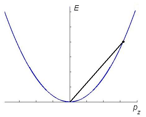
Figure 1: The parabola and the chosen straight-line have equations $E=p_{z}^{2}/(2m)$ and $E=Vp_{z}$, respectively. The intersection of our straight-line with the parabola corresponds to the value $E=2mV^{2}$.  The allowed region is the one internal to the parabola, since it must be $E\geq p_{z}^{2}/(2m)$.

3 Localized pulses as solutions to the Schroedinger equation (approximate method)

Localized (non-dispersive, besides non-diffracting) pulses can be constructed, as solutions to the Schroedinger equation, both by having recourse to the standard “paraxial approximation”, and in an exact, analytic way.  Let us start with the approximate method.

Let us go back, then, to our Bessel beam solution (11), with condition (10).  We can obtain localized (non-dispersive) pulses, as solutions to Schroedinger’s equation, by suitably superposing the beam solutions (11), and by selecting in the plane $(p_{z},E)$ the straight-line [see Fig.1]:

$$E\;=\;Vp_{z}\;;\ \ \ \ \ \ \ \ \ \ \ \ \ \ \ \ \ (p_{z}\geq 0)\ ,$$ (13)

vith $V$ a chosen constant speed; so that from eq.(10) one gets the important condition

$$E\;\leq\;2mV^{2}$$ (14)

and eq.(11) can consequently be written

$\psi(\rho,\zeta)\;=\;J_{0}(\rho p_{\rho}/\hbar)\;\exp{[ip_{z}\zeta/\hbar]}$ (11’)

where now  $p_{\rho}^{2}=(2mE-p_{z}^{2})=E(2m-E/V^{2})$  and we introduced the new variable

$$\zeta\;\equiv\;z-Vt\;.$$ (15)

Localized-wave solutions can be therefore obtained through the superposition (see Fig.1):

$$\Psi(\rho,\zeta)\;=\;{\cal N}\int_{0}^{2mV^{2}}{\rm d}E\;J_{0}\left(\rho\sqrt{{E\over\hbar^{2}}(2m-{E\over V^{2}})}\right)\;\exp{[{i{E\over{\hbar V}}\zeta}]}\;S(E)$$ (16)

the weight-function $S(E)$ being a suitable energy-spectrum (with the dimensions, as usual, of the inverse of an Energy), while ${\cal N}$ is a “normalization” constant which normalizes to 1 the peak-value of $|\Psi|^{2}$ and (since it multiplies a dimensionless integral) bears the dimensions $[{\cal N}]=[L^{3/2}]$, to respect the ordinary meaning of ${|\Psi(\rho,\zeta)|}^{2}$.  It should be noted that we are integrating, in the space ($p_{z},E$) along the straight-line (13), that is, $E=Vp_{z}\$.  This corresponds to superposing Bessel beams all endowed with the same phase-velocity $V_{\rm ph}\equiv V$.  The resulting pulse will possess $V$ as its group-velocity (namely, as its peak-velocity), since it is well-known that, when the phase-velocity $V_{\rm ph}$ does not depend on the energy or frequency, the resulting pulse happens to travel with the group-velocity $V_{\rm g}\equiv\partial\omega/\partial k_{z}=V_{\rm ph}\equiv V$: cf. refs.[17,2,21] and refs. therein.  Due to constraint (14), we are actually integrating along our straight-line from $0$ to $2mV^{2}$ (see Fig.1).

It is important also to note explicitly that each solution $\Psi(\rho,\zeta)$ given by eq.(16), depending on $z$ (and $t$) only via the variable $\zeta\equiv z-Vt$, does represent a pulse that appear with a constant shape to an observer traveling with speed $V$ along the wave motion-line $z$:  in other words, it represents a pulse which propagates rigidly along $z$.  Therefore, eqs.(16) are already —as desired– non-dispersing and non-diffracting (”localized”) solutions to the Schroedinger equation.

Integrals (16), however, appear difficult to be analytically performed, independently of the spectrum $S(E)$ chosen.

To overcome this difficulty, let us rewrite eq.(11’) as a function of $p_{\rho}$ only, by exploiting eq.(12b), which can be written  $E^{2}/V^{2}-2mE+p_{\rho}^{2}=0$,  and yields

$$E\;=\;mV^{2}\left(1+\sqrt{1-{p_{\rho}^{2}\over p_{\rho{\rm max}}^{2}}}\right)\;,$$ (17)

where

$$p_{\rho{\rm max}}\;=\;mV\;,$$

as it comes by deriving eq.(12b) with respect to $E$.

Therefore, eq.(11’) becomes

$\psi(\rho,\zeta)\;=\;J_{0}(\rho p_{\rho}/\hbar)\,\exp{[i{{mV}\over\hbar}\,\zeta\,\sqrt{1-{p_{\rho}^{2}\over{m^{2}V^{2}}}}\;]}\ S(p_{\rho}/\hbar)\ \displaystyle{{\rm e}^{i{{mV}\over\hbar}\zeta}}$ (11”)

with $0\leq p_{\rho}\leq p_{\rho{\rm max}}$, where, let us repeat, $p_{\rho{\rm max}}=mV$.  Then, the Localized Solutions will be written as

$$\Psi(\rho,\zeta)\;=\;{\cal N}{\rm e}^{imV\zeta/\hbar}\int_{0}^{mV}{\rm d}p_{\rho}\;J_{0}({{\rho p_{\rho}}\over\hbar})\;S(p_{\rho})\;\exp{\left[{{imV}\over\hbar}\,\zeta\,\sqrt{1-{p_{\rho}^{2}\over{m^{2}V^{2}}}}\right]}\;.$$ (18)

Let us notice that, in the new variable $p_{\rho}$, the Bessel function, previously written as in eq.(16), gets, as we have seen, the simplified expression $J_{0}(\rho p_{\rho})$.

It is now enough to choose a weight-function $S$ that is strongly bumped around the value $p_{\rho}$, in the interval [$0,mV$], with

$$p_{\rho}\ll mV\;,$$ (19)

for being able to integrate from $0$ to $\infty$ with a negligible error.  Namely, let us now adopt the so-called paraxial approximation.  Under condition (19), one can approximate the exponential factor as follows:

$mV\displaystyle{\sqrt{1-{p_{\rho}^{2}\over{m^{2}V^{2}}}}\,\simeq\,mV-{1\over 2}{p_{\rho}^{2}\over{mV}}}\;,$

so that eq.(18) can be eventually written in terms of an integration from $0$ to $\infty$:

$$\Psi(\rho,\zeta)\;=\;{\cal N}{\rm e}^{2imV\zeta/\hbar}\int_{0}^{\infty}{\rm d}p_{\rho}\;J_{0}({{\rho p_{\rho}}\over\hbar})\ S(p_{\rho})\ \exp{[i{{p_{\rho}^{2}}\over{2\hbar mV}}\zeta]}\;.$$ (20)

Let us now examine various special cases of weight-functions $S(p_{\rho})$ obeying the previous conditions: that is, well localized around a value $p_{\rho}\ll mV$.

3.1 Some examples of approximate Localized Solutions to the Schroedinger equation (paraxial approximation)

As already claimed, we are for the moment adopting the paraxial approximation, since it yields good, and interesting enough, results: Only in the subsequent Sections we shall go on to the exact, analytical approach.

First of all, let us consider the simple spectrum

$$S(p_{\rho})\;=\;4q\,p_{\rho}\,\displaystyle{{\rm e}^{-qp_{\rho}^{2}}}$$ (21)

(with the dimensions, now, of the inverse of an Impulse), with

$q\equiv\displaystyle{{\alpha\over{m^{2}V^{2}}}}$ (22a)

so that the above conditions merely imply the dimensionless constant $a$ to be

$\alpha\gg 1\;.\$ (22b)

In this case, also the total spectral-width $\Delta p_{\rho}$ results to be $\Delta p_{\rho}\ll mV$: and this too supports the fact that our integral can indeed run till $\infty$.  In eq.(20), one can then perform (analytically) the integration, and get the solutions

$$\Psi(\rho,\zeta)\,\simeq\,{\cal N}\ 4q\hbar^{2}\;{\rm e}^{2imV\zeta/\hbar}\;{1\over{2Q}}\;\exp{[-{\rho^{2}\over{4\hbar(q\hbar-i{1\over{mV}}\zeta)}}]}\;,$$ (23)

quantity $q$ being still the one defined in eq.(22a), with $\alpha\gg 1$; while function $Q$ is

$$Q\,\equiv\,\hbar(q\hbar-{i\over{2mV}}\,\zeta)\;.$$ (24)

Equation (23) constitutes an interesting solution of the Schroedinger equation: It describes a wavepacket rigidly moving with the chosen speed $V$.  The maximum of its intensity $|\Psi|^{2}$ occurs at

$$\rho\;=\;0;\ \ \ \ \ \zeta\;=\;0\;,$$

and therefore also such a maximum travels with the speed $V$, as expected (since $\zeta=z-Vt$).  For $\zeta=0$ one gets [$\alpha\gg 1$]:

$$|\Psi(\rho,\zeta=0)|^{2}\,\simeq\,{{\cal N}}^{2}\;4\;\exp{[-{{\rho^{2}}\over{2q\hbar^{2}}}]}\;,$$ (25)

and the transverse localization $\Delta\rho$ of the wavepacket results to be

$\Delta\rho\;=\;\displaystyle{{\hbar\over{mV}}}\,\sqrt{2\alpha}\;,$ (25’)

which shows also the rôle of $\alpha$ (and therefore of $q$) in regulating the wavepacket (constant) transverse total width.

By contrast, putting $\rho=0$ into eq.(23), we end up with the expression [still with $\alpha\gg 1$]:

$$|\Psi(\rho=0,\zeta)|^{2}\,\simeq\,{{\cal N}}^{2}\;4\;\displaystyle{{{q^{2}\hbar^{2}}\over{q^{2}\hbar^{2}+{1\over{4m^{2}V^{2}}}\zeta^{2}}}}\;,$$ (26)

which corresponds to

$$\Delta\zeta\;=\;\sqrt{e^{2}-1}\;{{2\alpha\hbar}\over{mV}}\ .$$

Solution (26) is represented in Fig.2.

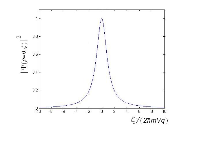
Figure 2: Behavior of $|\Psi(\rho=0,\zeta)|^{2}$ in eq.(26), as a function of $\zeta/(2\hbar qmV)$.

Let us briefly consider a few further possible spectra.  We shall go on confining ourselves to the simple case of cylindrical symmetry, but analogous solutions can be easily found also for more general non-symmetrical cases.

As the second option, let us choose the new spectrum

$$S(p_{\rho})\;=\;\displaystyle{{1\over p_{\rho}}\,\displaystyle{{\rm e}^{-qp_{\rho}^{2}}}}\;,$$ (27)

quantity $q$ being defined in eq.(22a), and condition (22b) being enforced, so that $q\gg 1/(m^{2}V^{2})$ and, again, $\Delta p_{\rho}\ll mV$.  Equation (20) yields the new solution

$$\Psi(\rho,\zeta)\,\simeq\,{\cal N}\ {1\over 2}\;\gamma\left(0,{\rho^{2}\over{4Q}}\right)\ \exp{[{{i2mV}\over\hbar}\,\zeta]}\;,$$ (28)

where function $Q$ is defined in eq.(24), and $\gamma$, here, is the “incomplete gamma function”.[22]

$$\gamma(0,{\cal A})\;=\;-\gamma(-1,{\cal A})-{\cal A}^{-1}\,{\rm e}^{-{\cal A}}$$

with

$\begin{array}[]{clr}\gamma(-1,{\cal A})&\equiv-{\cal A}^{-1}\,{\rm e}^{-{\cal A}}\;\Phi(1,0;{\cal A})\\ &\equiv-{\cal A}^{-1}\,{\rm e}^{-{\cal A}}[1-\Phi(1,0;{\cal A})]\;,\end{array}$

function $\Phi$ being the “Probability Integral”, that in the present case can be defined as

$\Phi(1,0;{\cal A})\,\equiv\,\displaystyle{{1\over\Gamma(1)}\;\int_{0}^{\infty}{\rm d}x\ {{\alpha-{\rm e}^{-{\cal A}x}}\over{1-{\rm e}^{-x}}}}\;.$

The maximum, also for solution (27), occurs at $\rho=\zeta=0$.

As a third option, we choose

$$S(p_{\rho})\;=\;\displaystyle{{qp_{\rho}}\,{\rm e}^{-qp_{\rho}^{2}}\,I_{0}({{sp_{\rho}}\over\hbar})}\,$$ (29)

always with $\alpha\gg 1$, quantity $q$ being given by eq.(22a), $s$ a constant with the dimensions of a Length (regulating the spectrum bandwidth), and $I_{0}$ being the Modified Bessel Function;   one gets from eq.(20) the further new solution

$$\Psi(\rho,\zeta)\,\simeq\,{\cal N}\ {{q\hbar}\over{2Q}}\,{\rm e}^{{{i2mV}\over\hbar}\,\zeta}\,\exp{\left[{{s^{2}-\rho^{2}}\over{4Q}}\right]}\;J_{0}\left({{s\rho}\over{2Q}}\right)\;.$$ (30)

As the last option, let us choose

$$S(p_{\rho})\;=\;\displaystyle{qp_{\rho}\,{\rm e}^{-qp_{\rho}^{2}}\,J_{0}(sp_{\rho})}\;,$$ (31)

from eq.(20) it follows the fourth solution

$$\Psi(\rho,\zeta)\simeq{\cal N}\ {q\over{2Q}}\,{\rm e}^{{{i2mV}\over\hbar}\,\zeta}\,\exp{\left[-{{s^{2}+\rho^{2}}\over{4Q}}\right]}\ I_{0}\left({{s\rho}\over{2Q}}\right)\;.$$ (32)

4 Exact Localized Solutions to the Schroedinger equation (for arbitrary frequency spectra)

Our aim is now to construct new analytical solutions to the Schroedinger equation, by following an exact (not approximate) approach.  Let us, then, go back to eq.(1), and to its Bessel-beam solution (11), where, as before, relation (12b) holds:  $p_{\rho}=\sqrt{2mE-p_{z}^{2}}$, with $E=\omega\hbar$.

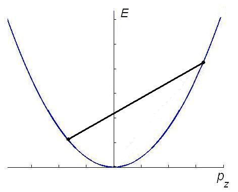
Figure 3: This time, the parabola and the chosen straight-line have equations $E=p_{z}^{2}/(2m)$ and $E=Vp_{z}+b$, respectively. The intersections of this straight-line with the parabola are now two, whose corresponding values are given in eq.(33b).  Inside the parabola $p_{\rho}^{2}\geq 0$.

The condition for obtaining a Localized Solution (cf. Fig.3) is that

$E\;=\;Vp_{z}+b\;,$ (33a)

with $b$ a positive constant (bearing the dimensions of an Energy, and regulating the position of the chosen straight-line in the plane $(E,p_{z})$); which corresponds in particular, on using eq.(12b), to the adoption of the integration limits

$E_{\pm}\;=\;mV^{2}\left(1\pm\sqrt{1+{{2b}\over{mV^{2}}}}\right)+b\;.$ (33b)

Localized Solutions can therefore be obtained by the following superpositions (integrations over the frequency, or the energy) of Bessel-beam solutions:

$$\Psi(\rho,z,\zeta)\;=\;\displaystyle{{\rm e}^{{{-ib}\over\hbar V}z}}\;\int_{E_{-}}^{E_{+}}{\rm d}E\;J_{0}(\rho p_{\rho}/\hbar)\;S(E)\;\displaystyle{{\rm e}^{i{E\over\hbar V}\zeta}}\;,$$ (34)

together with

$$p_{\rho}\;=\;{1\over V}\,\sqrt{-E^{2}+(2mV^{2}+2b)E-b^{2}}\;.$$ (35)

Notice that the in eq.(34) [as well as in eq.(39) below], the solution $\Psi$ depends on $z$, besides via $\zeta$, only via a phase factor; the modulus $|\Psi|$ of $\Psi$ goes on depending on $z$ (and on $t$) only through the variable $\zeta\equiv z-Vt$.

4.1 Particular exact Localized Solutions

We want now to re-write the integral ${\cal{I}}$ appearing in the r.h.s. of eq.(34) so that its integration limits are $-1$ and $+1$, respectively; that is, in the form

${\cal{I}}\;=\;\displaystyle{\int_{-1}^{1}{\rm d}u\;S(u)\;J_{0}({{\rho\sqrt{P}}\over\hbar}\sqrt{1-u^{2}})\>{\rm e}^{i\,f(\zeta)\,u}}\;,$

quantity $f(\zeta)$ being an arbitrary dimensionless function. To obtain this, we have to look for a transformation of variables [with $A$ and $B$ constants, with the dimensions of an Energy, to be determined]

$$E\;=\;Au+B$$ (36)

such that

$p_{\rho}^{2}\;=\;P(1-u^{2})\;;\ \ \ \ \ u_{+}=1\;;\ \ \ \ \ u_{-}=-1\;,$ (36’)

$P$ being a suitable constant (with the dimensions of an Impulse square).  On writing  $V^{2}p_{\rho}^{2}\;=\;E\,(\hbar V^{2}M-E)-b^{2}$,  with $\hbar M\equiv 2m+2b/{V^{2}}$,  after some algebra one finds that it must be

$$A\;=\;\sqrt{P}\;V\;;\ \ \ \ \ B\;=\;mV^{2}+b\;;\ \ \ \ \ P\;=\;m^{2}V^{2}+2mb\;.$$ (37)

Indeed, one can verify (by some more algebra) that eqs.(36)-(37) imply, as desired, that  $u_{-}\;=\;-1$  and  $u_{+}\;=\;1$.

In conclusion, the transformation

$$E\;=\;mV^{2}\sqrt{1+{{2b}\over{mV^{2}}}}\ \;u+mV^{2}+b$$ (38)

does actually allow writing solution (34) in the form [recall that $E=Au+B\Longrightarrow{\rm d}E=A{\rm d}u$]

$$\Psi(\rho,\eta,\zeta)\;=\;{\cal N}\ A\;\displaystyle{{\rm e}^{{{imV}\over\hbar}\eta}}\;\int_{-1}^{1}{\rm d}u\;S(u)\;J_{0}({\rho\over\hbar}\sqrt{P}\sqrt{1-u^{2}})\;\displaystyle{{\rm e}^{{{iA\zeta}\over{\hbar V}}u}}\;,$$ (39)

with

$$\eta\equiv z-vt\;,$$

where $v\equiv V+b/(mV)$.  Equation (39) is exactly, analytically integrable when $S$ is a constant or a suitable exponential.

Let us choose the complex exponential function (which will easily enter as an element in a Fourier expansion)

$${\overline{S}(E)}\;=\;a_{n}\;\displaystyle{{\rm e}^{{{2\pi i}\over D}nE}}\;,$$ (40)

with $n$ an integer, and $D\equiv E_{+}-E_{-}=2mV^{2}\;\sqrt{1+2b/(mV^{2})}$, while $a_{n}$ are constant quantities (with dimensions of the inverse of an Energy).  On remembering that $E=Au+B$, such a spectrum can be written in terms of $u$ as

${\overline{S}}(u)\;=\;a_{n}\;\displaystyle{{\rm e}^{i\pi nu}\;{\rm e}^{i{{2\pi}\over D}nB}}$ (40’)

(still with the dimensions of an inverse Energy).  After some more algebra, the analytic exact solution to the Schroedinger equation, corresponding to spectrum (41), results to be[11]

$$\Psi(\rho,\eta,\zeta)\;=\;{\cal N}a_{n}\;{2A}\;{\sin{Z}\over Z}\;\displaystyle{{\rm e}^{{{imV}\over\hbar}\eta}\;{\rm e}^{i{{2\pi}\over D}nB}}\;\;,$$ (41)

where $A,\ B,\ P$ are given by eqs.(37) and

$$Z\,\equiv\,\sqrt{\left({A\over{\hbar V}}\zeta+n\pi\right)^{2}+{P\over\hbar^{2}}\rho^{2}}\;.$$ (42)

Equation (41), as we have just seen, is a particular exact Localized Solution to the Schroedinger equation; but we are going to utilize it essentially as an element of suitable superpositions.  Before going on, however, we wish to depict in Figs.4 an elementary solution: namely, the square magnitude of the simple solution corresponding, in eq.(34), to the real exponential

$$S(E)\;=\;s_{0}\;\displaystyle{\exp[a(E-E_{+})]}\;,$$ (43)

$a$ being a positive number, endowed with the dimensions of an inverse Energy, as well as $s_{0}$.  When $a=0$, one ends up with a solutions similar to Mckinnon’s[23].  Spectrum (43) is exponentially concentrated in the proximity of $E_{+}$, where it reaches its maximum value; and becomes more and more concentrated (on the left of $E_{+}$, of course) as the arbitrarily chosen value of $a$ increases.  To perform the integration in eq.(34), it is once more useful to operate the variable transformation (36) and go on to eq.(39), spectrum (43) assuming now the form

$$S(u)\;=\;s_{0}\;e^{-aE_{+}}\;e^{aB}\;e^{aAu}\;.$$

Performing the integration in eq.(39), by a process similar to the one which led us to eq.(41), in the present case we get

$\Psi(\rho,\eta,\zeta)\;=\;{\cal N}s_{0}2V\sqrt{P}\;\displaystyle{\exp[i{{mV}\over{\hbar}}\eta]\ \exp[-aV\sqrt{P}]\ {{\sin Y}\over Y}}$ (44a)

where

$Y\;\equiv\;{{\sqrt{P}}\over\hbar}\,\sqrt{\rho^{2}-(\hbar aV+i\zeta)^{2}}\;,$ (44b)

quantity $P$ having been defined in eq.(37); and one should remember that $\eta\equiv z-vt$ is a function of $b$.

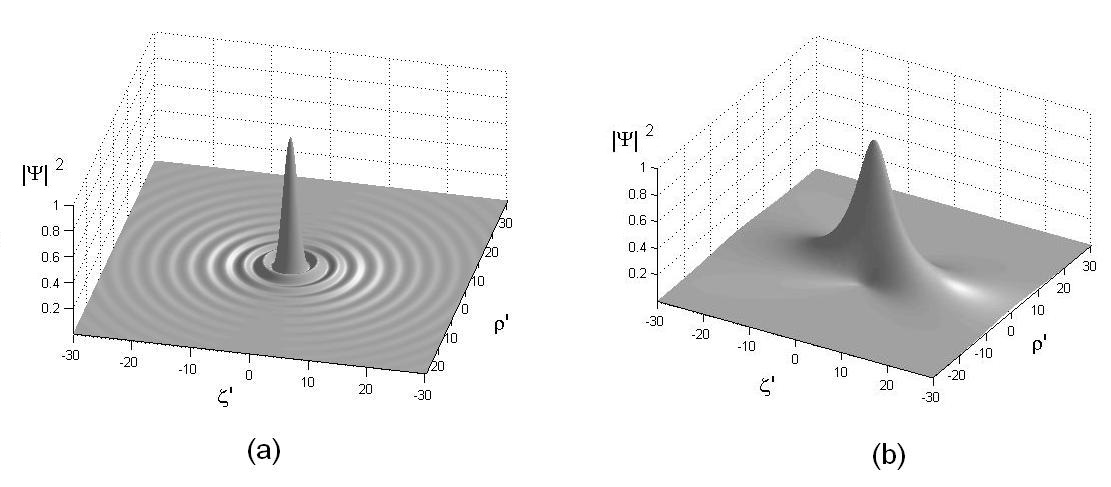
Figure 4: In these figures we depict an elementary solution: namely, the square magnitude of the simplified solution, eq.(44a), corresponding to the real spectrum $S(u)=s_{0}\exp[(E-E_{+})a]$, as a function of $\rho^{\prime}\equiv\rho\sqrt{P}/\hbar$ and of $\zeta^{\prime}\equiv\zeta\sqrt{P}/\hbar$. Quantity $a$ is a positive number [when $a=0$ one ends up with a solutions similar to Mckinnon’s[23]], while $b$ for simplicity has be chosen equal to zero.  Figure (a) corresponds to $a=E_{+}/5$, while figure (b) corresponds to $a=5E_{+}$.  For the properties of the spectral function (43), see the text.

Equations (44) appear to be the simplest closed-form solutions (see Figs.4) to the Schroedinger equation, since they do not need any recourse to series expansions of the type exploited in the following Subsection. However, the solutions that we shell construct below can correspond to spectra more general than (43); for instance, to the gaussian spectrum, which possesses two advantage w.r.t. spectrum (43): it can be easily centered around any value of $u$, that is, around any value $\bar{E}$ of $E$ in the interval [$E_{-},E_{+}$], and, when increasing its concentration in the surrounding of $\bar{E}$, its “spot” transverse width does not increase, at variance with what happens for spectrum (43). Anyway, the exact solutions (44) are noticeable, since they are really the simplest ones.

Some physical (interesting) comments on the results in eqs.(44) and Figs.4 will appear elsewhere. Here, let us add only a few further Figures and some brief comments. Let us first recall that, as predicted in the first one of Refs.[6], the Localized (Nondiffracting) Solutions to the ordinary wave equations resulted to be roughly ball-like when their peak-velocity is subluminal[11], and X-shaped[4,7] when superluminal.

Now, normalizing $\rho$ and $\zeta$, we can write eq.(44b) as

$$Y\;=\;\sqrt{{\rho^{\prime}}^{2}-({\overline{A}}+i\zeta^{\prime})^{2}}$$

with  $\rho^{\prime}\equiv\sqrt{P}\rho/\hbar$  and  $\zeta^{\prime}\equiv\sqrt{P}\zeta/\hbar$,  quantity $P$ being given by the last one of eqs.(37), namely $P=m^{2}V^{2}+2mb$,  while  ${\overline{A}}\equiv aA=\sqrt{P}aV$.  For simplicity, let us confine ourselves to the case $b=0$, forgetting now about the more interesting cases with $b\neq 0$;  therefore, it will hold the simple relation

$${\overline{A}}=maV^{2}\ .$$

In the present case of the Schroedinger equation, we can observe the following.

If we choose ${\overline{A}}=0$, which can be associated with $V=0$, we get the solutions in Figs.5: that is, a ball-like structure.

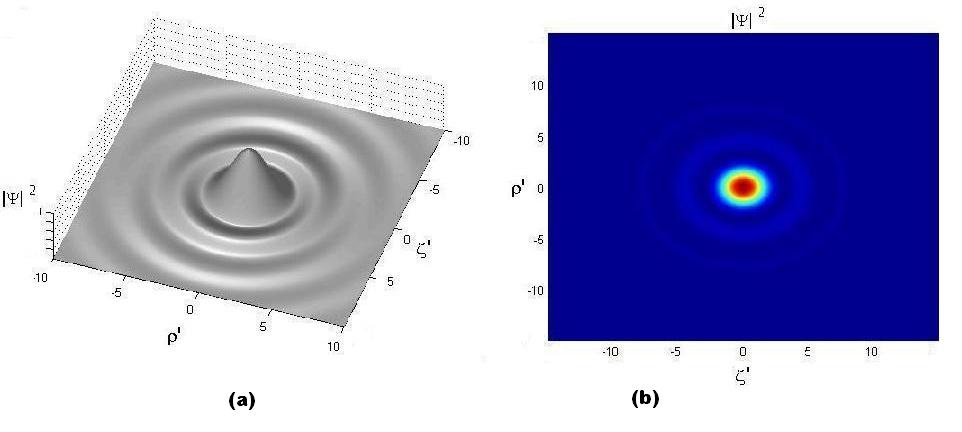
Figure 5: In these, and the following Figures 6, 7 and 8, we depict the square magnitude of some more solutions of the type (44a), normalized with respect to $\rho$ and $\zeta$; still assuming for simplicity $b=0$, so that ${\overline{A}}=maV^{2}$. The present figures show the “ball-like” structure that one gets, as expected, when ${\overline{A}}=0$ (see the text, also for the definitions of $\rho^{\prime}$ and $\zeta^{\prime}$).  Fig.(b) shows the projection on the plane ($\rho^{\prime},\ \zeta^{\prime}$) of the 3D plot shown in Fig.(a).

By contrast, if we increase the value of ${\overline{A}}$, by choosing e.g. ${\overline{A}}=20$ (which can be associated with larger speeds), one notices that also a X-shaped structure starts to contribute: See, e.g., Fig.6.

Figure 6: The solution, under all the previous conditions, with an increased value of ${\overline{A}}$, namely with ${\overline{A}}=20$. An X-shaped structure starts to appear, contributing to the general form of the solution (see the text).

To have a preliminary idea of the “internal structure” of our soliton-like solutions to the (ordinary) Schroedinger equation, let us plot, instead of the square magnitude of $\Psi$, its real or imaginary part: Let us choose its real part, or rather the square of its real part.  Then even in the ${\overline{A}}=0$ case one starts to see the appearance of the X shape, which becomes more and more evident as the value of ${\overline{A}}$ increases: In Figs.7 we show the projections on the plane ($\zeta^{\prime},\ \rho^{\prime}$) of the real-part square for the solutions with ${\overline{A}}=5$ and ${\overline{A}}=50$, respectively.  Further attention to such aspects will be paid elsewhere.

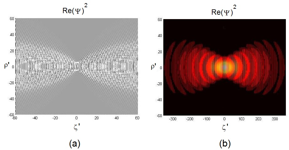
Figure 7: To get a preliminary idea of the “internal structure” of our soliton-like solutions, it is useful to have recourse (see the text) to the real part of $\Psi$. In these Figures we plot the projections on the plane ($\zeta^{\prime},\ \rho^{\prime}$) of the real-part square for the solutions with ${\overline{A}}=5$ (figure (a)) and ${\overline{A}}=50$ (figure (b)), respectively.

But the (square of the) real part of $\Psi$ does show, in 3D, also some “internal oscillations”: Cf., e.g., Fig.8 corresponding to the value ${\overline{A}}=5$.  We shall face elsewhere, however, topics like their possible connections with the de Broglie picture of quantum particles, et alia.

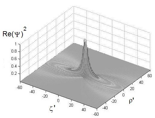
Figure 8: The (square of the) real part of $\Psi$ shows, in 3D, also some “internal oscillations”: this Figure corresponds, e.g., to the value ${\overline{A}}=5$.

4.2 A general exact Localized Solution

Let us go back to our spectrum $S(E)$ in eq.(40). Since in our fundamental equation (34) the integration interval is limited [$E_{-}<E<E_{+}$], in such an interval any spectral function $S(E)$ whatever can be expanded into the Fourier series

$$S(E)\;=\;\sum_{n=-\infty}^{\infty}\,a_{n}\,\displaystyle{{\rm e}^{i{{2\pi}\over D}nE}}\;,$$ (45)

with

$$a_{n}\;=\;{1\over D}\displaystyle{\int_{E_{-}}^{E_{+}}{\rm d}E\;S(E)\;{\rm e}^{-i{{2\pi}\over D}nE}}\;,$$ (46)

quantity $S(E)$ being an arbitrary function, and $D$ being still defined as $D\equiv E_{+}-E_{-}$.

Inserting eq.(45) into eq.(34), and following the same procedure exploited in the previous Subsection (in particular, going on again from $E$ to the new variable $u$), we end up —after normalization— with the general exact localized solution to the Schroedinger equation:

$$\Psi(\rho,\eta,\zeta)\;=\;{\cal N}\,{2A}\,\displaystyle{e^{i{{mV}\over{\hbar}}\eta}}\ \sum_{n=-\infty}^{\infty}\,a_{n}\;\displaystyle{\exp{[{i{{2\pi}\over D}nB}]}}\;{\sin{Z}\over Z}\;,$$ (47)

where $Z$ is defined in eq.(42), and the coefficients $a_{n}$ are given by eq.(46).

It is worthwhile to note that, even when truncating the series in eq.(47) at a certain value $n=N$, the solutions obtained is still an exact LS of the Schroedinger equation!

5 About finite-energy Localized Solutions to the Schroedinger equation

The solutions found above, even if very instructive, are ideal solutions which are not square integrable; and cannot be accepted in QM. It is important, therefore, to show how to construct finite-energy solutions.

Let us obtain localized solution to the Schroedinger equation endowed with finite energy, by starting from eqs.(44). First of all, one has to integrate over $b$ by adopting a spectrum $S(b)$ strongly bumped around a value $b_{0}$: We already know, indeed, that spectra of this type are required in order to get solutions that are non-diffracting all along a certain field-depth.

Then, it can be easily seen that the finite-energy solution, $\Psi_{\rm fe}$, can be preliminarily written as

$$\Psi_{\rm fe}\;=\;{\cal N}\ {{s_{0}V\sqrt{P}}\over{iY}}\ (I_{-}-I_{+})\;,$$ (48)

where $I_{-}$ and $I_{+}$ are two (dimensionless) integrations over $b$ from 0 to infinity (quantity $b$ having been defined in eq.(33a), and therefore having the dimensions of an Energy), while $s_{0}$ appears in eq.(43).

Let us now pass from $b$, defined in eq.(33a), to the new variable $w\equiv\sqrt{P}$. One has to choose a spectrum $S(w)$ corresponding to a $S(b)$ concentrated around a specific value of $b$; let us therefore adopt the gaussian function

$${\cal S}(w)\;=\;{{m\sqrt{q}}\over{\sqrt{\pi}\hbar w}}\;\exp[-q(w-w_{0})^{2}]\;,$$ (49)

with $w_{0}>mV>0$.

When we go on from $b$ to the new variable $w\equiv\sqrt{P}$ (where $P$ depends on $b$), the two quantities $I_{-}$ and $I_{+}$ become integrations over $w$ from $mV$ to $\infty$. After further calculations, and using relation 3.322.1 in ref.[22], one obtains that

$$I_{\pm}\;=\;{{\sqrt{q}}\over{U}}\,e^{-qw_{0}}\,e^{{{imV}\over 2\hbar}z}\,\exp{[{W_{\pm}^{2}\over U^{2}}]}\ \left[1-\Phi\left({W_{\pm}\over U}+{{mV}\over{2}}U\right)\right]\;,$$ (50)

where

$$U\equiv 2\sqrt{q+{{i\hbar}\over{2m}}t}\,;\ \ \ \ \ W_{\pm}\equiv-2qw_{0}+aV\pm i{Y\over\sqrt{P}}\;,$$

quantity $Y$ having been defined in eq.(44b).

We have therefore shown that realistic (finite-energy) Localized Solutions exist also to the Schroedinger equation; they will be non-diffracting only till a certain finite distance (depth of field). The analysis of explicit, particular examples will be presented elsewhere.

6 The case of non-free particles

Let us consider now the case of a particle in the presence of a potential: for simplicity, let us confine ourselves to the case of a cylindrical potential.

Namely, let us consider the Schroedinger equation with a potential of the type $U(\rho)$:

$$-\frac{\hbar^{2}}{2m}\left(\nabla^{2}_{\bot}+\frac{\partial^{2}}{\partial z^{2}}\right)\psi+U(\rho)\psi-i\hbar\frac{\partial\psi}{\partial t}\;=\;0$$ (51)

Now, we can use the method of separation of variables writing $\psi=R(x,y)Z(z)T(t)$. With this, we get the well known solutions

$$T=\displaystyle{e^{-\frac{i}{\hbar}E\,t}}$$ (52)

$$Z=\displaystyle{e^{ip_{z}z/\hbar}}$$ (53)

and the eigenvalue equation

$$-\hbar^{2}\,\nabla^{2}_{\bot}R+2m\,U(\rho)\,R\;=\;\Lambda^{2}R$$ (54)

with

$$\Lambda^{2}\;=\;2mE-p_{z}^{2}$$ (55)

Supposing a potential $U(\rho)$ that only allows transverse bound states (as the parabolic potential), we will find eigenfunctions $R_{n}(x,y)$ and discrete (degenerate) eigenvalues $\Lambda_{n}^{2}$.

We can construct more general solutions

$$\Psi=\sum_{n}f_{n}R_{n}(x,y)e^{ik_{z}z/\hbar}e^{-\frac{i}{\hbar}Et}$$ (56)

with

$$2mE\;=\;p_{z}^{2}+\Lambda^{2}_{n}$$ (57)

Considering $p_{z}\geq 0$ (forward propagation), the constraint (57) defines a set of parabolas (something like the modes in a waveguide: Cf. Refs.16). Chosen a certain $\Lambda_{n}^{2}$, once a value for $p_{z}$ is given, the value of $E$ gets fixed.

To obtain from (56) a train of localized pulses, i.e., a wavefunction $\Psi(x,y,z-Vt)$, we must have

$$E\;=\;Vp_{z}$$ (58)

So, from conditions (57) and (58), $p_{z}$ must assume the values

$$p_{z}\;=\;mV\left(1\pm\sqrt{1-\frac{1}{m^{2}V^{2}}\Lambda_{n}^{2}}\right)$$ (59)

with

$$\Lambda_{n}\leq mV$$ (60)

Figure 9 illustrates the situation. The values to $E$ and $p_{z}$ that furnish localized pulse trains are given by the intersection between the parabolas defined by eq.(57) and the straight line defined by eqs.(58). Note that in these cases the series (56) will be always truncated (finite number of terms), due the condition (60). We also have to note that, for any given $\lambda_{n}^{2}$, one gets two possible values of $k_{z}$ (see eq.(59)), as it can be observed from Fig.9, in which the straight line cuts each parabola twice.

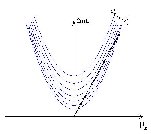
Figure 9: In the case of a particle in the presence of a cylindrical potential, the values to $E$ and $p_{z}$ that furnish Localized Pulse trains are given by the intersection between the parabolas in eq.(57) and the straight line in eq.(58): see the text. It can be noticed that, for any given $\lambda_{n}^{2}$, one gets two possible values of $k_{z}$ (cf. eq.(59)), since the straight line cuts each parabola twice.  See the text, and cf. also Refs.[17].

For our purpose, the superposition has to be

$$\Psi(x,y,z-Vt)\;=\;\sum_{n}f_{n}R_{n}(x,y)e^{ip_{zn}(z-Vt)/\hbar}$$ (61)

with

$$p_{z}\;=\;mV\left(1\pm\sqrt{1-\frac{1}{m^{2}V^{2}}\Lambda_{n}^{2}}\right)$$ (62)

and

$$\Lambda_{n}\leq mV$$ (63)

In principle, any set of coefficients $f_{n}$ will furnish trains of localized waves.

Observation1: If we look for a square-integrable wave function, we can start from superposition (56) and integrate its terms over $p_{z}$ around each $p_{zn}$, respectively (as we already did in our papers on X-type pulses propagating along wave-guides[17]). But in the present case, in general, the group-velocities defined at the points $p_{zn}$ will not be the same, as it happened in the waveguide case; and we will therefore meet a kind of intermodal dispersion, besides the group-velocity dispersion. Let us recall, incidentally, that such an intermodal dispersion did not occur in the case of X-type waves, traveling in metallic wave-guides, due the peculiar fact that the group-velocities defined at those points were always the same ). After the integration, we can obtain an envelope with a train of pulses (or just one pulse) inside it. The envelope will suffer dispersion, but the train of pulses inside it will not.

More general localized wave trains can be obtained using the relation $E\;=\;Vp_{z}+b$, with $b$ a positive constant.

In the case of potentials like $U(\rho)$, one can search for solutions with cylindrical symmetry, for simplicity. However, solutions without this symmetry can be investigated: and they will be interesting for an analysis of angular momentum.

7 Acknowledgments

The authors are grateful to Claudio Conti, Hugo E. Hernández-Figueroa e Peeter Saari for many stimulating contacts and discussions. After the completion of this work (see, e.g., our e-print arXiv:1008.3087[quant-ph]), we came to know that some work on the same topic, by following different paths, has been done also by I.B.Besieris and A.M.Shaarawi (“Localized traveling wave solutions to the 3D Schroedinger equation”: unpublished): And we are grateful to I.M.Besieris for such a piece of information.

References

- [1] H.Bateman: Electrical and Optical Wave Motion (Cambridge Univ.Press; Cambridge, 1915); R.Courant and D.Hilbert: Methods of Mathematical Physics (J.Wiley; New York, 1966), vol.2, p.760; J.A.Stratton: Electromagnetic Theory (McGraw-Hill; New York, 1941), p.356.
- [2] See, e.g., M.Z.Rached, E.Recami and H.E.Figueroa: “New localized Superluminal solutions to the wave equations with finite total energies and arbitrary frequencies” [arXiv e-print physics/0109062], European Physical Journal D21 (2002) 217-228, and refs. therein; H.E.H.Figueroa, M.Z.Rached and E.Recami (editors): Localized Waves (J.Wiley; New York, 2008), book of 386 pages; E.Recami and M.Z.Rached: “Localized Waves: A Review”, Advances in Imaging & Electron Physics (AIEP) 156 (2009) 235-355 [121 printed pages].
- [3] See, e.g., M.Z.Rached, “Analytical expressions for the longitudinal evolution of nondiffracting pulses truncated by finite apertures,” J. Opt. Soc. Am. A 23 (2006) 2166-2176, and refs. therein.
- [4] J.-y. Lu and J.F.Greenleaf: “Nondiffracting X-waves: Exact solutions to free-space scalar wave equation, and their finite aperture realizations”, IEEE Transactions in Ultrasonics Ferroelectricity and Frequency Control 39 (1992) 19-31.
- [5] Cf., e.g., R.Donnelly and R.W.Ziolkowski: “Designing localized waves”, Proceedings of the Royal Society of London A440 (1993) 541-565, and refs. therein.
- [6] A.O.Barut, G.D.Maccarrone and E.Recami, Nuovo Cimento A71 (1982) 509; E.Recami, Rivista N. Cim. 9(6), 1178 (1986), issue no.6, p.158 and pp.116-117; E.Recami, M.Zamboni-Rached and C.A.Dartora: Phys. Rev. E69 (2004) 027602, and refs. therein. Cf. also D.Mugnai, A.Ranfagni, R.Ruggeri, A.Agresti and E.Recami, Phys. Lett. A209 (1995) 227; E.Recami: “Superluminal waves and objects: An up-dated overview of the relevant experiments” [e-print arXiv:0804.1502], in press.
- [7] E.Recami: “On localized ‘X-shaped’ Superluminal solutions to Maxwell equations”, Physica A252 (1998) 586-610, and refs. therein. Cr. also J.-y.Lu, J.F.Greenleaf and E.Recami, “Limited diffraction solutions to Maxwell (and Schroedinger) equations”, arXiv e-print physics/9610012.
- [8] E.Recami, M.Z.Rached and H.E.H.Figueroa: “Localized waves: A historical and scientific introduction” [e-print arXiv:0708.1655], in Localized Waves, ed. by H.E.H.Figueroa, M.Z.Rached and E.Recami (J.Wiley; New York, 2008), Chapter 1, pp.1-41; M.Z.Rached, E.Recami & H.E.H.Figueroa: “Structure of the nondiffracting waves and some interesting applications” [e-print arXiv:0708.1209], in Localized Waves, ed. by H.E.H.Figueroa, M.Z.Rached and E.Recami (J.Wiley; New York, 2008), Chapter 2, pp.43-77.
- [9] See, e.g., W.Ziolkowski, I.M.Besieris and A.M.Shaarawi: “Aperture realizations of exact solutions to homogeneous wave-equations”, J. Opt. Soc. Am. A10 (1993) 75, Sects.5 and 6.
- [10] J.-y. Lu and J.F.Greenleaf: “Experimental verification of nondiffracting X-waves”, IEEE Transactions in Ultrasonics Ferroelectricity and Frequency Control 39 (1992) 441-446; P.Saari and K.Reivelt: “Evidence of X-shaped propagation-invariant localized light waves,” Physical Review Letters 79 (1997) 4135-4138. See also P.Bowlan, H.Valtna-Lukner, M.Lohmus, P.Piksarv, P.Saari and R.Trebino: “Pulses by frequency-resolved optical gating”, Opt. Lett. 34 (2009) 2276-2278.
- [11] M.Z.Rached and E.Recami: “Sub-luminal Wave Bullets: Exact Localized subluminal Solutions to the Wave Equations” [e-print arXiv:0709.2372], Physical Review A77 (2008) 033824. Cf. also C.J.R.Sheppard: “Generalized Bessel pulse beams”. J. Opt. Soc. Am. A19 (2002) 2218-2222.
- [12] M.Z.Rached, E.Recami and H.E.H.Figueroa: “Theory of ‘Frozen Waves’” [arXiv e-print physics/0502105], Journal of the Optical Society of America A22 (2005) 2465-2475; M.Z.Rached: “Stationary optical wave fields with arbitrary longitudinal shape, by superposing equal-frequency Bessel beams: Frozen Waves”, Optics Express 12 (2004) 4001-4006.
- [13] A.M.Shaarawi, I.M.Besieris and R.W.Ziolkowski: J. Math. Phys. 31 (1990) 2511-2519, especially Sect.VI; Nucl Phys. (Proc.Suppl.) B6 (1989) 255-258; Phys. Lett. A188 (1994) 218-224.
- [14] A.O.Barut: Phys. Lett. A143 (1990) 349; ibidem A171 (1992) 1-2; V.K.Ignatovich: Foundations of Physics 8 (1978) 565-571; A.O.Barut and A.Grant: “Quantum particle-like configurations of the electromagnetic field”, Found. Phys. Lett. 3 (1990) 303-310; A.O.Barut and A.J.Bracken: “Particle-like configurations of the electromagnetic field: an extension of de Broglie’s ideas”, Found. Phys. 22 (1992) 1267-1285. Cf. also A.O.Barut: in L. de Broglie, Heisenberg’s Uncertainties and the Probabilistic Interpretation of Wave Mechanics (Kluwer; Dordrecht, 1990); A.O.Barut: “Quantum theory of single events: Localized de Broglie–wavelets, Schroedinger waves and classical trajectories”, preprint IC/90/99 (ICTP; Trieste, 1990); P.Hillion: Phys. Lett. A172 (1992) 1.
- [15] Cf., e.g., C.Conti and S.Trillo: Phys. Rev. Lett. 92 (2004) 120404; C.Conti: “Generalition and nonlinear dynamics of X-waves of the Schroedinger equantion”, Phys. Rev. E70 (2004) 046613.
- [16] See, e.g., Th.Martin and R.Landauer: Phys. Rev. A 45 (1992) 2611; R.Y.Chiao, P.G. Kwiat and A.M.Steinberg: Physica B 175 (1991) 257; A.Ranfagni, D.Mugnai, P.Fabeni and G.P.Pazzi, Appl. Phys. Lett. 58 (1991) 774, and refs. therein. See also A.M. Steinberg, Phys. Rev. A52 (1995) 32.
- [17] M.Z.Rached, K.Z.Nóbrega, E.Recami and H.E.H.Figueroa: “Superluminal X-shaped beams propagating without distortion along a co-axial guide” [arXiv e-print physics/0209104], Physical Review E66 (2002) 046617 [10 pages]; M.Zamboni-Rached, E.Recami and F.Fontana: “Localized Superluminal solutions to Maxwell equations propagating along a normal-sized waveguide”, Phys. Rev. E64 (2001) 066603 [6 pages]; “Superluminal localized solutions to Maxwell equations propagating along a waveguide: The finite-energy case”, Phys. Rev. E67 (2003) 036620 [7 pages].
- [18] Cf. also A.P.L.Barbero, H.E.H.Figueroa and E.Recami: “On the propagation speed of evanescent modes”, Phys. Rev. E62 (2000) 8628-8635; G.Nimtz and A.Enders: J. de Physique-I 2 (1992) 1693 ; 3 (1993) 1089; G.Nimtz, A.Enders and H.Spieker: J. de Physique-I 4 (1994) 565; V.S.Olkhovsky, E.Recami and G.Salesi: “Tunneling through two successive barriers and the Hartman (Superluminal) effect” [arXiv e-print quant-ph/0002022], Europhysics Letters 57 (2002) 879-884; Y.Aharonov, N.Erez and B.Reznik: Phys. Rev. A65 (2002) 052124; S.Longhi, P.Laporta, M.Belmonte and E.Recami: “Measurement of Superluminal optical tunneling times in double-barrier photonic bandgaps” [arXiv e-print physics/0201013], Phys. Rev. E65 (2002) 046610 [6 pages]; E.Recami: “Superluminal tunneling through successive barriers. Does QM predict infinite group-velocities?”, Journal of Modern Optics 51 (2004) 913-923; V.S.Olkhovsky, E.Recami and A.K.Zaichenko: “Resonant and non-resonant tunneling through a double barrier” [arXiv e-print quant-th/0410128], Europhysics Letters 70 (2005) 712-718; M.Z.Rached and H.E.H.Figueroa, “A Rigorous analysis of Localized Wave propagation in optical fibers”, Opt. Commun. 191 (2001) 49-54.
- [19] V.S.Olkhovsky, E.Recami and J.Jakiel: “Unified time analysis of photon and nonrelativistic particle tunnelling”, Physics Reports 398 (2004) 133-178, and refs. therein.
- [20] J.Durnin, J.J.Miceli and J.H.Eberly: “Diffraction-free beams”, Physical Review Letters 58 (1987) 1499-1501; C.J.R.Sheppard and T.Wilson, “Gaussian-beam theory of lenses with annular aperture”, IEEE Journal on Microwaves, Optics and Acoustics 2 (1978) 105-112. See also C.J.R.Sheppard, ibidem 2 (1978) 163-166.
- [21] Ettore Majorana - Notes on Theoretical Physics, ed. by S.Esposito, E.Majorana jr., A. van der Merwe and E.Recami (Kluwer; Dordrecht and N.Y., 2003); book of 512 pages.
- [22] I.S.Gradshteyn and I.M.Ryzhik: Integrals, Series and Products, 4th edition (Ac.Press; New York, 1965).
- [23] L. Mackinnon: “A nondispersive de Broglie wave packet”, Found. Phys. 8 (1978) 157.