Unified description of perturbation theory and band center anomaly in one-dimensional Anderson localization

Abstract

We calculated numerically the localization length of one-dimensional Anderson model with diagonal disorder. For weak disorder, we showed that the localization length changes continuously as the energy changes from the band center to the boundary of the anomalous region near the band edge. We found that all the localization lengths for different disorder strengths and different energies collapse onto a single curve, which can be fitted by a simple equation. Thus the description of the perturbation theory and the band center anomaly were unified into this equation.

1 Introduction

Electronic transport properties, the motion of electrons, in a random potential are closely related to the phenomenon of localization. Since the pioneering work of Anderson [2] for disordered systems fifty years ago, Anderson localization has been applied to various fields including photonics and cold atoms [15]. However, even for the simplest one-dimensional case, we have not found exact analytical treatment for arbitrary disorder strengths and energies [14, 19, 9]. Accurate numerical approaches have been developed by using the quantum transfer matrix renormalization group method for finite temperature systems [25], the density matrix renormalization group method for interacting systems [20], and the integral equation method for systems in the thermodynamic limit [11], respectively. In this work we will give a unified description of the in-band (without the band edge anomalous region) behavior for the one-dimensional model with weak diagonal disorder. We study the problem with the help of a numerical method we developed earlier in Ref. [11], which was an application of the transfer matrix method [18] in localized phase in the thermodynamic limit.

The localization theory shows rigorously that all the eigenstates are exponentially localized for one-dimensional uncorrelated disordered systems. The single parameter scaling (SPS) theory [1] gave great insight into the properties of disordered systems. It argues that the dimensionless conductance $g$ is the only relevant parameter that controls its variation with system size $L$. SPS requires that the complete distribution function $p(g)$ should be determined by one single parameter. Originally, SPS was derived within the random phase approximation [3]. The finite size Lyapunov exponent $\tilde{\gamma}(L)=(1/2L)\ln(1+1/g)$ was proposed to be an appropriate scaling parameter (it approaches the nonrandom limit when $L\rightarrow\infty$ [17]). It is well-known that the random phase approximation fails at the band edges $E=\pm 2$ as well as the band center $E=0$ [21, 23]. Another length scale was suggested to give an appropriate criterion for the failure of SPS [8] and a relatively good scaling parameter was found for the non-SPS region [6].

For weak disorder, although $p(g)$ has two independent parameters which is in contrast with the case of strong disorder, it was found that one of them is a universal number [16]. Thus it is still SPS. There exists a perturbation theory in which the Lyapunov exponent depends on energy $E$ and disorder strength $W$ [24]

$$\gamma_{p}(E,W^{2})=\frac{W^{2}}{96(1-E^{2}/4)}.$$ (1)

At the band center, a revised perturbation gives [12, 5, 10]

$$\gamma(W^{2})=\frac{W^{2}}{105.045\cdots}.$$ (2)

There was no analytical expression which connects smoothly the above two perturbative results. To clarify the smooth crossover in between we study the Lyapunov exponent with two variables, the energy $E$ and the disorder strength $\sigma^{2}$ in this paper ($\sigma^{2}=W^{2}/12$). Furthermore, we only study the problem in the thermodynamic limit and thus the third variable, the size of a finite system, is not in consideration.

It was shown that for one-dimensional Anderson model with diagonal disorder, the band center is actually a band boundary adjoining two neighbor bands rather than the center of a single band, which is the reason for the fail of SPS near the band center. Therefore it is similar to the band edge [7]. This should also be why in Ref. [10] the authors used a four-step map at the band center. In our recent work, we proposed a parametrization method of the transfer matrix for one-dimensional Anderson model with diagonal disorder. Making use of this method, we obtained numerical results of the dependence of the Lyapunov exponent on energy and disorder strength in the thermodynamic limit within the localization regime. A remarkable coincidence of our numerical results with the existed results demonstrated the reliability and efficiency of our method [11]. For the anomalous region near the band center, there have been analytical results for $E\rightarrow 0$ and $E\gg\sigma^{2}$ through the scaled energy $E/\sigma^{2}$ [5]. In the present work, we will show the detailed numerical results about the anomalous behavior of the Lyapunov exponent with weak disorder near the band center by using our method, which coincides with the known analytical results; and we will give a simple equation to describe the behavior for arbitrary weak disorder strength and for all $E$ in the band except the anomalous region near the band edge through the parameter $E/\sigma^{2}$. Thus the band center anomaly and the perturbation theory are connected smoothly.

2 Parametrization method

Consider the one-dimensional Anderson model with diagonal disorder,

$$\psi_{i-1}+\psi_{i+1}=(E-\epsilon_{i})\psi_{i},$$ (3)

where $\psi_{i}$ is the electron wavefunction at site-$i$ and $\epsilon_{i}$ is the on-site energy from a random distribution $p_{\epsilon}(\epsilon)$. For the box distribution, $p_{\epsilon}(\epsilon)=1/W$, $|\epsilon|<W/2$, $\langle\epsilon^{2}\rangle=W^{2}/12$, and for the Gaussian distribution, $p_{\epsilon}(\epsilon)=(1/\sqrt{2\pi}\sigma)\exp(-\epsilon^{2}/2\sigma^{2})$, $\langle\epsilon^{2}\rangle=\sigma^{2}$. In the transfer matrix method, Eq. (3) can be written as

$$\Psi_{i+1}=\left(\begin{array}[]{c}\psi_{i+1}\\ \psi_{i}\end{array}\right)=\left(\begin{array}[]{cc}v_{i}&-1\\ 1&0\end{array}\right)\left(\begin{array}[]{c}\psi_{i}\\ \psi_{i-1}\end{array}\right)=\mathbf{T}_{i}\Psi_{i},$$ (4)

where $v_{i}=E-\epsilon_{i}$ and $\mathbf{T}_{i}$ is the transfer matrix.

Using a parametrization method of the transfer matrix proposed in our previous work [11], we can calculate the Lyapunov exponent in the thermodynamic limit within the localization regime. Let $\mathbf{M}_{L}=\mathbf{T}_{L}\mathbf{T}_{L-1}\cdots\mathbf{T}_{1}$. Then we can parameterize $\mathbf{M}\mathbf{M}^{t}$ as follows

$$\mathbf{U}(\theta_{L})\mathbf{M}_{L}\mathbf{M}^{t}_{L}\mathbf{U}(-\theta_{L})=\left(\begin{array}[]{cc}e^{\lambda_{L}}&\\ &e^{-\lambda_{L}}\end{array}\right),$$ (5)

where $\mathbf{M}^{t}$ is the transpose of $\mathbf{M}$ and

$$\mathbf{U}(\theta_{L})=\left(\begin{array}[]{cc}\cos\theta_{L}&-\sin\theta_{L}\\ \sin\theta_{L}&\cos\theta_{L}\end{array}\right).$$ (6)

The recursion relation of $\theta$ in large $L$ limit is

$$\tan\theta_{L+1}=\frac{1}{v_{L+1}-\tan\theta_{L}}.$$ (7)

The two parameters $\lambda$ and $\theta$ are what we need in order to calculate the Lyapunov exponent $\gamma$. The equations we obtained for the distribution function $p(\theta)$ and the Lyapunov exponent are

$$p(\theta)=\frac{1}{\sin^{2}\theta}\int p(\theta^{\prime})p_{v}(\frac{1}{\tan\theta}+\tan\theta^{\prime})\mathrm{d}\theta^{\prime}$$ (8)

$$\gamma=-\int p(\theta)\ln|\tan\theta|\mathrm{d}\theta$$ (9)

where $p_{v}(v)$ is the random distribution function of $v$. In this study we use the Gaussian distribution $p_{v}(v)=(1/\sqrt{2\pi}\sigma)\exp[-(v-E)^{2}/2\sigma^{2}]$ to solve Eq. (8) and to calculate $\gamma$ numerically for different $\sigma^{2}$ and different energy $E$.

3 Numerical results

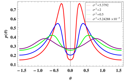
Figure 1: (Color online) Distribution $p(\theta)$ from Eq. (8) at fixed $E=0$ for the Gaussian distribution with decreasing $\sigma^{2}$.

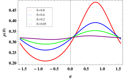
Figure 2: (Color online) Distribution $p(\theta)$ from Eq. (8) at fixed $\sigma^{2}=0.00125$ for the Gaussian distribution with decreasing $E$.

Fig. 1 and Fig. 2 illustrate the distribution functions $p(\theta)$ which were calculated as $p_{v}(v)$ being the Gaussian distribution. In Fig. 1, four curves of $E=0$ are plotted for different values of $\sigma^{2}$ decreased from 5.3792 to $5.24288\times 10^{-5}$; and in Fig. 2, four curves of $\sigma^{2}=0.00125$ are plotted for different values of $E$ decreased from 0.8 to 0.05. In Fig. 1, $p(\theta)$ becomes a stationary distribution when disorder is weak enough (the line of $\sigma^{2}=5.24288\times 10^{-5}$)

$$p(\theta)=\frac{1}{K(1/2)\sqrt{3+\cos 4\theta}},$$ (10)

where $K$ is the complete elliptic integral of the first kind [10]. There is a correspondence between $p(\theta)$ and the distribution of the reflection phase $\phi$ in Ref. [4], which gave similar plots, through the relation $\tan\theta=\cos(\phi/2)/\cos(\mu+\phi/2)$, where $2\cos\mu=E$. In Fig. 2, the expression of distribution $p(\theta)$ for the three larger values of $E$ is

$$p(\theta)=\frac{\sin\mu}{\pi(1-\cos\mu\sin 2\theta)},$$ (11)

corresponding to the uniform distribution for the perturbation theory [12, 10]. A recent numerical calculation [13] of the angle distribution function in Ref. [10] also gave a similar behavior. In our numerical approach we have set a relative precision $10^{-10}$ of $p(\theta)$.

For weak disorder we have known that the perturbation theory breaks down near the band center. It is clear in Fig. 3 that the distribution $p(\theta)$ of $E=0.05$ with $\sigma^{2}=0.00125$ deviates from Eq. (11), which means that the band center anomalous region extends up to $E>80\sigma^{2}$. In Figs. 1 and 2 we have demonstrated known results for the two limits $E/\sigma^{2}\rightarrow 0$ and $E/\sigma^{2}\rightarrow\infty$; and in Fig. 3 contribution of higher order terms to the curves in weak disorder perturbation becomes apparent for finite $E/\sigma^{2}$. In Ref. [22] the authors gave a complete accurate analysis of not only the localization length, but all higher moments of the distribution of the Lyapunov exponent for finite systems. It is natural to expect that the deviation from Eq. (11) comes from higher order terms in the perturbation given in Ref. [22]. And the present work will give an accurate equation for the localization length in the whole band except the band edge anomalous region.

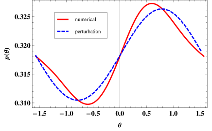
Figure 3: (Color online) Comparison of $p(\theta)$ between the numerical result and Eq. (11) ($E=0.05$ and $\sigma^{2}=0.00125$), which means that the standard perturbation theory fails when $E$ approaches $\sigma$.

To demonstrate the anomalous behavior near the band center, we plot $\gamma(E)$ with disorder strength $\sigma^{2}=0.005$ for $p_{v}(v)$ being the Gaussian distribution in Fig. 4. It shows clearly that in the vicinity of the band center the behavior of the Lyapunov exponent deviates from the perturbation result ($\gamma_{p}$ solid line) and when $E$ approaches zero it becomes the result of Eq. (2) smoothly [22]. Our numerical results coincides with the analytical results for the region near $E/\sigma^{2}\ll 1$ and $E/\sigma^{2}\gg 1$ [5]. We will present a quantitative description by collapsing the curves for different energies and disorder strengths through the parameter $E/\sigma^{2}$.

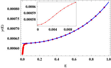
Figure 4: (Color online) $\gamma(E)$ with disorder strength $\sigma^{2}=0.005$ for $E<1$ and $p_{v}(v)$ as the Gaussian distribution. The solid line is the standard perturbation result. A magnified curve for $E<0.01$ is plotted in the inset.

Considering Eqs. (1) and (2) as well as the result shown in Fig. 4, we choose $y=1-\gamma/\gamma_{p}$ as a scaling parameter. $y$ is the relative difference between the perturbation result and the numerical result. To show all the values of $E/\sigma^{2}$ we use $x=\arctan(E/a\sigma^{2})$, where $a$ is a fitting coefficient. $x=0$ at the band center $E=0$ and $x=\pi/2$ for a finite energy when $E/\sigma^{2}\sim 1/\sigma^{2}\rightarrow\infty$ with $\sigma^{2}\rightarrow 0$. In Fig. 5 there are three groups of data and the fitting coefficient $a\approx 1.436$. Each group has a fixed weak disorder strength. All the data points merge into a single curve. Thus the in-band behavior can be described by a single scaling parameter for all weak disorder values of $\sigma^{2}$ as long as $E$ is not located in the band edge anomalous region. If the energy is in the band edge anomalous region, we found that $y$ deviates from the universal curve in Fig. 5, which was not shown here.

When $E$ approaches the boundary of the band center anomalous region, $\gamma$ becomes equal to the perturbation result $\gamma_{p}$, therefore $y\rightarrow 0$; when $E=0$, $y=1-96/105.045\approx 0.086$. So We expect that

$$y\approx(1-\frac{96}{105.045})\cos^{2}x,$$ (12)

where $\cos^{2}x=[1+(E/a\sigma^{2})^{2}]^{-1}$. Therefore the Lyapunov exponent for weak disorder and with energy in the band except near the band edge is

$$\gamma=f(\frac{E}{\sigma^{2}})\gamma_{p},$$ (13)

where $f(E/\sigma^{2})=1-0.086[1+(E/a\sigma^{2})^{2}]^{-1}+\cdots$. The difference in $\gamma$ is only $8.6\%$ for the $E=0$ and a finite energy. A quantitative description can be given: if we set the criterion for the breaking down of the perturbative result in Eq. (1) as $1\%$ difference in $\gamma$, then by Eq. (13) we obtain $|E|\gtrsim 4\sigma^{2}$ as the region for Eq. (1) to be considered as valid. It is $|E|\gtrsim 8D$ which is in agreement with the $|E|\gtrsim 10D$ given in Ref. [22]. Therefore there is no definite boundary between the perturbation theory region and the band center anomalous region.

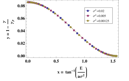
Figure 5: (Color online) Three groups of data fall on a single line with our choice of $y$ and $x$. Eq.(12) coincides well with the numerical data in this figure

In Fig. 5 all points collapse onto a single curve. We should mention that Eq. (12) only includes the main correction from $E/\sigma^{2}$. There are higher order corrections in $f(E/\sigma^{2})$ [12]. The small deviation between Eq. (12) and the numerical data was shown in Fig. 6.

At $x=0$ point, where $E=0$, it is already known that Eq. (2) is only valid in weak disorder limit. $\gamma$ behaves in logarithmic of the disorder strength in strong disorder limit, and the crossover curve between the two limits can be found in Ref. [11]. The difference around $x=0$ point is reasonable: $\sigma^{2}=0.02$ is not weak enough and higher order corrections of the perturbation in $\sigma^{2}$ becomes apparent. In the weak disorder limit ($\sigma^{2}=0.005,0.00125$ in Fig. 6) all the curves for different $\sigma^{2}$ is a single curve, which depends on $E/\sigma^{2}$ only.

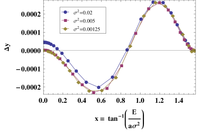
Figure 6: (Color online) The difference between the numerical data and Eq. (12).

4 Conclusion

In summary, we calculated the inverse localization length in one-dimensional Anderson model with diagonal disorder. We obtained numerically the curve of the inverse localization length for energies inside the energy band in the case of weak disorder. A unifying curve was given for different weak disorder strengths and energies outside the band edge anomalous region.

The scaled energy used to plot the unifying curve is $E/\sigma^{2}$, which has correspondence to the scaling parameter $\kappa=l_{loc}/l_{s}$ proposed by Deych et al. [7]. They used $\kappa$ for the criterion of SPS, which has a clear physical image. However, the new length scale $l_{s}$ and the localization length $l_{loc}$ are both functions of the energy $E$ and the disorder strength $\sigma^{2}$. Thus $\kappa$ is a two parameter function $\kappa(E,\sigma^{2})$. And we showed in this work that $\kappa$ actually depends on the single parameter $E/\sigma^{2}$, which is the essential parameter to give the universal curve in Fig. 5.

We also found a similar unifying description of the perturbation theory and the band center anomaly for the box distribution of disorder. We believe that other kinds of uncorrelated disorder with a finite variance can have the same unifying description. It should be mentioned that the Lorentzian distribution has no such band center anomaly, because its variance does not exist.

5 Acknowledgments

This work was supported by National Natural Science Foundation of China No. 10374093, the National Program for Basic Research of MOST of China, and the Knowledge Innovation Project of Chinese Academy of Sciences.

References

- Abrahams et al. [1979] Abrahams, E., Anderson, P.W., Licciardello, D.C., Ramakrishnan, T.V., 1979. Phys. Rev. Lett. 42, 673.
- Anderson [1958] Anderson, P.W., 1958. Phys. Rev. 109, 1492.
- Anderson et al. [1980] Anderson, P.W., Thouless, D.J., Abrahams, E., Fisher, D., 1980. Phys. Rev. B 3519, 22.
- Barnes and Luck [1990] Barnes, C., Luck, J.M., 1990. J. Phys. A-Math. Gen. 23, 1717.
- Derrida and Gardner [1984] Derrida, B., Gardner, E., 1984. J. Physique 45, 1283.
- Deych et al. [2003a] Deych, L.I., Erementchouk, M.V., Lisyansky, A.A., 2003a. Phys. Rev. Lett. 90, 126601.
- Deych et al. [2003b] Deych, L.I., Erementchouk, M.V., Lisyansky, A.A., Altshuler, B.L., 2003b. Phys. Rev. Lett. 91, 096601.
- Deych et al. [2001] Deych, L.I., Lisyansky, A.A., Altshuler, B.L., 2001. Phys. Rev. B 64, 224202.
- Evers and Mirlin [2008] Evers, F., Mirlin, A., 2008. Rev. Mod. Phys. 80, 1355.
- Izrailev et al. [1998] Izrailev, F.M., Ruffo, S., Tessieri, L., 1998. J. Phys. A-Math. Gen. 31, 5263.
- Kang et al. [2010] Kang, K., Qin, S.J., Wang, C.L., 2010. Commun. Theor. Phys. 54, 735.
- Kappus and Wegner [1981] Kappus, M., Wegner, F., 1981. Z. Phys. B 45, 15.
- Kaya [2009] Kaya, T., 2009. Eur. Phys. J. B 67, 225.
- Kramer and Mackinnon [1993] Kramer, B., Mackinnon, A., 1993. Reports on Progress in Physics 56, 1469.
- Lagendijk et al. [2009] Lagendijk, A., Bart, v.T., Wiersma, D.S., 2009. Phys. Today 62, 24.
- Lee and Stone [1985] Lee, P.A., Stone, A.D., 1985. Phys. Rev. Lett. 55, 1622.
- Lifshitz et al. [1988] Lifshitz, I.M., Gredeskul, S.A., Pastur, L.A., 1988. Introduction to the Theory of Disordered Systems. Wiley, New York.
- Pendry [1994] Pendry, J.B., 1994. Adv. in Phys. 43, 461.
- Ryu et al. [2004] Ryu, S., Mudry, C., Furusaki, A., 2004. Phys. Rev. B 70, 195329.
- Schmitteckert et al. [1998] Schmitteckert, P., Schulze, T., Schuster, C., Schwab, P., Echern, U., 1998. Phys. Rev. Lett. 80, 560.
- Schomerus and Titov [2002] Schomerus, H., Titov, M., 2002. Phys. Rev. E 66, 066207.
- Schomerus and Titov [2003] Schomerus, H., Titov, M., 2003. Phys. Rev. B 67, 100201.
- Stone et al. [1983] Stone, A.D., Allan, D.C., Joannopoulos, J.D., 1983. Phys. Rev. B 27, 836.
- Thouless [1979] Thouless, D.J., 1979. Ill-condensed Matter. Amsterdam, North-Holland.
- Yang et al. [2009] Yang, L.P., Wang, Y.J., Xu, W.H., Qin, M.P., Xiang, T., 2009. J. Phys: Condens. Matter 21, 145407.