Phase behaviour of polydisperse spheres: simulation strategies and an application to the freezing transition

Abstract

The statistical mechanics of phase transitions in dense systems of polydisperse particles presents distinctive challenges to computer simulation and analytical theory alike. The core difficulty, namely dealing correctly with particle size fractionation between coexisting phases, is set out in the context of a critique of previous simulation work on such systems. Specialized Monte Carlo simulation techniques and moment free energy method calculations, capable of treating fractionation exactly, are then described and deployed to study the fluid-solid transition of an assembly of repulsive spherical particles described by a top-hat “parent” distribution of particle sizes. The cloud curve delineating the solid-fluid coexistence region is mapped as a function of the degree of polydispersity $\delta$, and the properties of the incipient “shadow” phases are presented. The coexistence region is found to shift to higher densities as $\delta$ increases, but does not exhibit the sharp narrowing predicted by many theories and some simulations.

I Introduction

A complex fluid is described as “polydisperse” when its constituent particles are not all identical, but exhibit a spread of size, shape or charge. Polydispersity is a pervasive feature of both natural and synthetic macromolecular systems such as colloids, polymers and liquid crystals. But for many years it was regarded as a practical and conceptual nuisance to be minimised in experiment and ignored by theory. More recently, however, it has become clear that polydispersity is actually a matter of fundamental interest and practical importance in its own right, giving rise as it does to a rich variety of phenomena not observed in monodisperse systems (for a review, see SollichSollich (2002)). Examples include novel phase behaviour such as an extreme sensitivity of phase boundaries to the presence of rare large particles Wilding et al. (2005), critical points that occur below the maximum coexistence temperatureKita et al. (1997); Wilding et al. (2008), density dependent wetting transitions Buzzacchi et al. (2006) and surface size segregation effects Pagonabarraga et al. (2000); Buzzacchi et al. (2004), as well as interesting dynamical effects such as an enhanced propensity to glass formation Zaccarelli et al. (2009) and the possibility of multistage relaxation processes Warren (1999).

Despite the upsurge of interest in polydispersity induced phenomena in complex fluids, several basic questions remain. A prime example is the nature of the freezing transition for simple spherical particles with a spread of diameters, which in quantitative terms is conveniently characterized by a parameter $\delta$ measuring the standard deviation of the diameter distribution in units of its mean. Intuitively one expects that polydispersity should alter the location of the freezing curve and destabilize crystalline phases Pusey (1987). However, the character and extent of these alterations remain unclear despite extensive study by experiment Pusey and Megen (1986); Pusey (1991), density functional theories Barrat, J.L. and Hansen, J.P. (1986); McRae and Haymet (1988), simplified analytical theories Phan et al. (1998); Pusey (1987); Bartlett (1997); Sear (1998); Bartlett and Warren (1999); Xu and Baus (2003) and simulation Dickinson et al. (1981); Dickinson and Parker (1985); Stapleton et al. (1990); Bolhuis and Kofke (1996); Kofke and Bolhuis (1999); Lacks and Wienhoff (1999); Huang and Xu (2004); Fernandez et al. (2007); Yiannourakou et al. (2009); Yang and Ma (2009); Fernández et al. (2010); Nogawa et al. (2010, ). On the experimental side there is evidence for a ”terminal” degree of polydispersity $\delta_{t}$ above which a fluid will not crystallize. This is supported by a number of theoretical and simulation studies, some of which suggest that the terminal polydispersity arises from a progressive narrowing of the fluid-solid coexistence region with increasing $\delta$, with the boundaries of this region meeting at a point of equal concentration Phan et al. (1998); Bartlett and Warren (1999); Huang and Xu (2004); Nogawa et al. (2010, ). A reentrant melting scenario has also been proposed whereby compressing a crystal with a polydispersity slightly below $\delta_{t}$ can cause it to meltBartlett and Warren (1999). One simulation study predicts the occurrence of a partly crystalline “inhomogeneous phase” Fernandez et al. (2007) at high polydispersity, while other work has argued that the suppression of crystallization is a dynamical effect arising variously from the low diffusivity of large particles Evans and Holmes (2001), the intervention of a glass transition Pusey and van Megen (1987); Chaudhuri et al. (2005); Fernández et al. (2010), or anomalously large nucleation barriers Auer and Frenkel (2001).

In our view, the reason for the diverse predictions of theory and simulation regarding the equilibrium phase behaviour is that much previous theoretical and simulation work has failed to cater properly for a key feature of polydisperse phase equilibria, namely fractionation – the phenomenon whereby the distribution of particle sizes can be different among coexisting phases, whilst the overall distribution (across all phases) is fixed. One approach that does incorporate fractionation exactly (within the context of a mean field theory) is the moment free energy (MFE) method. Previous MFE calculations by one of us Fasolo and Sollich (2003, 2004) find neither evidence for narrowing of the coexistence region with increasing $\delta$, nor reentrant melting. Instead they predict that a polydisperse fluid can always split off a small amount of a solid phase having a narrow distribution of particle sizes. The purpose of the present paper is to compare the findings of MFE calculations with the results of tailored Monte Carlo (MC) simulations that similarly cater exactly for fractionation effects.

The paper is arranged as follows. In Sec. II we outline principal aspects of the phenomenology of polydisperse phase equilibria. We then present in Sec. III a detailed discussion of general issues surrounding the best choice of simulation ensemble for obtaining accurate estimates of phase coexistence properties. Sec. IV describes the model system we have studied and the bespoke techniques we have developed to determine fluid-solid coexistence properties. The results of applying these techniques to polydisperse spheres are described in Sec. V. Sec. VI summarizes our conclusions.

II Phenomenology of polydisperse phase equilibria

Typically one describes the polydispersity of a given system in terms of a density distribution $\rho^{(0)}(\sigma)$ which counts the number of particles per unit volume whose value of the polydisperse attribute $\sigma$, lies in the range $\sigma\dots\sigma+d\sigma$ Salacuse and Stell (1982). In most real polydisperse systems the form of $\rho^{(0)}(\sigma)$ is fixed by the synthesis of the fluid, and only its scale can change according to the degree of dilution of the system. Accordingly, one writes

$$\rho^{(0)}(\sigma)=n^{(0)}f(\sigma)$$ (1)

where $f(\sigma)$ is a normalized fixed shape function and $n^{(0)}$ is the overall number density. Varying $n^{(0)}$ corresponds to scanning a “dilution line” of the system.

At coexistence, particles with different $\sigma$ values will be partitioned unequally between the phases. This is the phenomenon of “fractionation”. To describe it, it is necessary to define separate “daughter” density distributions $\rho^{(\gamma)}(\sigma)$ ($\gamma=1,2,\ldots$) which measure the distribution of the polydisperse attribute for each phase $\gamma$. When the polydispersity is fixed, particle conservation implies that the weighted average of the daughter distributions equals the fixed overall density distribution, or “parent” $\rho^{(0)}(\sigma)$, i.e.

$$\rho^{(0)}(\sigma)=n^{(0)}f(\sigma)=\sum_{\gamma}\xi^{(\gamma)}\rho^{(\gamma)}(\sigma),$$ (2)

with $\xi^{(\gamma)}$ the fractional volume of phase $\gamma$, where $\sum_{\gamma}\xi^{(\gamma)}=1$. This expression represents a generalisation of the lever rule to polydisperse systems.

To illustrate the profound differences between phase behaviour in monodisperse and polydisperse systems, it is instructive to recall first the familiar case of the binodal curve of a monodisperse system in the density-temperature plane. This curve serves a dual purpose: on the one hand it describes the range of overall densities for which phase coexistence occurs; and on the other hand it identifies the densities of the coexisting phases themselves. Now, for a polydisperse system the range of overall (parent) densities that leads to coexistence is similarly delineated by a curve in $n^{(0)}$-temperature space – the so-called “cloud” curve. However, the densities of the coexisting phases themselves do not in general coincide with the cloud curve. Instead, as one varies the parent density $n^{(0)}$ through the coexistence region at a fixed temperature (say), one generates an infinite sequence of pairs of differently fractionated coexisting phases.

Insight into this phenomenology can be gained by considering the simplest case of a bidisperse (binary) mixture with densities $\rho_{1}$ and $\rho_{2}$ of two species of particles of different sizes; these are the analog of $\rho^{(0)}(\sigma)$. Fig. 1 sketches an isothermal cut through an exemplary bulk phase diagram, showing a region of fluid-fluid phase separation with tie-lines that shrink to zero at a critical point (c.p.). The dilution line constraint of a fixed shape for $\rho^{(0)}(\sigma)$ reduces in the bidisperse case to a fixed ratio $\rho^{(0)}_{1}/\rho^{(0)}_{2}$ (indicated by the dashed line in Fig. 1). As $n^{(0)}=\rho^{(0)}_{1}+\rho^{(0)}_{2}$ is increased from zero, the system follows the dilution line into the coexistence region, which it enters (and leaves) at a “cloud point”. For a given point on the dilution line inside the coexistence region, the parent splits into two daughter phases located at the ends of the tie-line which intersects this point. However, owing to fractionation, the daughters lie off the dilution line.

Figure 1: Schematic of an isothermal cut through the fluid-fluid phase diagram of the binary mixture described in the text. Thick solid line: coexistence boundary; thin solid lines: tie-lines; dashed line: dilution line, here chosen as $\rho^{(0)}_{1}=\rho^{(0)}_{2}$.

Since an infinite number of points occupy the dilution line between the cloud points, an infinite sequence of differently fractionated coexisting states is encountered as the coexistence region is traversed. Customarily one singles out the end points of this sequence for special attention, i.e. the case of incipient phase separation that occurs when the value of $n^{(0)}$ coincides with one of the two cloud points. Under these conditions, one daughter phase has a fractional volume of essentially unity and consequently (from the lever rule, Eq. (2)) a density distribution that is identical to the parent, while the other phase – known as the “shadow” – has an infinitesimal fractional volume and a density distribution that deviates maximally from that of the parent. The curve formed by plotting the number density (or packing fraction) of the shadow phase as a function of temperature is known as the shadow curve.

Qualitative differences between the phase behaviour of monodisperse and polydisperse systems are also evident in other projections of the full phase diagram. For instance, in the pressure-temperature plane, coexistence for a monodisperse system occurs along a line. By contrast for a polydisperse system, coexistence occurs within a region of the pressure-temperature phase diagram Rascon and Cates (2003); Bellier-Castella et al. (2000). This is because each of the infinite sequence of coexisting states along the dilution lines is associated with a different pressure, and so the pressure varies as one crosses the coexistence region. For a fuller account of the phenomenology of phase behaviour in polydisperse fluids, we refer the reader to a previous review Sollich (2002).

III Simulation strategies for polydisperse systems

Computer simulation is a principal route to determining the phase behaviour of model thermal systems, and many such investigations of polydisperse systems have been reported. Dickinson et al. (1981); Dickinson and Parker (1985); Stapleton et al. (1990); Bolhuis and Kofke (1996); Kofke and Bolhuis (1999); Lacks and Wienhoff (1999); Huang and Xu (2004); Fernandez et al. (2007); Yiannourakou et al. (2009); Yang and Ma (2009); Fernández et al. (2010); Nogawa et al. (2010, ) However the results that have emerged from the various studies are generally much more at variance with one another (even for a given model) than is typically the case in comparable studies of monodisperse systems. It therefore seems appropriate to consider carefully what particular issues and challenges polydispersity presents for simulation and how best to tackle them in practice. To this end we provide here a detailed critical assessment of the relative utility of the various statistical ensembles and simulation strategies that have been employed previously for the computational study of phase transitions in polydisperse systems. Our discussion distinguishes two categories of ensemble: those that fully permit density fluctuations at the level of individual particle species (“unconstrained density ensembles”), and those (“constrained density ensembles”) that do not. We argue that the latter category are seriously deficient both with regard to their ability to probe equilibrium phase behaviour, and their susceptibility to finite size effects. By contrast, unconstrained density ensembles – whilst requiring some effort to fully realize their benefits – constitute the method of choice for accurate studies of polydisperse phase equilibria.

III.1 Unconstrained densities

As is now well established Wilding (1995); Panagiotopoulos (2000), an efficient and accurate strategy for determining phase boundaries in monodisperse systems is to employ an ensemble that captures on a global scale the fluctuations characteristic of the transition. Prime examples are the grand canonical ensemble (constant $\mu,V,T$) and the isobaric-isothermal ensemble (constant $N,p,T$) Frenkel and Smit (2002). The common feature of these ensembles is that they avoid physical contact (i.e. interfaces) between coexisting phases even when operating at a coexistence state point. Instead the two phases are linked – and their relative free energies measured – via a phase space path Bruce and Wilding (2003) (the negotiation of which may entail biased sampling) that permits the simulation to fluctuate back and forth between the disjoint configuration spaces of the pure phase states. Although this path may traverse mixed phase (i.e. interfacial) states en-route between the pure phases, the associated surface tension penalty is such that at any one time, the system will be found with overwhelming probability in pure phase states. Accordingly there is ample opportunity to sample the properties of the phases whilst they occupy the maximum available system volume – thus minimizing finite-size effects. Indeed it has been shown that when the system is found with equal probability in each phase (the “equal weight criterion”), finite-size corrections to measured coexistence properties are exponentially small in the system size Borgs and Kotecky (1992).

In seeking to study phase behaviour in polydisperse systems, it is clearly desirable to retain the aforementioned benefits of the ($\mu,V,T$) and ($N,p,T$) ensembles, whilst at the same time generalizing them to permit sampling of the fluctuations in the polydisperse attribute. More specifically, one wishes to cater for fractionation so that the distribution of $\sigma$ (which for definiteness we shall take as the particle size) can vary from phase to phase. For the particular case of MC simulations within the ($\mu,V,T$) ensemble, the total particle number fluctuates (by means of insertions and deletions) and incorporating polydispersity entails imposing a distribution of chemical potentials $\mu(\sigma)$ and additionally introducing particle resizing updates. Doing so permits fluctuations not only in the overall instantaneous size distribution $\rho(\sigma)$, but also in the daughter distributions, thus facilitating efficient relaxations to a fractionated state.

However, to tackle the experimentally relevant scenario of fixed polydispersity, one further needs to ensure that the ensemble averaged density distribution (across all coexisting phases) corresponds to some prescribed parent as expressed in Eq. (2). To do so entails solving an inverse problem for $\mu(\sigma)$ Wilding and Sollich (2002); Wilding (2003), a task which – at first sight – appears complicated by the fact that each phase will (in general) either be absent or occupy the whole simulation box rather than its true canonical fractional volume $\xi^{(\gamma)}$. Fortunately, a straightforward solution has been developed by Buzzacchi et al. in which $\mu(\sigma)$ and the $\xi^{(\gamma)}$ are treated as parameters which are tuned iteratively such as to simultaneously satisfy an equal weight criterion for the coexisting phases and the lever rule constraint Buzzacchi et al. (2006). This technique permits the determination of coexistence properties with finite size effects that are exponentially small in the box size, even in the limit in which one of the phases has an infinitesimal fractional volume.

Whilst appropriate for studying fluid phase transitions in polydisperse systems, the ($\mu(\sigma),V,T$) ensemble is unsuitable in situations where one or more of the coexisting phases is a crystalline solid because the number density of a crystal cannot easily fluctuate without engendering defects. Instead it is advantageous to appeal to a hybrid of the grand canonical and $(N,p,T)$ ensembles known as the isobaric-semi-grand canonical ensemble (SGCE) Kofke and Glandt (1987); Frenkel and Smit (2002). This is the analog of a monodisperse $(N,p,T)$ ensemble where the particle number is fixed but the prevalence of the various particle sizes is controlled by imposing chemical potential differences $\tilde{\mu}(\sigma)$ that are measured relative to the chemical potential of some reference particle size. The SGCE has been widely deployed in the simulation of fluid mixtures Frenkel and Smit (2002) and was first applied to polydisperse systems by Kofke and Glandt Kofke and Glandt (1987). Although the overall particle number is fixed in the SGCE, via the constraint $V\int\rho(\sigma)d\sigma=N$, particle size updates nevertheless permit the sampling of many realizations of the polydisperse disorder, while updates of the overall volume allow the total system number density to relax in each phase. Thus the ensemble provides as many degrees of freedom vis a vis density fluctuations as the $(\mu(\sigma),V,T$) ensemble and hence permits efficient treatment of fractionation. An additional attractive feature of the SGCE is that it provides direct access to the coexistence pressure which is not the case in the $(\mu(\sigma),V,T$) ensemble. In Sec. IV.4 we shall describe how to combine the SGCE with the method of Buzzacchi et al. Buzzacchi et al. (2006) to permit accurate determination of coexistence properties of polydisperse systems.

III.2 Constrained densities

We now consider the comparative utility of other ensembles that have been utilized in the study of polydisperse phase equilibria, but which constrain the particle densities to a greater or lesser degree. These are the microcanonical ($N,V,E$) Fernández et al. (2010), canonical ($N,V,T$) Fernandez et al. (2007) and isobaric-isothermal ($N,p,T$) Nogawa et al. (2010) ensembles. We focus first on the fully constrained ($N,V,T$) and ($N,V,E$) ensembles. Here two or more extensive quantities are conserved and consequently at coexistence the simulation box divides into separate regions, each occupied by one phase which is connected by an interface to its neighbour. As a result, measurements of the properties of one phase can be affected by the presence of the interface with the other phase. Whilst in a monodisperse system – where the properties of the two coexisting phases are independent of their fractional volumes in the thermodynamic limit – one can mitigate interfacial effects by measuring the properties at equal fractional volumes, i.e. $\xi^{(1)}=\xi^{(2)}=1/2$, the situation is much more delicate for polydispersity. Here, owing to fractionation, the character of the phases depends inherently on their fractional volume, and accordingly their properties need to be determined even when one of the phases occupies a small fractional volume. However, in a finite-sized system, this generally translates to a small absolute volume, and thus the properties of such a phase will unavoidably be dominated by its interface. This effectively precludes the accurate determination of bulk properties in these ensembles. In particular, near cloud points the corresponding shadow phases may occupy too small a volume to form at all, because of interfacial free energy costs, and this can lead to serious misestimates of cloud point locations.

Finite size effects are further exacerbated in the ($N,V,E$), ($N,V,T$) and indeed the ($N,p,T$) ensembles by the fact that polydispersity is incorporated by assigning each of the $N$ particles a fixed size drawn from the prescribed parent distribution. Consequently only a single realization of the parent is considered rather than a fluctuating sample as occurs in the ($\mu(\sigma),V,T$) or SGCE approaches. Fixed particle sizes represent a particular handicap in the interface-forming ($N,V,E$) and ($N,V,T$) ensembles when fractionation effects are strong, so that e.g. one daughter phase has a distribution that is strongly peaked towards the largest particles Speranza and Sollich (2003); Fasolo and Sollich (2004). If in that particle size range the parent density is low, then the lever rule forces the relevant daughter phase to have a small fractional volume and hence also small absolute volume, with the problematic consequences discussed above. Equally if not more importantly, the sampling of the size distribution with $N$ particles of fixed size may be too coarse to represent such sharply peaked daughter distributions accurately, especially in a tail region of the parent. This causes deviations from thermodynamic bulk behaviour that cannot be corrected in any straightforward way.

A further practical disadvantage of fixed particle sizes is that for dense systems where diffusion is inhibited, particles of a given size may not reach their favored phase on simulation timescales. Whilst in MC implementations this can be overcome by employing long ranged particle moves or particle exchanges Fernandez et al. (2007), it effectively prevents relaxation in molecular dynamics (MD) simulations which employ realistic dynamics. A case in point is the recent work of Nogawa et al. Nogawa et al. (2010), who performed MD in an ($N,p,T$) ensemble to simulate a system of size-disperse spheres initialized in an interfacial state of coexisting fluid and solid phases. As discussed above, interfacial configurations are disfavored over pure phase states in the ($N,p,T$) ensemble. But once initialized, an interface can nevertheless be maintained for a substantial period if the prescribed pressure is carefully tuned such that the interface is stationary (neither grows nor shrinks on average). This pressure serves – in principle – as a measure of the coexistence pressure. However, because in the study of Nogawa et al. the size distribution was initialized to be identical in both phases, and since no significant fractionation of the phases occurred on simulation timescales, the results emerging from this study cannot be regarded as representative of equilibrium.

Further evidence for the disadvantages of employing constrained density ensembles is to be found in the recent work of Fernandez and co-workers Fernandez et al. (2007); Fernández et al. (2010) who employed ($N,V,E$) and ($N,V,T$) MC simulations to study the fluid-solid coexistence of polydisperse soft spheres. In these ensembles, an interface between coexisting phases is mandated to form in the thermodynamic limit, as pointed out above. Apparently, however, none was observed at small degrees of polydispersity, with the system simply fluctuating between the pure phases – a feature which presumably reflects the rather small system size used. Only at high degrees of polydispersity did an interface form, but the authors interpreted its appearance as a polydispersity induced “inhomogeneous phase” rather than an essential feature of their choice of ensemble. Even in this region of apparent phase separation, no account was taken of the finite width of the coexistence region, i.e. no attempt was made to distinguish the infinity of coexistence curves, or even the boundary of the coexistence region, either in density or temperature space. This presumably reflects the difficulties of dealing correctly with situations where one phase is incipient, as described above. Although use of long range particle exchange moves resulted in some evidence for fractionation well inside the coexistence region, it is our view that the results emerging from Refs. Fernandez et al. (2007); Fernández et al. (2010) are nevertheless qualitatively unreliable. Indeed it was this conviction that catalysed the present study, in which we revisit the phase diagram of the same model studied by Fernandez and co-workers, but using the SGCE and specialized data analysis techniques in order to extract the correct phase behaviour.

III.3 Fixed versus variable parent

As discussed in Sec. II, in many complex fluids such as colloids and polymers, the form of the polydispersity is determined by the process of chemical synthesis and hence the shape of the parent density distribution is fixed. The phase behaviour is then as described in Sec. II. However, most previous computational studies that use the SGCE or ($\mu,V,T)$ ensemble to facilitate fractionation have not sought to adapt the form of $\tilde{\mu}(\sigma)$ in order to ensure that the ensemble averaged density distribution $\bar{\rho}(\sigma)$ had a fixed functional form, corresponding to a prescribed parental size distribution $f(\sigma)$.Stapleton et al. (1990); Bolhuis and Kofke (1996); Kofke and Bolhuis (1999); Yiannourakou et al. (2009); Yang and Ma (2009) Instead the activity distribution $\exp[\beta\tilde{\mu}(\sigma)]$ was assigned a fixed form such as a Gaussian, peaked at some $\sigma_{0}$, and various widths of the Gaussian were used in order to change the degree of polydispersity.

In such a fixed chemical potential approach, $\bar{\rho}(\sigma)$ can vary dramatically across the phase diagram with the result that one doesn’t capture the phase behaviour of a particular parent form as would be the case experimentally. Moreover, many of the characteristic features of phase coexistence for a fixed parent are absent. Specifically, when crossing a coexistence region at fixed chemical potentials, the system follows a tie line rather than cutting an infinity of tie lines as occurs when the dilution line constraint (Eq. 1) is imposed. This difference is then manifest in the fact that coexistence occurs only along a line in the $(T,p)$ plane for fixed chemical potentials, rather than within a region. Such features are more akin to those occuring in a monodisperse system and accordingly the fixed chemical potential approach misses much of the essential phenomenology of experimental systems, a fact that severely limits its applicability.

III.4 Summary

We conclude this section by distilling the salient points of the above commentary. The central message is that in computational studies of phase behaviour in dense polydisperse systems, the choice of simulation ensemble can have far greater implications for the severity of finite-size effects and the pace of relaxation than in monodisperse systems. Specifically, we believe that despite the fact that they ostensibly offer a simple route to fixing the parent form, polydisperse versions of the ($N,V,E$) and ($N,V,T$) ensembles are to be avoided. This is because on the one hand they are intrinsically hamstrung by serious finite-size effects (whose origin lies in interface formation), and on the other hand they can suffer from very long relaxation times.

Suitable ensembles for dealing with a fixed parent are the $(\mu(\sigma),V,T)$ ensemble and the SGCE, the latter being most appropriate when solid phases are involved. Their strengths are two-fold, namely that they: (i) permit estimates of coexistence properties with finite-size corrections that are exponentially small in the system size, even in the limit where one of the phases has an infinitesimal fractional volume; and (ii) accelerate fractionation via particle size updates that circumvent the physical diffusion process. The (modest) price to be paid in order to realize these benefits is the need to determine at each state point of interest a chemical potential distribution and values for the fractional phase volumes $\xi^{(\gamma)}$. These must simultaneously satisfy the lever rule and an equal weight criterion. In Sec. IV.4 we describe how this can be efficiently achieved within the context of the SGCE.

IV Models and Methodologies

IV.1 Models

The systems that we shall consider in this work are assemblies of spheres interacting either by a repulsive soft sphere potential (as considered by simulation) or a hard sphere potential (as studied in our moment free energy method calculations). The soft sphere interaction potential between two particles $i$ and $j$ with position vectors $\bm{r}_{i}$ and $\bm{r}_{j}$ and diameters $\sigma_{i}$ and $\sigma_{j}$ is given by

$$v(r_{ij})=\epsilon(\sigma_{ij}/r_{ij})^{12}\>,$$ (3)

with particle separation $r_{ij}=|\bm{r}_{i}-\bm{r}_{j}|$ and interaction radius $\sigma_{ij}=(\sigma_{i}+\sigma_{j})/2$. The choice of this potential rather than hard spheres is made on pragmatic grounds; in our isobaric SGCE simulations (to be reported below), any MC contraction of the simulation box that leads to an infinitesimal overlap of two hard spheres will always be rejected, so (particularly at high densities) we can expect higher MC acceptance rates using this “softer” potential. In common with hard spheres, the monodisperse version of our model freezes into an fcc crystalline structure Hansen (1970); Hoover et al. (1970); Wilding (2009), and temperature only plays the role of a scale: the thermodynamic state depends not on $n^{(0)}$ and $T$ separately but only on the combination $n^{(0)}(\epsilon/k_{\mathrm{B}}T)^{1/4}$. Phase diagrams for different $T$ then scale exactly onto one another, and we can fix $\epsilon/k_{\mathrm{B}}T=1$.

In all cases we consider parent size distributions of the top-hat form:

$$f(\sigma)=\left\{\begin{array}[]{ll}(2c)^{-1}&\mbox{ if $1-c\leq\sigma\leq 1+c$}\\ ~{}~{}0&\mbox{ otherwise }\end{array}\right..$$ (4)

Here the width parameter $c$ controls the degree of polydispersity $\delta=c/\sqrt{3}$, and we have set the mean particle diameter to 1. With these choices, and the interaction potential (3), our results are directly comparable to the phase diagram of Fernandez et al.Fernandez et al. (2007), bearing in mind that in the latter work neither fractionation nor, at a more basic level, the presence of coexistence regions of finite width was allowed for.

IV.2 The isobaric semi-grand canonical ensemble

Our simulations operate within the SGCE, wherein the particle number $N$, pressure $p$, temperature $T$, and a distribution of chemical potential differences $\tilde{\mu}(\sigma)$ are all prescribed, while the system volume $V$, the energy, and the form of the instantaneous density distribution $\rho(\sigma)$ all fluctuate Kofke and Glandt (1988). As discussed above, this is important to allow for separation into differently fractionated phases.

Operationally, the sole difference between the isobaric, semi-grand-canonical ensemble and the $(N,p,T)$ ensemble Frenkel and Smit (2002) is that one implements MC updates that select a particle at random and attempt to change its diameter $\sigma$ by a random amount drawn from a zero-mean uniform distribution. This proposal is accepted or rejected with a Metropolis probability controlled by the change in the internal energy and the chemical potential Kofke and Glandt (1987):

$$p_{\rm acc}={\rm min}\left[1,\exp{(-\beta[\Delta\Phi+\tilde{\mu}(\sigma)-\tilde{\mu}(\sigma^{\prime})])}\right]\>,$$

where $\Delta\Phi$ is the internal energy change associated with the resizing operation.

IV.3 Phase Switch Monte Carlo

Phase Switch Monte Carlo (PSMC) is a general method for determining phase boundaries but is particularly useful for dealing with fluid-solid coexistence.Wilding and Bruce (2000) The basic idea is to employ a reversible phase space leap that connects the configuration space of the fluid to that of the solid. This allows sampling of the disjoint configuration spaces of the two phases in a single simulation run and hence direct estimation of their relative free energies. The method has been previously described in detail in the context of monodisperse systems McNeil-Watson and Wilding (2006), as has its extension to polydisperse systems.Wilding (2009) We therefore confine ourselves to providing only a bare outline here.

The method is based on a mapping between two reference configurations – one for the fluid and one for the solid. A reference configuration for a given phase $\gamma$ is simply an arbitrarily chosen configuration of that phase defined by the associated set of particle sites $\{\bm{R}\}^{\gamma}$. One can simply express the coordinates of each particle in phase $\gamma$ in terms of the displacement from its reference site, i.e.

$$\bm{r}^{\gamma}_{i}=\bm{R}^{\gamma}_{i}+\bm{u}_{i}\>.$$ (5)

Now, for displacement vectors that are sufficiently small in magnitude, one can clearly reversibly map any configuration $\{\bm{r}^{\gamma}\}$ of phase $\gamma$ onto a configuration of another phase $\gamma^{\prime}$ simply by switching the set of reference sites $\{\bm{R}\}^{\gamma}\to\{\bm{R}\}^{\gamma^{\prime}}$, while holding the set of displacements $\{\bm{u}\}$ constant. This switch, which forms the heart of the method, can be incorporated into a global MC move.

A complication arises, however, because the displacements $\{\bm{u}\}$ typical for phase $\gamma$ will not, in general, be typical for phase $\gamma^{\prime}$. Thus the switch operation will mainly propose high energy configurations of phase $\gamma^{\prime}$ which are unlikely to be accepted as a Metropolis update. This problem can be circumvented by employing biased sampling techniques to seek out those displacements $\{\bm{u}\}$ for which the switch operation is energetically favorable. These are the so-called gateway configurations, which typically correspond to displacement vectors that are small in magnitude.

Using the above formalism one can construct a sampling scheme which explores the configurations of high statistical weight in each phase, whilst returning at regular intervals to the low weight gateway configurations that permit a switch to the other phase. In this manner one can directly compare the relative statistical weights of the two phases and hence determine free energy differences and coexistence points.

IV.4 Fixing the parent distribution across coexisting phases and determining fractional volumes

For SGCE simulations of a polydisperse system at some given $N$ and $T$, we seek the pressure $p$ and distribution of chemical potential differences $\tilde{\mu}(\sigma)$ such that a suitably defined ensemble-averaged density distribution matches the prescribed parent $\rho^{(0)}(\sigma)=n^{(0)}f(\sigma)$. Unfortunately, the task of determining the requisite $p$ and $\tilde{\mu}(\sigma)$ is complicated by the fact they are unknown functionals of the parent Wilding (2003). To deal with this problem one can employ a version of a scheme originally proposed in the context of grand canonical ensemble studies of polydisperse phase coexistence Buzzacchi et al. (2006) and later extended to the SGCE Wilding (2009), the latter implementation of which we now summarize.

The strategy is as follows. For a given choice of $n^{(0)}$ and temperature $T$, one tunes $p$, $\tilde{\mu}(\sigma)$ and the $\xi^{(\gamma)}$ iteratively within a histogram reweighting (HR) framework Ferrenberg and Swendsen (1989), such as to simultaneously satisfy both a generalized lever rule and equality of the probabilities of occurrence of the phases, i.e.

$$n^{(0)}f^{(0)}(\sigma) = \sum_{\gamma}\xi^{(\gamma)}\rho^{(\gamma)}(\sigma),$$ (6a)

$${\mathcal{E}} = 0\>.$$ (6b)

In the first of these constraints, Eq. (6a), the ensemble averaged daughter density distributions $\rho^{(\gamma)}(\sigma)$ are assigned by averaging only over configurations belonging to the respective phase. The deviation of the weighted sum of the daughter distributions $\bar{\rho}(\sigma)\equiv\sum_{\gamma}\xi^{(\gamma)}\rho^{(\gamma)}(\sigma)$ from the target $n^{(0)}f^{(0)}(\sigma)$ is conveniently quantified by a ‘cost’ value:

$$\Delta\equiv\int\mid\bar{\rho}(\sigma)-n^{(0)}f^{(0)}(\sigma)\mid d\sigma\;.$$ (7)

In the second constraint, Eq. (6b),

$${\mathcal{E}}\equiv\sum_{\gamma}\left(p^{(\gamma)}-\frac{1}{n}\right)^{2}$$ (8)

provides a measure of the extent to which the probability of each phase occuring, $p^{(\gamma)}$, is equal for each of the $n$ coexisting phases. Imposing this equality ensures that finite-size errors in coexistence parameters are exponentially small in the system volume Borgs and Kotecky (1992); Buzzacchi et al. (2006).

The iterative determination of $p,\tilde{\mu}(\sigma)$ and $\xi^{(\gamma)}$ such as to satisfy Eqs. (6a) and (6b) proceeds thus:

1. Guess initial values of the fractional volumes $\xi^{(\gamma)}$ corresponding to the chosen value of $n^{(0)}$. Usually if one starts near a cloud point, the fractional volume of the incipient phase will be close to zero.

2. Tune the pressure $p$ (within the HR scheme) such as to minimize $\Delta$.

3. Similarly tune $\tilde{\mu}(\sigma)$ (within the HR scheme) such as to minimize $\Delta$.

4. Measure the corresponding value of ${\mathcal{E}}$.

5. if ${\mathcal{E}}<{\rm tolerance}$, finish, otherwise vary $\xi^{(\gamma)}$ (within the HR scheme) and repeat from step 2.

The minimization of $\Delta$ with respect to variations in $p$ (step $2$) can easily be automated using standard 1-dimensional minimization algorithms such as the “Brent” routine described in Numerical Recipes Press et al. (2007). Similarly we used the “Powell” routine for the multi-parameter minimization of ${\mathcal{E}}$ with respect to variations in $\xi^{(\gamma)}$ in step $5$. In step $3$ the minimization of $\Delta$ with respect to variations in $\tilde{\mu}(\sigma)$ is most readily achieved Wilding and Sollich (2002) using the following simple iterative scheme for $\tilde{\mu}(\sigma)$:

$$\tilde{\mu}_{k+1}(\sigma)=\tilde{\mu}_{k}(\sigma)+\alpha\ln\left(\frac{n^{(0)}f^{(0)}(\sigma)}{\bar{\rho}(\sigma)}\right)\;,$$ (9)

for iteration $k\to k+1$. This update is applied simultaneously to all entries in the histogram of $\tilde{\mu}(\sigma)$, and thereafter the distribution is shifted so that $\tilde{\mu}(\sigma_{0})=0$, where $\sigma_{0}$ is the chosen reference size. The quantity $0<\alpha<1$ appearing in Eq. (9) is a damping factor, the value of which may be tuned to optimize the rate of convergence.

The values of $\xi^{(\gamma)}$ and $p$ resulting from the application of the above procedure are the desired fractional volumes and pressure corresponding to the nominated value of $n^{(0)}$. As has been described previously Wilding (2009), daughter phase properties are obtainable by monitoring, separately for each phase, the density distribution $\rho^{(\gamma)}(\sigma)$ and the distribution of the fluctuations in the overall number density, $P(n)$, and the volume fraction, $P(\eta)$. Here the volume fraction is defined in the obvious way as $\eta=\int d\sigma\rho(\sigma)(\pi/6)\sigma^{3}$, for a phase with density distribution $\rho(\sigma)$.

IV.5 Analytical calculations: the moment free energy method

Calculating analytically the phase behaviour of polydisperse systems is a challenging problem Sollich (2002). This is because for each of the infinitely many different particle sizes $\sigma$ one has a separate conserved density $\rho(\sigma)$. Effectively one thus has to study the thermodynamics of an infinite mixture, where e.g. from the Gibbs rule there is no upper limit on the number of phases that can occur.

The moment free energy (MFE) method Sollich et al. (2001); Warren (1998); Sollich and Cates (1998); Sollich (2002) is designed to get around this issue by effectively projecting the infinite mixture problem down to that of a finite mixture of “quasi-species”. This is possible when the free energy density has a so-called truncatable form,

$$f=k_{\mathrm{B}}T\int d\sigma\rho(\sigma)\left[\ln(\rho(\sigma))-1\right]+f^{\rm ex}(\{\rho_{i}\})\ ,$$ (10)

where the excess part $f^{\rm ex}$ depends on a finite number of moments of the density distribution,

$$\rho_{i}=\int d\sigma\rho(\sigma)w_{i}(\sigma)\ .$$ (11)

This truncatable structure obtains for a large number of models of mean field type. Importantly for our purposes, it is also found in accurate free energy expressions for polydisperse hard spheres, with the simple weight functions $w_{i}(\sigma)=\sigma^{i}$ ($i=0,1,2,3$). Specifically, we use for the fluid the Boublik, Mansoori, Carnahan, Starling and Leland (BMCSL) expression Boublik (1970); Mansoori et al. (1971); Salacuse and Stell (1982) and for solid phases the free energy developed by Bartlett Bartlett (1997) on the basis of the simulation data of Kranendonk et al. Kranendonk and Frenkel (1991) for binary mixtures.

The MFE method is a way of expressing the ideal contribution to the free energy from Eq. (10), which depends on the complete shape of the density distribution, in terms of the moment densities $\rho_{i}$. The result is the moment free energy. The key feature of the method is that if one then treats the quasi-species densities $\rho_{i}$ as if they were densities of ordinary particle species, and calculates phase equilibria accordingly, the results for cloud and shadow points are fully exact. The MFE approach is therefore the method of choice for our current investigation. We do not give further details of the numerical implementation here as these are set out in full in Ref Fasolo and Sollich (2004).

V Fluid-solid coexistence

We have applied the simulation methodologies outlined in Secs. IV.2–IV.4 to determine the fluid-solid coexistence properties of the polydisperse soft sphere model. In parallel we have employed the MFE method outlined in Sec. IV.5 to determine the coexistence properties of polydisperse hard spheres. The reason for not using soft spheres also in the analytical calculations is that there are no sufficiently accurate free energy expressions available for this case. Qualitatively, however, we expect the hard and soft sphere systems to show similar behaviour, and will see that this is indeed the case.

Our simulations of the soft sphere model comprised systems of $N=256$ particles. The interparticle potential was truncated at half the box size and periodic boundary conditions were applied. Since for the system sizes studied the value of the potential is extremely small at the typical cutoff radius, no correction was applied for the truncation. As a preliminary step we determined the coexistence parameters of the transition from fluid ($F$) to face-centred-cubic (fcc) solid ($S$) in the monodisperse limit. This was done using the standard formulation of PSMC McNeil-Watson and Wilding (2006) with the results Wilding (2009): $p_{\rm coex}=22.32(3),\rho_{F}=1.148(9),\rho_{S}=1.190(9)$. Thereafter we attempted to locate the fluid phase cloud point ($\xi=0$) for a narrow top-hat parent having $c=0.01$. To this end we initialized the chemical potential difference distribution as $\tilde{\mu}(\sigma)=0$ (for $0.99\leq\sigma\leq 1.01$) and $\tilde{\mu}(\sigma)=-100$ otherwise, and assigned the pressure the value $p=22.32$ pertaining to the monodisperse limit. We then performed a long PSMC run, the results of which were reweighted (using the procedure described in Sec. IV.4 together with the monodisperse value $n^{(0)}=1.148$ as the initial guess for the fluid cloud point density), to yield accurate estimates of the fluid phase cloud point pressure, parent density $n^{(0)}$ and chemical potential difference distribution $\tilde{\mu}(\sigma)$, as well as the shadow phase daughter distribution.

In order to progress to higher degrees of polydispersity, we proceeded in a stepwise fashion. The form of $\tilde{\mu}(\sigma)$ previously determined for $c=0.01$ was extrapolated via a quadratic fit to cover the range $0.98\leq\sigma\leq 1.02$, while the pressure for $c=0.02$ was estimated by linearly extrapolating the results for $c=0.00$ and $c=0.01$. A new PSMC run was then performed, the results of which were reweighted to give accurate estimates of the cloud point parameters for the top hat parent with $c=0.02$. In this manner we were able to steadily increase the degree of polydispersity, measuring the fluid cloud point pressure and density as well as the corresponding solid shadow properties. In an identical fashion we determined the dependence on polydispersity of the solid cloud point parameters, by finding the value of $n^{(0)}$ for which $\xi=1$.

For values of $\delta>0.069$ on the solid cloud curve and $\delta>0.087$ on the fluid cloud curve, the system was found to make spontaneous transitions between the coexisting phases. Such an occurrence suggests a polydispersity induced lowering of the fluid-solid surface tension which normally provides the free energy barrier maintaining a simulation in the phase in which it is initiated. Unfortunately such spontaneous transitions undermine the phase switch strategy whereby one keeps track of the phase via the switch operation. Thus we were unable to reach larger values of the polydispersity than those quoted, but note that the values we can access are well within the range of typical experimental systems.

In seeking to compare the simulation and MFE results for phase coexistence properties, it is necessary to adopt a means of translating values of $\delta$ between soft and hard spheres. As standard mappings from soft to hard spheres fail at our densities, we use phase diagram topology to identify comparable points. This is achieved by scaling $\delta$ in order to match the location of certain phase transitions that occur in the solid region of the phase diagrams of our models Sollich and Wilding (2010) as will be described in detail elsewhere Sollich and Wilding . The scaling is linear and maps $\delta=0.088$ for soft spheres to $\delta=0.0546$ for hard spheres.

Our results for the cloud and shadow curves in the volume fraction-polydispersity plane are shown in Fig. 2. In this representation one sees a close accord between cloud and shadow curves. This is surprising given the presence of fractionation. But one can confirm by perturbation theory Sollich (2008); Evans (2001) that the behaviour we observe comes from the fact that in our models polydispersity enters only via the particle size and not the strength of the interaction. For the MFE results shown, symbols correspond to the scaled values of the polydispersity $\delta$ used in the simulations. Qualitatively the same behaviour is observed in this range. Quantitatively, the changes in volume fraction with the polydispersity $\delta$ are smaller than in the soft sphere system. For larger polydispersities, the existence of a terminal polydispersity beyond which a solid will be unstable manifests itself: the shadow solid curve never goes above $\delta\approx 0.06$ and bends down beyond this point. Cloud and shadow curves also begin to deviate from one another: the perturbative prediction that the curves should be identical for systems like the ones studied here applies only to the leading $O(\delta^{2})$ dependence of the volume fractions.

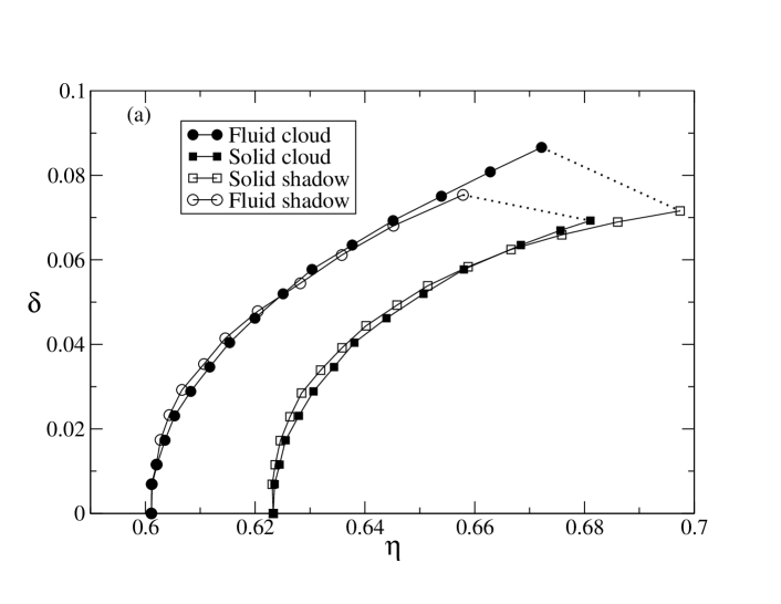
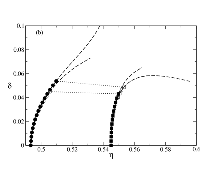
Figure 2: (a) Variation in the volume fraction of the cloud and shadow phases with their polydispersity at the freezing transition of soft spheres, Eq. (3), for the top-hat parent distribution, Eq. (4). (b) MFE calculation of cloud and shadow curves for hard spheres with the same parent form. The symbols shown are for the scaled analogues of the values of $\delta$ used in the simulations; dashed lines indicate MFE results beyond this range. Note that shadow phase volume fractions are plotted against their own $\delta$, not that of the parent. Dotted lines show exemplary tie lines connecting coexisting cloud-shadow pairs.

Much greater differences between cloud and shadow curves are apparent in the number density-vs-polydispersity representation (Fig. 3). Here we see that cloud and shadow curves separate strongly as polydispersity increases. Interestingly, the corresponding number density can then become less than that of the fluid shadow. This is a signature of fractionation: the fluid typically contains more of the smaller particles and the solid more of the larger ones as we will see below. As a consequence, a fluid phase can have higher density but lower volume fraction than a solid.

The same reasoning explains the relative position of the solid shadow and solid cloud curves. A solid at the cloud point has the parental size distribution while a solid shadow phase, which coexists with a cloud point liquid, has a different size distribution that contains more larger particles. Given that both have similar volume fractions as we saw above, the shadow solid must therefore have a smaller density than the cloud point solid. In the hard sphere case, this effect in fact outweighs the increase in cloud point volume fraction with $\delta$, so that the density of the shadow solid decreases rather than increases as $\delta$ increases from zero.

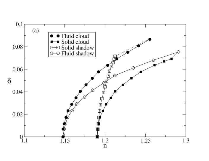
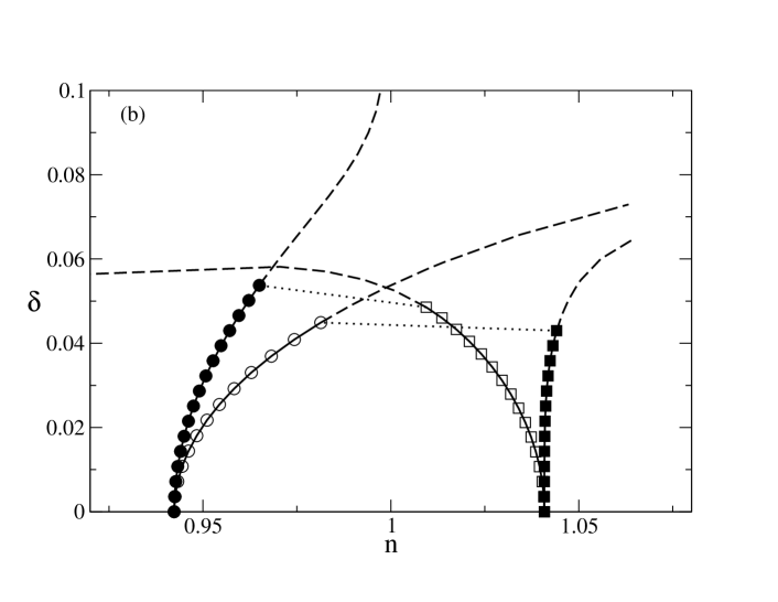
Figure 3: (a) Variation in the number densities of cloud and shadow phases with polydispersity at the freezing transition of soft spheres. (b) MFE calculation of cloud and shadow curves for hard spheres. The solid shadow curve is at lower densities than the solid cloud curve because the shadow solid phase contains more larger particles. For hard spheres the effect is so pronounced that the curve bends to the left. Dotted lines represent exemplary tie lines.

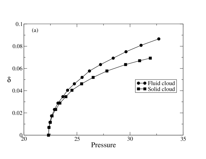
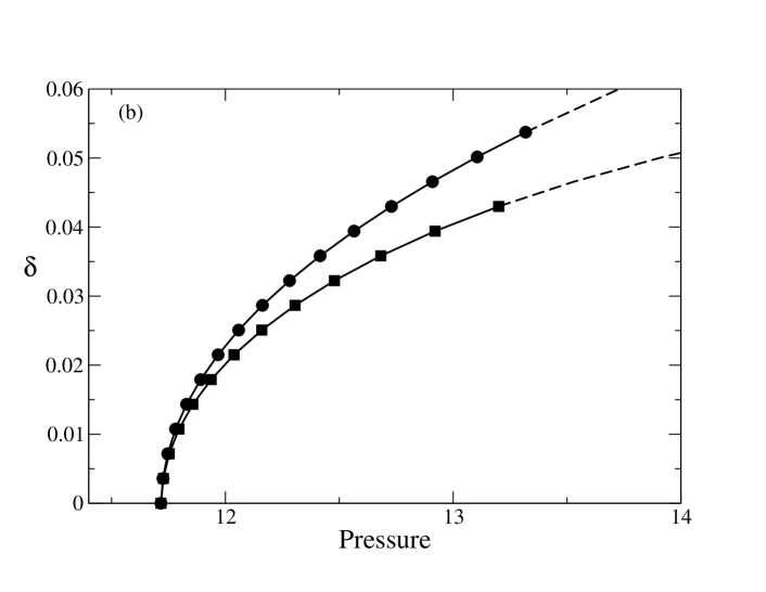
Figure 4: Polydispersity versus pressure at cloud points for (a) simulations of soft spheres, (b) MFE calculations for hard spheres.

Further evidence for fractionation is shown in Fig. 4, where we plot the cloud point pressures against the polydispersity of the parent. For a given $\delta$, fluid-solid coexistence occurs in the entire range between the two pressures shown: at the lowest pressure we are at the cloud point coming from the fluid side, where a small amount of shadow solid first appears; at the highest pressure we are at the solid cloud point, where there is only an infinitesimal amount of (shadow) liquid left.

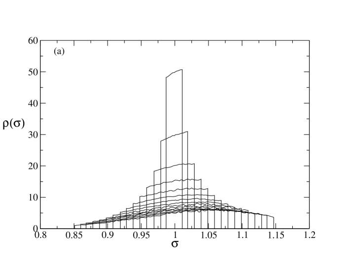
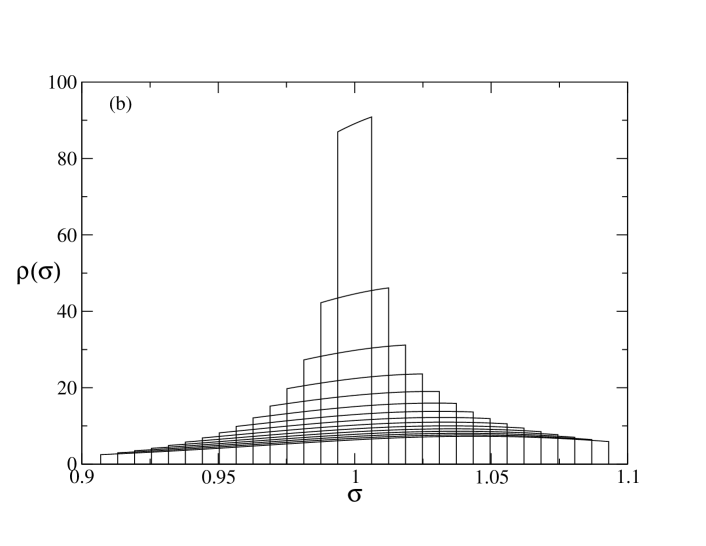
Figure 5: Density distribution in solid shadow phases for (a) simulations of soft spheres, (b) MFE calculations for hard spheres. The values of the parent $\delta$ used are scaled analogues of each other.

To understand the extent of fractionation in more detail, we consider in Figs. 5 and 6 the density distributions in the shadow phases. Both figures show excellent qualitative agreement between the results of the soft sphere simulations and the hard sphere MFE calculations. In Fig. 5 we plot the density distributions in the shadow solids, i.e. the solid phases that first form from the fluid as we increase the parent density. We observe the trend anticipated above: the distributions are generally increasing functions of $\sigma$, containing more of the larger particles than the coexisting fluids (which have the parental top-hat size distribution, given that we are at the fluid cloud point). A further aspect becomes apparent for larger parental $\delta$, where the shadow solid size distributions become narrower than the parent, being suppressed for both the smallest and the largest particle sizes. This reflects the fact that in a solid it is not possible to accommodate an arbitrarily large spread of particle sizes without destroying the crystalline order, which is at the origin of the existence of a terminal polydispersity for the solid.

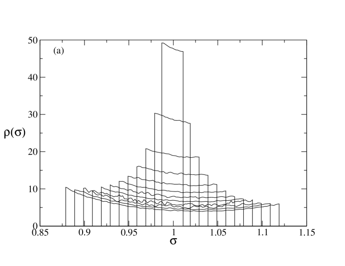
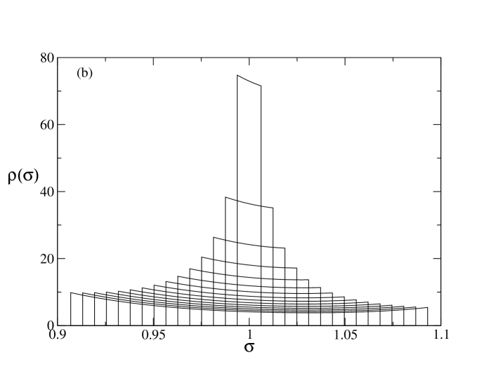
Figure 6: Density distribution in fluid shadow phases for (a) simulations of soft spheres, (b) MFE calculations for hard spheres.

The shadow fluid density distributions in Fig. 6 show, as might have been expected, that the opposite trends prevail in the fluid phases, i.e. the fluids that first appear when coming from high densities. These size distributions are generally biased towards smaller particles; for more strongly polydisperse parent distributions, they become enhanced towards the smallest and largest particle sizes, with a minimum in the middle. Both of these can be understood by extrapolation from within the coexistence region, where the lever rule, Eq. (2), constrains the density distributions in the solid and liquid phases to combine to the parental one. Given that we found that coexisting solids contain fewer small particles, and fewer of both extreme sizes for the larger values of $\delta$, liquids in coexistence should then have more smaller particles, and eventually more of both the smallest and largest, exactly as we observe.

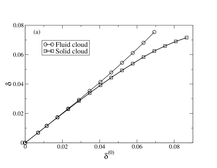
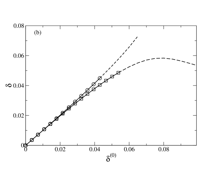
Figure 7: Polydispersities $\delta$ of shadow phases against the polydispersity of the parent, $\delta^{(0)}$, for (a) simulations of soft spheres, (b) MFE calculations for hard spheres.

The narrowing of the size distribution in the shadow solids can be quantified more precisely by plotting the polydispersity $\delta$ of the shadow solids against the polydispersity of the parent, which we here call $\delta^{(0)}$ for clarity. Fig. 7 shows that indeed the shadow solid has a lower polydispersity than the parent, an effect that gets more pronounced as $\delta^{(0)}$ increases. In the MFE calculations, where we can reach higher parent polydispersities, the solid shadow polydispersity in fact starts to decrease, a point already observed in Fig. 2. Conversely, the accumulation of the smallest and largest particles in the shadow liquid causes this phase to have a larger polydispersity than the parent.

VI Conclusions

In summary we have emphasised the necessity of fully catering for fractionation effects when performing theoretical and computational studies of phase equilibria in polydisperse systems. Failure to do so can – we believe – lead to qualitatively incorrect determinations of phase behaviour. In the context of simulation studies we have set out in detail the reasons why unconstrained density ensembles such as the $(\mu(\sigma),V,T)$ ensemble or the SGCE are superior to standard ($N,V,E$), ($N,V,T$) or ($N,p,T)$ ensembles with regard to their treatment of fractionation. The benefits of unconstrained ensembles were illustrated via an accurate determination of the polydispersity dependence of the freezing properties of size-disperse soft spheres. Our results, which are in good qualitative accord with moment free energy method calculations for hard spheres, show considerable fractionation of the incipient shadow phase that coexists with the parent when the coexistence region is entered from the fluid or solid side. Moreover, we find no evidence of the strong narrowing of the coexistence region with increasing polydispersity that is predicted by some theories Phan et al. (1998); Bartlett and Warren (1999) and simulations Phan et al. (1998); Huang and Xu (2004); Nogawa et al. (2010, ) that do not account fully for fractionation. Although our study considered only one particular form of the parent distribution (a top hat), previous MFE studies of other parent forms (triangular and Schulz distributions) find qualitatively similar behaviour Fasolo and Sollich (2004). We thus believe our findings for the nature of the freezing transition to be general.