From a single- to a double-well Penning trap

Abstract

The new generation of planar Penning traps promises to be a flexible and versatile tool for quantum information studies. Here, we propose a fully controllable and reversible way to change the typical trapping harmonic potential into a double-well potential, in the axial direction. In this configuration a trapped particle can perform coherent oscillations between the two wells. The tunneling rate, which depends on the barrier height and width, can be adjusted at will by varying the potential difference applied to the trap electrodes. Most notably, tunneling rates in the range of kHz are achievable even with a trap size of the order of 100 $\mu$m.

The challenging goal of using single electrons in Penning traps for quantum information marzoli ; ciaramicoli1 ; ciaramicoli6 ; ciaramicoli8 ; pedersen ; lamata has motivated intense research towards a completely new generation of devices. The so-called planar Penning traps stahl are specifically designed to meet the demands of quantum computation, thus allowing for scalability as well as improved addressability of the trapped particles. Moreover, new pixel microstructures promise to generate complex electric potentials, suitable both for particle transport and trapping in racetrack and artificial crystal configurations hellwig . The first planar Penning traps were operated in Mainz galve1 ; galve2 and in Ulm bushev1 both at room temperature and in a cryogenic environment. However, the elusive goal of a single trapped electron has not yet been achieved. The major obstacle is the anharmonicity in the axial potential, which prevents the detection of a single electron. To overcome this difficulty new theoretical studies goldman have carefully analyzed the geometry of planar Penning traps, with the aim of optimizing the harmonicity of the axial potential. The results are extremely encouraging and may lead to the first experimental demonstration of a single electron in a planar Penning trap.

Here we demonstrate the versatility of a planar Penning trap. In fact, it is able to produce a smooth variation of the trapping axial potential from a standard harmonic well into a double well. This result is achieved by applying suitable static voltages to the trap electrodes. The experimenter can control both the barrier height and width, simply by adjusting the potential difference between the electrodes. In particular, we have simulated the behavior of an optimized mirror-image planar Penning trap, which consists of two identical sets of electrodes facing each other. An electron, initially trapped in a single-well harmonic potential, can be adiabatically placed in a double-well potential. Depending on the energy of the axial motion, the particle wave function may spread over for several microns, through the barrier between the two wells. Therefore, the particle motional state could be prepared in a superposition of left and right, with the particle being, at the same time, in both wells. Hence, if a single electron trapped in a Penning trap forms a so-called geonium atom brown , the electron in the double-well potential can mimic a giant molecule along the lines of Ref. lesanovsky .

Moreover, this setup opens new perspectives for quantum information studies with a single trapped particle. Indeed, the position of the electron in the double-well potential may serve as a further qubit, encoding the $|0\rangle$ ($|1\rangle$) logical state in the left (right) well. Finally, the observation of a single particle, which performs Rabi oscillations between the two wells, could find application in interferometric schemes and precision sensing, as proposed for trapped ions in double-well potentials retzker .

A typical example of double-well potential is provided by the polynomial function

$$U(z)=az^{4}-bz^{2}$$ (1)

with $a$, $b>0$. In this case the distance between the two minima is $L=2\sqrt{b/(2a)}$, whereas the barrier height is $E_{b}=b^{2}/(4a)$.

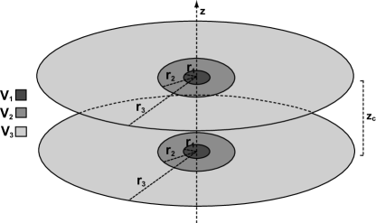
Figure 1: Schematic drawing of a mirror-image planar trap. Each electrode plane consists of a round central electrode with radius $r_{1}$ and two concentric ring electrodes with outer radii $r_{2}$ and $r_{3}$. The distance between the electrode planes is $z_{c}$.

We propose to realize such a double-well potential by means of a mirror-image planar Penning trap goldman . This device consists of a spatially uniform magnetic field, directed along the $z$ axis (axial direction), superimposed to an electrostatic field produced by two planar electrode structures, identically biased and facing each other. Each planar electrode arrangement is orthogonal to the $z$ axis and consists of a circular electrode of radius $r_{1}$ surrounded by two concentric rings with outer radii $r_{2}$ and $r_{3}$ (see Fig. 1). The two planar electrode sets are separated by a distance $z_{c}$. The $n$th electrode in each plane is held at the potential $V_{n}$. We assume that the radius of the second ring electrode $r_{3}$ is much larger than $r_{1}$, $r_{2}$ and than the distance $z_{c}$ between the two electrode sets. The trapping potential, along the $z$ axis, can be analytically calculated in the limit $r_{3}\rightarrow\infty$. To this end, we set the origin of the $z$ axis on the surface of the lower electrode plane and introduce the dimensionless parameters $\tilde{z}=z/r_{1}$, $\tilde{z}_{c}=z_{c}/r_{1}$ and $\tilde{r}_{i}=r_{i}/r_{1}$ with $i=1,2$. Hence, the electrostatic potential can be written as goldman

$$V(\tilde{z}) = (V_{2}-V_{1})[\phi_{1}(\tilde{z})+\phi_{1}(\tilde{z}_{c}-\tilde{z})]$$ (2)

$$+ (V_{3}-V_{2})[\phi_{2}(\tilde{z})+\phi_{2}(\tilde{z}_{c}-\tilde{z})]+V_{3},$$

where

$$\phi_{i}(\tilde{z})=\tilde{r}_{i}\int_{0}^{\infty}dk\,\frac{\sinh[k(\tilde{z}-\tilde{z}_{c})]}{\sinh(k\tilde{z}_{c})}\,J_{1}(k\tilde{r}_{i}),$$ (3)

with $J_{1}(z)$ being the Bessel function of the first kind.

Initially, we assume that the outermost ring electrode is grounded. With an appropriate choice of the voltages $V_{1}$ and $V_{2}$, the electrostatic potential takes on a parabolic shape with the minimum at a distance $z_{c}/2$ from the electrode surface goldman . Now we can smoothly pass from a single harmonic trap to a double-well one, by varying the potential $V_{3}$, applied to the second ring electrode (see Fig. 2). The distance between the two wells and the height of the energy barrier are controlled simply by adjusting the potential $V_{3}$.

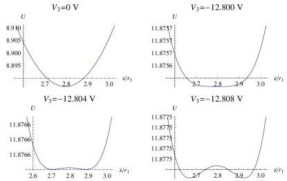
Figure 2: Plots showing the axial potential energy (in eV) of an electron near the center of a mirror-image planar Penning trap. We choose $\tilde{r}_{2}=4.45$, $\tilde{z}_{c}=5.6$, $V_{1}=-12.8$ V, and $V_{2}=-11.4$ V as in Ref. goldman . For each plot we specify the value of the potential $V_{3}$ applied to the second ring electrode.

The transition from a single- to a double-well trap can be better described by expanding the electrostatic potential, Eq. (2), in a power series near the trap center at $\tilde{z}=\tilde{z}_{c}/2$. As a consequence, the potential energy of an electron of charge $e$ takes on the form of Eq. (1) with

$$a = |e|[(V_{2}-V_{1})a_{1}+(V_{3}-V_{2})a_{2}],$$ (4)

$$b = |e|[(V_{2}-V_{1})b_{1}+(V_{3}-V_{2})b_{2}],$$ (5)

where

$$a_{i} = \frac{\tilde{r}_{i}}{24}\int_{0}^{\infty}dk\,k^{4}\frac{J_{1}(k\tilde{r}_{i})}{\cosh(k\tilde{z}_{c}/2)},$$ (6)

$$b_{i} = \frac{\tilde{r}_{i}}{2}\int_{0}^{\infty}dk\,k^{2}\frac{J_{1}(k\tilde{r}_{i})}{\cosh(k\tilde{z}_{c}/2)},\quad\mbox{with $i=1,2$}.$$ (7)

The transition from a single to a double well occurs when the parameter $b$ changes from negative to positive. This happens for $b=0$ when

$$V_{3}=[V_{2}(b_{2}-b_{1})+V_{1}b_{1}]/b_{2}.$$ (8)

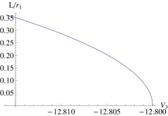
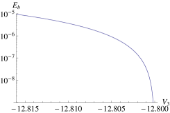
Figure 3: Top: plot of the well distance $L$, normalized to the the radius of the central disk electrode $r_{1}$, as a function of the potential $V_{3}$ (in volts) applied to the second ring electrode. Bottom: plot of the energy barrier (in eV) as a function of the potential $V_{3}$ (in volts). The values of $\tilde{r}_{2}$, $\tilde{z}_{c}$, $V_{1}$ and $V_{2}$ are the same as in Fig. 2.

Since the well distance $L$ and the energy barrier height $E_{b}$ are related to the coefficients $a$ and $b$, we can calculate how these parameters vary with the voltage $V_{3}$ (see Fig. 3). The distance between the two minima depends also on the radius of the central electrode, whereas the energy barrier height does not depend on the actual trap size. For example, in an optimized mirror-image planar trap with $r_{1}=100$ $\mu$m, $\tilde{r}_{2}=4.45$, $\tilde{z}_{c}=5.6$, $V_{1}=-12.8$ V, $V_{2}=-11.4$ V and $V_{3}=-12.8013$ V we obtain a double-well potential with minima separated by a distance $L=10$ $\mu$m and barrier height $E_{b}=6\times 10^{-8}$ eV. In this case, the coefficients $b_{1}$ and $b_{2}$ are approximately equal and, therefore, according to Eq. (8) the transition from a single- to a double-well trap occurs for $V_{3}\simeq V_{1}$.

The oscillation frequency of an electron, in each well, can be estimated by expanding its potential energy, Eq. (1), in a power series near the minima at $z=\pm\sqrt{b/2a}$. Also the angular oscillation frequency depends on the width and the height of the energy barrier

$$\omega_{z}=\frac{4}{L}\sqrt{\frac{2E_{b}}{m}},$$ (9)

with $m$ being the electron mass. The behavior of the axial frequency $\omega_{z}/2\pi$ is plotted in Fig. 4 as a function of the barrier height, for different values of the well distance. In the case of a double well with $L=10$ $\mu$m and barrier height $E_{b}=6\times 10^{-8}$ eV, we expect an axial frequency $\omega_{z}/2\pi=10$ MHz.

Figure 4: Plot of the electron axial frequency $\omega_{z}/2\pi$ (in Hz) as a function of the barrier height (in eV) for different choices of the well distance $L$. For each value of $L$, there is a minimum value of the barrier height below which the electron motion is not confined to a single well.

Let us give a more in-depth analysis of the dynamics of a single electron in a double-well Penning trap. As in usual Penning traps, the radial motion (in the $xy$ plane) and the spin motion are practically decoupled from the axial motion. Hence, in the following we disregard the radial and spin degrees of freedom and consider only the electron motion along the $z$ axis. The dynamics of this one-dimensional system is governed by the following Schrödinger equation

$$i\hbar\frac{\partial\Psi(z,t)}{\partial t}=-\frac{\hbar^{2}}{2m}\frac{\partial^{2}\Psi(z,t)}{\partial z^{2}}+eV(z)\Psi,$$ (10)

where $\Psi(z,t)$ is the axial wave function of an electron in the electrostatic potential $V(z)$, produced by the trap electrodes.

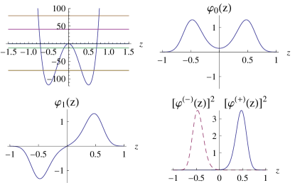
Figure 5: The panels show: the double well potential energy, Eq. (1), with the first few energy levels, the probability amplitude of the first eigenstate $\varphi_{0}$, the probability amplitude of the second eigenstate $\varphi_{1}$, and the probability density of the localized states $\varphi^{(\pm)}$. The two lowest energy eigenvalues appear indistinguishable in the plot. Energies and lengths are expressed, respectively, in units of $\hbar^{2}/2mL^{2}$ and $L$.

To determine the evolution of $\Psi(z,t)$ we have to find eigenvalues and eigenstates of the system Hamiltonian by solving the time independent Schrödinger equation

$$-\frac{\hbar^{2}}{2m_{e}}\frac{d^{2}\varphi(z)}{dz^{2}}+eV(z)\varphi(z)=E\varphi(z).$$ (11)

Let us indicate with $\{\varphi_{0},\varphi_{1},\ldots\}$ the set of energy eigenstates and with $\{E_{0},E_{1},\ldots\}$ the corresponding eigenvalues solutions of Eq. (11). As a consequence of the double well shape, the energy eigenvalues appear as a series of pairs of nearby values. We focus on the two eigenstates corresponding to the lowest energy eigenvalues, that we suppose being smaller than the height of the barrier between the two wells. The higher the barrier the smaller the energy difference between these levels. In the limit of an infinitely high barrier, these two energy eigenstates tend to become degenerate. Because of the symmetry of the potential energy, eigenstates have a definite parity: the eigenstate $\varphi_{0}$ is even and has zero nodes, whereas the eigenstate $\varphi_{1}$ is odd and has one node (see Fig. 5).

Given the pair of eigenstates $\varphi_{0}$ and $\varphi_{1}$ we can construct two orthogonal states $\varphi^{(+)}$ and $\varphi^{(-)}$ defined as

$$\varphi^{(\pm)}=\frac{1}{\sqrt{2}}(\varphi_{0}\pm\varphi_{1}).$$ (12)

An electron prepared in the state $\varphi^{(+)}$ [$\varphi^{(-)}$] is localized in the right (left) well, as displayed in Fig. 5. However, since the states $\varphi^{(\pm)}$ are not stationary, the particle tunnels through the barrier, oscillating back and forth between the two wells. For a particle initially localized in the right well, the state of the system at a later time $t$ is described by

$$\Psi(z,t)=\frac{1}{\sqrt{2}}\left[\varphi_{0}(z)e^{-i\frac{E_{0}t}{\hbar}}+\varphi_{1}(z)e^{-i\frac{E_{1}t}{\hbar}}\right].$$ (13)

Hence, the probability density to find the electron in the $z$ direction is

$$|\Psi(z,t)|^{2}=\frac{1}{2}[\varphi_{0}^{2}(z)+\varphi_{1}^{2}(z)+2\varphi_{0}(z)\varphi_{1}(z)\cos(\omega_{1,0}t)],$$ (14)

where $\omega_{1,0}\equiv(E_{1}-E_{0})/\hbar$. In terms of the states $\varphi^{(\pm)}$ we can recast Eq. (14) as

$$|\Psi(z,t)|^{2}=\left[\varphi^{(+)}\right]^{2}\cos^{2}\left(\frac{\omega_{1,0}t}{2}\right)+\left[\varphi^{(-)}\right]^{2}\sin^{2}\left(\frac{\omega_{1,0}t}{2}\right).$$ (15)

From Eq. (15) we clearly see that the electron oscillates between the two wells at the tunneling frequency $\omega_{1,0}/2\pi$.

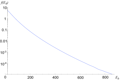
Figure 6: Plot of the numerically calculated dimensionless quantity $f(E_{b})$ as a function of the barrier height $E_{b}$ measured in units of $\hbar^{2}/2mL^{2}$.

Let us consider a double-well potential energy described by the polynomial function of Eq. (1). We have numerically calculated the energy eigenstates and eigenvalues for different values of the energy barrier $E_{b}$ and of the distance $L$ between the two wells. From this numerical analysis, we have deduced the following relation

$$\frac{\omega_{1,0}}{2\pi}=\frac{f(E_{b})}{4\pi mL^{2}}=\frac{f(E_{b})}{L^{2}}\times 9.18\times 10^{-6}\,\mbox{Hz m}^{2},$$ (16)

which expresses the dependence of the tunneling frequency upon the double well parameters. The behavior of the dimensionless function $f$ is represented in Fig. 6. Given the barrier height $E_{b}$ and width $L$, one can calculate the corresponding tunneling frequency by means of Eq. (16).

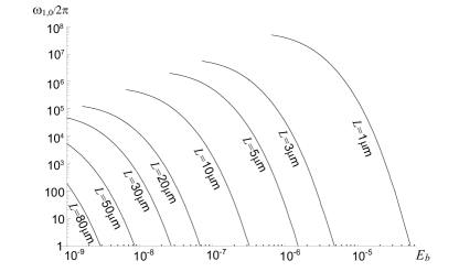
Figure 7: The tunneling frequency $\omega_{1,0}/2\pi$ (in Hz) as a function of the barrier height (in eV) for different values of the well distance. Notice that, for any given well distance, there is a minimum value of the energy barrier, below which the wells cannot longer accomodate the two lowest energy eigenvalues. In this case we cannot define a tunneling frequency $\omega_{1,0}$.

In Fig. 7 it is plotted the tunneling frequency $\omega_{1,0}/2\pi$ as a function of the double well barrier height, for different choices of the well distance $L$.

In particular, for a double well with a distance betweeen the minima $L=10$ $\mu$m and a barrier height $E_{b}=6\times 10^{-8}$ eV the tunneling frequency for an electron is $\omega_{1,0}/2\pi=50$ kHz. This value is achievable with an optimized mirror-image planar Penning trap of the kind proposed by Ref. goldman , whose central disc electrode has a radius of 100 $\mu$m. Also the required control and stability of the applied voltages is within the reach of present technology. Hence, it seems feasible to employ the same physical device to produce both a perfectly harmonic axial potential and a double-well one. This possibility opens new perspectives and applications for a single trapped electron in a planar Penning trap. The observation of the electron oscillations between the two wells could provide insight into the coherence properties of the system and measure its sensitivity to technical imperfections and environmental noise.

References

- (1) For a review see: I. Marzoli et al., J. Phys. B: At. Mol. Opt. Phys. 42, 154010 (2009) and references therein.
- (2) G. Ciaramicoli, I. Marzoli, and P. Tombesi, Phys. Rev. Lett. 91, 017901 (2003).
- (3) G. Ciaramicoli, I. Marzoli, and P. Tombesi, Phys. Rev. A 75, 032348 (2007).
- (4) G. Ciaramicoli, I. Marzoli, and P. Tombesi, Phys. Rev. A 78, 012338 (2008).
- (5) L. H. Pedersen and C. Rangan, Quantum Information Processing 7, 33 (2008).
- (6) L. Lamata, D. Porras, J. I. Cirac, J. Goldman, and G. Gabrielse, Phys. Rev. A 81, 022301 (2010).
- (7) S. Stahl, F. Galve, J. Alonso, S. Djekic, W. Quint, T. Valenzuela, J. Verdú, M. Vogel, and G. Werth, Eur. Phys. J. D 32, 139 (2005).
- (8) M. Hellwig, A. Bautista-Salvador, K. Singer, G. Werth, and F. Schmidt-Kaler, New J. Phys. 12, 065019 (2010).
- (9) F. Galve, P. Fernandez, and G. Werth, Eur. Phys. J. D 40, 201 (2006).
- (10) F. Galve and G. Werth, Hyperfine Interact. 174, 41 (2007).
- (11) P. Bushev, S. Stahl, R. Natali, G. Marx, E. Stachowska, G. Werth, M. Hellwig, and F. Schmidt-Kaler, Eur. Phys. J. D 50, 97 (2008).
- (12) J. Goldman and G. Gabrielse, Phys. Rev. A 81, 052335 (2010).
- (13) L. S. Brown and G. Gabrielse, Rev. Mod. Phys. 58, 233 (1986).
- (14) I. Lesanovsky, M. Müller, and P. Zoller, Phys. Rev. A 79, 010701(R) (2009).
- (15) A. Retzker, R. C. Thompson, D. M. Segal, and M. B. Plenio, Phys. Rev. Lett. 101, 260504 (2008).