On the Performance of Spectrum Sensing Algorithms using Multiple Antennas

Abstract

In recent years, some spectrum sensing algorithms using multiple antennas, such as the eigenvalue based detection (EBD), have attracted a lot of attention. In this paper, we are interested in deriving the asymptotic distributions of the test statistics of the EBD algorithms. Two EBD algorithms using sample covariance matrices are considered: maximum eigenvalue detection (MED) and condition number detection (CND). The earlier studies usually assume that the number of antennas $(K)$ and the number of samples $(N)$ are both large, thus random matrix theory (RMT) can be used to derive the asymptotic distributions of the maximum and minimum eigenvalues of the sample covariance matrices. While assuming the number of antennas being large simplifies the derivations, in practice, the number of antennas equipped at a single secondary user is usually small, say $2$ or $3$, and once designed, this antenna number is fixed. Thus in this paper, our objective is to derive the asymptotic distributions of the eigenvalues and condition numbers of the sample covariance matrices for any fixed $K$ but large $N$, from which the probability of detection and probability of false alarm can be obtained. The proposed methodology can also be used to analyze the performance of other EBD algorithms. Finally, computer simulations are presented to validate the accuracy of the derived results.

I Introduction

Spectrum sensing is one of the key elements in opportunistic spectrum access design [1], [2]. In literature, there are a few main categories of practical spectrum sensing schemes for OSA including: energy detection, cyclostationarity based detection, and eigenvalue-based detection (EBD); see, e.g. [3] and references therein. Energy detection is simple for implementation, however, it requires accurate noise power information, and a small error in that estimation may cause SNR wall and high probability of false alarm [4]. For cyclostationarity based detection, the cyclic frequency of PU’s signal needs to be acquired a priori. On the other hand, EBD [5], first proposed and submitted to IEEE 802.22 working group [6], performs signal detection by estimating the signal and noise powers simultaneously, thus it does not require the cyclic knowledge of the PU and is robust to noise power uncertainty.

In general, two steps are needed to complete a sensing design: (1) to design the test statistics; and (2) to derive the probability density function (PDF) of the test statistics. For spectrum sensing with multiple antennas, the test statistics can be designed based on the standard principles such as generalized likelihood ratio testing (GLRT) [7], or other considerations [5], [8], [9], [10]. Surprisingly these studies all give the test statistics using the eigenvalues of the sample covariance matrix. It is thus important to derive the PDF of the eigenvalues so that the sensing performance can be quantified.

For EBD schemes, the PDF of the test statistics is usually derived using random matrix theory (RMT); see, e.g., [5], [8], [9], [10]. In fact, the maximum and minimum eigenvalues of the sample covariance matrix have simple explicit expressions when both antenna number ($K$) and ample size ($N$) are large [11, 12]. It is reasonable to assume that $N$ is large especially when the secondary user is required to sense a weak primary signal, in practice, however, the number of antennas equipped at a single secondary user is usually small, say $2$ or $3$. Thus the results obtained under the assumption that both $K$ and $N$ are large may not be accurate for practical multi-antenna cognitive radios. In this paper, our objective is to derive the asymptotic distributions of the eigenvalues of the sample covariance matrices for arbitrary $K$ but large $N$. The asymptotic results obtained form the basis for quantifying the PDF of the test statistics for EBD algorithms.

It is noticed that there are studies on the exact distribution of the condition number of sample covariance matrices for arbitrary $K$ and $N$ [13], the formulas derived however are complex and cannot be conveniently used to analyze the sensing performance. Furthermore, there are no results published for the case when the primary signals exist.

The rest of the paper is organized as follows. Section II presents the system model for spectrum sensing using multiple antennas. Two EBD algorithms are reviewed in Section III, including maximum eigenvalue detection (MED) and condition number detection (CND) algorithms. In Section IV, we derive the asymptotic distributions of the test statistics of the two EBD algorithms for the scenario when the primary users are inactive. In Section V, the results are derived for the scenario when there are active primary users in the sensed band. Performance evaluations are given in Section VI, and finally, conclusions are drawn in Section VII.

The following notations are used in this paper. Matrices and vectors are typefaced using bold uppercase and lowercase letters, respectively. Conjugate transpose of matrix ${\bf A}$ is denoted as ${\bf A}^{H}$. $\|{\bf a}\|$ stands for the norm of vector ${\bf a}$. $\mathbb{E}[\cdot]$ denotes expectation operation; $\stackrel{{\scriptstyle D}}{{\longrightarrow}}$, $\stackrel{{\scriptstyle a.s.}}{{\longrightarrow}}$ and $\stackrel{{\scriptstyle\Delta}}{{=}}$ stand for “convergence in distribution”, “almost surely convergence”; and “defined as”, respectively.

II System Model

Suppose the SU is equipped with $K$ antennas, which are all used to sense a radio spectrum for collecting $N$ samples each. One of the following two scenarios happens.

Scenario 1 ($\mathcal{S}_{1}$): There are $t~{}(t\geq 1)$ active PU transmissions in the sensed band, and the sampled outputs, ${\bf x}(n)$, $n=0,\cdots,N-1$, can be represented as

$${\bf x}(n)={\bf H}{\bf s}(n)+{\bf u}(n),$$ (1)

where ${\bf u}(n)$ is the $(K\times 1)$ noise vector, ${\bf s}(n)$ is the $(t\times 1)$ signal vector containing the transmitted signals from the active PUs, and ${\bf H}=[{\bf h}_{1},\cdots,{\bf h}_{t}]$ is the $(K\times t)$ channel matrix from the active PUs to the SU.

Scenario 0 ($\mathcal{S}_{0}$): There are no active PUs in the sensed band, thus the sampled outputs collected at SU are given by

$${\bf x}(n)={\bf u}(n).$$ (2)

We make the following assumptions for the above models:

• The noises ${\bf u}(n)$ are independent and identically distributed (iid) both spatially and temporally. Each element follows Gaussian distribution with mean zero and variance $\sigma_{u}^{2}$.

• For each $n$, the elements of ${\bf s}(n)$ are iid, and follow Gaussian distribution with mean zero and variance $\sigma_{s}^{2}$. Thus the covariance matrix of ${\bf s}(n)$ is ${\bf R}_{s}\stackrel{{\scriptstyle\Delta}}{{=}}\mathbb{E}[{\bf s}(n){\bf s}^{H}(n)]=\sigma_{s}^{2}{\bf I}$.

• ${\bf s}(n)$ are ${\bf u}(n)$ are independent of each other.

• The eigenvalues of ${\bf H}{\bf H}^{H}$ are not all identical.

Two cases of Gaussian distribution are considered: (1) Real-valued case: we denote ${\bf u}(n)\sim\mathcal{N}({\bf 0},\sigma_{u}^{2}{\bf I})$ and ${\bf s}(n)\sim\mathcal{N}({\bf 0},\sigma_{s}^{2}{\bf I})$; (2) Complex-valued case: We denote ${\bf u}(n)\sim\mathcal{CN}({\bf 0},\sigma_{u}^{2}{\bf I})$ and ${\bf s}(n)\sim\mathcal{CN}({\bf 0},\sigma_{s}^{2}{\bf I})$;

When there are active PUs, we define the average received signal-to-noise ratio (SNR) of PUs’ signals measured at SU as : $\mbox{SNR}=\frac{\sum_{\ell=1}^{t}\|{\bf h}_{\ell}\|^{2}\sigma_{s}^{2}}{K\sigma_{u}^{2}}$. Given the received samples, ${\bf X}=[{\bf x}(0),{\bf x}(1),\cdots,{\bf x}(N-1)]$, the objective of spectrum sensing design is to choose one of the two hypothesis: $\mathcal{H}_{0}$: there are no active primary users in the sensed band, and $\mathcal{H}_{1}$: there exist active primary users. For that, we need to design the test static, $T({\bf X})$, and a threshold $\epsilon$, and infer $\mathcal{H}_{1}$ if $T({\bf X})>\epsilon$, and infer $\mathcal{H}_{0}$ if $T({\bf X})\leq\epsilon$.

III Eigenvalue based Detections

Let us define the sample covariance matrix and covariance matrix of the measurements ${\bf x}(n)$ of the sensed band as

$$\hat{\bf R}_{x} \stackrel{{\scriptstyle\Delta}}{{=}} \frac{1}{N}{\bf X}{\bf X}^{H}=\frac{1}{N}\sum_{n=0}^{N-1}{\bf x}(n){\bf x}^{H}(n),$$ (3)

$${\bf R}_{x} \stackrel{{\scriptstyle\Delta}}{{=}} \mathbb{E}[{\bf x}(n){\bf x}^{H}(n)],$$ (4)

respectively. For a fixed $K$, under Scenario $\mathcal{S}_{0}$ and when $N\to\infty$, we have

$$\hat{\bf R}_{x}\to{\bf R}_{x}=\sigma_{u}^{2}{\bf I},$$ (5)

which means that all the eigenvalues of the covariance matrix are equal to $\sigma_{u}^{2}$. However, under $\mathcal{S}_{1}$ and when $N\to\infty$, $\hat{\bf R}_{x}$ approaches

$${\bf R}_{x}=\sigma_{s}^{2}{\bf H}{\bf H}^{H}+\sigma_{u}^{2}{\bf I}.$$ (6)

Based on assumption (iv), the eigenvalues of (6) can be ordered as $\rho_{1}\geq\rho_{2}\geq\cdots\geq\rho_{K}\geq\sigma_{u}^{2}$.

Denote the ordered eigenvalues of the sample covariance matrix $\hat{\bf R}_{x}$ as $\hat{\lambda}_{1}\geq\hat{\lambda}_{2}\geq\cdots\geq\hat{\lambda}_{K}$. We consider the following two EBD algorithms.

• Maximum Eigenvalue Detection (MED): For MED, the test static is chosen as [8]:

  $$T^{(m)}({\bf X})=\frac{\hat{\lambda}_{1}}{\sigma_{u}^{2}}.$$ (7)

• Condition Number Detection (CND): The CND chooses the following test statistic [5]:

  $$T^{(c)}({\bf X})=\frac{\hat{\lambda}_{1}}{\hat{\lambda}_{K}}.$$ (8)

An essential task to complete the sensing design is to determine the test threshold, which affects both probability of detection and probability of false alarm. To do so, it is important to derive the PDF of the test statistics.

For arbitrary $(K,N)$ pair, the closed-form expressions of the PDF of the test statics are in general complex [13]. In practice, the primary users need to be detectable in low SNR environment. For example, in IEEE 802.22, the TV signal needs to be detected at $-20$dB SNR with $90\%$ target probability of detection and $10\%$ target probability of false alarm. To achieve that, the number of samples, $N$, required for spectrum sensing is usually very large. In the paper, we thus turn our attention to derive the PDFs of the test statistics for any fixed $K$, but large $N$. The asymptotic distributions (when $N\to\infty$) of the test statics of the EBD algorithms will be derived for $\mathcal{S}_{0}$ and $\mathcal{S}_{1}$ scenarios, respectively.

IV Asymptotic Distributions of the Test Statistics under Scenario $\mathcal{S}_{0}$

Let $\lambda_{i}=\frac{\hat{\lambda}_{i}}{\sigma_{u}^{2}}$ for $i=1,\cdots,K$, and denote ${\bf A}=\mbox{diag}\left\{\lambda_{1},\lambda_{2},\cdots,\lambda_{K}\right\}$. Define $\beta_{i}=\sqrt{N}(\lambda_{i}-1)$ for $i=1,\cdots,K$, and ${\bf B}=\mbox{diag}\left\{\beta_{1},\beta_{2},\cdots,\beta_{K}\right\}$. Note that $\beta_{1}\geq\beta_{2}\geq\cdots\geq\beta_{K}$.

Under $\mathcal{S}_{0}$, by Theorem 1 and (2.12) in [14], we have the following proposition.

Proposition 1

For real-valued case, when $N\to\infty$, the limiting distribution of ${\bf B}$, $g_{K}(\beta_{1},\beta_{2},\cdots,\beta_{K})$, is given by

$$g_{K}(\beta_{1},\cdots,\beta_{K})$$ (9)

$$= C_{1}(K)\exp\left(-\frac{1}{4}\sum\limits_{i=1}^{K}\beta_{i}^{2}\right)\prod_{1\leq i<j\leq K}(\beta_{i}-\beta_{j}),$$

where

$$C_{1}(K)=\frac{1}{2^{K(K+3)/4}\prod_{i=1}^{K}\Gamma[\frac{1}{2}(K+1-i)]}.$$ (10)

Here $\Gamma(z)=\int_{0}^{\infty}t^{z-1}e^{-t}dt$ is the Gamma function.

For real-valued case, and when $K=1$, we have $\beta_{1}\sim\mathcal{N}(0,2)$, i.e., $g_{1}(\beta_{1})=\frac{1}{2\sqrt{\pi}}e^{-\frac{\beta_{1}^{2}}{4}}$. When $K=2$, we have

$$g_{2}(\beta_{1},\beta_{2})=\frac{1}{2^{5/2}\sqrt{\pi}}(\beta_{1}-\beta_{2})e^{-\frac{\beta_{1}^{2}+\beta_{2}^{2}}{4}},\quad\beta_{1}\geq\beta_{2}.$$ (11)

For complex-valued case, by Lindberg’s central limit theorem [15], $\sqrt{N}(\frac{\hat{\bf R}_{x}}{\sigma_{u}^{2}}-{\bf I})$ converges to a Hermitian matrix with elements above diagonal being complex Gaussian distribution, a so-called Gaussian unitary matrix. Thus, according to the joint density of the eigenvalues of a Gaussian unitary matrix, similar to Theorem 1 in [14] we have the following:

Proposition 2

For complex-valued case, when $N\to\infty$, the limiting distributions of ${\bf B}$, $g_{K}(\beta_{1},\beta_{2},\cdots,\beta_{K})$, is given by

$$g_{K}(\beta_{1},\cdots,\beta_{K})$$ (12)

$$= C_{2}(K)\exp\left(-\frac{1}{2}\sum\limits_{i=1}^{K}\beta_{i}^{2}\right)\prod_{1\leq i<j\leq K}(\beta_{i}-\beta_{j})^{2},$$

where

$$C_{2}(K)=K!(2\pi)^{-K/2}\prod_{j=1}^{K}\frac{1}{\Gamma(1+j)}.$$ (13)

For complex-valued case, when $K=1$, we have $g(\beta_{1})=\frac{1}{\sqrt{2\pi}}e^{-\frac{\beta_{1}^{2}}{2}}$, i.e., $\beta_{1}\sim\mathcal{N}(0,1)$. When $K=2$, we have

$$g_{2}(\beta_{1},\beta_{2})=\frac{1}{2\pi}(\beta_{1}-\beta_{2})^{2}e^{-\frac{\beta_{1}^{2}+\beta_{2}^{2}}{2}},\quad\beta_{1}\geq\beta_{2}.$$ (14)

For a given $K$, the limiting distribution, $\bar{g}_{K,i}(x)$, of $\beta_{i},i=1,\cdots,K$, can be calculated from (9) or (12).

IV-A MED

For MED, $T^{(m)}({\bf X})=\frac{\hat{\lambda}_{1}}{\sigma_{u}^{2}}=\lambda_{1}$, thus $\sqrt{N}(T^{(m)}({\bf X})-1)=\beta_{1}$. We have the following:

Theorem 1

Under $\mathcal{S}_{0}$, for a fixed $K$ and when $N\to\infty$,

$$\sqrt{N}\left(T^{(m)}({\bf X})-1\right)\stackrel{{\scriptstyle D}}{{\longrightarrow}}m_{K}^{(0)},$$ (15)

whose distribution, $f_{K}^{(m)}(x)$, is the same as the limiting distribution of $\beta_{1}$, $\bar{g}_{K,1}(x)$.

IV-B CND

For CND, $T^{(c)}({\bf X})=\frac{\hat{\lambda}_{1}}{\hat{\lambda}_{K}}=\frac{\lambda_{1}}{\lambda_{K}}$. The following theorem states the limiting distribution of the condition number of the sample covariance matrix.

Theorem 2

Under $\mathcal{S}_{0}$, for a fixed $K$ and when $N\to\infty$,

$$\sqrt{N}\left(T^{(c)}({\bf X})-1\right)\stackrel{{\scriptstyle D}}{{\longrightarrow}}z_{K}^{(0)},$$ (16)

whose PDF and cumulative density function (CDF) are given by

$$f_{K}^{(c)}(x) = \int^{\infty}_{-\infty}\tilde{g}_{K}(\beta_{K}+x,\beta_{K})d\beta_{K},$$ (17)

$$F_{K}^{(c)}(x) = \int^{\infty}_{-\infty}\int_{\beta_{K}}^{\beta_{K}+x}\tilde{g}_{K}(\beta_{1},\beta_{K})d\beta_{1}d\beta_{K},$$ (18)

respectively, where $\tilde{g}_{K}(\beta_{1},\beta_{K})$ is the joint distribution of $\beta_{1}$ and $\beta_{K}$.

Proof:

See [16]. ∎

Next, we derive the closed-form expressions of the limiting distributions of the condition number of the sample covariance matrix for $K=2$ case.

Lemma 1

Consider Scenario $\mathcal{S}_{0}$. For $K=2$ and $N\to\infty$,

$$\sqrt{N}\left(T^{(c)}({\bf X})-1\right)\stackrel{{\scriptstyle D}}{{\longrightarrow}}z_{2}^{(0)},$$ (19)

whose PDF is

$$f_{2}^{(c)}(x)=\frac{1}{4}x\exp(-x^{2}/8),\qquad x\geq 0,$$ (20)

for real-valued case, and

$$f_{2}^{(c)}(x)=\frac{1}{2\sqrt{\pi}}x^{2}e^{-x^{2}/4},\qquad x\geq 0.$$ (21)

for complex-valued case.

IV-C Threshold Determination

From the above two subsections, it is seen that for a given $K$ and when $N\to\infty$, the regulated test statistics, $\sqrt{N}(T^{(i)}({\bf X})-1)$ converges to a random variable with PDF $f_{K}^{(i)}(x)$ and CDF $F_{K}^{(i)}(x)$, where $i=m$ for MED and $i=c$ for CND. Here, we look at how to set the decision threshold $\epsilon$ to achieve a target probability of false alarm, $\bar{P}_{f}$. Since

$$\bar{P}_{f} = \mbox{Prob}~{}\left(T^{(i)}({\bf X})>\epsilon|\mathcal{S}_{0}\right)$$ (22)

$$= \mbox{Prob}~{}\left(\sqrt{N}\left(T^{(i)}({\bf X})-1\right)>\sqrt{N}(\epsilon-1)|\mathcal{S}_{0}\right)$$

$$= 1-\int_{0}^{\sqrt{N}(\epsilon-1)}f_{K}^{(i)}(t)dt$$

$$= 1-F_{K}^{(i)}(\sqrt{N}(\epsilon-1)).$$

Thus the decision threshold is determined by

$$\epsilon=1+\frac{1}{\sqrt{N}}[F_{K}^{(i)}]^{-1}(1-\bar{P}_{f}),$$ (23)

where $x=[F_{K}^{(i)}]^{-1}(y)$ denotes the inverse function of $y=F_{K}^{(i)}(x)$.

V Asymptotic Distributions of the Test Statistics under Scenario $\mathcal{S}_{1}$

In this section, we derive the asymptotic distributions of the test statistics under $\mathcal{S}_{1}$. Consider the ordered eigenvalues of covariance matrix ${\bf R}_{x}$, $\rho_{1}\geq\rho_{2}\geq\cdots\geq\rho_{K}$, and the ordered eigenvalues of sample covariance matrix $\hat{{\bf R}}_{x}$, $\hat{\lambda}_{1}\geq\hat{\lambda}_{2}\geq\cdots\geq\hat{\lambda}_{K}$. With the same notation as in [14], let the multiplicities of the eigenvalues of ${\bf R}_{x}$ be $q_{1},q_{2},\cdots,q_{r}$. That is

$$\rho_{1}=\cdots=\rho_{q_{1}}=\mu_{1},$$

$$\rho_{q_{1}+1}=\cdots=\rho_{q_{1}+q_{2}-1}=\mu_{2},$$

$$\rho_{K-q_{r}+1}=\cdots=\rho_{K}=\mu_{r},$$

where

$$\mu_{1}>\mu_{2}>\cdots>\mu_{r}.$$

Moreover, let

$${\bf{\Gamma}}^{H}{\bf{R}}_{x}{\bf{\Gamma}}={\bf{\Delta}},$$

$${\bf E}^{H}{\bf{\Gamma}}^{H}\hat{\bf{R}}_{x}{\bf{\Gamma}}{\bf E}={\bf B},$$

where

$${\bf{\Delta}}=\mbox{diag}(\rho_{1},\rho_{2},\cdots,\rho_{K}),$$

$${\bf B}=\mbox{diag}(\hat{\lambda}_{1},\hat{\lambda}_{2},\cdots,\hat{\lambda}_{K}),$$

and $\bf{\Gamma}$ and ${\bf E}$ are corresponding eigenvector matrices. We then partition the matrices ${\bf{\Delta}}$ and ${\bf B}$ into block matrices as follows:

$$\bf{\Delta}=\begin{pmatrix}\mu_{1}{\bf I}&0&\cdots&0\\ 0&\mu_{2}{\bf I}&\cdots&0\\ \vdots&\vdots&\ &\vdots\\ 0&0&\cdots&\mu_{r}{\bf I}\end{pmatrix},$$ (24)

$${\bf B}=\begin{pmatrix}{\bf B}_{1}&0&\cdots&0\\ 0&{\bf B}_{2}&\cdots&0\\ \vdots&\vdots&\ &\vdots\\ 0&0&\cdots&{\bf B}_{r}\end{pmatrix}.$$ (25)

Note in both ${\bf{\Delta}}$ and ${\bf B}$, the $k$th diagonal sub-block is $q_{k}\times q_{k}$ matrix.

Following the proofs of Proposition 1 and Proposition 2, and Theorem 1 of [14], we have the following results.

Theorem 3

The limiting distribution of $\sqrt{N}\left(\frac{{\bf B}_{k}}{\mu_{k}}-{\bf I}\right)$ is given by (9) and (12) for real-valued case and complex-valued case, respectively, with the parameter $K$ being replaced by $q_{k}$. Furthermore, $\sqrt{N}\left(\frac{{\bf B}_{i}}{\mu_{i}}-{\bf I}\right)$ is asymptotically independent of $\sqrt{N}\left(\frac{{\bf B}_{j}}{\mu_{j}}-{\bf I}\right)$ for $i\neq j$.

Let $\gamma_{1}=\sqrt{N}(\frac{\hat{\lambda}_{1}}{\mu_{1}}-1)$ and $\gamma_{K}=\sqrt{N}(\frac{\hat{\lambda}_{K}}{\mu_{r}}-1)$. From Theorem 3, $\gamma_{1}$ and $\gamma_{K}$ are asymptotically independent, and the limiting distributions of $\gamma_{1}$ and $\gamma_{K}$ are $\bar{g}_{q_{1},1}(x)$ and $\bar{g}_{q_{r},q_{r}}(x)$, respectively, which are defined in Section IV.

V-A MED

For MED, $T^{(m)}({\bf X})=\frac{\hat{\lambda}_{1}}{\sigma_{u}^{2}}$, thus $\frac{\hat{\lambda}_{1}}{\mu_{1}}=\alpha^{(m)}T^{(m)}({\bf X})$ where $\alpha^{(m)}=\frac{\sigma_{u}^{2}}{\mu_{1}}$. We have the following theorem.

Theorem 4

Under $\mathcal{S}_{1}$, when $N\to\infty$,

$$\sqrt{N}\left(\alpha^{(m)}T^{(m)}({\bf X})-1\right)\stackrel{{\scriptstyle D}}{{\longrightarrow}}m_{K}^{(1)},$$ (26)

whose PDF is $\bar{g}_{q_{1},1}(x)$.

If there are no repeated maximum eigenvalues (i.e., $q_{1}=1$), $m_{K}^{(1)}\sim\mathcal{N}(0,2)$ for real-valued case, and $m_{K}^{(1)}\sim\mathcal{N}(0,1)$ for complex-valued case.

V-B CND

For CND, $T^{(c)}({\bf X})=\frac{\hat{\lambda}_{1}}{\hat{\lambda}_{K}}$. Since $\gamma_{1}$ and $\gamma_{K}$ are asymptotically independent, and when $N\to\infty$, $\frac{\hat{\lambda}_{1}}{\mu_{1}}\stackrel{{\scriptstyle a.s.}}{{\longrightarrow}}1$, $\frac{\hat{\lambda}_{K}}{\mu_{r}}\stackrel{{\scriptstyle a.s.}}{{\longrightarrow}}1$, similar to Theorem 2, we have the following theorem.

Theorem 5

Under $\mathcal{S}_{1}$, for a fixed $K$ and when $N\to\infty$,

$$\sqrt{N}\left(\alpha^{(c)}T^{(c)}({\bf X})-1\right)\stackrel{{\scriptstyle D}}{{\longrightarrow}}c_{K}^{(1)},$$ (27)

where $\alpha^{(c)}=\frac{\mu_{r}}{\mu_{1}}$, and the PDF of $c_{K}^{(1)}$ is given by

$$w_{K}^{(c)}(x) = \int^{\infty}_{-\infty}\bar{g}_{1,1}(x+y)\bar{g}_{q_{r},q_{r}}(y)dy.$$ (28)

Now let us look at the case when $q_{1}=q_{r}=1$. Since both $\gamma_{1}$ and $\gamma_{K}$ follow the same Gaussian distribution asymptotically, we can easily derive that $c_{K}^{(1)}\sim\mathcal{N}(0,4)$ for real-valued case, and $c_{K}^{(1)}\sim\mathcal{N}(0,2)$ for complex-valued case.

VI Computer Simulations

Computer simulations are presented in this section to validate the effectiveness of the results obtained in this paper. We choose $K=2$, and there is one primary signal under $\mathcal{S}_{1}$. $10000$ Monte Carlo runs are carried out in order to compute CDF of the test statistics.

VI-A Scenario $\mathcal{S}_{0}$

We first compare the CDFs of the regulated test statistics $\sqrt{N}(T^{(m)}({\bf X})-1)$ for MED derived using computer simulations, and theoretic analysis under fixed $K$ assumption of this paper and large $K$ assumption of [11]. The results for real-valued case with $N=1000$ are shown in Fig. 1. It is seen that the simulated CDF and theoretical CDF derived in this paper are close to each other, while the result derived under large $K$ assumption are far from the simulated one.

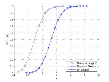
Figure 1: Simulated and theoretical CDFs of the regulated test statistics under $\mathcal{S}_{0}$: Real-valued case, MED with $N=1000$.

We next evaluate the accuracy of threshold setting for the CND detection using the formula in Section IV. Fig. 2 shows the threshold values at different probability of false alarms for real-valued case with $N=10000$. For comparison, the true thresholds (based on simulations) and the thresholds by using the theory for large $K$ in [5] are also included in the figure. The proposed theory based on fixed $K$ is much more accurate than the theory in [5] and gives the threshold values approaching to the true values.

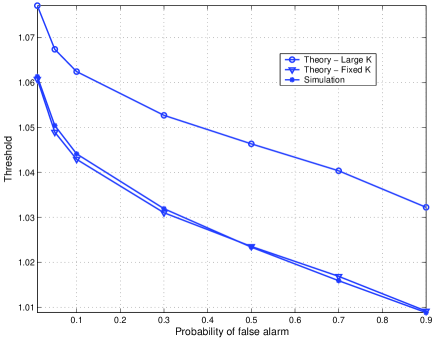
Figure 2: Comparison of threshold values under $\mathcal{S}_{0}$: Real-valued case, CND with $N=10000$.

VI-B Scenario $\mathcal{S}_{1}$

We then compare the detection probability results predicted by the formulas derived in this paper and reference [5] with large $K$ assumption. The probabilities of detection for CND by using simulations and different theoretical formulas are shown in Fig. 3 with $N=10000$ and SNR = $-15$dB (real-valued case). For a target probability of false alarm, we first use simulations to determine the decision threshold, then obtain the probability of detection based on simulations or the related formulas. Again, the proposed formula based on fixed $K$ is much more accurate than the formula in [5] and gives the values approaching to the true values. From Fig. 3, it is also seen that, interestingly, for a target probability of false alarm, the probability of detection predicted by our method tends to be conservative, which seems to be good to primary users in terms of protection requirement. Finally, as the results derived in this paper are asymptotic, they will approach the simulated ones more accurately when the sample size increases.

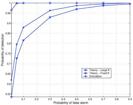
Figure 3: Comparison of estimations for probability of detection under $\mathcal{S}_{1}$: Real-valued case, CND with $N=10000$ and SNR = $-15$dB.

VII Conclusions

In this paper, theoretic distributions of the test statistics for some eigenvalue based detections have been derived for any fixed $K$ but large $N$, from which the probability of detection and probability of false alarm have been obtained. The results are useful in practice to determine the detection thresholds and predict the performances of the sensing algorithms. Extensive simulations have shown that theoretic results have higher accuracy than existing stuties.

References

- [1] S. Haykin, “Cognitive radio: Brain-empowered wireless communications,” IEEE J. Selected Areas in Communications, vol.23, No.2, pp.201–220, Feb. 2005.
- [2] Y.-C. Liang, Y. Zeng, E.C.Y. Peh and A.T. Hoang, “Sensing-throughput tradeoff for cognitive radio networks”, IEEE Trans. Wireless Communications, vol.7, no.4, pp.1326–1337, April 2008.
- [3] Y. Zeng, Y.-C. Liang, A. T. Hoang, and R. Zhang “A review on spectrum sensing for cognitive radio: challenges and solutions,” EURASIP Journal on Advances in Signal Processing, Article Number: 381465, 2010.
- [4] R. Tandra, and A. Sahai, “SNR walls for signal detection,” IEEE Journal of Selected Topics in Signal Processing, vol. 2, pp. 4–17, Feb. 2008.
- [5] Y. Zeng and Y.-C. Liang, “Eigenvalue based spectrum sensing algorithms for cognitive radio,” IEEE Trans. Communications, vol.57, no.6, pp.1784–1793, June 2009.
- [6] Y. Zeng and Y.-C. Liang, “Eigenvalue based sensing algorithms,” Available at www.ieee802.org/22, doc. no: IEEE 802.22-06/0119r0, July 2006.
- [7] R. Zhang, T. J. Lim, Y.-C. Liang, and Y. Zeng “Multi-antenna based spectrum sensing for cognitive radios: A GLRT approach,” IEEE Trans. Communications, vol.58, no.1, pp.84–88, Jan. 2010.
- [8] Y. Zeng, C. L. Koh and Y.-C. Liang, “Maximum eigenvalue detection: Theory and application,” in Proc. of IEEE International Conference on Communications (ICC), Beijing, China, May 2008.
- [9] L. Cardoso, M. Debbah, P. Bianchi, and J. Najim, “Cooperative spectrum sensing using random matrix theory,” in Proc. 3rd International Symposium on Wireless Pervasive Computing (ISWPC) , May 2008, pp.334–338.
- [10] F. Penna, R. Garello, and M. A. Spirito, “Cooperative spectrum sensing based on the limiting eigenvalue ratio distribution in wishart matrices,” IEEE Communications Letters, vol.13, no.7, pp.507–509, July 2009.
- [11] I. M. Johnstone, “On the distribution of the largest eigenvalue in principle components analysis,” The Annals of Statistics, vol.29, no.2, pp.295–327, 2001.
- [12] Z.D. Bai, Z. Fang and Y.C. Liang, Spectral Theory of Large Dimentional Random Matrices and its Applications in Wireless Commnications and Finance Statistics, USTC Press, China, 2009.
- [13] F. Penna, R. Garello, D. Figlioli, and M. A. Spirito, “Exact non-asymptotic threshold for eigenvalue-based spectrum sensing,” in Proc. CrownCom, 2009.
- [14] T.W. Anderson, “Asymptotic theory for principal component analysis,” Ann. Math. Stat. 122-148, 1963.
- [15] V.V. Petrov, Sums of Independent Random Variables, Springer-Verlag, New York, 1975.
- [16] Y.-C. Liang, G. Pan, and Y. Zeng, “On the performance of spectrum sensing algorithms using multiple antennas,” IEEE Trans. Wireless Communications, to be submitted, 2010.