Energy Spectra of Quantum Turbulence: Large-scale Simulation and Modeling

Abstract

In $2048^{3}$ simulation of quantum turbulence within the Gross-Pitaevskii equation we demonstrate that the large scale motions have a classical Kolmogorov-1941 energy spectrum $E(k)\propto k^{-5/3}$, followed by an energy accumulation with $E(k)\simeq$ const at  $k$ about the reciprocal mean intervortex distance. This behavior was predicted by the L’vov-Nazarenko-Rudenko bottleneck model of gradual eddy-wave crossover [J. Low Temp. Phys., 153, 140-161 (2008)], further developed in the paper.

I Introduction

Hydrodynamic turbulence (HD) Frisch – loosely defined as a random behavior of fluids – remains the most important unsolved problem of classical physics, as was pointed out by Richard Feynman.

Quantum turbulence (QT) – a trademark of turbulence in superfluid ³He, ⁴He and in Bose-Einshtein condensates of cold atomic vapors VD – has added a new twist in the turbulence research shading light on old problems from a new angle. QT consists of a tangle of quantized vortex lines with a fixed core radius $a_{0}$ and a finite (quantized) velocity circulation $\kappa=h/M$, where $M$ is the proper atomic mass VD . The superfluid has zero viscosity, and in the zero-temperature limit, which is the simplest for theoreticians and reachable for experimentalists exp , the QT’s Reynolds number, Re, is infinite. This brings (at least, the zero-temperature) QT to a desired prototype for better insight in the classical HD turbulence.

The tangle of vortex lines in QT is characterized by a mean intervortex distance, $\ell$. For large $R$-scale motions with $R\gg\ell$ the vortex tangles are better understood as bundles of nearly parallel vortex lines with mean curvature of about $R$ VD . For large scales the quantization of vortex lines can be neglected and QT can be considered as the classical one, in which the energy density in the $k$-space, $E(k)$, is given by the celebrated Kolmogorov-1941 (K41) law K41 :

$$E_{\scriptscriptstyle\rm{K41}}(k) = C\,{\varepsilon^{2/3}}{k^{-5/3}}\,,$$ (1)

$$E({\bm{r}}) \equiv {\left\langle|{\bm{u}}({\bm{r}})|^{2}\right\rangle}/{2}=\!\!\int\!\!E(k)dk\,,$$

confirmed experimentally and numerically Frisch . Here $C\sim 1$, $\varepsilon$ is the energy flux over scales, and $E({\bm{r}})$ is the energy density of turbulent velocity fluctuations per unit mass. Kelvin waves (KWs) are helix-like deformations of vortex lines with wavelength $\lambda$: $a_{0}\!<\!\lambda\!<\!\ell$. Interactions of KWs on the same vortex line, but with different $k\sim\lambda^{-1}$ lead to the turbulent energy transfer toward large $k$. This idea (Svistunov Svistunov95 ) was developed and confirmed theoretically and numerically by Vinen et al. Vinen03 , Kozik–Svistunov (KS) KS and L’vov-Nazarenko (LN) LN . Two versions of KW spectrum where suggested in Refs. [KS, ; LN, ]:

$$E_{\scriptscriptstyle\rm{KS}}(k) = C_{\scriptscriptstyle\rm{KS}}\Lambda\,\varepsilon^{1/5}\kappa^{7/5}\,\ell^{-8/5}k^{-7/5},\ ~{}~{}~{}~{}~{}\mbox{KS,}$$ (2a)

$$E_{\scriptscriptstyle\rm{LN}}(k) = C_{\scriptscriptstyle\rm{LN}}\Lambda\,\varepsilon^{1/3}\kappa\,\Psi^{-2/3}\ell^{-4/3}k^{-5/3},\ \ \mbox{LN},$$

$$\Lambda\equiv\ln(\ell/a_{0})\,,$$

Here $C_{\scriptscriptstyle\rm{KS}}\gg 1$, $C_{\scriptscriptstyle\rm{LN}}\simeq 1/\pi$ (Ref. LLPN-11, ), and $\Psi<1$ characterizes the ratio of $\ell$ to the large-scale modulation of the vortex lines. Parameter $\Lambda\simeq 12\div 15$ in typical experiments in ³He and ⁴He exp . The choice between Eqs. (2) is under intensive debates LN-debate1 ; LN-debate2 ; LN-debate3 ; KS-debate , which, however, has no principle effect on issues discussed in this paper.

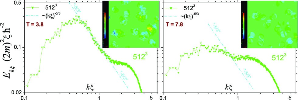
Figure 1: Color online. The incompressible energy spectra at time T=3.8. Right: the same as the left ones but at later time T=7.8. The color insets show vorticity 2D slice maps (see text for the definition). The grid size is $512^{3}$ and $\Lambda\simeq 1.5$.

The nature of energy transfer and energy spectrum is under intensive debates, too. Considering the inertial (Re$\rightarrow\infty$) energy transfer at the crossover scale $k\sim\ell^{-1}$, L’vov-Nazarenko-Rudenko (LNR) pointed out LNR1 that for $k\sim\ell^{-1}$ and $\Lambda\gg 1$ the KWs have much larger energy (2) than the HD energy (1) at the same energy flux $\varepsilon$. As the result LNR predicted a bottleneck energy accumulation around $k\sim\ell^{-1}$. On contrary, KS suggested Kozik08 an alternative scenario due to possible dominance of vortex-reconnections in the energy transfer at $k\sim\ell^{-1}$ without any energy stagnation. In Ref. [LNR2, ] LNR predicted two thermal-equilibrium regions between the HD (1) and KW (2) energy-flux spectra: with equipartition of the HD energy, $E(k)\propto k^{2}$, followed by equipartition of KW energy, $E(k)\simeq$const.

The direct numerical simulations (DNS) of QT mostly use the Gross-Pitaevskii equation (GPE) GP , which in dimensionless form is given by

$$2\,i\partial\psi/\partial t+\nabla^{2}\psi=g|\psi|^{2}\psi\ .$$ (3)

The macroscopic wave function $\psi({\bm{r}},t)$ plays a role of the complex order parameter, and $g$ is the coupling constant. The transformation $\psi=\sqrt{\rho}\,e^{i\theta}$ maps Eq. (3) to the Euler equation for ideal compressible fluid of density $\rho$ and velocity ${\bm{u}}={\bm{\nabla}}\theta$, and an extra quantum pressure term.

The numerical study of QT by GPE (3) has been reported in a few papers so far. Nore et al. Nore97 solved the GPE with resolutions up to 512³ and observed that as the quantized vortices became tangled, the incompressible kinetic energy spectra seemed to obey the K41 law (1) for a short period of time, but eventually deviated from it. Kobayashi and Tsubota KT05 solved the GPE on $256^{3}$ grid with an extra dissipation term at small scales, and showed the K41 law (1) more clearly. Yepez et al. Yepez09 simulated the GPE on grids up to 5760³ by using a unitary quantum lattice gas algorithm. They also found a spectrum $E(k)\propto k^{-5/3}$ and interpreted it as the K41 law (1) of HD turbulence. However, due to the choice of initial conditions, their simulation should correspond to the pure KW region $k>\ell^{-1}$ (thus supporting the LN-spectrum (2) of KWs).

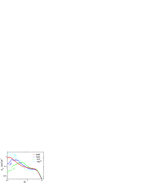
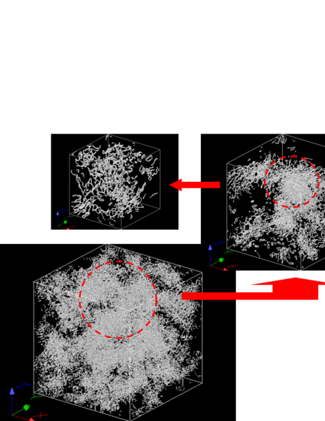
Figure 2: Color online. Left: Simulation results of the incompressible energy spectra $E(k\xi)$ normalized by ${\hbar^{2}/(4m^{2}\xi)}$. Symbols: $2048^{3}$ (${\color[rgb]{1,0,0}-\bullet-}$), $1024^{3}$ (${\color[rgb]{0,0,1}-\blacktriangle-}$), $512^{3}$ (${\color[rgb]{0,0.6,0}-\blacktriangledown-}$). $\Lambda$ varies from $\Lambda\simeq 1.5$ (slightly depending on time) for $512^{3}$ to $\Lambda\simeq 2.2$ for $2048^{3}$. Left: Dot-dashed (cyan) line: K41 “$-5/3$” scaling. A snapshot of vortex lines at the fully-developed turbulent state of $2048^{3}$ demonstrates the self-similarity of the bundle-vortex structure (see the dotted circles representing the zoom regions which vortex distributions are shown subsequently), typical for fully developed turbulence.

In the present paper, we solved the GPE on the grids up to $2048^{3}$ by parallelizing the simulation code on the Earth Simulator ES . In contrast to Ref. [Yepez09, ] we focused on HD- and crossover-regions, $k\lesssim\ell^{-1}$.
First, we confirmed the K41-law (1) in the HD-region of about two decades long, which is wider than that of any previous work.
Second, the visualization of vortices clearly shows the bundle-like structure, which has never been confirmed in GPE simulations on smaller grids.
Third, we discovered a plateau in the crossover region, $k\ell\gtrsim 2\pi$, further explained as the KW’s energy equipartition in the framework of the LNR’s bottleneck model LNR2 , which is revised here to account for the recently predicted LN and numerically observed Yepez09 LN spectrum (2) of KWs.

We consider this correspondence as a support in favor of LNR bottleneck theory, understanding, nevertheless, that interpretation of numerical (or experimental) data with the help of a theoretical model on the edge of its applicability (here $\Lambda\sim 1$) is often problematic, being a question of experience, physical intuition and taste. Currently we cannot fully exclude the alternative KS-scenario Kozik08 , even though it gives no energy stagnation for $\Lambda\gg 1$. More theoretical studies, numerical and laboratory experiments are required to fully understand the vortex dynamics in the crossover region of scales.

II Numerical procedure and results

In DNS we follow techniques KT05 but extend the maximum computational grid size from $256^{3}$ up to $2048^{3}$. The initial state is prepared by distributing random numbers created inside a range from $-N\pi\alpha$ to $N\pi\alpha$ into the phase $\theta({\bf r})$ on selected points $M^{3}$ $(M\ll N)$ and interpolating them to make a smooth velocity field on all grid points. Here $N$ is the total number of grid points and $\alpha$ is a control parameter for the initial energy input. Also, following KT05 we add to the GPE an effective artificial energy damping for small-scale motions by replacing in the Fourier transform of GPE $i\rightarrow i+1$ for $k_{x},\ k_{y},\ k_{z}>2\pi/\xi$, where $\xi\simeq a_{0}$ is the condensate coherence length.

GPE conserves the total number of particles and the total energy (Hamiltonian) of the system GP . We decompose Nore97 ; PRA the total energy density into the internal, $E_{\text{int}}\equiv g(\rho-1)^{2}/4$, the quantum, $E_{\text{qnt}}\equiv|{\bm{\nabla}}\sqrt{\rho}|^{2}/2$, and the kinetic, $E\equiv\rho|{\bm{u}}|^{2}/2$, energy densities. The kinetic energy is decomposed into compressible and incompressible components, both of which are monitored. Two typical spectra of the incompressible component are plotted in Fig. 1 with corresponding vortex distributions. The plot illustrates a $512^{3}$ run at times $3.8$ and $7.8$ in the left and right panels, respectively . The time evolution of the equation is calculated by a symplectic integral method, and a typical pseudo-spectral method is employed for the calculation of the kinetic energy term. The method is a standard one, which is known to guarantee sufficiently high accuracy for hydrodynamics simulations. In Fig. 1, left, one finds that the major part of the energy spectrum fits the K41 law (1) like in KT05 , but with the large inertial interval.

As expected, we also observed tangled vortex bundles clearly demonstrated in the insets of Fig. 1 showing a $x$-$y$ 2D slice of the polarization field’s color map, which is defined by summing up vortices ($\pm 1$) inside plaquettes lying within a constant radius ($=32\Delta x$) from a grid point. On the other hand, Fig. 1 is a typical example of a considerably decayed state, in which the main feature is rather small vortex rings distributed almost equally inside the simulation cubic region.

An important observation (Fig. 1) is a plateau-like region for $k\xi\gtrsim 1.5$ – a definite pile-up over the K41 spectrum – a clear manifestation of the energy stagnation.

The main numerical result of the present paper is Fig. 2. The left panel shows an inter-comparison of the incompressible kinetic energy spectrum $E(k)$ among $512^{3}$, $1024^{3}$ and $2048^{3}$ simulations. The K41 scaling (1) (shown as (cyan) dash-dotted lines) is extended to lower $k$ range with the grid-size increase. This is the first clear demonstration of the classical K41 scaling characteristic for the normal-fluid turbulence but maintained in the large-scale range of the superfluid turbulence. The visible extend of the K41 scaling on $2048^{3}$ grid is much larger than that in all previous simulations.

The right panel of Fig. 2 displays self-similar large structures of tangled vortices in the fully turbulent state: the large-scale vortex bundles in the maximum size, $2048^{3}$, and smaller self-similar tangled structures inside this cubic region in the subsequent insets.

Before discussion of these results we will revise shortly in the next Section the LNR model of the bottleneck crossover LNR2 to accont for recently predicted LN spectrum of Kelvin waves LN .

III LNR model of the bottleneck crossover

To find theoretically $E(k)$ we, following LNRLNR2 , approximate the superfluid motions as a mixture of “pure” HD- and KW-motions with the spectra $E^{{}^{\text{HD}}}\!(k)\equiv g(k\ell)E(k)$ and $E^{{}^{\text{KW}}}\!(k)\equiv[1-g(k\ell)]E(k)$. Here $g(k\ell)$ is the “blending” function, which was found in Ref. [LNR2, ] by calculation of energies of correlated and uncorrelated motions produced by a system of $\ell$-spaced wavy vortex lines:
$\displaystyle g(x)=g_{0}[0.32\ln(\Lambda+7.5)x]\,,\ g_{0}(x)=\Big{[}1+\frac{x^{2}\,\exp(x)}{4\pi(1+x)}\Big{]}^{-1}$.

The total energy flux, $\varepsilon_{k}$, also consisting of HD and KW contributions LNR2 , is modeled by dimensional reasoning in the differential approximation. Hence, for $k\to 0$ the energy flux is purely HD and thus $\varepsilon_{k}\propto k^{-2}\sqrt{E^{{}^{\text{HD}}}}dE^{{}^{\text{HD}}}\!\!/dk$. From the other side, for $k\to\infty$ the energy flux is purely KW and thus $\varepsilon_{k}\propto[E^{{}^{\text{KW}}}]^{2}dE^{{}^{\text{KW}}}\!\!/dk$. Important that in contrast to the Ref. [LNR2, ], where the physically irrelevant KS-spectrum of KWs (2a) was used, we employ here the proper LN-spectrum (2) that accounts for large-scale vortex-line modulations with short KWs LN . The full equation for the total energy flux reads:

$$-\Big{\{}\frac{1}{8}\sqrt{k^{11}g(k\ell){E}(k)}+\frac{3}{5}\frac{\big{\{}\Psi k^{3}k_{*}\,\ell^{2}[1-g(k\ell)E(k)]\big{\}}^{2}}{\big{(}C_{\scriptscriptstyle\rm{LN}}\Lambda\,\kappa\big{)}^{3}}\Big{\}}$$

$$\times\frac{d}{dk}\Big{\{}{E}(k)\Big{[}\frac{g(k\ell)}{k^{2}}+\frac{1-g(k\ell)}{k_{*}^{2}}\Big{]}\Big{\}}=\varepsilon_{k}\ .~{}~{}~{}~{}~{}~{}~{}~{}~{}~{}~{}~{}~{}~{}$$ (4)

Here $E^{{}^{\text{HD}}}\!(k_{*})\!=\!E^{{}^{\text{KW}}}\!(k_{*})\,,\,\Rightarrow\,k_{*}\ell\simeq 6.64/\ln(\Lambda+7.5)$. In the inertial range the energy flux is constant $\varepsilon(k)=\varepsilon$. Moreover, in the system of quantum filaments it is related to the rms vorticity $\sqrt{\left\langle|\bm{\omega}|^{2}\right\rangle}\simeq\kappa/\ell^{2}$ via $\left\langle|\bm{\omega}|^{2}\right\rangle=2\int{k^{2}E(k)dk}$ (see Refs. [Frisch, ; VD, ]). This allows to find solutions of Eq. (4) for different $\Lambda$ as depicted in the Fig. 3 by (black) dashed and solid curves .

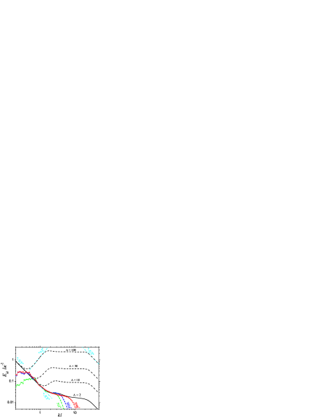
Figure 3: Color online. Incompressible energy spectra plotted vs. $k\ell$ and normalized by $\kappa^{2}/\ell$. The simulation results (the same symbols) and the LNR model for $\Lambda=10,30,100$ [dashed (black) curves] are brought together to the theoretical [solid (black)] curve with $\Lambda=2$ by superposing the K41 (both simulations and model) and plateau regions (only for simulations). Dot-dashed (cyan) lines show different scaling asymptotics.

Four distinct scaling regions are evident ($\Lambda\gg 1$):

I. $k\ell\ll 1$: $E(k)$ and $\varepsilon_{k}$ are dominated by the “pure” HD contributions, and the K41 law (1) is revealed.

II. $k\ell\gg 1$: $E(k)$ and $\varepsilon_{k}$ are dominated by the “pure” KW contributions, and one observes the LN spectrum (2) of KWs with a constant energy flux.

III. $k\lesssim k_{*}$: As explained above, for $\Lambda\gg 1$ the KW turbulence is much less efficient in the energy transfer over scales than its HD counterpart with the same energy, which leads to the (HD) energy accumulation with a level $E(k)\approx E^{{}^{\text{HD}}}\!(k)\gg E_{\scriptscriptstyle\rm{K41}}(k)$. For $k\lesssim k_{*}$, both $E(k)$ and $\varepsilon_{k}$ are still dominated by HD contributions, but the energy flux is much smaller than the K41 estimate requires. This is like a flux-free HD system, thus, the thermodynamic equilibrium is expected with the equipartition of energy between the degrees of freedom: 3D-energy spectrum is constant, hence, the 1D energy spectrum $E^{{}^{\text{HD}}}(k)\propto k^{2}$. This scaling is observed in Fig. 3, middle, for $k\lesssim k_{*}$. Think of a lake before a dumb, where the water velocity being much smaller than that in the source river does not effect on the water level, which is practically horizontal. This interpretation of the energy bottleneck effect as “incomplete thermalization” (of only high $k$ region) was suggested by Frisch et. al. Fri08 .

IV. $k\gtrsim k_{*}$: Unexpectedly, we observe here almost a $k$-independent 1D-energy spectrum, $E(k)\!\approx$ const, inherent to the thermodynamic equilibrium of KWs. In the “pure” KW system, such a spectrum shows up for $k\gg k_{*}$. However, in the region IV, the energy of the system is already dominated by the KW contributions, $E(k)\approx E^{{}^{\text{KW}}}\!(k)$, while the energy flux is still dominated by the HD-motions LNR2 . Hence, this is almost a flux-free system of KWs, which is indeed found in the thermodynamic equilibrium with the 1D energy equipartition: $E(k)^{{}^{\text{KW}}}\!\!=$ const.

As one sees from Fig. 3 with the decrease of $\Lambda$ the pile-up becomes less pronounced. For $\Lambda=2$ the equilibrium HD region (III) almost disappeared, however the equilibrium KW region (IV) is still well pronounced being much less sensitive to the value of $\Lambda$.

IV Discussion and summary

IV.1 Classical and quantum energy bottleneck effects

The bottleneck effect in classical hydrodynamic turbulence is understood traditionally VD07 ; 4096 as a hump on a plot of compensated energy spectrum $E(k)k^{5/3}$ in the crossover region between inertial and viscous intervals. This is very general phenomenon reported in many numerical simulations and experiments of classical hydrodynamic turbulence. For example, Yeung and Zhou 2 , Gotoh et al 3 , Kaneda et al 4 and Dobler et al 5 found the bottleneck effect in their numerical simulations. Saddoughi and Veeravalli 6 studied the energy spectrum of atmospheric turbulence and reported the bottleneck effect. Shen and Warhaft 7 , Pak et al 8 , She and Jackson9 and other experimental groups also observed the bottleneck effect in fluid turbulence. The bottleneck effect has been seen in other forms of turbulence as well, see e.g. Refs. [10-15] in Ref. [VD07, ].

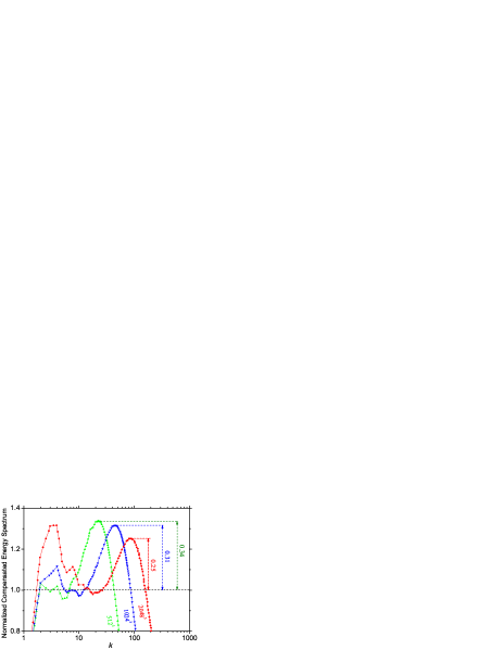
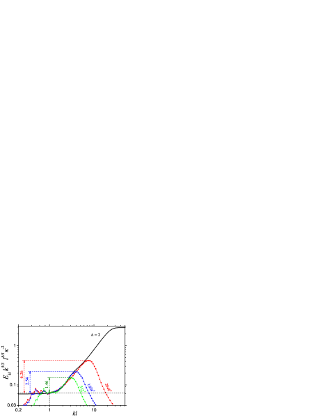
Figure 4: Color online. Comparison of the compensated energy spectra, $E(k)\,k^{5/3}$ (the same color-symbol code as in previous figures), and of the bottleneck magnitudes $M_{\text{bn}}$ (dashed color arrows). Left: DNS data of classical hydrodynamic turbulence VD07 (cf. Figure 1 in Ref. VD07, ): modest values of $M_{\text{bn}}\lesssim 1.34$ decrease with the increase of the resolution. Right: Our DNS data of quantum superfluid turbulence: large values of $M_{\text{bn}}$ increase with the resolution up to $M_{\text{bn}}\simeq 6.26$.

To characterize the value of this effect one can introduce a “bottleneck magnitude” $M_{\text{bn}}$: the hump height, normalized by the plateau value of $E(k)k^{5/3}$ in the inertial interval. For example, in high resolution DNS of the classical hydrodynamic turbulence VD07 , shown in Fig. 4, left, its magnitude $M_{\text{bn}}\simeq 0.34$ for 512³ DNS and decreases with the resolution increase: $M_{\text{bn}}\simeq 0.31$ for $1024^{3}$ and $M_{\text{bn}}\simeq 0.25$ for $2048^{3}$. Recent results 4096 based on the $4096^{3}$ DNS confirm the statement that the bottleneck magnitude in classical turbulence systematically decreases with the DNS resolution increase (or equivalently, with the Taylor-Reynolds number Re_λ growth, and $M_{\text{bn}}\to\mathrm{Re}_{\lambda}^{-0.4}$ as Re${}_{\lambda}\to\infty$).

Coming to comparison of the bottleneck effects in our modeling and numerical simulations we should notice that the LNR model accounts only for leading in $\Lambda=\ln(\ell/a_{0})$ terms LNR1 ; LNR2 . Moreover, it is based on the differential approximation for the energy flux, which is reasonable for vivid power-like behavior of the energy spectra, which exists only for $\Lambda\gg 1$, Fig. 3. Therefore, one expects that the LNR model is suitable for quantitative analysis of experiments in ³He and ⁴He, where $\Lambda\simeq 12\div 15$, and can only qualitatively describe the simulations presented here with $\Lambda\simeq 2$.

Nevertheless, the simulations clearly demonstrate in Fig. 3 the plateau that immediately follows the K41-scaling (1), which agrees with the LNR model prediction for $\Lambda\simeq 2$ (Fig. 3). The plateau broadens with the grid-size increase towards that of the LNR model curve (the earlier cutoff of the simulation data is due to the artificial dissipation). The resolution of the current simulations does not allow to resolve the KW-scaling (2) with constant energy flux as it was done in Yepez09 , but the bottleneck is definitely there.

To measure bottleneck magnitudes in quantum turbulence we re-plotted our data of Fig. 3, compensating $E(k)$ by K41 prediction, i.e. multiplying by $(k\ell)^{5/3}$, see Fig. 4, right. One sees large humps with magnitudes $M_{\text{bn}}$ that increases with the resolution, reaching $M_{\text{bn}}\simeq 6.26$ for $2048^{3}$. Recall that in the classical turbulence $M_{\text{bn}}$ is much (in about 20 times!) smaller and demonstrates opposite tendency with the resolution.

We concluded that classical and quantum bottlenecks have completely different nature. Small magnitude of the bottleneck in classical turbulence is related to some nonlocality of the energy transfer toward small scales that is slightly suppressed due to fast decrease of the turbulence energy in the dissipation range, while in quantum turbulence (at zero temperature) the essential bottleneck effect originates from the strong suppression of the energy flux in the Kelvin wave region.

Indeed, Fig. 4, right, demonstrates a good agreement between the QT DNS data and the LNR model prediction (that accounts for the flux suppression mentioned above) for $\Lambda\simeq 2$, which improves with increasing the DNS resolution. The cutoff of the spectra for large $k$ is a consequence of limited $k$-space in the simulations. One predicts that with the further increase of the resolution the bottleneck magnitude can reach $M_{\text{bn}}\simeq 50$ at $\Lambda\simeq 2$ and even much larger values for larger $\Lambda$.

IV.2 Summary

In the paper we conclude that the observed essential bottleneck energy accumulation has definitely quantum nature (quantization of circulation) and can be completely rationalized within the LNR model of gradual eddy-wave crossover, suggested in Ref. [LNR2, ]. We consider this model as a Minimal Model of Quantum Turbulence that describes homogeneous isotropic turbulence in superfluids with energy pumped at scales much larger than the mean intervortex distance, and reveals reasonable (and even unexpectedly good) agreement with the simulations of Gross-Pitaevskii equation discussed here. The reason is that in the most questionable crossover region, the LNR model predicts a local thermodynamic equilibrium, where the energy spectra are universal and non-sensitive to the details of microscopic mechanisms of interactions, e.g. vortex-reconnections, etc.

Acknowlegements

We acknowledge the partial support of a Grants-in Aid for Scientific Research from JSPS # 21340104 and from MEXT # 17071008, of the Japan Society for the Promotion of Science grant # S-09147, of the EU Research Infrastructures under the FP7 Capacities Specific Programme, MICROKELVIN (project # 228464) and of the U.S. - Israel BSF (grant # 2008110).

References

- (1) U. Frisch, Turbulence, (Cambridge University Press, Cambridge, 1995).
- (2) W.F. Vinen, R.J. Donnelly, Physics Today, 60, 43 (2007).
- (3) V.B. Eltsov, R. de Graaf, R. Hanninen, M. Krusius, R.E. Solntsev, V.S. L’vov, A.I. Golov, P.M. Walmsley, Progress in Low Temperature Physics XVI, pp. 46-146 (2009).
- (4) A.N. Kolmogorov, Dokl. Akad. Nauk SSSR 30, 301 (1941) and 31, 538 (1941), [reprinted in Proc. Roy. Soc. A 434, 9 (1991) and 434, 15(1991) ].
- (5) B.V. Svistunov, Phys. Rev. B 52, 3647 (1995).
- (6) W.F. Vinen, M. Tsubota, M. Mitani, Phys. Rev. Lett. 91, 135301 (2003).
- (7) E. Kozik, B.V. Svistunov, Phys. Rev. Lett. 92, 035301 (2004); Phys. Rev. Lett. 94, 025301 (2005); Phys. Rev. B 72, 172505 (2005).
- (8) V.S. L’vov, S. Nazarenko, Pisma v ZhETF, 91, 464 (2010).
- (9) J. Laurie, V.S. L’vov, S. Nazarenko, O. Rudenko, Phys. Rev. B., 81, 104526 (2010);
- (10) V.V. Lebedev, V.S. L’vov, J. of Low Temp. Phys, 161, 548-554 (2010)
- (11) V.V. Lebedev, V.S. L’vov, S.V. Nazarenko, J. of Low Temp. Phys, 161, 606-610 (2010)
- (12) E. Kozik, B.V. Svistunov, Phys. Rev. B 82, 140510(R) (2010);
- (13) V.S. L’vov, S.V. Nazarenko, O. Rudenko, Phys. Rev. B 76, 024520 (2007).
- (14) E. Kozik, B.V. Svistunov, Phys. Rev. B 77, 060502 (2008) and Phys. Rev. Letts. 100, 195302 (2008).
- (15) V.S. L’vov, S.V. Nazarenko, O. Rudenko, Journal of Low Temp. Phys., 153, 140-161 (2008)
- (16) L. Pitaevskii and S. Stringari, Bose-Einstein Condensation, (Oxford University Press, USA, 2003).
- (17) C. Nore, M. Abid, and M. E. Brachet, Phys. Rev. Lett. 78, 3896 (1997); Phys. Fluids 9, 2644 (1997).
- (18) M. Tsubota, J. Phys. Soc. Jpn. 77, 111006 (2008).
- (19) M. Kobayashi, M. Tsubota, Phys. Rev. Lett. 94, 065302 (2005); J. Phys. Soc. Jpn. 74, 3248 (2005).
- (20) R. Numasato, M. Tsubota, V.S. L’vov, Phys. Rev. A 81, 063630 (2010).
- (21) J. Yepez, G. Vahala, L. Vahala, M. Soe, Phys. Rev. Lett. 103, 084501 (2009).
- (22) Earth Similator is a vector-parallel machine, described at http://www.jamstec.go.jp/esc/index.en.html
- (23) M.K. Verma, D. Donzis, J. Phys. A: Math. Theor. 40, 4401 (2007).
- (24) D. Donzis and K.R. Sreenivassan, J. Fluid Mech. 657, 171-188, (2010).
- (25) U. Frisch et. al., Phys.Rev. Letts, 101, 144501 (2008)
- (26) L. Boue, R. Dasgupta, J. Laurie, V.S. L’vov, S. Nazarenko and I. Procaccia, arXiv:1103.5967
- (27) Yeung P K and Zhou Y, Rev. E 56 1746 (1997).
- (28) Gotoh T, Fukayama D and Nakano T, Phys. Fluids 14 1065 (2002).
- (29) Kaneda Y, Ishihara T, Yokokawa M, Itakura K and Uno A, Phys. Fluids 15 L21 (2003)
- (30) Dobler W, Haugen N E L, Yousef T A and Brandenburg A, Phys. Rev. E 68 26304 (2003).
- (31) Saddoughi S G and Veeravalli S V, J. Fluid Mech. 268 333 (1994).
- (32) Shen X and Warhaft Z, Phys. Fluids 12 2976 (2000)
- (33) Pak H K, Goldburg W I and Sirivat A,Fluid Dyn. Res. 8 19 (1991)
- (34) She Z S and Jackson E, Phys. Fluids A 5 1526 (1993)