The Casimir force of Quantum Spring in the (D+1)-dimensional spacetime

Abstract

The Casimir effect for a massless scalar field on the helix boundary condition which is named as quantum spring is studied in our recent paperFeng . In this paper, the Casimir effect of the quantum spring is investigated in $(D+1)$-dimensional spacetime for the massless and massive scalar fields by using the zeta function techniques. We obtain the exact results of the Casimir energy and Casimir force for any $D$, which indicate a $Z_{2}$ symmetry of the two space dimensions. The Casimir energy and Casimir force have different expressions for odd and even dimensional space in the massless case but in both cases the force is attractive. In the case of odd-dimensional space, the Casimir energy density can be expressed by the Bernoulli numbers, while in the even case it can be expressed by the $\zeta$-function. And we also show that the Casimir force has a maximum value which depends on the spacetime dimensions. In particular, for a massive scalar field, we found that the Casimir force varies as the mass of the field changes.

I Introduction

The work done by CasimirCasimir:1948dh more than 60 years ago starts an important research field as one of the direct manifestations of the existence of the zero-point vacuum oscillations. The Casimir effect has now been extensively studied both in experiment and theory, especially in the past decade due to the precise verification benefited from the applications of the modern laboratory techniquesklimchitskaya . And it is still a topic full of life that attracted increasing interests in both fundamental and applied sciencePlunien:1986ca . The Casimir effect, in its simplest form, is the attraction between two plane-parallel uncharged perfectly conducting plates in vacuum.

The nature of the Casimir force may depend on (i) the background field, (ii) the spacetime dimensionality, (iii) the type of boundary conditions, (iv) the topology of spacetime, (v) the finite temperature. The most evident example of the dependence on the geometry is given by the Casimir effect inside a rectangular box Plunien:1986ca ; Lukosz . The detailed calculation of the Casimir force inside a D-dimensional rectangular cavity was shown in Li , in which the sign of the Casimir energy depends on the length of the sides. The Casimir force arises not only in the presence of material boundaries, but also in spaces with nontrivial topology. For example, we get the scalar field on a flat manifold with topology of a circle $S^{1}$. The topology of $S^{1}$ causes the periodicity condition $\phi(t,0)=\phi(t,C)$, where $C$ is the circumference of $S^{1}$, imposed on the wave function which is of the same kind as those due to boundary. Similarly, the antiperiodic conditions can be drawn on a Möbius strip. The $\zeta$-function regularization procedure is a very powerful and elegant technique for the Casimir effect. Rigorous extension of the proof of Epstein $\zeta$-function regularization has been discussed in Elizalde . Vacuum polarization in the background of on string was first considered in Helliwell:1986hs . The generalized $\zeta$-function has many interesting applications, e.g., in the piecewise string Li:1990bz . Similar analysis has been applied to monopoles BezerradeMello:1999ge , p-branes Shi:1991qc or pistons Zhai .Recently,the Casimir effect has been paid more attention due to the development of precise measurements Decca:2007yb , and it has been applied to the fabrication of microelectromechanical systems (MEMS)MEMS . Furthermore, some new methods have developed for computing the Casimir energy between a finite number of compact objects Emig:2007cf . In our recent paper, the Casimir effect for a massless scalar field on the helix boundary condition is investigated by using the zeta function techniquesFeng . We find that the Casimir force is very much like the force on a spring that obeys the hooke’s law in mechanics. However, in this case, the force comes from a quantum effect, and so we would like to call this structures as a quantum springFeng . On the other hand, the Casimir effect for the massive scalar field is also studied by some authorsBordag2 . As is known that the Casimir effect disappears as the mass of the field goes to infinity since there are no more quantum fluctuations in the limit. But the precise way the Casimir energy varies as the mass changes is worth studyingPlunien:1986ca .

In this paper, we study the quantum spring in ($D+1$)-dimensional spacetime. We obtain the exact results of the Casimir energy and Casimir force for the massless and massive scalar fields in the ($D+1$)-dimensional spacetime. The final results also tell us that there is a $Z_{2}$ symmetry of the two space dimensions. And we also show that the Casimir force has a maximum value which depends on the spacetime dimensions for both massless and massive cases. Especially, we show that the Casmir force varies as the mass of the field changes.

II Topology of the flat ($D$+1)-dimensional spacetime

As mentioned in Section I, the Casimir effect arises not only in the presence of material boundaries, but also in spaces with nontrivial topology. For example, we get the scalar field on a flat manifold with topology of a circle $S^{1}$. The topology of $S^{1}$ causes the periodicity condition $\phi(t,0)=\phi(t,C)$. Before we consider complicated cases in the flat spacetime, we have to discuss the lattices.

A lattice $\Lambda$ is defined as a set of points in a flat ($D+1$)-dimensional spacetime $\mathcal{M}^{D+1}$, of the form

$$\Lambda=\left\{~{}\sum_{i=0}^{D}n_{i}\mathbbm{e}_{i}~{}|~{}n_{i}\in\mathcal{Z}~{}\right\}\,,$$ (1)

where $\{\mathbbm{e}_{i}\}$ is a set of basis vectors of $\mathcal{M}^{D+1}$. In terms of the components $v^{i}$ of vectors $\mathbb{V}\in\mathcal{M}^{D+1}$, we define the inner products as

$$\mathbb{V}\cdot\mathbb{W}=\epsilon(a)v^{i}w^{j}\delta_{ij}\,,$$ (2)

with $\epsilon(a)=1$ for $i=0$, $\epsilon(a)=-1$ for otherwise. In the $x^{1}-x^{2}$ plane, the sublattice $\Lambda^{\prime\prime}\subset\Lambda^{\prime}\subset\Lambda$ are

$$\Lambda^{\prime}=\left\{~{}n_{1}\mathbbm{e}_{1}+n_{2}\mathbbm{e}_{2}~{}|~{}n_{1,2}\in\mathcal{Z}~{}\right\}\,,$$ (3)

and

$$\Lambda^{\prime\prime}=\left\{~{}n(\mathbbm{e}_{1}+\mathbbm{e}_{2})~{}|~{}n\in\mathcal{Z}~{}\right\}\,.$$ (4)

The unit cylinder-cell is the set of points

$$U_{c} = \bigg{\{}\mathbb{X}=\sum_{i=0}^{D}x^{i}\mathbbm{e}_{i}~{}|~{}0\leq x^{1}<a,-h\leq x^{2}<0,$$ (5)

$$-\infty<x^{0}<\infty,-\frac{L}{2}\leq x^{T}\leq\frac{L}{2}\bigg{\}}\,,$$

where $T=3,\cdots,D$. When $L\rightarrow\infty$, it contains precisely one lattice point (i.e. $\mathbb{X}=0$), and any vector $\mathbb{V}$ has precisely one ”image” in the unit cylinder-cell, obtained by adding a sublattice vector to it.

In this paper, we choose a topology of the flat ($D+1$)-dimensional spacetime: $U_{c}\equiv U_{c}+\mathbbm{u},\mathbbm{u}\in\Lambda^{\prime\prime}$. This topology causes the helix boundary condition for a Hermitian massless or massive scalar field

$$\phi(t,x^{1}+a,x^{2},x^{T})=\phi(t,x^{1},x^{2}+h,x^{T})\,,$$ (6)

where, if $a=0$ or $h=0$, it returns to the periodicity boundary condition.

III Massless scalar field

III.1 Casmir energy in the massless case

In calculations on the Casimir effect, extensive use is made of eigenfunctions and eigenvalues of the corresponding field equation. A Hermitian massless scalar field $\phi(t,x^{\alpha},x^{T})$ defined in the ($D+1$)-dimensional flat spacetime satisfies the free Klein-Gordon equation:

$$\left(\partial_{t}^{2}-\partial_{i}^{2}\right)\phi(t,x^{\alpha},x^{T})=0\,,$$ (7)

where $i=1,\cdots,D;\alpha=1,2;T=3,\cdots,D$. Under the boundary condition (6), the modes of the field are then

$$\phi_{n}(t,x^{\alpha},x^{T})=\mathcal{N}e^{-i\omega_{n}t+ik_{x}x+ik_{z}z+ik_{T}x^{T}}\,,$$ (8)

where $\mathcal{N}$ is a normalization factor and $x^{1}=x,x^{2}=z$, and we have

$$\omega_{n}^{2}=k_{T}^{2}+k_{x}^{2}+\left(-\frac{2\pi n}{h}+\frac{k_{x}}{h}a\right)^{2}=k_{T}^{2}+k_{z}^{2}+\left(\frac{2\pi n}{a}+\frac{k_{z}}{a}h\right)^{2}\,.$$ (9)

Here, $k_{x}$ and $k_{z}$ satisfy

$$ak_{x}-hk_{z}=2n\pi\,,(n=0,\pm 1,\pm 2,\cdots)\,.$$ (10)

In the ground state (vacuum), each of these modes contributes an energy of $\omega_{n}/2$. The energy density of the field in ($D+1$)-dimensional spacetime is thus given by

$$E^{D} =\frac{1}{2a}\int\frac{d^{D-1}k}{(2\pi)^{D-1}}\sum_{n=-\infty}^{\infty}\sqrt{k_{T}^{2}+k_{z}^{2}+\left(\frac{2\pi n}{a}+\frac{k_{z}}{a}h\right)^{2}}\,,$$

where we have assumed $a\neq 0$ without losing generalities. Eq.(LABEL:tot_energy) can be rewritten as

$$E^{D} =\frac{1}{2a\sqrt{\gamma}}\int\frac{d^{D-1}u}{(2\pi)^{D-1}}\sum_{n=-\infty}^{\infty}\sqrt{u^{2}+\left(\frac{2\pi n}{a\gamma}\right)^{2}}\,,$$

where we have defined

$$\gamma\equiv 1+\frac{h^{2}}{a^{2}}.$$ (13)

Using the mathematical identity,

$$\int_{-\infty}^{\infty}f(u)d^{D-1}u=\frac{2\pi^{\frac{D-1}{2}}}{\Gamma\left(\frac{D-1}{2}\right)}\int_{0}^{\infty}u^{D-2}f(u)du,$$ (14)

we get

$$\int d^{D-1}u\sqrt{u^{2}+\left(\frac{2\pi n}{a\sqrt{\gamma}}\right)^{2}}=\frac{\pi^{\frac{D-1}{2}}\Gamma\left(-\frac{D}{2}\right)}{\Gamma\left(-\frac{1}{2}\right)}\left(\frac{2\pi n}{a\sqrt{\gamma}}\right)^{D}\,.$$ (15)

thus the energy density in Eq.(LABEL:tot_energy) is reduced to

$$E^{D}=-\frac{\pi^{\frac{D}{2}}}{a^{D+1}\gamma^{\frac{D+1}{2}}}\Gamma\left(-\frac{D}{2}\right)\zeta(-D)\,,$$ (16)

where $\zeta(-D)$ is the Riemann $\zeta$ function.

In the case of $D=2j+1$, Eq.(16) shows directly the Casimir energy and the final expression is

$$E_{R}^{2j+1}=-\frac{(2\pi)^{j+1}|B_{2j+2}|}{(2j+1)!!(2j+2)(a^{2}+h^{2})^{j+1}}\,,$$ (17)

where $j=1,2,...$ and the Bernoulli numbers are $B_{2}=\frac{1}{6},B_{4}=-\frac{1}{30},B_{6}=\frac{1}{42},B_{8}=-\frac{1}{30},B_{10}=\frac{5}{66},B_{12}=-\frac{691}{2730},B_{14}=\frac{7}{6},B_{16}=-\frac{3617}{510},...$. In the case of $D=2j$, because $\Gamma(-j)$ is a pole of order 1, Eq.(16) should be regularized by using the reflection relation

$$\Gamma\left(\frac{s}{2}\right)\zeta(s)=\pi^{s-\frac{1}{2}}\Gamma\left(\frac{1-s}{2}\right)\zeta(1-s)\,.$$ (18)

Then, the final expression is

$$E_{R}^{2j}=-\frac{(2j-1)!!\zeta(2j+1)}{(2\pi)^{j}(a^{2}+h^{2})^{j+\frac{1}{2}}}\,.$$ (19)

Obviously, we have the symmetry of $a\leftrightarrow h$ in both cases. It is worth noting that the Casimir energy has different expressions for the odd and even space dimensions.

III.2 The Casimir force in the massless case

The Casimir force on the $x$ direction is given by

$$F_{a}=-\frac{\partial E_{R}^{D+1}}{\partial a}\,.$$ (20)

For the odd-dimensional space, the final expression for the Casimir force is

$$F_{a}^{2j+1}=-\frac{(2\pi)^{j+1}|B_{2j+2}|a}{(2j+1)!!(a^{2}+h^{2})^{j+2}},$$ (21)

which has a maximum value of magnitude

$$F_{a,max}^{2j+1}=-\frac{(2\pi)^{j+1}|B_{2j+2}|}{(2j+1)!!h^{2j+3}}\sqrt{\frac{(2j+3)^{2j+3}}{(2j+4)^{2j+4}}}$$ (22)

at $a=\frac{h}{\sqrt{2j+3}}$. While for the even-dimensional space, the final expression for the Casimir force is

$$F_{a}^{2j}=-\frac{2(j+\frac{1}{2})(2j-1)!!\zeta(2j+1)a}{(2\pi)^{j}(a^{2}+h^{2})^{j+\frac{3}{2}}},$$ (23)

and the maximum value of force magnitude

$$F_{a,max}^{2j}=-\frac{2(j+\frac{1}{2})(2j+1)!!\zeta(2j+1)}{(2\pi)^{j}h^{2j+2}}\sqrt{\frac{(2j+2)^{2j+2}}{(2j+3)^{2j+3}}}$$ (24)

is obtained at $a=\frac{h}{\sqrt{2j+2}}$. The force in both cases is attractive force. The results for $F_{h}$ are similar to those of $F_{a}$ because of the symmetry between $a$ and $h$. We list the Casimir energy and forces in the two directions in Table 1 for $D=2,3,4,5$.

$D$	$E_{R}^{D}$	$F_{a}^{D}$	$F_{h}^{D}$
200	0$-\frac{\zeta(3)}{2\pi}\frac{1}{(a^{2}+h^{2})^{\frac{3}{2}}}$ 00	0$-\frac{3\zeta(3)}{2\pi}\frac{a}{(a^{2}+h^{2})^{-\frac{5}{2}}}$ 00	0$-\frac{3\zeta(3)}{2\pi}\frac{h}{(a^{2}+h^{2})^{-\frac{5}{2}}}$
300	0$-\frac{\pi^{2}}{90}\frac{1}{(a^{2}+h^{2})^{2}}$ 00	0$-\frac{2\pi^{2}}{45}\frac{a}{(a^{2}+h^{2})^{3}}$ 00	0$-\frac{2\pi^{2}}{45}\frac{h}{(a^{2}+h^{2})^{3}}$
400	0$-\frac{3\zeta(5)}{4\pi^{2}}\frac{1}{(a^{2}+h^{2})^{\frac{5}{2}}}$ 00	0$-\frac{15\zeta(5)}{4\pi^{2}}\frac{a}{(a^{2}+h^{2})^{-\frac{7}{2}}}$ 00	0$-\frac{15\zeta(5)}{4\pi^{2}}\frac{h}{(a^{2}+h^{2})^{-\frac{7}{2}}}$
500	0$-\frac{2\pi^{3}}{945}\frac{1}{(a^{2}+h^{2})^{3}}$ 00	0$-\frac{4\pi^{3}}{315}\frac{a}{(a^{2}+h^{2})^{4}}$ 00	0$-\frac{4\pi^{3}}{315}\frac{h}{(a^{2}+h^{2})^{4}}$

Table 1: The Casimir energy and forces for $D=2,3,4,5$.

In Fig. 1, we illustrate the behavior of the Casimir force on $x$ direction in $D=3$ dimension. The curves from the bottom to top correspond to $h=0.9,1.0,1.1,1.2$ respectively. It is clearly seen that the Casimir force decreases with $h$ increasing and the maximum value of the force magnitude $\frac{2\pi^{2}}{45h^{5}}\sqrt{\frac{5^{5}}{6^{6}}}$ appears at $a=\frac{h}{\sqrt{5}}$. And in Fig. 2 we illustrate the behavior of the Casimir force on $x$ direction in different dimensions. The curves from the bottom to top correspond to $D=2,3,4,5$ respectively. We take $h=1.5$ in this figure. It is clearly seen that the Casimir force decreases with $D$ increasing, and the value of $a$ where the maximum value of the force is achieved also gets smaller with $D$ increasing.

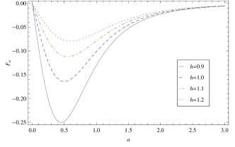
Figure 1: The Casimir force on the $x$ direction vs.$a$ in $D=3$ dimension for different $h$. The Casimir force decreases with $h$ increasing and the maximum value of the force magnitude $\frac{2\pi^{2}}{45h^{5}}\sqrt{\frac{5^{5}}{6^{6}}}$ appears at $a=\frac{h}{\sqrt{5}}$.

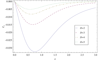
Figure 2: The Casimir force on the $x$ direction vs.$a$ in different dimensions. Here we take $h=1.5$. It is clearly seen that the Casimir force decreases with $D$ increasing, and the value of $a$ where the maximum value of the force is achieved also gets smaller with $D$ increasing.

IV Massive scalar field

In this section, we extend our discussion to the case of massive scalar field. A scalar field $\phi$ defined in the $(D+1)$-dimensional flat spacetime satisfies the equation as follows

$$\left(\partial_{t}^{2}-\partial_{i}^{2}+\mu^{2}\right)\phi(t,x^{\alpha},x^{T})=0\,,$$ (25)

where $\mu$ is the mass of $\phi$ field. In this case, we have

$$\omega_{n}^{2} = k_{T}^{2}+k_{x}^{2}+\left(-\frac{2\pi n}{h}+\frac{k_{x}}{h}a\right)^{2}+\mu^{2}$$ (26)

$$= k_{T}^{2}+k_{z}^{2}+\left(\frac{2\pi n}{a}+\frac{k_{z}}{a}h\right)^{2}+\mu^{2}\,.$$

where $k_{x}$ and $k_{z}$ satisfy Eq.(10). The Casimir energy density of the massive scalar field in the ($D+1$)-dimensional spacetime is thus given by

$$E_{\mu}^{D} =\frac{1}{2a}\int\frac{d^{D-1}k}{(2\pi)^{D-1}}\sum_{n=-\infty}^{\infty}\sqrt{k_{T}^{2}+k_{z}^{2}+\left(\frac{2\pi n}{a}+\frac{k_{z}}{a}h\right)^{2}+\mu^{2}}\,,$$

To regularize Eq.(27), we use the functional relation

$$\sum_{n=-\infty}^{\infty}\left(bn^{2}+\mu^{2}\right)^{-s}=\frac{\sqrt{\pi}}{\sqrt{b}}\frac{\Gamma\left(s-\frac{1}{2}\right)}{\Gamma(s)}\mu^{1-2s}+\frac{\pi^{s}}{\sqrt{b}}\frac{2}{\Gamma(s)}\sum_{n=-\infty}^{\infty\hskip 5.69046pt\prime}\mu^{\frac{1}{2}-s}\left(\frac{n}{\sqrt{b}}\right)^{s-\frac{1}{2}}K_{\frac{1}{2}-s}\left(2\pi\mu\frac{n}{\sqrt{b}}\right)$$ (28)

where $K_{\nu}(z)$ is the modified Bessel function and the prime means that the term $n=0$ has to be excluded. After tedious deduction, we have

$$E_{R,\mu}^{D}=-\frac{\mu^{D+1}\Gamma\left(-\frac{D+1}{2}\right)}{2^{D+2}\pi^{\frac{D+1}{2}}}-2\left(\frac{\mu}{2\pi\sqrt{a^{2}+h^{2}}}\right)^{\frac{D+1}{2}}\sum_{n=1}^{\infty}n^{-\frac{D+1}{2}}K_{\frac{D+1}{2}}\left(n\mu\sqrt{a^{2}+h^{2}}\right)$$ (29)

For $\nu>0$ and $z\rightarrow 0$, the Bessel function has the asymptotic expression $K_{\nu}(z)\rightarrow\frac{2^{\nu-1}\Gamma(\nu)}{z^{\nu}}$, so it is not difficult to find that when $\mu\rightarrow 0$, the Casimir energy recover the result of the massless case.

Using Eq.(20) and $K_{\nu}^{\prime}(z)=\frac{\nu}{z}K_{\nu}(z)-K_{\nu+1}(z)$ where $K_{\nu}^{\prime}(z)=dK_{\nu}(z)/dz$, we have the Casimir force

$$F_{a,\mu}=-\frac{2\mu a\left((\mu a)^{2}+(\mu h)^{2}\right)^{\frac{D+1}{4}}}{\left(2\pi\right)^{\frac{D+1}{2}}\left(a^{2}+h^{2}\right)^{\frac{D+2}{2}}}\sum_{n=1}^{\infty}n^{-\frac{D-1}{2}}K_{\frac{D+3}{2}}\left(n\mu\sqrt{a^{2}+h^{2}}\right)$$ (30)

We study numerically the behavior of the Casimir force on $x$ direction as a function of $a$ for different $h$ and $D$. We find that the Casimir force is still attractive and it has a maximum value similarly to massless case. For given values of $D$ and $\mu$, the behavior of the force for different $h$ is similar to that in massless case. But for given values of $h$ and $\mu$, the behavior of the force for different $D$ is opposite to that in massless case. The force increases with $D$ increasing and the position of the maximum value move to larger $a$ as $D$ increasing. We plot the force as a function of $a$ in Fig. 3 for $\mu=1,h=1$ and $D=2,3,4,5$ respectively and it is easy to find the difference between Fig. 3 and Fig. 2.

Because the precise way the Casimir force varies as the mass changes is worth studying, we give the rate of massive and massless cases as follows

$$\frac{F_{a,\mu}}{F_{a,0}}=\frac{\left((\mu a)^{2}+(\mu h)^{2}\right)^{\frac{D+3}{4}}}{(D+1)2^{\frac{D-1}{2}}\Gamma\left(\frac{D+1}{2}\right)\zeta(D+1)}\sum_{n=1}^{\infty}n^{-\frac{D-1}{2}}K_{\frac{D+3}{2}}\left(n\mu\sqrt{a^{2}+h^{2}}\right)$$ (31)

In the case of odd-dimensional space, Eq.(31) can be reduced to

$$\frac{F_{a,\mu}}{F_{a,0}}=\frac{2(2j+1)!!\left((\mu a)^{2}+(\mu h)^{2}\right)^{\frac{j+2}{2}}}{\left(2\pi\right)^{2j+2}|B_{2j+2}|}\sum_{n=1}^{\infty}n^{-j}K_{j+2}\left(n\mu\sqrt{a^{2}+h^{2}}\right)$$ (32)

where $j=1,2,...$. Obviously, the ratio tends to 1 when $\mu\rightarrow 0$ and it tends to zero when $\mu\rightarrow\infty$.

Fig.4 is the illustration of the ratio of the Casimir force in massive case to that in massless case varying with the mass in $D=3$ dimension. The curves correspond to $a=1$ and $h=0.1,1,2,3$ respectively. Fig.5 is the illustration of the ratio of the Casimir force in massive case to that in massless case varying with the mass for different dimensions. The curves correspond to $a=1,h=0.1$ and $D=2,3,4,5$ respectively. It is clearly seen from the two figures that the Casimir force decreases with $\mu$ increasing, and it approaches zero when $\mu$ tends to infinity. The plots also tell us the Casimir force for a massive field decreases with $h$ increasing but it increases with $D$ increasing. For the latter, the behavior of the Casimir force in massive case is different from that of massless case.

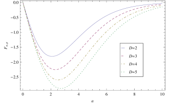
Figure 3: The Casimir force on the $x$ direction vs.$a$ in different dimensions for a massive scalar field. Here we take $h=1,\mu=1$ and $D=2,3,4,5$ respectively. It is clearly seen that the Casimir force increases with $D$ increasing, and the maximum value of the force moves to larger $a$ as as $D$ increasing, which is a feature that opposite to massless case.

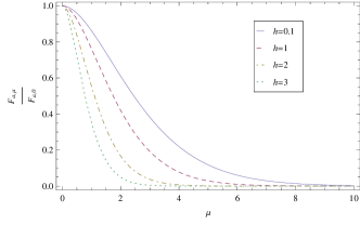
Figure 4: the ratio of the Casimir force in massive case to that in massless case varying with the mass for different $h$ in $D=3$ dimension. The curves correspond to $a=1$ and $h=0.1,1,2,3$ respectively.

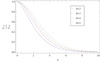
Figure 5: the ratio of the Casimir force in massive case to that in massless case varying with the mass for different dimensions. We take $a=1$ and $h=0.1$.

V Conclusion

In this paper, the quantum spring is investigated in $(D+1)$-dimensional spacetime by using the zeta function techniques for both massless and massive scalar field, and in conclusion, we summarize our results as the following

• For the massless scalar field, the exact expressions of the Casimir energy and Casimir force are obtained in arbitrary $D+1$ dimensional spacetime, and when $D$ is odd, the energy and force could be expressed in terms of the Bernoulli numbers, but for even values of $D$, they can only be expressed in terms of the Riemann $\zeta$ function.

• For the massive scalar field, we also get the exact results of the Casimir energy and force. To see the effect of the mass, we compare the results with that of the massless one and we found that the Casimir force approaches the result of the force in the massless case when the mass tends to zero and vanishes when the mass tends to infinity.

• For both massless and massive scalar field, the Casimir force in $x$ direction decreases when $h$ is increasing and there is a symmetry of $a\leftrightarrow h$ for the Casimir energy. The Casimir force has a maximum value, and the critical value of $a$ to get this maximum value increases with $h$ increasing in both cases.

• There is a little different behavior of the Casimir force for the massless and massive field. That is the Casimir force and its maximum critical value of $a$ decrease with $D$ increasing in the massless case, but increase with $D$ increasing in the massive case.

As is known that the Casimir effect can apply to the cosmology with extra dimensions, the effect of the quantum spring in the (1+3+2)- dimensional cosmology is worth considering and we will study it in our further workZhai2 .