Abstract

The locomotion of Caenorhabditis elegans exhibits complex patterns. In particular, the worm combines mildly curved runs and sharp turns to steer its course. Both runs and sharp turns of various types are important components of taxis behavior. The statistics of sharp turns have been intensively studied. However, there have been few studies on runs, except for those on klinotaxis (also called weathervane mechanism), in which the worm gradually curves toward the direction with a high concentration of chemicals; this phenomenon was discovered recently. We analyzed the data of runs by excluding sharp turns. We show that the curving rate obeys long-tail distributions, which implies that large curving rates are relatively frequent. This result holds true for locomotion in environments both with and without a gradient of NaCl concentration; it is independent of klinotaxis. We propose a phenomenological computational model on the basis of a random walk with multiplicative noise. The assumption of multiplicative noise posits that the fluctuation of the force is proportional to the force exerted. The model reproduces the long-tail property present in the experimental data.

Keywords: nematode, random walk, multiplicative noise, power law, chemotaxis

INTRODUCTION

The soil nematode Caenorhabditis elegans (C. elegans) is unique in that its 302 neurons and their network have been fully identified [1]. In addition, the entire genomic sequence of C. elegans has been determined [2]. On agar surfaces, the worm lies on one of its two sides and exhibits complex locomotion by crawling forward and backward. Complex locomotion is particularly evident when the worm responds to various types of sensory inputs. Examples of such functional responses include chemotaxis, thermotaxis, and isothermal tracking. The identification of specific neurons involved in these and other responses has been a topic of intensive research [3, 4, 5, 6, 7].

The complex locomotion of C. elegans, which underlies functional responses of the worm, accompanies undulations of the entire body with a period of 2–3 s. In general, trajectories of the worm are not straight but mildly curved. The worm often turns sharply. Sharp turning events are called under different names, such as reversals, sharp turns, and omega turns, depending on the specific manner of turning. A bout of these sharp turning events is generally called a pirouette, and pirouette is known to improve the efficiency of the worm’s locomotion toward chemoattractants (chemotaxis) [8]. Computational modeling has been a useful tool for understanding the locomotion. Most existing computational models assume that sharp turning events, or pirouettes, are the main drive of the functional locomotion behavior of the worm [8, 9, 10, 11].

Recently, another mechanism of chemotaxis was discovered [7]. It was called weathervane mechanism in [7], but more generally called klinotaxis [12]. In klinotaxis in C. elegans, an animal performing a run (segment of trajectory between adjacent sharp turns; see MATERIALS AND METHODS for definition) senses the spatial gradient of chemical compounds in the direction lateral to its forward movements and gradually curves toward a higher concentration of the chemicals. This is distinct from the pirouette mechanism in which pirouettes occur frequently when the concentration of the attractant progressively decreases [8], which is a form of klinokinesis [12]. Klinotaxis suggests that modeling the trajectory of the worm by the combination of pirouettes and straight runs, which do not allow for klinotaxis, may be an oversimplification. There have been few computational studies of runs, except for some on klinotaxis [7] and isothermal tracking [13].

In this paper, we analyze run data of the locomotion of C. elegans in either the absence or presence of a chemoattractant in detail. Our main finding is that the curving angle per unit time exhibits a long-tail distribution (the precise definition of the curving angle is given in MATERIALS AND METHODS). This finding is robust against the influence of the attractant, laser ablation of neurons, and bias in the curving inherent in each worm. Then, we propose a minimal computational model using a correlated random walk, which has been used for modeling the migration of insects and mammals [14, 15, 16, 17, 18]. In contrast to these previous cases, the increment of the curving angle cannot be modeled as a Gaussian distribution, which would arise as a summation of many independent and identically distributed noisy microscopic movements [19, 20]. A random walk with multiplicative random noise [21] explains the long-tail behavior in the locomotion of C. elegans.

MATERIALS AND METHODS

Experimental details

We analyzed a subset of the experimental data used in ref. [7]. We briefly explain the experimental setup and the data (see ref. [7] for details).

We used data from two sets of experiments. In one environment, each worm was placed on an agar plate without NaCl. This data set is the main focus of the present study. Data obtained from 46 worms in this environment were analyzed. In the other environment, we placed the worms on a grid format plate in which NaCl was spotted in a grid pattern and allowed to diffuse on chemotaxis agar as follows. Data obtained from 53 worms in this environment were analyzed.

Worms (C. elegans; Bristol strain N2) were cultured at 20^∘C using a standard technique. The agar plates contained 10 ml of 1 mM CaCl₂, 1 mM MgSO₄, 5 mM potassium phosphate, pH 6.0, and 2% agar in a 9-cm-diameter plastic dish. For assays with NaCl (chemotaxis assays), the agar plates were prepared as follows: 1 $\mu$M each of 200 mM NaCl in a low-salt buffer was spotted onto 12 points in a grid, which were spaced 2 cm apart; the positions of the centers of the spots were $(x,y)$ = (10 mm, 10 mm), (10 mm, $-$10 mm), ($-$10 mm, 10 mm), and so on (see [7]). The assay plates were left for 1 h after spotting the NaCl-containing buffer.

In the tracking system, images were captured and analyzed to locate the centroid of the worm. Images were captured at intervals 0.4–0.6 s. Each worm was tracked for 20 min after being placed on the agar plate. Tracking data were discarded when a worm was considered to be immobile during an entire recording session.

Data analysis

A sample trajectory of a worm in the two-dimensional plane is shown in Fig. 1A. The symbols represent the location at each image capture. We discard sharp turns (gray squares) defined in the following and analyze the rest of the data (dark circles). To this end, we define the displacement vector as the difference between the coordinate observed at a time point and that observed at the previous time point (Fig. 1B). The angle from the $x$-axis to the displacement vector at time $t_{i}$ measured clockwise is denoted as $\theta_{i}$. Following [8], we define the curving rate as

$$\phi_{i}=\frac{\theta_{i}-\theta_{i-1}}{t_{i}-t_{i-1}}.$$ (1)

This definition is slightly different from that in [7], in which the curving rate is defined by the derivative of $\theta$ with respect to the distance traveled. The determination of a curving rate involves three successive data points. The speed in addition to the curving rate is required to specify the locomotion of the worm. Although the speed of the worm varies with time, we neglect these variations, as in the case of previous modeling studies [8, 7, 22]

We remove sharp turns as follows (Fig. 1C). A sharp turn is defined as an event in which $|\theta_{i+1}-\theta_{i}|>100^{\circ}$ is satisfied. A sharp turn segment (shaded area in Fig. 1C) is defined as the segment of the trajectory within 0.1 mm from a sharp turn event. The length of the trajectory is measured by the accumulated length of the piecewise linear path connecting the two-dimensional coordinates. We remove all the sharp turn segments and analyze the rest of the data, which we call the run data. A run is a section of the trajectory between two successive sharp turn segments. A single worm generates a trajectory that generally includes multiple runs.

Our data were recorded at irregular intervals. To avoid the technical complication of calculating the autocorrelation of the curving rate in this situation, we proceed as follows. We first generate a continuous trajectory on the two-dimensional plate from a sequence of the coordinates of the worm by using the third spline interpolation (numerically implemented using GNU Scientific Library). Then, we resample discrete time series of the coordinates from the interpolated continuous trajectory every 0.3 s. Next, we detect sharp turns of the resampled trajectory and exclude the sharp turn segments. $\phi_{s,i,j}$, $\ell_{s,i}$, and $M_{s}$ denote the $j$th curving rate in the $i$th run of the $s$th worm ($1\leq s\leq 46$), length of the $i$th run of the $s$th worm, and number of runs of the $s$th worm, respectively. We combine all the runs from all the worms to calculate a single autocorrelation function because reliably calculating the autocorrelation necessitates many data points.

The number of data points used for calculating the autocorrelation function with lag $\tau$ is given by

$$L_{\tau}=\sum_{s=1}^{46}\sum_{i=1}^{M_{s}}\max(\ell_{s,i}-\tau,0).$$ (2)

The average curving rate for the data points that are included in the calculation of the two-point correlation function with lag $\tau$ is equal to

$$\left<\phi\right>_{\tau}\equiv\frac{1}{L_{\tau}}\sum_{s=1}^{46}\sum_{i=1}^{M_{s}}\sum_{j=1}^{\max(\ell_{s,i}-\tau,0)}\phi_{s,i,j}.$$ (3)

The autocorrelation function with lag $\tau$ (i.e., $0.3\times\tau$ s), denoted by $R_{\tau}$, is defined by

$$R_{\tau}=\frac{\displaystyle{\frac{1}{L_{\tau}}\sum_{s=1}^{46}\sum_{i=1}^{M_{s}}\sum_{j=1}^{\max(\ell_{s,i}-\tau,0)}\left(\phi_{s,i,j}-\left<\phi\right>_{\tau}\right)\left(\phi_{s,i,j+\tau}-\left<\phi\right>_{\tau}\right)}}{\displaystyle{\sqrt{\frac{1}{L_{\tau}}\sum_{s=1}^{46}\sum_{i=1}^{M_{s}}\sum_{j=1}^{\max(\ell_{s,i}-\tau,0)}\left(\phi_{s,i,j}-\left<\phi\right>_{\tau}\right)^{2}}{\sqrt{\frac{1}{L_{\tau}}\sum_{s=1}^{46}\sum_{i=1}^{M_{s}}\sum_{j=1}^{\max(\ell_{s,i}-\tau,0)}\left(\phi_{s,i,j+\tau}-\left<\phi\right>_{\tau}\right)^{2}}}}}.$$ (4)

Note that $R_{0}=1$. We verified that the interpolation does not significantly affect the trajectory or the distributions of $\phi$. We employed the spline interpolation only for calculating the autocorrelation function.

When NaCl is present, the concentration of NaCl created by a single spot of NaCl was evaluated by the solution of the diffusion equation: $N_{0}\exp(-r^{2}/(4Dt))/(4\pi dDt)$, where $N_{0}=2.0\times 10^{-4}$ (mM) is the amount of NaCl spotted, $D=1.5\times 10^{-3}$ (mm²/s) is the diffusion constant of NaCl, $d=1.8$ (mm) is the thickness of the plate, $t$ is the time (in seconds) after spotting, and $r$ is the distance (in millimeters) from the spot. The summation of the estimated NaCl concentration based on 12 NaCl spots defines the total concentration of NaCl, which we denote by $C$.

To examine klinotaxis, we compute the gradient of the concentration of NaCl along two directions. One is the forward direction, which is parallel to the displacement vector. The corresponding gradient is denoted by $\mathrm{d}C/\mathrm{d}x_{\mathrm{f}}$. The other is the lateral direction, which is perpendicular to the forward direction. The corresponding gradient is denoted by $\mathrm{d}C/\mathrm{d}x_{\mathrm{\ell}}$. We define $\mathrm{d}C/\mathrm{d}x_{\mathrm{\ell}}$ to be positive if $C$ on the right side of the worm, when viewed from above, is larger than that on the left side.

RESULTS

Long-tail behavior of curving rate

We analyze runs from two sets of experiments from different environments: ones with and without a gradient of the NaCl concentration (NaCl gradient for short). We mainly focus on the data recorded in the absence of an NaCl gradient.

A time series of the curving rate $\phi$ of a worm during a run is shown in Fig. 2A. $\phi$ has a periodic component and accompanies large fluctuations. Periodic behavior with a period of approximately 3 s is derived from the body undulation. The autocorrelation function of the curving rate shown in Fig. 2B indicates oscillatory damping.

The distribution of $\phi$ for a typical worm is indicated by the dashed line in Fig. 2C. The distribution has two peaks owing to the oscillatory undulation. The significance of the two peaks varies between worms and runs. When we combine the data of all the worms, the distribution of $\phi$ is unimodal (solid line in Fig. 2C), which reflects the heterogeneity of the worms. To inspect the tails of the distribution, we divide the samples into a group with $\phi>0$ and that with $\phi<0$. For a single worm, the cumulative distributions of $|\phi|$, defined in the present study as the fraction of samples among all the samples such that the absolute value is larger than $|\phi|$, are separately shown for the two groups in Fig. 2D. Remarkably, both two cumulative distributions of $\phi$ have long tails. The long tails are also evident when we combine the data of all the worms (Fig. 2D). The mean of $\phi$ for the combined data is almost equal to zero, and the standard deviation of $\phi$ is equal to $15.8$. The cumulative distribution of the Gaussian distribution with mean zero and standard deviation 15.8 is indicated by the dot-dashed line in Fig. 2D. The distribution of $\phi$ is not accurately fitted by the Gaussian distribution because of the long tail present in the experimental data. A manual power-law fit to the tail of the cumulative distribution of $|\phi|$ yields the power law $\propto|\phi|^{-2.5}$ (i.e., $\propto|\phi|^{-3.5}$ for the original distribution). The exponent and the significance of the power law depend on the worm and on the sign of $\phi$. Nevertheless, for all the data examined, the tail is much longer than that of the Gaussian distribution of the same value of the standard deviation.

To show that the observed long-tail distribution of $\phi$ is not a byproduct, we perform a few tests. First, the long tail is not caused by sharp turns. If we include the sharp turns in the analysis, we find a peak at a large value of $\phi$ (Fig. 2E) that is distinct from the long tail observed in the run data. For visibility, the original distributions of $|\phi|$, not the cumulative ones as in other similar figures, are plotted in Fig. 2E.

Second, the long tail is not caused by the immobility of the worm. The mean of $|\phi|$ is plotted against the instantaneous speed of the worm in Fig. 3A. $|\phi|$ tends to be large when the worm runs slowly. Excluding the values of $\phi$ for which the instantaneous speed of the worm is small, i.e., less than 0.05 mm/s, preserves the long-tail distribution (Fig. 3B).

Third, the occurrence of a large value of $|\phi|$ is not restricted to periods near sharp turns. We recover the long-tail distribution even if we exclude a significant length of run (i.e., 6 s) before and after sharp turns (Fig. 3C).

In the presence of an NaCl gradient, the run is chiefly characterized by klinotaxis [7], according to which the worm senses the lateral gradient of NaCl and gradually curves toward the direction in which the NaCl concentration increases. We quantified klinotaxis by following the methods developed in [7]. In Fig. 4A, the mean of $\phi$ of single worms is plotted against the values of the lateral and forward gradients of NaCl concentration. The error bars in the figure represent the standard deviations calculated based on the mean values of $\phi$ from different worms. Klinotaxis is evident from the positive correlation between $\phi$ and the lateral NaCl gradient (i.e., $\mathrm{d}C/\mathrm{d}x_{\mathrm{\ell}}$). During the run, the worm tends to curve its body to encounter a higher concentration of the NaCl. Note that $\phi$ and the forward NaCl gradient (i.e., $\mathrm{d}C/\mathrm{d}x_{\mathrm{f}}$) are almost uncorrelated.

Figures 4B and C indicate that the standard deviation and the skewness of $\phi$ for single worms are insensitive to both the lateral and forward NaCl gradients. The dependence of the skewness on the NaCl gradient (Fig. 4C), which was found previously [7], does exist but is negligible in the present analysis. Therefore, we expect that the NaCl gradient effectively shifts the distribution of $\phi$ by an amount proportional to the lateral NaCl gradient but hardly changes the shape of the distribution of $\phi$. Sample distributions of $\phi$ conditioned by two ranges of $\mathrm{d}C/\mathrm{d}x_{\mathrm{\ell}}$ values are compared in Fig. 4D. They do not differ considerably except for translation, as expected.

Figure 4 suggests that klinotaxis translates the distribution of $\phi$ by a small amount and does not affect the long tails. A sample trajectory and the distributions of $\phi$ obtained from the experiments in the presence of an NaCl gradient are shown in Fig. 5. The results are qualitatively similar to those obtained from the experiments in the absence of an NaCl gradient (Fig. 2).

We conclude that the long-tail behavior of the run is robustly observed both in the absence and presence of an NaCl gradient.

Computational modeling

We developed a phenomenological model of the run on the basis of the correlated random walk [8, 23, 14, 19, 15, 16, 20, 17, 18, 7].

We indexed the discrete time by $i$, i.e., $t_{i}=t_{i-1}+\Delta t$, where $\Delta t$ is a time interval. We modeled the reorientation of the worm at time $t_{i}$ by

$$\phi_{i}=R\cos\left(\eta_{i}\right)+\tilde{\xi}_{i},$$ (5)

$$\eta_{i}=\eta_{i-1}+\frac{2\pi}{T_{i}}\left(t_{i}-t_{i-1}\right),$$ (6)

where $R$, $\eta_{i}$, and $T_{i}$ are the amplitude, phase, and instantaneous period of undulation, respectively. $\tilde{\xi}_{i}$ is the noise inherent at time $t_{i}$.

If $\tilde{\xi}_{i}$ were independent Gaussian noise, as is the case for the standard correlated random walk, the long-tail behavior of the curving rate is not reproduced. Therefore, we assumed multiplicative noise $\tilde{\xi}_{i}$ [21], such that

$$\tilde{\xi}_{i}=\xi_{i}\phi_{i-1},$$ (7)

where $\xi_{i}\in\mathcal{N}(0.0,\sigma)$; $\xi_{i}$ is chosen from the normal distribution with mean 0 and standard deviation $\sigma$. The procedure for fitting the parameter values is described in Appendix I.

The assumption of random multiplicative noise is based on the premise that a large movement accompanies a proportionally large noise, which is known for the arm and hand movements of humans [24, 25, 26, 27]. To examine the plausibility of this assumption, we consider an alternative model in which long-tail noise is directly applied in each time step. If $\tilde{\xi}_{i}$ in Eq. 5 is the independent long-tail noise, the long-tail distribution of $\phi_{i}$ is produced. By allowing an autoregressive (AR) term with which to calibrate the autocorrelation of $\phi_{i}$, we define the alternative model by replacing Eq. 5 by $\phi_{i}=R\cos\left(\eta_{i}\right)+w\phi_{i-1}+\tilde{\xi}_{i}$, where $0\leq w<1$. Note that $\tilde{\xi}_{i}$ is a long-tail noise; the AR model with the Gaussian $\tilde{\xi}_{i}$, as is usually assumed, does not yield the long-tail distribution of $\phi_{i}$ irrespective of the parameter values and the number of autoregressive terms on the right-hand side of the model. We compare the two models by measuring $\left<\left(\phi_{i}-w\phi_{i-1}\right)^{2}\right>$, where $\left<\cdot\right>$ is the average over $i$ for a given $|\phi_{i-1}|$. For the alternative long-tail noise model, we obtain $\left<\left(\phi_{i}-w\phi_{i-1}\right)^{2}\right>=\left<\left(R\cos\left(\eta_{i}\right)+\tilde{\xi}_{i}\right)^{2}\right>$. $\tilde{\xi}_{i}$ is identically distributed, and its typical magnitude is much larger than that of the sinusoidal undulation (i.e., $R\cos(\eta_{i})$) under the fitted parameter values. Therefore, $\left<\left(\phi_{i}-w\phi_{i-1}\right)^{2}\right>\approx\left<\tilde{\xi}_{i}^{2}\right>$ would depend little on $|\phi_{i-1}|$ and serve as an estimate of the magnitude of the noise for a proper value of $w$. In contrast, for our multiplicative noise model, Eqs. 5 and 7 imply that $\left<\left(\phi_{i}-w\phi_{i-1}\right)^{2}\right>$ increases with $|\phi_{i-1}|$.

It turns out for any $w$ that $\left<\left(\phi_{i}-w\phi_{i-1}\right)^{2}\right>$ and $|\phi_{i-1}|$ are positively correlated for both the experimental data (Fig. 6A) and the multiplicative noise model (Fig. 6B). This is not the case for the long-tail noise model with $w=0.95$ (Fig. 6B) or any other values of $w$; the plots for other values of $w$ almost completely overlap with those for $w=0.95$ shown in Fig. 6B. Therefore, at least some components of the locomotion are likely to be explained by the multiplicative noise. We have verified that the addition of the AR terms to the multiplicative noise model little affects the behavior of the model except for some changes in the autocorrelation of $\phi_{i}$.

A sample trajectory obtained from the numerical simulations of the multiplicative noise model is shown in Fig. 7A, which is qualitatively similar to that shown in Fig. 2A. In Fig. 7B, the autocorrelation function obtained from the model (dashed line labeled “constant $T_{i}$”) is compared with that of the experimental data (solid line). Even though the model reproduces the oscillatory nature of the autocorrelation function, the autocorrelation does not decay, indicating the excessive periodicity inherent in the model. The strong periodicity results from the fact that the undulation period $T_{i}$ is fixed. The distribution of $\phi$ and its long tail obtained from the numerical simulations roughly resemble those of the experimental data (Fig. 7C and D).

The undulation period of the experimental data fluctuates. To incorporate this factor, we extended the model by allowing $T_{i}$ to fluctuate with time. We set $T_{i}=2.8+\zeta$, where $\zeta\in\mathcal{N}(0.0,0.9)$. We generated $T_{i}$ until a positive value of $T_{i}$ was obtained. This modification of the model yielded the exponential decay in the autocorrelation function, as found in the experimental data (dash-dotted line labeled “fluctuating $T_{i}$” in Fig. 7B). The modified model does not quantitatively agree with the autocorrelation function of the experimental data, partly because the fluctuation in $T_{i}$ is crudely implemented. Note that the modification of the model does not change the distribution of $\phi$ (dash-dotted lines in Figs. 7C and D). The sample trajectory is also similar to that of the original model and that of the experimental data.

The long-tail behavior is not restricted to the specificity of the multiplicative noise, as defined by Eq. 7. The behavior of the model is almost the same when we replaced Eq. 7 with a different noise model given by $\tilde{\xi}_{i}=\xi_{i}(\phi_{i-1}+\phi_{i-2})/2$ (Fig. 8).

Under NaCl gradients, klinotaxis seems to simply translate the distribution of $\phi$ (Fig. 4). Therefore, we extended the model such that klinotaxis adds linearly to the random walk. In other words, the curving rate observed under NaCl gradients is assumed to be the summation of $\phi_{i}$ given by Eq. 5 and the klinotaxis term $\alpha\times\mathrm{d}C/\mathrm{d}x_{\mathrm{\ell}}$. In the numerical simulations, we set $\alpha=19.24$, which is the value of the slope determined by the linear regression for the mean of the data shown in Fig. 4A.

The numerical results in the presence of an NaCl gradient almost overlap those from the computational model in the absence of an NaCl gradient shown in Fig. 7. This implies that the model reproduces the long-tail behavior of $\phi$, as observed in the experimental data in the presence of an NaCl gradient (Fig. 5). We did not calculate the autocorrelation function because the curving rate is nonstationary when the worm performs chemotaxis. We have verified that our model worm performs chemotaxis as in previous models and experimental data [8, 7].

DISCUSSION

We have analyzed the runs of C. elegans and discovered long-tail distributions of the curving rate. We have proposed a phenomenological model that qualitatively reproduces the behavior of the curving rate. Our model is a type of correlated random walk with multiplicative noise.

The long-tail behavior is robust against various types of perturbations. First, it is observed both in the absence and the presence of NaCl gradients such that it is independent of klinotaxis. Second, our results are not restricted to the specific version of the multiplicative noise model assumed in this study (see Fig. 8). Third, the long-tail behavior is robust against laser ablation of various neurons. As shown in Fig. 9, the long-tail behavior is preserved regardless of whether the ablated neurons are responsible for klinotaxis for NaCl chemotaxis (AIZ neurons; see [7]) or not (RIA neurons). This result gives another support to the observation that the long-tail behavior is independent of klinotaxis. We speculate that the long-tail behavior reflects intrinsic properties of the neural circuit for head oscillation, which is currently unidentified. Fourth, the bias in the curving rate that each worm owns [8, 7], perhaps because the worm crawls on one of its sides, does not affect the long-tail behavior (see Appendix II). We have also verified by numerical simulations that the long-tail behavior of $\phi$ does not hamper klinotaxis.

The travel length per unit time obeys the Lévy distribution (i.e., a power-law distribution) for various animals. Such a Lévy flight is suggested to enhance the efficiency of foraging [28, 29]. The long-tail distributions in the curving rate that we have discovered are not directly related to the Lévy flight. In the Lévy flight, the distance of the movement per unit time follows a long-tail distribution. Accordingly, long jumps occasionally occur to possibly accelerate the foraging. In the locomotion of C. elegans, the distance of the movement per unit time is narrowly distributed, which reflects the fact that the worm moves only by means of regular undulation of the body. A long-tail distribution of the curving rate does not appear to affect the long-term locomotion behavior relevant in foraging or taxis.

The trajectories of the worms are highly noisy. The correlated random walk is a useful tool for modeling noisy migrations of C. elegans [8, 23, 7] and other animals [19, 15, 16, 20, 18]. The noise per unit time is often modeled as Gaussian noise [19, 7]. However, Gaussian noise does not lead to distributions with long tails. Obviously, we could reproduce the long tail if independent noise obeying the long-tail distribution is applied at each time step [17]. However, this independent-noise model contradicts the positive correlation between the statistics of the consecutive curving rates present in the data (Fig. 6). To be consistent with both the long-tail behavior and the positive correlation, we have assumed that the amplitude of the noise is proportional to the curving rate. This assumption is based on the premise that exerting a large force accompanies a proportionally large noise. This is the case in the motor activities of human beings; the amplitude of the physiological noise is proportional to the magnitude of the hand and arm movements or the generated force [24, 25, 26, 27]. We note that the positive correlation in the data is not as strong as the expectation from a random walk with purely multiplicative noise. The locomotion of the actual worm may be generated by combination of multiplicative noise and independent noise. To the best of our knowledge, the relationship between the magnitude of the force and that of the noise has not been analyzed for animals other than humans. An investigation of this issue may be an interesting future problem. Explicit modeling of the animal’s movement should also be attempted in the future.

Appendix I: Determination of parameter values of the computational model

We determined the four fitting parameters of the model, i.e., $\Delta t$, $R$, $T_{i}$, and $\sigma$, as follows. On the basis of the long-term oscillatory period of the data, we set $T_{i}=2.8$ s independent of $i$ (also see Fig. 2A). We also investigated the case of fluctuating $T_{i}$ in the main text. The amplitude of the oscillatory head movement is set to $R=10.0$^∘/s so that the dual peaks in Fig. 2C are roughly recovered. These two parameters are necessary for reproducing the undulation of the worm. The standard deviation of the intrinsic noise (i.e., $\sigma$) controls the dispersion of $\phi$. In order to match the standard deviation of the distribution of $\phi$ with the experimental one, we set $\sigma=0.9$. The parameters $R$ and $\sigma$ mainly control the distribution of $\phi$ for small $|\phi|$ and large $|\phi|$, respectively. It was found that $\sigma$ does not affect the timescale of the autocorrelation to a great extent. $\Delta t$ is a relevant parameter of the present model and mainly affects the timescale of the decay of the autocorrelation function of $\phi$ for small time lags (see Fig. 10). To fit the experimental data in this aspect, we set $\Delta t=0.6$ s.

Appendix II: Worm-dependent bias in curving rate

The standard deviation of $\phi$ in the absence of an NaCl gradient is plotted against the mean of $\phi$ in Fig. 11. One data point corresponds to one worm. Figure 11 indicates that the bias (i.e., mean $\phi$) inherent in each worm is small relative to its standard deviation. However, the effect of this bias is sufficiently large to generate a visible rotating trend of the locomotion.

To examine the effect of the bias on our main results, we considered the curving rate generated by adding a constant bias as well as the klinotaxis term $\alpha\times\mathrm{d}C/\mathrm{d}x_{\mathrm{\ell}}$ to the right-hand side of Eq. 5 [8, 23]. We confirmed that this modification of the model does not significantly affect the distribution of $\phi$ and the shape of the autocorrelation function, regardless of the magnitude of the constant bias. The bias has a significant effect on a long time scale, but not on a short one. Because our analysis of $\phi$ is concerned with a short time scale, we did not detrend the bias in the analysis of our experimental data in the main text.

Note that the concept of the bias discussed here is different from the tendency that the worm migrates in a specific direction in which the concentration of the attractant increases [18].

FIGURE LEGENDS

Figure 1: (A) Sample trajectory of the worm. (B) Definition of the curving rate $\phi_{i}$. (C) Definition of the sharp turn segment (shaded area).

Figure 2: Results obtained from experiments in the absence of an NaCl gradient. (A) Sample trajectory of $\phi$. (B) Autocorrelation function of $\phi$. (C) Distributions of $\phi$ based on the runs of a single worm and those of all the worms. We use a bin width of 4^∘/s . (D) Cumulative distributions of $|\phi|$ (i.e., fraction of values above $|\phi|$) on the log-log scale. The results for one worm and the combined one for all the worms are shown separately for positive and negative values of $\phi$. The dot-dashed line in (D) indicates the cumulative distribution of the Gaussian distribution with mean zero and standard deviation 15.8. (E) Distribution of $|\phi|$ for the data before and after sharp turns are excluded. The data for all the worms are combined to generate each distribution.

Figure 3: (A) Relationship between the mean of $|\phi|$ and the instantaneous speed of the worms. The mean values are calculated from all the runs of a single worm by categorizing the data into bins of width 0.025 mm/s and taking the average in each bin. Then, the mean values from different worms for the same bin are used for calculating the grand mean and standard deviation. The grand mean and error bar defined by the one standard deviation range are plotted in (A). (B) Cumulative distribution of $|\phi|$ when data points for which the speed of the worms is less than 0.05 mm/s are excluded. (C) Cumulative distributions of $|\phi|$ when the data points within 6 s before or after each sharp turn are excluded. For each figure, the data obtained from all the worms are combined to generate the cumulative distribution.

Figure 4: Klinotaxis. (A) Mean, (B) standard deviation, and (C) skewness of $\phi$ for different values of lateral and forward NaCl gradients. The mean, standard deviation, and skewness for a value of the concentration gradient are calculated from all the runs of a single worm. Then, the values from different worms for the same value of the concentration gradient are used for calculating their mean and standard deviation. The mean values, together with the error bar defined by the one standard deviation range, are plotted in (A)–(C). (D) Distributions of $\phi$ conditioned by two ranges of lateral NaCl gradient $\mathrm{d}C/\mathrm{d}x_{\mathrm{\ell}}$. We combined the data of all the worms to make the two distributions sufficiently smooth.

Figure 5: Results obtained from experiments in the presence of an NaCl gradient. (A) Sample trajectory of $\phi$. (B) Distributions of $\phi$. (C) Cumulative distributions of $|\phi|$. See the caption of Fig. 2 for legends.

Figure 6: Testing the multiplicative noise hypothesis. We plot $\sqrt{\left<\left(\phi_{i}-w\phi_{i-1}\right)^{2}\right>}$ against $|\phi_{i-1}|$ for four values of $w$ for (A) experimental data and (B) random walk model with multiplicative noise. The results for the AR model with $w=0.95$ and the power-law noise distribution with exponent 3 are also shown in (B). Each plotted point represents the square root of the average of $\left(\phi_{i}-w\phi_{i-1}\right)^{2}$ in a bin. Each bin has width 20^∘/s and contains the corresponding values of $|\phi_{i-1}|$ obtained from all the worms.

Figure 7: Results obtained from numerical simulations of the computational model in the absence of an NaCl gradient. (A) Sample trajectory of $\phi$ when $T_{i}$ is constant. (B) Autocorrelation function of $\phi$. (C) Distributions of $\phi$. (D) Cumulative distributions of $|\phi|$ on the log-log scale. In (B), (C), and (D), the experimental data, the numerical results with constant $T_{i}$, and those with fluctuating $T_{i}$ are compared.

Figure 8: Numerical results in the absence of an NaCl gradient when a different noise model is used. Eq. 7 is replaced by $\tilde{\xi}_{i}=\xi_{i}(\phi_{i-1}+\phi_{i-2})/2$ with $\xi_{i}\in\mathcal{N}(0.0,1.24)$. We modified the standard deviation of the noise from that of the original model (Eq. 7) to obtain a reasonable fit to the experimental data. Long-tail distributions of $\phi$ are produced, as shown in D. See the caption of Fig. 7 for legends.

Figure 9: Cumulative distribution of $|\phi|$ for the worms subjected to laser ablation of either of two different neurons (RIA and AIZ). The laser-ablated worms are subjected to an NaCl gradient. Each distribution is generated by combining the data of all the worms. The long-tail behavior of the run is supported by these data. The scaling exponent of the long-tail distribution depends on the type of ablation. The results in the absence of ablation are also plotted for comparison.

Figure 10: Numerical results for different values of $\Delta t$. (A) Cumulative distributions of $|\phi|$. The distribution of the curving rate is nearly independent of the value of $\Delta t$ in the computational model. (B) Autocorrelation function of $\phi$. The autocorrelation function for small time lags depends on $\Delta t$. A small $\Delta t$ yields a rapid decay of the autocorrelation function for a small lag. In the main text, we set $\Delta t=0.6$ s such that the autocorrelation function for small time lags is close to that of the experimental data.

Figure 11: Relationship between the standard deviation of $\phi$ and the mean of $\phi$ for each worm in the absence of an NaCl gradient.

FIGURES

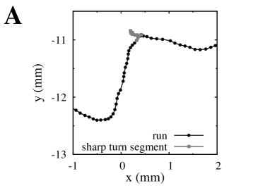
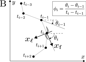
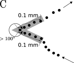
Figure 1:

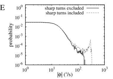
Figure 2:

Figure 3:

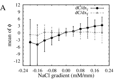
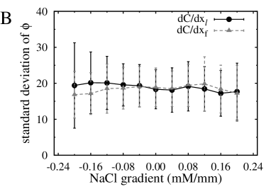
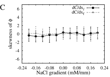
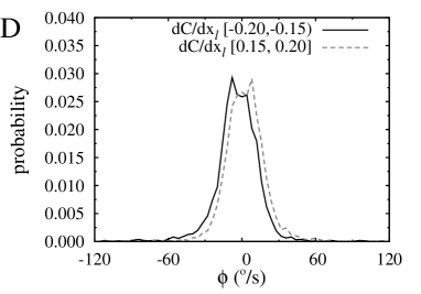
Figure 4:

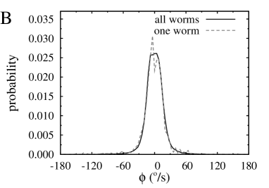
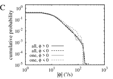
Figure 5:

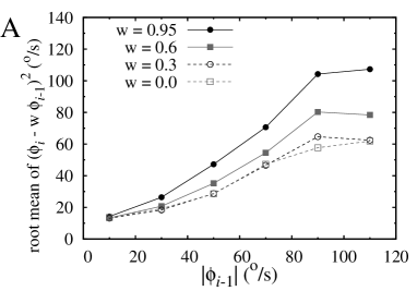
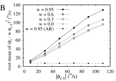
Figure 6:

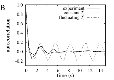
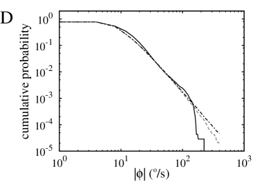
Figure 7:

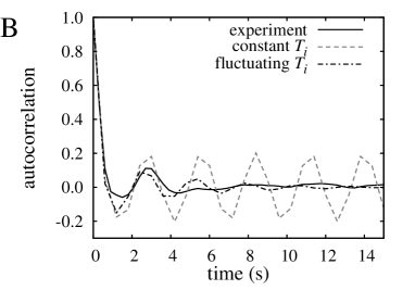
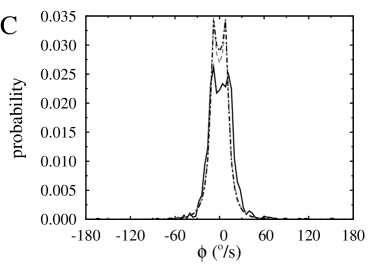
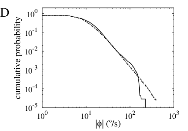
Figure 8:

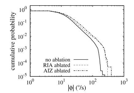
Figure 9:

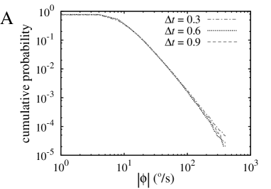
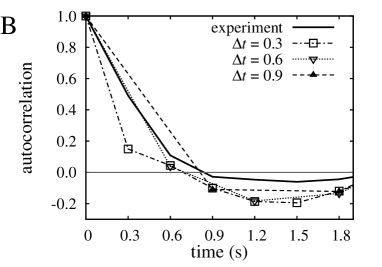
Figure 10:

Figure 11:

References

- [1] J.G. White, E. Southgate, J.N. Thomson, S. Brenner, The structure of the nervous system of Caenorhabditis elegans, Philos. Trans. R. Soc. London B 314 (1986) 1–340.
- [2] The C. elegans Sequencing Consortium, Genome sequence of the nematode C. elegans: a platform for investigating biology, Science 282 (1998) 2012–2018.
- [3] C.I. Bargmann, H.R. Horvitz, Chemosensory neurons with overlapping functions direct chemotaxis to multiple chemicals in C. elegans, Neuron 7 (1991) 729–742.
- [4] C.I. Bargmann, E. Hartwieg, H.R. Horvitz, Odorant-selective genes and neurons mediate olfaction in C. elegans, Cell 74 (1993) 515–527.
- [5] I. Mori, Y. Ohshima, Neural regulation of thermotaxis in Caenorhabditis elegans, Nature 376 (1995) 344–348.
- [6] J.M. Gray, J.J. Hill, C.I. Bargmann, A circuit for navigation in Caenorhabditis elegans, Proc. Natl. Acad. Sci. USA, 102 (2005) 3184–3191.
- [7] Y. Iino, K. Yoshida, Parallel use of two behavioral mechanisms for chemotaxis in Caenorhabditis elegans, J. Neurosci. 29 (2009) 5370–5380.
- [8] J.T. Pierce-Shimomura, T.M. Morse, S.R. Lockery, The fundamental role of pirouettes in Caenorhabditis elegans chemotaxis, J. Neurosci. 19 (1999) 9557–9569.
- [9] T. Matsuoka, S. Gomi, R. Shingai, Simulation of C. elegans thermotactic behavior in a linear thermal gradient using a simple phenomenological motility model, J. Theor. Biol. 250 (2008) 230–243.
- [10] D. Ramot, B.L. MacInnis, H.-C. Lee, M.B. Goodman, Thermotaxis is a robust mechanism for thermoregulation in Caenorhabditis elegans nematodes, J. Neurosci. 28 (2008) 12546–12557.
- [11] K. Nakazato, A. Mochizuki, Steepness of thermal gradient is essential to obtain a unified view of thermotaxis in C. elegans, J. Theor. Biol. 260 (2009) 56–65.
- [12] G.S. Frankel, D.L. Gunn, The orientation of animals, Dover, London, 1961.
- [13] L. Luo, D.A. Clark, D. Biron, L. Mahadevan, A.D.T. Samuel, Sensorimotor control during isothermal tracking in Caenorhabditis elegans, J. Exp. Biol. 209 (2006) 4652–4662.
- [14] D.B. Siniff, C.R. Jessen, A simulation model of animal movement patterns, Adv. Ecol. Res. 6 (1969) 185–219.
- [15] R.L. Hall, Amoeboid movement as a correlated walk, J. Math. Biol. 4 (1977) 327–335.
- [16] P.M. Kareiva, N. Shigesada, Analyzing insect movement as a correlated random walk, Oecologia 56 (1983) 234–238.
- [17] F. Bartumeus, M.G.E. da Luz, G.M. Viswanathan, J. Catalan, Animal search strategies: a quantitative random-walk analysis, Ecology 86 (2005) 3078–3087.
- [18] E.A. Codling, M.J. Plank, S. Benhamou, Random walk models in biology, J. R. Soc. Interface 5 (2008) 813–834.
- [19] R. Kitching, A simple simulation model of dispersal of animals among units of discrete habitats, Oecologia 7 (1971) 95–116.
- [20] P. Bovet, S. Benhamou, Spatial analysis of animal’s movements using a correlated random walk model, J. Theor. Biol. 131 (1988) 419–433.
- [21] H. Takayasu, A.-H. Sato, M. Takayasu, Stable infinite variance fluctuations in randomly amplified Langevin systems, Phys. Rev. Lett. 79 (1997) 966-969.
- [22] N.A. Dunn, S.R. Lockery, J.T. Pierce-Shimomura, J.S. Conery, A neural network model of chemotaxis predicts functions of synaptic connections in the nematode Caenorhabditis elegans, J. Comp. Neurosci. 17 (2004) 137-147.
- [23] J.T. Pierce-Shimomura, M. Dores, S.R. Lockery, Analysis of the effects of turning bias on chemotaxis in C. elegans, J. Exp. Biol. 208 (2005) 4727-4733.
- [24] G.G. Sutton, K. Sykes, The variation of hand tremor with force in healthy subjects, J. Physiol. 191 (1967) 699–711.
- [25] R.A. Schmidt, H. Zelaznik, B. Hawkins, J.S. Frank, J.T. Quinn Jr., Motor-output variability: a theory for the accuracy of rapid motor acts, Psychol. Rev. 86 (1979) 415–451.
- [26] C.M. Harris, D.M. Wolpert, Signal-dependent noise determines motor planning, Nature 394 (1998) 780–784.
- [27] K.E. Jones, A.F. de C. Hamilton, D.M. Wolpert, Sources of signal-dependent noise during isometric force production, J. Neurophysiol. 88 (2002) 1533–1544.
- [28] G.M. Viswanathan, S.V. Buldyrev, S. Havlin, M.G.E. da Luz, E.P. Raposo, H.E. Stanley, Optimizing the success of random searches, Nature 401 (1999) 911–914.
- [29] D.W. Sims, E.J. Southall, N.E. Humphries, G.C. Hays, C.J.A. Bradshaw, et al., Scaling laws of marine predator search behavior, Nature 451 (2008) 1098–1102.