Restricted equilibrium ensembles: Exact equation of state of a model glass

Abstract

We investigate the thermodynamic properties of a toy model of glasses: a hard-core lattice gas with nearest neighbor interaction in one dimension. The time-evolution is Markovian, with nearest-neighbor and next-nearest neighbor hoppings, and the transition rates are assumed to satisfy detailed balance condition, but the system is non-ergodic below a glass temperature. Below this temperature, the system is in restricted thermal equilibrium, where both the number of sectors, and the number of accessible states within a sector grow exponentially with the size of the system. Using partition functions that sum only over dynamically accessible states within a sector, and then taking a quenched average over the sectors, we determine the exact equation of state of this system.

The glassy state is usually considered a non-equilibrium state of matter in the sense that the conventional Boltzmann-Gibbs treatment in terms of partition functions would not work, and yields very different properties of the corresponding “equilibrium state” (e.g. of crystalline quartz, and not of window glass). In this paper, our aim is to develop an equilibrium statistical mechanical description of the glassy state using restricted phase-space ensembles. We consider a system constrained by dynamics to a restricted region of phase space. Within this region, it acts like an equilibrium system. This may be considered as an idealized description for metastable states such as supercooled liquids, or a glass. Focussing on the latter, we note that materials like window glass, for a given history of preparation, and at temperatures sufficiently below the glass temperature, have a well-defined macroscopic density, velocity of sound, and specific heat. Then, over a time scale of microseconds to years, these materials are in some effective restricted thermodynamic equilibrium.

In the restricted equilibrium ensemble corresponding to a glassy state, the partition function sum only extends over a restricted region of the phase space. As an illustrative example of these ensembles, we discuss a simple model. In particular, we determine the exact equation of state (a material -dependent relation between the density, pressure and temperature). To the best of our knowledge, this is the first time the exact equation of state for a model with short -range interactions and showing a glassy phase, is obtained.

The model we study is a lattice gas in one dimension, with a pair potential. The time evolution is assumed Markovian, with detailed balance, but in the glassy regime, the dynamics is non-ergodic, and phase space breaks up into a large number of disconnected sectors. We calculate averages of physical quantities in terms of partition functions within a sector, and then average this over sectors.

The notion of restricted ensembles is not new. Many authors have discussed metastable states in terms of constraints on the regions of phase space available to the system, i.e. phase space is broken into disjoint components, with ergodicity within components[1]. The idea of components, in the context of supercooled liquids and glasses was made more specific as inherent structures by Stillinger and Weber [2]. This gives the energy or free-energy landscape picture, which has been very useful in providing a conceptual framework for the study of glasses. But the actual calculation of the partition function within a component, or the number of components is very difficult, and one usually just postulates the form of the distribution function of these [3]. The study of specific models with Markovian evolution with detailed balance, showing break-down of phase space into disjoint sectors, was pioneered by Fredrickson and Andersen[4], and such kinetically constrained models have been studied a lot recently [5]. However, usually the cases studied have a trivial Hamiltonian, and the main focus is on the relaxational dynamics. Our focus here is on the thermodynamics in the glassy phase.

We should also mention earlier work on metastable states for systems with long-range couplings, as in the Sherrington-Kirkpatrick model of spin-glasses [6], or supercooled liquids [7, 8]. Theories like the mode-coupling theory of glasses mainly discuss the onset of glassiness from the liquid side [9]. An overview of recent work on supercooled liquids and structural glasses may be found in [11, 10].

Our approach uses pico-canonical ensembles, discussed earlier in [12]. The glass transition is built into the system by assuming temperature-dependent rates of local dynamic processes, some of which are set to be exactly zero in the glassy phase. We do not try to describe the approach to the glass transition, but focus on the near-equilibrium behavior away from the glass transition point, in the glassy phase.

1 Definition of the model

The system we study is a hard-core lattice gas on a semi-infinite line of sites, labelled by positive integers $i$, with $i$ varying from $1$ to $\infty$. At each site $i$, there is an occupation number variable $n_{i}$ that takes values $0$ or $1$, depending on whether the site is occupied or not.

There are a total of $N$ particles on the line. On the left, there is an immovable wall at $i=0$. To the right of the rightmost ( the $N$-th) particle, is a movable piston, whose position will be denoted by $L$, and which exerts a constant pressure $p$ on the system. There is an attractive interaction between nearest neighbor occupied sites of strength $J$. For simplicity, we assume that the interaction between piston and particles of the gas, and between the left wall and the particles is the same as that between two particles. Then, with the convention $n_{0}=n_{L}=1$, the Hamiltonian of the system is given by

$$H=-J\sum_{i=0}^{L-1}n_{i}n_{i+1}+pL$$ (1)

We assume that the system evolves by Markovian dynamics, with the following rules:
i) An occupied site with an empty neighbor can exchange position with the neighbor with a rate $\Gamma_{1}\exp(-\beta\Delta E/2)$. Here $\Delta E$ is the difference of energies between the final and initial configurations, and $\beta$ is the inverse temperature. This is represented by the ‘chemical’ equation $01\rightleftharpoons 10$.

ii) An occupied site with two empty neighbors on its left ( or right), can jump two spaces to the left ( right), with a rate $\Gamma_{2}\exp(-\beta\Delta E/2)$. This is represented by the equation $100\rightleftharpoons 001$.

iii) The piston can exchange position with a neighboring empty site. This process is represented by the equation $0P\rightleftharpoons P0$. The corresponding rate is $\Gamma_{3}exp(-\beta\Delta E/2)$.

In our model, the externally controlled variables are the pressure, and temperature. The dynamics conserves the number of particles. Within the model, we are free to prescribe any functional dependence to the rates $\Gamma_{1}$, $\Gamma_{2}$ and $\Gamma_{3}$, and the long-time steady state of the system, and the thermodynamic properties do not depend on the precise values of these parameters. We postulate that $\Gamma_{2}$ and $\Gamma_{3}$ are non-zero for all temperatures, and may be assumed to be independent of temperature and pressure, without any loss of generality. For $\Gamma_{1}(p,T)$, we assume that in two-dimensional control space $(p,T)$, there are regions where it is zero, and in the rest of space, it is not [ fig. 1]. The regions where $\Gamma_{1}(p,T)$ is zero will be called glassy regions.

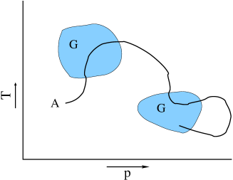
Figure 1: A schematic representation of the glassy and non-glassy regions of the control parameter space $(p,T)$. The non-ergodic glassy regions are shown as shaded regions $G$. $A$ denotes a path in this space, corresponding to particular preparation of the system.

The dynamics of this model is somewhat similar to the model of diffusing reconstituting dimers (DRD model) discussed earlier in [12]. In the DRD model, the only allowed transitions in the low-temperature phase are $110\rightleftharpoons 011$, while in the high temperature phase, $01\leftrightharpoons 10$ is also allowed. These moves are the same as the moves in the present case if the $0$’s and $1$’s are interchanged.

The DRD model was defined in the constant $L$ ensemble, and the right wall could not move. It is not possible to define a satisfactory dynamics of a piston consistent with the dynamics of the DRD model. For example, consider the configuration $1000110011000100P$. Then, it is easily seen that in the DRD dynamics, the piston cannot move to the left of the present position of the rightmost $1$. Hence the DRD lattice gas is incompressible in the non-ergodic phase.

Again, if we move the piston in the DRD model to the right by some macroscopic distance, only dimers can move into the new region. Thus, the long-time steady state is inhomogeneous, and shows a phase separation, with the left region at a higher density than the right, and pressure equilibration between different parts is not possible under the DRD dynamics. This makes the DRD model unsuitable for studying the equation of state. The present model does not suffer from these problems.

2 Sector decomposition and the restricted ensemble

We note that each of the Markov rates here satisfies the detailed balance condition, and the state with the probability of a configuration $C$ is given by the standard Boltzmann -Gibbs weight

$${\rm Prob}(C)=\exp[-\beta H(C)]/{\cal Z}(p,T)$$ (2)

is a steady state. Here ${\cal Z}(p,T)$ is the partition function of the system, given by

$${\cal Z}(p,T)=\sum_{C}\exp[-\beta H(C)]$$ (3)

If $\Gamma_{1}(p,T)$ is non-zero, any configuration of $N$ particles can be reached from any other. Then, the measure given by Eq. (2) is the unique long-time steady state measure.

If however, $\Gamma_{1}(p,T)=0$, then the phase space breaks up into a large number of disconnected parts, called components, or sectors. There are $2^{N}$ disjoint sectors. This is easily seen: Define $x_{i}$ as the position of the $i$-th particle., and $\Delta_{i}=x_{i}-x_{i-1}$. Then the different $\Delta_{i}$ can only change by $\pm 2$. We define $\eta_{i}=\Delta_{i}(mod2)$. Then $\{\eta_{i}\},i=1$ to $N$ are conserved. Note that $\eta_{N+1}$ is not conserved. Clearly, the number of sectors is $2^{N}$. We will denote a sector by ${\mathbb{S}}$, and label these sectors by specifying the $N$ binary integers $\{\eta_{i}\}$.

The conditional probability of a configuration $C$ in the long-time steady state, given that the system is in the sector ${\mathbb{S}}$ is given by

$${\rm Prob}(C|{\mathbb{S}})=\exp[-\beta H(C)]/{\cal Z}_{{\mathbb{S}}}(p,T).$$ (4)

The normalization factor ${\cal Z}_{{\mathbb{S}}}(p,T)$, called the pico-canonical partition function for the sector ${\mathbb{S}}$, is defined as the sum of the standard Boltzmann weights, but only over configurations $C$ that are in the sector ${\mathbb{S}}$,

$${\cal Z}_{{\mathbb{S}}}(p,T)=\sum_{C\in{\mathbb{S}}}\exp[-\beta H(C)]$$ (5)

We consider the control parameters $(p,T)$ being varied slowly along some curve $A$ in the control parameter space (Fig. 1). The curve $A$ may enter and leave the glassy regions several times. When the system is in a non-glassy region, there is a unique equilibrium state of the system, that is independent of the system history, and only depends on the current value of the control parameters. In the glassy regions, the restricted equilibrium state depends on $(p,T)$, and also on the sector. If we vary $(p,T)$, staying within the glassy region, the sector does not change. The relative probabilities of different sectors depend only on the point from which one entered the glassy region.

A precise specification of the sector ${\mathbb{S}}$ requires $N$ bits of information, and if $N$ is large, this is neither possible, nor useful. In an experimental set up, ${\mathbb{S}}$ is specified in some general way in terms of how the system is prepared. We assume that in the beginning, the system is prepared in the ergodic region of the control-parameter space $(p,T)$, and then brought to the desired state by moving along a specified path $A$ adequately slowly. We will specify the macroscopic state of system in a glassy state by the last values of $(p,T)$ in its history, when it was ergodic with $\Gamma_{1}\neq 0$, to be denoted by $(p^{*},T^{*})$. Then, the probability that the system falls in the sector ${\mathbb{S}}$ is given by

$${\rm Prob}({\mathbb{S}})={\cal Z}_{{\mathbb{S}}}(p^{*},T^{*})/{\cal Z}(p^{*},T^{*})$$ (6)

For any observable ${\cal O}$, the long-time average value within the sector ${\mathbb{S}}$ will be denoted by $\langle{\cal O}\rangle_{{\mathbb{S}}}$. This is given by

$$\langle{\cal O}\rangle_{{\mathbb{S}}}=\sum_{C\in{\mathbb{S}}}{\cal O}(C){\rm Prob}(C|{\mathbb{S}})$$ (7)

Often, these can be expressed as appropriate derivatives of the free-energy, as in the standard equilibrium statistical mechanics. For example the average length $\langle L\rangle_{{\mathbb{S}}}$ of the system in the sector ${\mathbb{S}}$ is given by

$$\langle L\rangle_{{\mathbb{S}}}=-k_{B}T\frac{\partial}{\partial p}\log{\cal Z}_{{\mathbb{S}}}(p,T).$$ (8)

The expected value of an observable $\langle{\cal O}\rangle$ in an experiment, for a given history of preparation of the sample, is obtained by further averaging $\langle{\cal O}\rangle_{{\mathbb{S}}}$ over different sectors ${\mathbb{S}}$

$$\langle{\cal O}\rangle=\sum_{{\mathbb{S}}}{\rm Prob}({\mathbb{S}})\langle{\cal O}\rangle_{{\mathbb{S}}},$$ (9)

where ${\rm Prob}({\mathbb{S}})$ is the probability that the system will freeze into the sector ${\mathbb{S}}$, for the given history of preparation.

One can similarly calculate variance of the observable, or the sector-to-sector variation of the sector-mean $\langle{\cal O}\rangle_{{\mathbb{S}}}$. In the simple case we are considering, macroscopic quantities like the mean density can be shown to be self-averaging, and the variance of the sector-means are of ${\cal O}(N)$. The fluctuations, compared to the mean, are smaller by a factor $N^{-1/2}$, for large $N$. If the relative fluctuations are not small for some observable, predicting its value in a particular experimental set-up, without any additional information about the experiment, is clearly not possible. In such cases, one can only determine the probability distribution of such an observable.

In particular, the mean free energy in the glass phase is defined as the free energy, averaged over sectors. We are working in the constant $(p,T)$-ensemble, and the appropriate free energy is the Gibbs free energy $\Phi(p,T)$. The average value of $\Phi(p,T)$ in the glass phase, averaged over sectors, will be denoted by $\langle\Phi_{G}(p,T)\rangle$. This is defined as

$$\langle\Phi_{G}(p,T)\rangle=-k_{B}T\sum_{{\mathbb{S}}}{\rm Prob}({\mathbb{S}})\log{\cal Z}_{{\mathbb{S}}}(p,T)$$ (10)

Note that $\langle\Phi_{G}(p,T)\rangle$ implicitly depends also on $(p^{*},T^{*})$.

3 Equation of state

We now determine the equation of state for this system. Consider first the ergodic case when $\Gamma_{1}\neq 0$. In this case, any allowed configuration can be reached from any other under the Markovian dynamics of the system.

We define $x_{N+1}$ to be the position of the piston $L$. In terms of the variables $\{\Delta_{i}\}$, the Hamiltonian can be written as

$$H=\sum_{i=1}^{N+1}[-J\delta_{\Delta_{i},1}+p\Delta_{i}].$$ (11)

Clearly, in this case, the different $\Delta_{i}$ are independent random variables, we get the partition function of the system ${\cal Z}(\beta,p)$ in the constant temperature and pressure ensemble as [13]

$${\cal Z}(p,T)=w(u,x)^{N+1},$$ (12)

where we have used the notation $u=e^{\beta J}$, and $x=e^{-\beta p}$, and

$$w(u,x)=\sum_{\Delta=1}^{\infty}u^{\delta_{\Delta,1}}x^{\Delta}=ux+\frac{x^{2}}{1-x}.$$ (13)

The mean spacing between the molecules $\langle\Delta\rangle$, which is the inverse of the density of the lattice gas, is given by

$$\langle\Delta\rangle = x\frac{\partial}{\partial x}\log w(u,x)$$ (14)

$$= \frac{x}{w(u,x)}\left[u+\frac{2x-x^{2}}{(1-x)^{2}}\right],{\rm~{}for~{}}\Gamma_{1}\neq 0,~{}$$

and the mean energy per particle $\langle E(u,x)\rangle$ is given by

$$\langle E(u,x)\rangle=-Ju\left[u+\frac{x}{1-x}\right]^{-1},{\rm~{}for~{}}\Gamma_{1}\neq 0.$$ (15)

We can similarly calculate ${\cal Z}_{{\mathbb{S}}}(p,T)$, for any given sector ${\mathbb{S}}$. Define

$$w_{odd}=\sum_{\Delta~{}odd}u^{\delta_{\Delta,1}}x^{\Delta}$$ (16)

and a similar equation for $w_{even}$, where the sum is only over even values of $\Delta$. Then we have

$$w_{odd}=ux+\frac{x^{3}}{1-x^{2}}$$ (17)

and

$$w_{even}=x^{2}/(1-x^{2})$$ (18)

We denote the number of zero $\eta_{i}$’s by $r({\mathbb{S}})$. It is easily seen that

$${\cal Z}_{{\mathbb{S}}}=w_{even}^{r({\mathbb{S}})}w_{odd}^{N-r({\mathbb{S}})}(w_{odd}+w_{even})$$ (19)

Under quenching, $\eta_{i}$ takes the value $0$ with probabilities $w_{even}/w=\alpha^{*}$ independent of $i$, and the value $1$ with probability $1-\alpha^{*}$.

$$\alpha^{*}=\frac{x^{*}}{x^{*}+{x^{*}}^{2}+u^{*}(1-{x^{*}}^{2})}$$ (20)

Then, the probability of a sector ${\mathbb{S}}$ with exactly $j$ odd $\eta_{i}$’s, is given by

$${\rm Prob}({\mathbb{S}})={\alpha^{*}}^{j}{(1-\alpha^{*})}^{N-j}$$ (21)

The variable $r({\mathbb{S}})$ is distributed as a binomial distribution

$${\rm Prob}(r({\mathbb{S}})=j)=^{N}C_{j}~{}{\alpha^{*}}^{j}(1-\alpha^{*})^{N-j}$$ (22)

Thus the distribution of $r({\mathbb{S}})$ is sharply peaked, with maximum at $\alpha^{*}N$, with a width of order ${\cal O}(N^{1/2})$.

A straight forward calculation gives the mean spacing between the particles in the low-temperature phase as

$$\langle\Delta\rangle=x\frac{\partial}{\partial x}[\alpha^{*}\log w_{even}(u,x)+(1-\alpha^{*})\log w_{odd}(u,x)].$$ (23)

Using the expressions for $w_{odd}$ and $w_{even}$ (Eqs. 12 and 13), we finally get

$$\langle\Delta\rangle=(1-\alpha^{*}) \left[1+\frac{2x^{2}(1-x^{2})^{-2}}{u+x^{2}(1-x^{2})^{-1}}\right]+\alpha^{*}\frac{2}{(1-x^{2})},$$ (24)

$${\rm~{}~{}~{}~{}~{}~{}~{}~{}~{}~{}~{}~{}~{}~{}~{}~{}~{}~{}~{}~{}~{}~{}~{}~{}~{}for~{}}\Gamma_{1}=0.$$

This equation, along with Eq. (14)gives the mean volume per particle as a function of $u$ and $x$, and hence is the equation of state of the material. It depends on the history of the system through the parameter $\alpha^{*}$, which depends on onset of the glassy state. From Eq.(22), the sector-to-sector variation of $r({\mathbb{S}})/N$ is of ${\cal O}(N^{-1/2})$, and hence fluctuations in $\langle\Delta\rangle_{{\mathbb{S}}}$ are also small for large systems.

Similarly, we can calculate the mean energy per particle $\langle E(u,x)\rangle$ by taking derivatives with respect to $u$, and we get

$$\langle E(u,x)\rangle=\frac{-Ju(1-\alpha^{*})}{u+x^{2}/(1-x^{2})},{\rm~{}for~{}}\Gamma_{1}=0.~{}~{}$$ (25)

As an example, consider the simple case $J=0$. In this case, there is no energy, and the density is a function of only one variable $\beta p$. In this case, it is easily seen that the equilibrium density is given by

$$\rho_{eq}=1-e^{-\beta p}$$ (26)

.

We assume that the high-density phase is not ergodic, say whenever $\rho>1-x^{*}$. Then, it is easy to see from Eq.(24), that in the non-ergodic phase, the dependence is

$$\rho_{glass}=(1-e^{-2\beta p})\left[2\alpha^{*}+(1-\alpha^{*})(1+e^{-2\beta p})\right]^{-1}$$ (27)

where $\alpha^{*}=x^{*}/(1+x^{*})$.

We have plotted $\rho_{eq}$ and $\rho_{glass}$ in Fig. 2 for $x^{*}=1/2$. We note that the density is continuous at $p=p^{*}$, and the glass is less compressible than the corresponding equilibrium state.

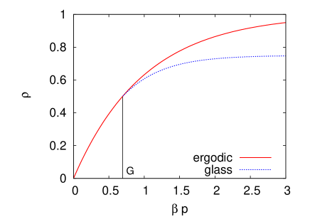
Figure 2: Plot of density $\rho$ as a function of the scaled pressure $\beta p$ for $J=0$, when the regime $\beta p^{*}\geq\log(2)$ is assumed to be non-ergodic. The point of onset of non-erdodicity is denoted by $G$ in the figure.

4 Entropy

The statistical mechanical entropy of a macroscopic system in equilibrium, i.e. one described by the Gibbs ensemble, when the state state is discrete, and the Gibbs ensemble assigns probability $p_{i}$ to the $i$th state, is given by

$$S=-\sum_{i}p_{i}\log p_{i},$$ (28)

This entropy coincides, to leading order in the size of the system, with the thermodynamic entropy of Clausius, and is the same for different ensembles, for ordinary systems ( we are ignoring gravitational interactions). The set of microstates used is always a restricted one, in practice. For example, when considering argon gas below $10^{3}~{}^{\circ}$K, we do not consider the ionized states, or the excited nuclear states. There is some controversy in the glass literature [14] about the appropriate choice of the set of microstates over which one should sum in Eq.(28) . In the following, we shall assume that the sum extends over all states which could be reached, given the thermal history of the system. There are ${}^{L}C_{N}$ for each $L$, and $L=N+1,N+2,\ldots.$

This entropy can be expressed as a sum of two terms. Firstly, we do not know which sector the system has fallen into. The corresponding entropy, usually called the frozen entropy of the system, and is given by

$$S_{frozen}=-\sum_{{\mathbb{S}}}{\rm Prob}({\mathbb{S}})\log{\rm Prob}({\mathbb{S}})$$ (29)

This is easily computed in our case using Eq.(21), and we get frozen entropy per particle $s_{frozen}$, in the thermodynamic limit of large $N$ given by

$$s_{frozen}=-\alpha^{*}\log\alpha^{*}-(1-\alpha^{*})\log(1-\alpha^{*})$$ (30)

For $x^{*}=1/2$, we have $\alpha^{*}=1/3$, and the frozen entropy per particle is $\log 3-\frac{2}{3}\log 2\approx 0.636$, which is a large fraction of the total entropy per particle at the glass point $s^{*}=\log(4)\approx 1.386$.

Note that $s_{frozen}$ only depends on $(u^{*},x^{*})$, and not on $u$ or $x$ explicitly. Hence in taking derivatives with respect to $u$ or $x$, it does not contribute, and the mean energy or pressure are same as would be computed from pico-canonical partition function.

The second contribution to entropy comes from the many possible microstates within one sector. This depends on the sector, and its calculation involves the pico-canonical ensemble. This will be denoted by $S_{pico}$, and is given by

$$S_{pico}({\mathbb{S}})=-\sum_{C\in{\mathbb{S}}}{\rm Prob}(C|{\mathbb{S}})\log{\rm Prob}(C|{\mathbb{S}})$$ (31)

This can be expressed in terms of the picocanonical partition function, for large $N$, to leading order in $N$, as

$$S_{pico}({\mathbb{S}})=\log{\cal Z}_{{\mathbb{S}}}-\beta\frac{\partial}{\partial\beta}\log{\cal Z}_{{\mathbb{S}}}$$ (32)

Let $f_{j}$ is the conditional probability that a particular $\Delta$ takes the value $j$, given whether $j$ is even or odd. Clearly, $f_{1}=ux/w_{odd}$, $f_{2j+1}=x^{2j+1}/w_{odd}$ for $j>1$, and $f_{2j}=x^{2j-2}(1-x^{2})$. Using the fact that ${\rm Prob}(C|{\mathbb{S}})$ is a product of probabilities of different $\Delta_{i}$’s, it is straightforward to calculate the per site entropy, $s_{pico}$, averaged over the sectors ${\mathbb{S}}$, and we get

$$s_{pico}=-\alpha^{*}\left[\sum_{j~{}even}f_{j}\log f_{j}\right]-(1-\alpha^{*})\left[\sum_{j~{}odd}f_{j}\log f_{j}\right]$$ (33)

The controversy in literature about the entropy of glasses, in our model, relates to the question whether to include $s_{frozen}$ in the thermodynamic entropy. This seems to us a matter of taste. One can argue that if we start from the high temperature phase, and cool down along some annealing path $A$ (Fig. 1), then the microstates in different sectors should contribute to entropy. On the other hand, if we prepare the system in some sector ${\mathbb{S}}$, then other states not consistent with this initial preparation would not contribute. It is clear is that $s_{frozen}$ will not change if we change control parameters staying within the glassy phase. This could be a change of temperature in the glassy phase, and whether we add $s_{frozen}$ or not, we would get the same specific heat in the glassy phase.

We note finally that the 1-d lattice-gas model with nearest neighbor couplings can be seen as a renewal process, i.e. the probability that separation between the $i$th particle and $(i+1)$th particle being $j$ is independent of $i$. Denote this by $c_{j}$. A straightforward calculation gives

$$c_{j} = f_{j}\alpha^{*},{\rm~{}for~{}}j~{}even;$$ (34)

$$= f_{j}(1-\alpha^{*}),{\rm~{}for~{}}j~{}odd.$$ (35)

With this distribution, the total entropy per site is given by

$$s=s_{frozen}+s_{pico}=-\sum_{j}c_{j}\log c_{j}.$$ (36)

5 Discussion

One important drawback of this particular model deserve mention. It does not have a crystalline phase at low temperatures, and consequently there is also no supercooled liquid phase. In the model, there is a direct transition from the ergodic liquid to the non-ergodic glass phase.

Of course, $\Gamma_{1}$ becoming exactly zero in the glassy regime is an idealization, used to make the problem more tractable. It is not qualitatively different from other idealizations, such as infinite heat reservoirs with weak couplings etc. that are routinely used in equilibrium statistical mechanics.

One can ask how does the relaxation rate between different sectors depend on $\Gamma_{1}$, when $\Gamma_{1}$ is very small. In this case, if one looks at the process as a change in the sector-labels $\{\eta_{i}\}$, with time, the process is like a symmetric exclusion process in this space, where $01\rightleftharpoons 10$ with rate $\Gamma_{1}$. From general arguments, the relaxation time of this process should grow as $L^{2}/\Gamma_{1}$.

In general, for a non-equilibrium system, with a Hamiltonian $H(\lambda)$, in contact with a heat bath at a fixed temperature $T$, if a control parameter in the Hamiltonian is changed from $\lambda$, by a small amount to $\lambda+\Delta\lambda$, one can write $\Delta\bar{E}$, the change in the mean energy $\bar{E}$ of the system as

$$\Delta\bar{E}=\Delta\sum_{i}p_{i}E_{i}=\sum_{i}\left[p_{i}\Delta E_{i}+E_{i}\Delta p_{i}\right].$$ (37)

Here the first term may be identified as the work done on the system $\Delta W$, and the second as the amount of heat added $\Delta Q$ [15]. In our model, if we go across the glass transition, neither $p_{i}$, nor $E_{i}$ undergo any change. Hence, there is no work done on the system, or heat exchanged with reservoir, as we cross the ergodic-glass boundary.

It is quite straightforward to generalize this model. For example, instead of step-size $2$, we can consider step size $3$, or $4$ etc.. We can also consider longer-ranged interactions. This does not change the sector decomposition, but calculation of partition function within a specified sector becomes more complicated, but still reducible to a finite matrix diagonalization, if the range of interaction is finite.

We can also construct models in higher dimensions. Consider, for example, a lattice gas on a square lattice, with a pair-wise additive interaction potential of finite range. At high temperatures, we assume that each particle can diffuse to its nearest neighbor at a rate satisfying the detailed balance condition. Now, we break up the lattice into cells of size $k\times k$, ( $k$ is any integer) and at low temperatures, a particle is only allowed to hop within its own cell. Then, in the low temperature phase, the number of particles in each cell gets frozen in time, and the number of such sectors grows exponentially with the volume of the system. However, calculating the pico-canonical partition functions in such models has not been possible so far.

If there is a sequence of ergodicity breaking transitions, (say corresponding to a smaller region $G_{1}$ inside $G$, in Fig. 1), then the state will depend on more parameters $\alpha_{1}^{*},\alpha_{2}^{*},\ldots$, and would show a much more complicated dependence on the history of the system.

DD would like to thank A. Ghosh and S. P. Das for some very useful discussions, R. Dickman for a critical reading of the paper, and the Government of India for financial support through a J. C. Bose Research Fellowship. The work of JLL was supported by NSF grant DMS-08-0212 and by AFOSR grant 095 50-07.

References

- [1] O. Penrose and J. L. Lebowitz, J. Stat. Phys., 3 (1971) 211; M. Kalos, J.L. Lebowitz, O. Penrose and A. Sur, J. Stat. Phys., 18 (1978) 39; R. G. Palmer, Adv. Phys., 31 (1982) 669.
- [2] F. H. Stillinger, T. A. Weber, Science, 225 (1984) 983; F. Sciortino, W. Kob, and P. Tartaglia, J. Phys.: Cond. Matt., 12 (2000) 6525.
- [3] F. H. Stillinger, Phys. Rev., E 59 (1999) 48.
- [4] G. H. Fredrickson and H. C. Andersen, J. Chem. Phys., 83 (1985) 5822; W. Kob and H. C. Andersen, Phys. Rev., E 48 (1993) 4364.
- [5] An excellent review of earlier work in this may be be found in the review F. Ritort and P. Sollich, Adv. Phys., 52 (2003) 219. See also, S. Leonard, P. Meyer, P. Sollich, L. Berthier and J. P. Garrahan, J. Stat. Mech., (2007) P07017.
- [6] G. Parisi, Proc. Nat. Acad. Sc., 103 (2006) 7945.
- [7] M. Scott Shell, P. G. Debenedetti, E. La Nave and F. Sciortino, J. Chem. Phys., 118 (2003) 8821.
- [8] A. Cavagna, Phys. Rep., 476 (2009) 51.
- [9] D. R. Reichmann and P. Charbonneau, J. Stat. Mech: Theory and Experiment, (2005) P05013.
- [10] Articles in the Special Feature on Liquids and structural glasses, Proc. Nat. Acad. Sc. (USA), 106 no. 36, 15111-15213.
- [11] M. D. Ediger, C. A. Angell, S. R. Nagel, J. Phys. Chem., 100 (1996) 13200.
- [12] D. Dhar, Physica, A315 (2002) 5. [ cond-mat 0205011]
- [13] H. Takahashi, Proc. Phys. Math. Soc. Japan, 24 (1942) 60.
- [14] See, for example, M. Goldstein, J. Chem. Phys., 128 (2008) 154510, and references cited therein; P. K. Gupta and J. C. Mauro, J. Chem. Phys., 129 (2009) 067101; M. Goldstein, J. Chem. Phys., 129 (2009) 067102.
- [15] See, for example, C. Jarzynski, Phys. Rev., E 56 (1997) 5018.