URL: ]http://jilawww.colorado.edu/bec/CornellGroup/
High-resolution spectroscopy on trapped molecular ions in rotating electric fields:
A new approach for measuring the electron electric dipole moment
Abstract
High-resolution molecular spectroscopy is a sensitive probe for violations of fundamental symmetries. Symmetry violation searches often require, or are enhanced by, the application of an electric field to the system under investigation. This typically precludes the study of molecular ions due to their inherent acceleration under these conditions. Circumventing this problem would be of great benefit to the high-resolution molecular spectroscopy community since ions allow for simple trapping and long interrogation times, two desirable qualities for precision measurements. Our proposed solution is to apply an electric field that rotates at radio frequencies. We discuss considerations for experimental design as well as challenges in performing precision spectroscopic measurements in rapidly time-varying electric fields. Ongoing molecular spectroscopy work that could benefit from our approach is summarized. In particular, we detail how spectroscopy on a trapped diatomic molecular ion with a ground or metastable level could prove to be a sensitive probe for a permanent electron electric dipole moment (eEDM).
I Introduction
I.1 High-Resolution Molecular Spectroscopy as a Probe of Fundamental Physics
The quest to verify the most basic laws of nature, and then to search for deviations from them, is an ongoing challenge at the frontier of precision metrology. To this end, high resolution spectroscopy experiments have made significant contributions over the years. For example, the coupling strengths and transition energies between atomic and molecular levels are predominantly determined by the electromagnetic interaction. However, the Standard Model does include fundamental processes, e.g. the weak interaction Commins and Bucksbaum (1983), which have spectroscopic signatures that are both theoretically calculable and experimentally detectable. Parity-violating transition amplitudes, forbidden by the electromagnetic interaction but allowed in the presence of the weak interaction, have been calculated and measured in atomic cesium Wood et al. (1997); Guéna et al. (2005) and ytterbium Tsigutkin et al. (2009) with sufficient precision to test electroweak theory at the level. In addition, high-resolution molecular spectroscopy experiments are underway to probe parity violation in chiral polyatomic molecules Crassous et al. (2005); Quack et al. (2008); Hegstrom et al. (1980); Harris (2002) and to probe nuclear spin-dependent parity violation in diatomic molecules DeMille et al. (2008a); Isaev et al. (2010). Looking outside of the Standard Model, precision molecular spectroscopy experiments have been designed to search for time-variation of fundamental constants, such as the electron-to-proton mass ratio Flambaum and Kozlov (2007); Zelevinsky et al. (2008); DeMille et al. (2008b); Kajita and Moriwaki (2009); Bakalov et al. (2010) and the fine structure constant Flambaum and Kozlov (2007); Hudson et al. (2006), as well as to search for simultaneous parity and time-reversal symmetry violation in the form of permanent electric dipole moments (EDMs) DeMille et al. (2000); Hunter et al. (2002); Kawall et al. (2004); Kozlov and DeMille (2002); Petrov et al. (2005); Hudson et al. (2002); Sauer et al. (2006); Shafer-Ray (2006); Kozlov et al. (1987); Dmitriev et al. (1992); Vutha et al. (2010); Meyer and Bohn (2008); Lee et al. (2009); Meyer et al. (2006).
In most cases, atoms and molecules that are either neutral or ionic can be studied in an effort to observe the same underlying physics; however, typically there are technical advantages to selecting one system over the other. Systems of neutral, as opposed to ionic, particles are attractive for precision spectroscopic studies due to the relative ease of constructing high-flux neutral particle beams, the relatively weak interactions between neutral particles, and the lack of coupling between the translational motion of neutral particles and external electromagnetic fields. Conversely, charged particles are favored due to the relative ease of constructing ion traps and the long interrogation times that come with studying trapped particles. Indeed, some of the most stringent tests of the Standard Model have been performed using trapped ions Rainville et al. (2005); Gabrielse (2006); Odom et al. (2006); Gabrielse et al. (2006), and spectroscopy on trapped molecular ions is of fundamental interest for studying interstellar chemistry Schwalm (2007); Roth et al. (2006); Roueff and Herbst (2009). Looking to combine the techniques of ion trapping and high-resolution molecular spectroscopy, several research groups are working to develop experimental platforms for studying ensembles of trapped molecular ions Willitsch et al. (2008); Staanum et al. (2010); Schneider et al. (2010); Tong et al. (2010); Svendsen et al. (2010); Chen et al. (2011).
The additional degrees-of-freedom afforded to molecular systems, in comparison with simple atomic systems, provide additional interaction mechanisms and correspondingly more routes for experimental investigation. For example, molecular levels are inherently more sensitive to applied electric fields due to the presence of nearby states of opposite parity, e.g. rotational levels and/or -doublet levels. On the surface, this means that the Stark shifts observed in molecular spectra will be significantly larger than the corresponding shifts to atomic transitions. More fundamentally, this means that in relative weak electric fields the quantum eigenstates of an atomic system are still dominated by a single parity eigenstate, while the quantum eigenstates of molecular systems asymptotically approach an equal admixture of even and odd parity eigenstates. There are several classes of atomic and molecular symmetry violation experiments where larger Stark mixing amplitudes give rise to larger signals. For example, the parity violation signals already attained in atomic systems Wood et al. (1997); Guéna et al. (2005); Tsigutkin et al. (2009) are expected to be exceeded by the next-generation of experiments using polarized diatomic molecules DeMille et al. (2008a); Isaev et al. (2010). Similarly, in experiments designed to search for permanent electric dipole moments, the expected signal size scales with the ability to thoroughly mix parity eigenstates and increases dramatically when going from atoms to diatomic molecules Sandars (1967, 1975); Cho et al. (1989).
Herein lies the conundrum for symmetry violation searches using trapped molecular ions: the electric field required to fully polarize the molecules will interfere with the electromagnetic fields necessary for trapping the ions with the likely result of accelerating the ions out of the trap. Our solution to this problem is to apply an electric field that rotates at radio frequencies. Under these conditions, the ions will still accelerate, however they will undergo circular motion similar to charged particles in a Penning trap Rainville et al. (2005); Gabrielse (2006); Odom et al. (2006) or storage ring Khriplovich (1998); Farley et al. (2004); Orlov et al. (2006); Oshima (2010); Adelmann et al. (2010); Bennett et al. (2009). The nuances of performing high-resolution electron spin resonance spectroscopy in this environment will be the main focus of this work, with the ultimate goal of demonstrating that such an experiment on the valence electrons in a ground or metastable level could prove to be a sensitive probe for a permanent electron electric dipole moment (eEDM).
I.2 Motivation for Electric Dipole Moment Searches
The powerful techniques of spin resonance spectroscopy, as applied to electrons, muons, nuclei, and atoms, have made possible exquisitely precise measurements of electric and magnetic dipole moments. These measurements in turn represent some of the most stringent tests of existing theory, as well as some of the most sensitive probes for new particle physics. As an example, the recent improved measurement of the electron’s magnetic moment Odom et al. (2006) agrees with the predictions Gabrielse et al. (2006) of quantum electrodynamics out to four-loop corrections. Compared to the electron work, muonic g-2 measurements Bennett et al. (2002, 2004) are less accurate but are nonetheless more sensitive (due to the muon’s greater mass) to physics beyond the Standard Model. Digging a new-physics signal out of the muon g-2 measurement is made difficult by uncertainty in the hadronic contributions to the Standard Model prediction Hughes and Kinoshita (1999). One of the primary motivations for experimental searches for electric dipole moments (EDM) is the absence of such Standard Model backgrounds to complicate the interpretation of these studies. In the case of the electron, for example, the Standard Model predicts an electric dipole moment less than e cm Pospelov and Khriplovich (1991). The natural scale of the electron electric dipole moment (eEDM) predicted by supersymmetric models is to e cm Bernreuther and Suzuki (1991); Barr (1993); Pospelov and Ritz (2005) (Table 1). The current experimental limit is e cm Regan et al. (2002). With predictions of new physics separated by nine orders of magnitude from those of “old” physics, and with the current experimental situation such that a factor-of-ten improvement in sensitivity would carve deeply into the predictions of supersymmetry, an improved measurement of the eEDM is a tempting experimental goal. In this paper we will describe an ongoing experiment that we believe will be able to improve on the existing experimental upper limit for an eEDM by a factor of thirty in a day of integration time.
| CP Violating Model | [e cm] |
|---|---|
| Standard Model | |
| Supersymmetric models | |
| Left-right symmetric models | |
| Higgs models | |
| Lepton flavor changing models |
I.3 A Brief Overview of the JILA Experiment
Our JILA eEDM experiment will be based on electron spin resonance (ESR) spectroscopy in a sample of trapped diatomic molecular ions. We will use an -doubled molecular state that can be polarized in the lab frame with a lab frame electric field of only a few volts/cm. The very large internal electric field of the molecule, coupled with relativistic effects near the nucleus of a heavy atom, will lead to a large effective electric field, , on the electron spin. Confining the molecules in a trap leads to the possibility of very long coherence times and therefore high sensitivity. Trapping of neutral molecules has been experimentally realized recently, but it remains an extremely difficult undertaking. Conversely, trapping of molecular ions is straight forward to implement with long-established technology.
On the face of it, measuring the electric dipole moment of a charged object is problematic. Even for a relatively polarizable object like a molecule, one must apply sufficient electric field to mix energy eigenstates of opposite parity. This field will cause the ion to accelerate in the lab-frame and limit trapping time. We will circumvent this problem via the application of a rotating electric bias field, which will drive the ion in a circular orbit. The rotation rate will be slow enough that the molecule’s polarization can adiabatically follow the electric field, but rapid enough that the orbit diameter is small compared to the trap size. The ESR spectroscopy will be performed in the rotating frame. We note that this approach is conceptually related to efforts measuring electric dipole moments of charged particles in storage rings Khriplovich (1998); Farley et al. (2004); Orlov et al. (2006); Oshima (2010); Adelmann et al. (2010); Bennett et al. (2009), but in our case the radius of the circular trajectory will be measured in millimeters, not meters. Precision spectroscopy in time-varying fields can be afflicted with novel sources of decoherence and systematic error, which will be discussed in Secs. IV, V, and VI.
I.4 A Comparative Survey of Ongoing Experimental Work
The primary purpose of this section will be to review experimental searches for eEDM. We will make no attempt to survey the rapidly increasing diversity of low-energy Ramsey-Musolf and Su (2008) and astrophysical searches for physics beyond the Standard Model. A subset of that broad area of endeavor is the search for permanent electric dipole moments (EDMs), and a subset within that focuses on electrons (eEDMs). For comparative surveys of the discovery potential of various EDM studies see Chupp (2009); Jungmann (2007); Ritz (2009); Paul (2009); Wilschut et al. (2010), we summarize here by saying that from the point of view of new physics, experiments on leptons provide physics constraints complementary to those on diatomic atoms and to those directly on bare nucleons and nuclei. As for the lepton experiments, there is work on the tau lepton Abdallah et al. (2004), on muons Adelmann et al. (2010); Bennett et al. (2009) and of course on electrons as discussed in some detail below. The current best neutron EDM measurement was done at ILL Baker et al. (2006); there are ongoing neutron EDM searches Baker et al. (2006); Ban et al. (2006); SNS . Beam-line measurements on bare nucleons are envisioned Onderwater (2006). The current best atomic dipole measurement is an experiment is in the diamagnetic species, Hg, by the Washington group Griffith et al. (2009). Many other groups are looking for EDMs in diamagnetic (that is, net electron spin ), ground-state electronic levels in Hg Griffith et al. (2009), Xe Yoshimi et al. (2008); Rosenberry and Chupp (2001); Ledbetter et al. (2005); Fie (a), Rn Tardiff et al. (2008), Yb Pandey et al. (2010) and Ra Shidling et al. (2009); Guest et al. (2007); Holt et al. (2010); Wilschut et al. (2010). Experiments on diamagnetic atoms (with net electron spin ) are sensitive to new physics predominantly via the nucleonic contribution to the Schiff moment of the corresponding atomic nucleus. Higher-order contributions from eEDM contribute to the atomic EDM of atoms Dzuba et al. (2009), but these are probably too small to provide a competitive eEDM limit.
For 20 years the most stringent limits on the eEDM have been the atomic-beam experiments of Commins’ group at Berkeley Regan et al. (2002); Commins et al. (1994); Abdullah et al. (1990). That work set a standard against which one can compare ongoing and proposed experiments to improve the limit. Here is a brief survey of ongoing experiments of which we are aware.
For evaluating the sensitivity of an eEDM experiment the key figure-of-merit is , where is the effective electric field on the unpaired electron, is the coherence time of the resonance, and is the number of spin-flips that can be counted in some reasonable experimental integration time, for instance one week. The statistics-limited sensitivity to the eEDM is just the inverse of our figure-of-merit. We will discuss the three terms in order.
The conceptually simplest version of an eEDM experiment would simply be to measure the spin-flip frequency of a free electron in an electric field , , where is the electric dipole moment of the electron uni . Alas, a free electron in a large electric field would not stay still long enough for one to make a careful measurement of its spin-flip frequency; in practice all eEDM experiments involve heavy atoms with unpaired electron spins. An applied laboratory electric field distorts the atomic wavefunction, and the eEDM contribution to the atomic spin-flip frequency is enhanced by relativistic effects occurring near the high-Z nucleus Sandars (1965, 1966), so that , where the effective electric field can be many times larger than the laboratory electric field . The enhancement factor is roughly proportional to although details of the atomic structure come into play such that the enhancement factors for thallium () and cesium () are Liu and Kelly (1992) and Hartley et al. (1990), respectively. Practical DC electric fields in a laboratory vacuum are limited by electric breakdown to about V/cm. The Commins experiment used a very high-Z atom, thallium, and achieved an of about V/cm Regan et al. (2002). There have been proposed a number of experiments in cesium Amini et al. (2007); Fang and Weiss (2009); Hei that expect to achieve of about V/cm. A completed experiment at Amherst Murthy et al. (1989) achieved V/cm in Cs by using kV/cm.
It was pointed out by Sandars Sandars (1967, 1975); Cho et al. (1989) that much larger can be achieved in polar diatomic molecules. In these experiments, the atomic wavefunctions of the high-Z atom are distorted by the effects of a molecular bond, typically to a much lighter partner atom, rather than by a laboratory electric field. One still applies a laboratory electric field, but it need be only large enough to align the polar molecule in the lab frame. The Imperial College group Hudson et al. (2002) is working with YbF, for which the asymptotic value of is 26 GV/cm Hudson et al. (2002); Kozlov and Ezhov (1994); Titov et al. (1996); Kozlov (1997); Quiney et al. (1998); Parpia (1998); Mosyagin et al. (1998). The Yale group DeMille et al. (2000); Hunter et al. (2002); Kawall et al. (2004) uses PbO, with an asymptotic value of 25 GV/cm Kozlov and DeMille (2002); Isaev et al. (2004); Petrov et al. (2005). The Oklahoma group Shafer-Ray (2006) has proposed to work with PbF, which has a limiting value of 29 GV/cm Kozlov et al. (1987); Dmitriev et al. (1992). The ACME collaboration Vutha et al. (2010) will use ThO, with 100 GV/cm Meyer and Bohn (2008). The Michigan group is working with WC, with 54 GV/cm Lee et al. (2009). We will discuss candidate molecules for our experiment in Sec. II.2; we anticipate having an of around 25 to 90 GV/cm Meyer et al. (2006); Meyer and Bohn (2008); Petrov et al. (2007).
After , the next most important quantity for comparison is the coherence time , which determines the linewidth in the spectroscopic measurement of . In Commins’ beams experiment, was limited by transit time to 2.4 ms. Future beams experiments may do better with a longer beam line Shafer-Ray (2006), or with a decelerated beam Tarbutt et al. (2004). Groups working in laser-cooled cesium anticipate coherence times of around 1 s, using either a fountain Amini et al. (2007) or an optical trap Fang and Weiss (2009); Hei . The PbO experiment has limited to s by spontaneous decay of the metastable electronic level in which they perform their ESR. Coherence in ThO experiment will be limited by the excited-state lifetime to 2 ms Vutha et al. (2010). A now discontinued experiment at Amherst Murthy et al. (1989) achieved ms in a vapor cell with coated walls and a buffer gas. The JILA experiment will work with trapped ions. The mechanisms that will limit the coherence time in our trapped ions are discussed in Secs. IV and V. We anticipate a value in the vicinity of 300 ms.
The quantity converts a hypothetical value of into a frequency , and sets the experimental linewidth of . The final component of the overall figure-of-merit is , which, assuming good initial polarization, good final-state sensitivity, and low background counts, determines the fractional precision by which we can split the resonance line. Since we have defined as the number of spin flips counted, detection efficiency is already folded into the quantity. Vapor-cell experiments such as those at Amherst or Yale can achieve very high values of effective , atomic beams machines are usually somewhat lower, and molecular beams usually lower yet (due to greater multiplicity of thermally occupied states.) Atomic fountains and atomic traps have still lower count rates, but the worst performers in this category are ion traps. The JILA experiment may trap as few as 100 ions at a time, and observe only 4 transitions in a second.
The discussion above is summarized in Table 2. To improve on the experiment of Commins, it is necessary to do significantly better in at least one of the three main components of the figure-of-merit. The various ongoing or proposed eEDM experiments can be sorted into categories according to the component or components in which they represent a potential improvement over the Commins’ benchmark. The prospects of large improvements in both and put JILA’s experiment in its own category. This combination means that our resonance linewidth, expressed in units of a potential eEDM shift, will be times narrower than was Commins’. Splitting our resonance line by even a factor of 100 could lead to an improved limit on the eEDM. This is an advantage we absolutely must have, because by choosing to work with trapped, charged molecules, we have guaranteed that our count rate, , will be far smaller than those of any of the competing experiments.
We note that there are in addition ongoing experiments attempting to measure the eEDM in solid-state systems Lamoreaux (2002); Heidenreich et al. (2005); Budker et al. (2006); Liu and Lamoreaux (2004). These experiments may also realize very high sensitivity, but because they are not strictly speaking spectroscopic measurements, it is not easy to compare them to the other proposals by means of the same figure-of-merit.
Finally, atoms with diamagnetic ground states may have metastable states amenable to an eEDM search Player and Sandars (1970). Closely spaced opposite parity states in Ra can give rise to an on the electron spin larger Dzuba et al. (2000) than in Tl or Cs, but very short coherence times Dzuba et al. (2000) may make complicate efforts Wilschut et al. (2010) to measure the eEDM in Ra.
| Group | Refs. | Species | [V/cm] | [V/cm] | [s] | [s-1] |
| Berkeley | Regan et al. (2002) | Tl | ||||
| Amherst | Murthy et al. (1989) | Cs | ||||
| LBNL | Amini et al. (2007) | Cs | ||||
| Texas | Hei | Cs | ||||
| Penn State | Fang and Weiss (2009) | Cs | ||||
| Yale | DeMille et al. (2000); Hunter et al. (2002); Kawall et al. (2004); Kozlov and DeMille (2002); Petrov et al. (2005) | PbO | ||||
| Imperial | Hudson et al. (2002); Sauer et al. (2006) | YbF | ||||
| Oklahoma | Shafer-Ray (2006); Kozlov et al. (1987); Dmitriev et al. (1992) | PbF | ||||
| ACME | Vutha et al. (2010); Meyer and Bohn (2008) | ThO | ||||
| Michigan | Lee et al. (2009) | WC | ||||
| JILA | This work | Mx+ | 5 | 10 |
I.5 Outline
A brief overview on the molecular level structure where the eEDM will be measured and on how the measurement will be performed is given below in Sec. II. Some aspects of the experimental design, including production of molecular ions and ion trapping will be covered in Sec. III. Difficulties in performing precision spectroscopy in time-varying and inhomogeneous electric and magnetic fields will be discussed in Sec. IV. This will include discussions of trap imperfections, stray magnetic fields, and effects of rotating bias fields. Experimental chops used to minimize systematic errors will also be explained. In Sec. V, the effects on spin coherence time and systematic errors of ion-ion collisions will be investigated. An estimate for experimental sensitivity to the eEDM will be given in Sec. VI. The Appendix gives a listing of variables used throughout the paper and a sample set of experimental parameters.
II Molecular Structure and the Basic Spectroscopic Idea
II.1 Molecular Notation
As we prepare this paper, we have not made a final decision as to which molecule we will use. For reasons discussed below, the main candidates are diatomic molecular ions Mx+, where M = Hf, Pt, or Th and x = H or F. In the case of molecules such as HfF+, ab initio methods Meyer et al. (2006); Petrov et al. (2007) enable us to determine that the state is well described by a set of Hund’s case (a) quantum numbers: . Here is the sum of electronic plus rotational angular momentum, the total electronic spin angular momentum, the projection of onto the molecular axis, the projection of , the electronic orbital angular momentum, onto the molecular axis, and the projection of onto the molecular axis. In a case (a) molecule can take the values one, two or three. is the projection of along the quantization axis and the labels specify the parity of the molecular state.
In addition to these quantum numbers, the experiment will be concerned with the nuclear spin quantum number , the total angular momentum quantum number , given by the vector sum of and , and the projection of along the quantization axis. Throughout this paper we shall assume a total nuclear spin of , the nuclear spin of fluorine or hydrogen. This leads to the values and for the states of experimental interest.
II.2 Choosing a Molecule
In selecting a molecular ion for this experiment we have several criteria. First, we want a simple spectrum. Ideally, we would like the supersonic expansion to be able to cool the molecules into a single internal quantum state so that every trapped molecule could contribute to the contrast of the spectroscopic transition. Failing that, we want to minimize the partition function by using a molecule with a large rotational constant, most likely a diatomic molecule with one of its atoms being relatively light. Small or vanishing nuclear spin is to be preferred, as are atoms with only one abundant isotope. Second, we need to be able to make the molecule. This requirement favors more deeply bound molecules and is the main reason we anticipate working with fluorides rather than hydrides. Third, the molecule should be polarizable with a small applied electric field, i.e. it should have a relatively small -doublet splitting, . Fourth, and most important, the molecule should have unpaired electron spin that experiences a large value of .
These latter two requirements would appear to be mutually exclusive: a small -doublet splitting requires a large electronic orbital angular momentum, which prohibits good overlap with the nucleus required for a large . Fortunately, working with two valance electrons in a triplet state allows us to satisfy our needs. One valance electron can carry a large orbital angular momentum making the molecule easily polarizable, while the other can carry zero orbital angular momentum giving it good overlap with the nucleus and generating a large . This concept was detailed by some of us in Ref. Meyer et al. (2006) and for the state of interest here, the two valance electrons occupy molecular and orbitals. Our calculations, as well as those of Ref. Petrov et al. (2007), indicate that in the state of ThF+ and HfF+ we should expect kHz with GV/cm for ThF+ and GV/cm for HfF+ Meyer and Bohn (2008); Petrov et al. (2007).
II.3 vs.
We mention one final valuable feature we look for in a candidate molecule: a small magnetic g-factor, so as to reduce the vulnerability to decoherence and systematic errors arising from magnetic fields. To the extent that spin-orbit mixing does not mix other states into a nominally molecular level, it will have a very small magnetic moment, a feature shared by PbF in the state Shafer-Ray (2006). This is because , and because the spin g-factor is 2 times the orbital g-factor. Under these conditions, the contributions of the electronic spin and orbital angular momentum to the net molecular magnetic dipole moment nominally cancel. In HfF+, the magnetic moment of a stretched magnetic sublevel level of the rotational ground state is about . This is a factor of 20 less than the magnetic moment of ground state atomic cesium. In the level, on the other hand, the magnetic moment in the stretched zeeman level is . The state may nonetheless be of scientific interest. The and levels have equal in magnitude but opposite in sign. If one could accurately measure the science signal, , in the level despite its larger sensitivity to magnetic field background (and despite its shorter spontaneous-decay lifetime), the comparison with the result would allow one to reject many systematic errors.
II.4 -doublet
Since we have not made a final decision as to which molecule we will use, and also because we have yet to measure the hyperfine constants of our candidate molecules, the discussion of level schemes in this section will be qualitative in nature, usually emphasizing general properties shared by all the molecules we are investigating. To simplify the discussion, we will specialize to discussing spectroscopy within the rotational manifold of a molecular level.
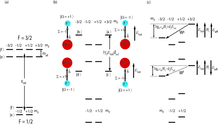
For Hunds’ case (a) molecular levels with , each rotational level is a -doublet, that is, it consists of two closely spaced levels of opposite parity. We can think of the even (odd) parity level as the symmetric (antisymmetric) superposition of the electronic angular momentum lying predominantly parallel and antiparallel to the molecular axis [Fig. 1(a)]. The parity doublet is split by the -doubling energy . A polar diatomic molecule will have a permanent electric dipole moment, , aligned along the internuclear axis , but in states of good parity, there will be vanishing expectation value in the lab frame. An applied laboratory electric field, , will act on to mix the states of good parity. In the limit of , energy eigenstates will have nonvanishing in the lab frame. More to the point, , a signed quantity given by the projection of the electron angular momentum on the molecular axis, , can also have a nonzero expectation value [Fig. 1(b)]. Heuristically, it is the large electric fields developed internal to the molecule, along , that gives rise to the large value of that the electron spin can experience in polar molecules. In the absence of the -doublet mechanism for polarizing the molecule, a much larger field would be necessary, , to mix rotational states with splitting typically twice the rotational constant . For HfF+, we estimate will be kHz, whereas will be about GHz. For a dipole moment D, mixing the -doublet levels will take a field well under 1 V/cm, whereas “brute force” mixing of rotational levels would require around 10 kV/cm. For an experiment on trapped ions, the smaller electric fields are essential.
In the context of their eEDM experiment on the level in PbO, DeMille and his colleagues have explored in some detail DeMille et al. (2000); Hunter et al. (2002); Kawall et al. (2004) the convenient features of an state, especially with respect to the suppression of systematic error. Our proposal liberally borrows from those ideas. In a molecule with at least one high-Z atom, states will be very similar to the state of PbO, but with typically smaller values of and much smaller values of magnetic g-factor. Singly charged molecules with spin triplet states will necessarily have an odd-Z atom, and thus the unavoidable complication of hyperfine structure, not present in PbO.
In Fig. 1 we present the , J = 1 state with hyperfine splitting due to the fluorine I=1/2 nucleus. A key feature is the existence of two near-identical pairs of -levels with opposite parity. As seen in Fig. 1(b), an external electric field, , mixes these opposite parity states to yield pairs of -levels with opposite sign of Kawall et al. (2004) relative to the external field. Fig. 1(c) shows the effect of a rotating magnetic bias field, parallel with the electric field, applied to break a degeneracy as described in Sec. IV.4 below. Note that any two levels connected by arrows in Fig. 1(c) transform into each other under time reversal. Time reversal takes , , and , where is the magnetic field. If we measure the resonant frequency for the transition indicated by the solid (or dashed) line once before and once after inverting the direction of the magnetic field, time reversal invariance tells us the difference between the two measurements should be zero. In the presence of an eEDM, which violates time-reversal invariance, this energy difference will give . As well, under the same magnetic field the transitions indicated by the solid and dashed lines should be degenerate, if the magnetic g-factors are identical for the states involved gfa . With non-zero eEDM the energy difference also gives .
Potential additional shifts, due predominantly to Berry’s phase Berry (1984), are discussed in Sec. IV but for now we note only that in the absence of new physics (such as a nonzero eEDM) the energy levels of a molecule in time-varying electromagnetic fields obey time-reversal symmetry. Reversing the direction of the electric field rotation while chopping the sign of the magnetic field amounts to cleanly reversing the direction of time, and will leave certain transition energies rigorously unchanged if . These are our “science transitions”, which we will measure with our highest precision.
II.5 Electronic Levels, Spin Preparation, and Spin Readout
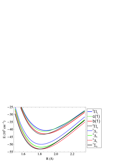
The density of trapped molecular ions will be too low to permit direct detection of the radio frequency or microwave science transitions. (A possible exception could involve the use of a superconducting microwave cavity, but this would add considerable experimental complexity.) We will of necessity rely on electronic transitions to prepare the initial electron spin state, and on a double resonance method to detect the spin flips. The details of these steps will depend on the specific molecule we use. For a qualitative illustration, we present a schematic of the calculated low-lying electronic potential curves of HfF+ (Fig. 2). We note that HfH+ and ThF+ have similar level structures Meyer et al. (2006); Petrov et al. (2007).
The molecules will be formed by laser ablation and cooled by supersonic expansion such that a large portion of the molecular population will be in ground state with a few rotational levels occupied (Sec. III.1). Spin-orbit mixing between states of identical are enhanced by relativistic effects in the high-Z Hf atom. The b(1) and c(1) states are well-mixed combinations of , and states, allowing for electric dipole transitions to and from these states that do not respect spin selection rules. The state, on the other hand, has no nearby state with which to mix, and thus and are good quantum numbers. Similarly, the state has so little contamination of in it that a rough calculation indicates that it is metastable against spontaneous decay, with a lifetime of order 300 ms Meyer et al. (2006); Petrov et al. (2007).
The Ramsey resonance experiment will begin with a two-photon, stimulated Raman pulse, off-resonant from the intermediate states, which will coherently transfer population from the ground state to the two magnetic sublevels of the level. The relative phase between the two magnetic levels evolves at a rate given by the energy difference. After a variable dwell time, a second Raman pulse is applied, which will coherently transfer a fraction of the population back down to the state, with probability determined by the accumulated relative phase. By varying the dwell time between Raman pulses, the population in the state will oscillate at a frequency given by the energy difference between the two spin states in the manifold.
The final step in the resonance experiment is to measure the number of molecules remaining in the state. This we propose to do with state-selective photodissociation. Molecules in the state will be dissociated via a two-color pulse, back up through the state to a repulsive curve, generating a Hf+ atomic ion and a neutral fluorine atom. Molecules in the state will not be affected by the two-color laser pulse and will remain as HfF+ molecular ions. The Paul trap parameters will be adjusted to confine only ions with the Hf+ atomic mass, and not the HfF+ molecular mass with mass difference amu. Finally, the potential on an endcap electrode will be lowered, and the remaining ions in the trap will be dumped onto a ion-counting device.
Details of this procedure will depend on the molecule ultimately selected for this experiment. We are also investigating alternative modes of spin state readout, including large-solid-angle collection of laser-induced fluorescence, and high finesse optical cavities Ye and Hall (2000).
III Experimental Apparatus
III.1 Molecular Beamline
We are interested in studying molecular radicals and therefore must create the molecules in situ. As described in Sec. II.2, we have a small collection of molecules that satisfy our selection criteria and our final choice of molecule has not been made. However, for clarity this section will describe the production, detection, and characterization of a beam containing neutral HfF molecules and HfF+ molecular ions.
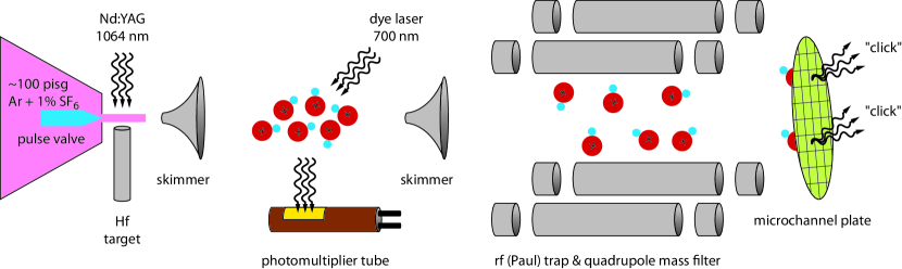
The molecules are made in a pulsed supersonic expansion (Fig. 3). A pulse valve isolates 7 atmospheres of argon that is seeded with 1% sulfur hexafluoride (SF6) gas from the vacuum chamber. The pulse valve opens for s allowing the Ar + 1% SF6 mixture to expand into the vacuum chamber. This creates a gas pulse moving at 550 m/s in the laboratory frame, but in the co-moving frame the expansion cools the translational temperature of the Ar atoms to a few Kelvin.
Immediately after entering the vacuum chamber, the gas pulse passes over a Hf metal surface. Neutral Hf atoms and Hf+ ions are ablated from this surface with a 50 mJ, 10 ns, 1064 nm Nd:YAG laser pulse. The ablation plume is entrained in the Ar + 1% SF6 gas pulse and the following exothermic chemical reactions occur:
| (1) | |||||
| (2) |
In the co-moving frame, the resulting neutral HfF molecules and HfF+ molecular ions are cooled through collisions with the Ar gas to rotational, vibrational, and translational temperatures of order a few Kelvin. The molecular beam then passes through a skimmer, first entering a region where laser induced fluorescence (LIF) spectroscopy is performed and finally arriving at an rf (Paul) trap where the ions are stopped and confined.
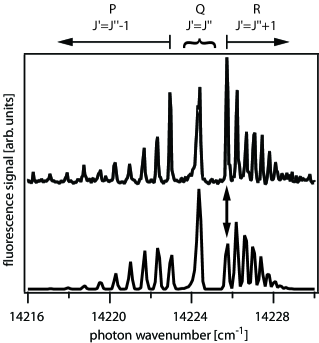
LIF spectroscopy is performed by transversely illuminating the molecular beam with a J, 10 ns, nm dye laser pulse. The linewidth of the dye laser is specified to be less than 0.1 cm-1. Fluorescence photons are collected and imaged onto a photomultiplier tube (PMT).
Using this technique we have found previously unobserved neutral HfF molecular transitions, one of which is shown in Fig. 4 (for previous neutral HfF spectroscopy see Ref. Adam et al. (2004)). The data shows that entrained neutral HfF molecules are cooled to rotational temperatures of order 5 K, with a large fraction of the population in the rotational ground state. We expect that entrained HfF+ molecular ions should be similarly cooled.
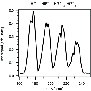
To detect the presence of HfF+ molecular ions in the beam the rf (Paul) trap is operated as a quadrupole mass filter. All of the ions in the beam are stopped and loaded into the trap. The voltages applied to the trap electrodes are then adjusted only to confine ions of a particular mass/charge ratio. Finally, the ions remaining in the trap are released onto the ion detector and counted. A typical mass spectrum is shown in Fig. 5, which clearly resolves the HfF+ molecular ions from the other atomic and molecular ions in the trap.
Our experimental count rate will be limited by space charge effects of the trapped ions. Therefore, any ions trapped that are not used in measuring the eEDM limit the statistical sensitivity of our measurement. In order to maximize our count rate, we wish to create and trap only HfF+ ions of a single Hf isotope and in a single internal quantum state. One scheme is to filter out all of the ions created from laser ablation and use photoionization techniques to ionize neutral HfF in as state-selective a way as possible. Using two color, two photon excitation, we excite to a high lying Rydberg state, in an excited vibrational level, that then undergoes vibrational autoionization Fie (b). The ion core of these Rydberg state molecules will occupy a single rotational level and consist of a single Hf isotope. The autoionization process is seen, in our preliminary (unpublished) data, to leave the ion core rotational level largely unperturbed. It should be possible to excite a Rydberg level that corresponds to an excited ion core with = 1, = 1 (where v is the vibrational quantum number). The Rydberg state might then vibrationally autoionize to the = 0, = 1 level that will be used to measure the eEDM.
III.2 Radio Frequency (Paul) Trap
For our preliminary studies of ion production, the ions are confined by a linear rf (Paul) trap shown schematically in Fig. 6. The ideal hyperbolic electrodes are replaced by cylinders of radius , where is the minimum radial separation between the trap center and the surface of the electrodes. This choice produces the best approximation to a perfect radial two-dimensional electric quadrupole field Denison (1971).
For HfF+ ( amu), an example set of operating parameters for the ion trap would be mm, mV, and kHz. This produces a ponderomotive potential that is well within the harmonic pseudo-potential approximation given by , where the radial secular frequency is approximately with . For the above parameters, , kHz, and K. Under these conditions, an ion cloud at a temperature of 15 K would have an rms radius of 5 mm. The trap can also be operated in mass filter mode Dawson (1995).
In addition to supplying the oscillating electric quadrupole field for radial confinement, the cylindrical electrodes can also be driven with voltages to produce the rotating electric bias field, , needed to polarize the molecular ions (Fig. 6). In order to generate neighboring electrodes will be driven out of phase at a frequency . The net voltage applied to each electrode is the sum of the voltages .
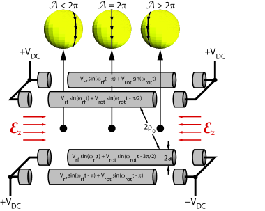
At present we are designing a second-generation ion trap with geometry designed for optimal precision eEDM spectroscopy, rather than for mass selection. The perfect ion trap would have very large optical access for collection of laser-induced fluorescence, and idealized electric and magnetic fields as follows
| (3) |
| (4) |
where and .
If we assume , that is not a rational fraction, and that , then we can cleanly separate out the ion motion into three components: rf micromotion, circular micromotion, and secular motion.
rf micromotion involves a rapid oscillation at whose amplitude grows as the ion’s secular trajectory takes it away from trap center. The kinetic energy of this motion, averaged over an rf cycle, is given by
| (5) |
where x and y in this case refer to the displacement of the ion’s secular motion.
The displacement of the ion’s circular micromotion is given by
| (6) |
The kinetic energy of the circular motion, averaged over a rotation cycle, is given by
| (7) |
The time-averaged kinetic energies of the two micromotions act as ponderomotive potentials that contribute to the potential that determines the relatively slowly varying secular motion:
| (8) |
In the idealized case, the secular motion corresponds to 3-d harmonic confinement with secular or “confining” frequencies
| (9) |
for . In the idealized case, confinement is cylindrically symmetric, , and is spatially uniform, so the circular micromotion does not contribute to the confining frequencies.
The density of ions will be low enough that there will be few momentum-changing collisions during a single measurement. Thus, any given ion’s trajectory will be well approximated by the simple sum of three contributions:
(i) a 3-d sinusoidal secular motion, specified by a magnitude and initial phase for each of the , , and directions. In a thermal ensemble of ions, the distribution of initial phases will be random and the magnitudes, Maxwell-Boltzmannian. For typical experimental parameters (see the Appendix) the secular frequencies will each be about kHz and the typical magnitude of motions, r, will be about 0.5 cm.
(ii) the more rapid, smaller amplitude rf micromotion, of characteristic frequency about kHz and radius perhaps 0.05 cm. This rf micromotion, purely in the x-y plane, is strongly modulated by the instantaneous displacement of the secular motion in the x-y plane, and vanishes at secular displacement x=y=0.
(iii) The still more rapid rotational micromotion, purely circular motion in the x-y plane, at frequency about kHz and of radius comparable to the rf motion, around 0.05 cm. In the idealized case, the rotational micromotion (in contrast to the rf micromotion) is not modulated by the secular motion.
As described in Secs. IV.5 and V below, for spectroscopic reasons we must operate with trapping parameters such that . Under that condition, relatively small imperfections in , say a spatial variation of , can give rise to contributions to of the same scale as the ions’ thermal energy, and thus significantly distort the shape of the trapped ion cloud or even deconfine the ions.
For improved optical access we had to shrink the radius of the linear electrodes with respect to their spacing The spectroscopic requirement for highly uniform then forced the redesign of the second-generation ion trap to be based on six near-linear elements arranged on a hexagon, rather the four electrodes arranged on square shown in Fig. 6. The trap will be discussed in more detail in a future publication, but simulations project spatial uniformity of better than with good optical access. The design led to significant compromises in the spatial uniformity of , so in future operation, mass selectivity in ion detection will come not from a quadrupole mass filter, but rather from pulsing to a very high value for a small fraction of a rotation cycle and then doing time-of-flight mass discrimination on the ions thus ejected. will be imposed by means of time-varying currents flowing lengthwise along the same electrodes that generate .
IV Spectroscopy in Rotating and Trapping Fields
On the face of it, an ion trap, with its inhomogeneous and rapidly time-varying electric fields, is not necessarily a promising environment in which to perform sub-Hertz spectroscopic measurements on a polar molecule. In this section we will explore in more detail the effects of the various components of the electric and magnetic fields on the transition energies relevant to our science goals. The theoretical determination of the energy levels of heavy diatomic molecules in the presence of time-varying electric and magnetic fields is a tremendously involved problem in relativistic few-body quantum mechanics. State-of-the-art ab initio molecular structure calculations are limited to an energy accuracy of perhaps Hz, a quantity which could be compared with the size of a hypothetical “science signal”, which could be on the order of Hz or smaller.
Fortunately, we can take advantage of the fact that at the energy scales of molecular physics, time-reversal invariance is an exact symmetry except to the extent that there is a time-violating moment associated with the electron (or nuclear) spin. In this section, except in those terms explicitly involving , we will assume that time-reversal invariance is a perfect symmetry in order to analyze how various laboratory effects can cause decoherence or systematic shifts in the relevant resonance measurements. The results can be compared to the size of the line shift that would arise from a given value of the electron EDM, which is treated theoretically as a very small first-order perturbation on the otherwise T-symmetric system.
In the subsections below, we bring in sequentially more realistic features of the trapping fields.
IV.1 Basic Molecular Structure
We begin by considering in detail the relevant molecular structure in zero electric and magnetic fields, thus quantifying the qualitative discussion of the experiment given in Sec. II. Although the molecular structure cannot be calculated in detail from ab initio structure calculations, nevertheless its analytic structure is well known. Because the measurements will take place in nominally a single electronic, vibrational, and rotational state, we will employ an effective Hamiltonian within this state, as elaborated by Brown and Carrington Brown and Carrington (2003). This approach will specify a few undetermined numerical coefficients, whose values can be approximated from perturbation theory, but which will ultimately be measured.
Brown Brown et al. (1987); Steimle et al. (1990); Nelis et al. (1991) and co-workers have done thorough work on deriving an effective Hamiltonian for molecules. The complete Hamiltonian in the absence of is given by
| (10) |
listed in rough order of decreasing magnitude. Since we are concerned only with terms acting within the subspace of the manifold, other electronic and vibrational states will enter only as perturbations that help to determine the effective Hamiltonian. Thus we consider eigenstates of and .
The remaining terms in Eq. (10) are corrections to the Born-Oppenheimer curves. They describe couplings between various angular momenta (, ), parity splittings (, ), and spin-dipolar interactions (, ). In typical Hund’s case (a) molecules these interactions are small compared to the rotational energy governed by . The relevant interactions that act within the manifold of states take the explicit form
| (11) | |||||
| (12) | |||||
| (13) | |||||
| (14) | |||||
| (15) | |||||
| (16) |
The constants in the first four terms are as follows: is the molecular spin-orbit constant, the rotational constant for the electronic level of interest, the effect of centrifugal distortion on rotation (typically , with the electron mass and the reduced mass of the molecule), governs the strength of the spin-spin dipolar interaction, and determines the strength of the interaction of the spin with the end-over-end rotation of the molecule. These four terms primarily describe an overall shift of the -level, and can be ignored in evaluating energy differences in the states we care about. They can, however, contribute small perturbations to these basic levels, as we will describe below.
Within the , manifold of interest, the energy levels are distinguished by the hyperfine and -doubling terms. The hyperfine Hamiltonian includes the familiar contact (), nuclear-spin-orbit () and spin-nuclear spin terms (). By estimating the parameters in perturbation theory, it is expected that the resulting hyperfine splitting is on the order of MHz Petrov et al. (2007). The hyperfine interaction also contains a previously unreported term, with constant denoted , that is connected to the -doubling. This term is expected to be even smaller than the already small -doublet splitting itself Mey , however, and will be ignored.
The -doubling Hamiltonian arises from Coriolis-type mixing of states with differing signs of due to end-over-end rotation of the molecule. For a state this interaction is characterized by three constants, of which the parameter is the dominant one. These terms describe how the state is perturbed by electronic states with and symmetry. Since we are primarily concerned with terms in the Hamiltonian that affect the ground rotational state of the electronic level, we only need to keep the term which connects to . This term has the general form, with numerical prefactors that depend on Clebsch-Gordon coefficients and wavefunction overlap, Brown et al. (1987)
| (17) |
where the sum is over all intermediate and states of singlet and triplet spin symmetries. For HfF+ this perturbation leads to a -doublet splitting on the order of kHz. This estimate was carried out assuming a molecular orbital configuration, where the orbital has total angular momentum in the pure precession approximation. The ground is a molecular orbital but has some admixture of atomic orbitals. We therefore expand the molecular wavefunction into atomic orbitals and reduce the amount of admixture by the factor that describes the character. From here on, we shall express the energy difference in parity levels for the as , rather than itself.
Thus the basic molecular structure of interest to the , state is governed by two constants: the hyperfine splitting (given by for ) and the -doublet splitting . These constants give the structure depicted in Fig. 1(a). These basic levels may be perturbed by couplings to other levels, especially rotational or electronic excited states. However, for the state of interest, some simplifications are possible, namely: (1) Off-diagonal couplings in are zero since preserves the value of J (there is no level with and ); (2) Off-diagonal contributions that mix into the manifold thus depend solely on the applied fields and the hyperfine interactions. Since the value of the spin-orbit constant is expected to be far larger than the rotational constant and we are concerned with a state, the operators that connect to will be ignored. The contributions to the ground state characteristics by terms off diagonal in are smaller by a factor of the hyperfine interaction energy to the spin-orbit separation energy, hence a factor of . This is the value which appears in front of any term connecting to in the ground state.
IV.2 Effect of Non-rotating Electric and Magnetic Fields
The influence of external fields presents new terms in the Hamiltonian of the form
| (18) | |||||
| (19) |
Here and are the electric and magnetic fields, assumed for the moment to be collinear so that they define the axis along which is a good quantum number; while and are the electric and magnetic dipole moments of the molecule.
The electric dipole moment arises from the body-fixed molecular dipole moment, at fields sufficiently small not to disturb the electronic structure. We assume that the field is sufficiently large to completely polarize this dipole moment, i.e., , in which case the Stark energies are given by
| (20) |
where is a geometric factor, analogous to a Landé g-factor, which accounts for the Stark effect in the total angular momentum basis . In the limit where the electric field is weak compared to rotational splittings, it is given by
| (21) |
Its numerical values in the state are therefore and . The electric field therefore raises the energy of the states with (denoted “upper” states with superscript ), and lowers the energy of states with (“lower” states with superscript ). This shift in energy levels is shown in Fig. 1(b), where and are upper and and are lower states.
The form of the Zeeman interaction is somewhat more elaborate, as the magnetic moment of the molecule can arise from any of the angular momenta , , , and . Quite generally, however, in the weak-field limit where , the Zeeman energies are given by , where is the Bohr magneton and are g-factors for the upper and lower states. In general, , and this difference can depend on electric field, a possible source of systematic error. We will discuss this in Sec. IV.7 below.
The leading order terms in the Zeeman energy are those that preserve the signed value of . They are given by
| (22) |
where is another Landé-type g-factor, but for nuclear spin. The orbital and spin g-factors are and , while the rotation and nuclear spin g-factors are and . Both and are small, being on the order of the electron-to-molecular mass ratio . Thus for an idealized molecule where , , , , we would expect molecular g-factors on the order of . More realistically, differs from 2 by a number on the order of , the fine structure constant, and a g-factor might be expected. In heavy-atom molecules such as ours for which spin-orbit effects mix , we may expect instead the difference to be as large as in magnitude. If we assume the dominant contribution comes from these spin-orbit type effects, we can define the -factor for the state as
| (23) |
while
| (24) |
Finally, the effect of the EDM itself introduces a small energy shift
| (25) |
where is the spin of the -electron contributing to the EDM signal; and denotes the intermolecular axis, with pointing from the more negative atom to the more positive one; in our case from the fluorine or hydrogen to thorium, platinum, or hafnium. Also in this convention we take as positive if it is anti-parallel to . The energy shift arising from this Hamiltonian depends only on the relative direction of the electron spin and the internuclear axis, and is given by
| (26) |
Polarizing the molecule in the external field selects a definite value of , hence a definite energy shift, positive or negative, due to the EDM. This additional shift is illustrated in Fig. 1(c).
For a range of field strengths and parameters, the energies of the sublevels within the manifold are well approximated by a linear expansion in the electric and magnetic fields. We define
| (27) |
Taking and , and setting , we get for the non-rotating energies,
| (28) |
where is either 1 or -1, and the prefactor in front of is such that for the level, - = = . and are good quantum numbers only to the extent that the electric field is neither too large nor too small, but we will use and as labels for levels even as these approximations begin to break down.
For notational compactness, we introduce special labels for particular states as follows (see Fig. 1(b)):
| (29) | |||||
with corresponding energies, , , , and , and identify the energies of two particularly interesting transitions, , and such that
| (30) |
Taking this analysis a step farther, it is possible that the electric field energy is not small compared to the hyperfine splitting . In this case the electric field mixes the different total- states and perturbs the above energies. Ignoring the magnetic field and EDM energies, the energy levels take the form
| (31) | |||||
| (32) | |||||
The equations of this section have so far been to one degree or another approximate results. But in the absence of exotic particle physics we can invoke time-reversal symmetry and write exact relations:
| (33) |
which, for , becomes
| (34) |
This exact degeneracy is, in fact, an example of the Kramers degeneracy that follows from time-reversal invariance Sachs (1987). For our purposes, the key result here is that, in the limit of non-rotating fields, zero applied magnetic field, and an electron EDM, the energy of the science transitions (and in particular, and ) are independent of the magnitude of the electric field. This is an important property because we are using spatially inhomogeneous electric fields to confine the ions in the trap, and we want to minimize the resulting decoherence.
This degeneracy in turn means that the energy differences and depend only on the magnetic field and, of course, the EDM term as shown in Eq. (30). The magnetic contribution reverses sign upon reversing the direction of with respect to the electric field direction (which also sets the quantization axis, since ). Therefore the science measurement is given by the combinations
| (35) |
where a sign on denotes that it points in the same direction as .
IV.3 Rotating Fields, Small-Angle Limit
Many EDM experiments over the years have been complicated by the problem of “Berry’s phase”, the term in this context used as a catch-all to describe a variety of effects related to the motion of the particles in inhomogeneous fields.
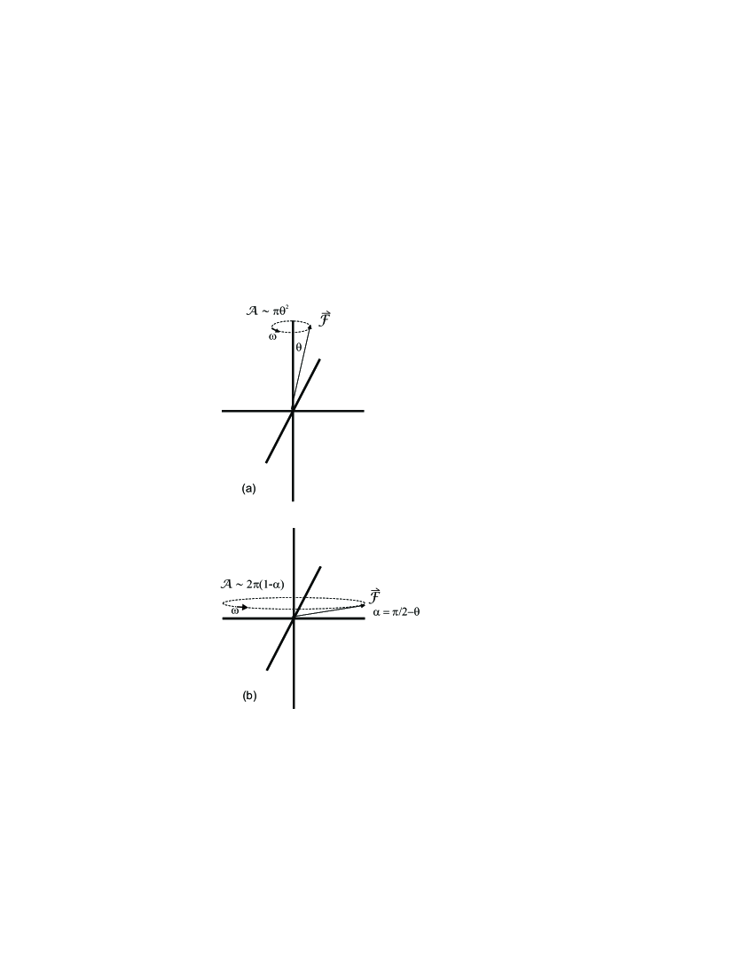
The sketch in Fig. 7(a) illustrates the classic Berry’s phase result: if the field that defines the quantization axis, as experienced locally by a particle (or atom, or molecule), precesses about the laboratory axis at some angle, , then, in the limit of slow precession, with each cycle of the precession the wave-function picks up a phase given by , where is the instantaneous projection of the particle’s total angular momentum on the quantization axis, and is the solid angle subtended by the cone. If the precession is periodic with period , one can (with provisos, as we will discuss) think of this phase-shift as being associated with a frequency, or indeed energy, . In a spectroscopic measurement of the energy difference between two states whose values differ by , there will be a contribution to the transition angular frequency .
In neutron EDM experiments, motional magnetic fields, in combination with uncharacterized fixed gradients from magnetic impurities, Berry’s phase can be a dangerous systematic whose dependence on applied fields can mimic an EDM signal Pendlebury et al. (2004). In Sec. IV.12 we will see that the effects of motional fields in our experiment are negligible.
Neutral atoms or molecules may be confined in traps consisting of static configurations of electric or magnetic fields. These traps are based on the interaction between the trapped species’ magnetic or electric dipoles and the inhomogeneous magnetic or electric fields, respectively, of the trap. Especially in cases where the traps are axially symmetric, so that the single-particle trajectory of an atom can orbit many times one way or the other about the axis of the trap, the coherence time of an ensemble of atoms with a thermal distribution of trajectories can be severely restricted Rupasinghe and Shafer-Ray (2008). Our system is quite different, because in an ion trap the forces arise from the interaction between the trapping fields and the monopole moment of our trapped ion. Assuming the temperature, size of bias field, and radius of confinement are the same, the trapping fields for an ion are spatially much more homogeneous than would be those for a neutral molecule or atom.
That said, the fact that we can speak of a “bias” electric field at all in an ion trap comes at the cost of having the applied electric field constantly rotating.
IV.4 Rotating Fields, Large-Angle Limit (Dressed States)
The basic dressed-state idea is an extension of the more common idea of an energy eigenstate: a system governed by a time-invariant Hamiltonian will have solutions such that for all and ; such a solution is called an energy eigenstate, with being then the corresponding energy. Similarly, a system governed by a periodic Hamiltonian with period such that for all values of , will have so-called “dressed-state” solutions such that for all and all integer values of . It is tempting to call the “energy” of the dressed state, but there will be an ambiguity in that energy because we can always replace with .
Operationally, the dressed state energies are derived from the eigenvalues of a formally time-independent Hamiltonian. If denotes the Hamiltonian in the absence of the field, then the appropriate rotation-dressed Hamiltonian is given by
| (36) |
is defined as Meyer et al. (2009)
| (37) |
where and are the projections of the total angular momentum into a set of axes where coincides with the instantaneous direction of the electric field. We now make explicit the rotating electric field with . The term thus provides an energy which, when multiplied by the rotational period , gives the ordinary Berry phase,
| (38) |
where we have taken the liberty of adding an arbitrary phase to reveal explicitly the solid angle .
In the experiment, the applied electric field should lie very nearly in the plane orthogonal to the rotation axis, i.e., . It is therefore useful to consider the small angular deviation from this plane, (Fig. 7). Then the apparent energy shift arising from the geometric phase is
| (39) |
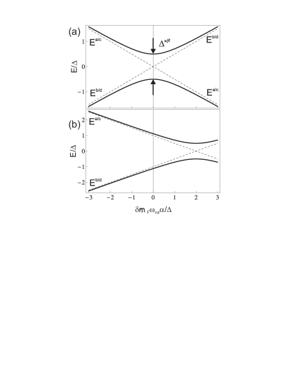
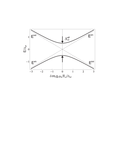
Now consider two states which are, in the absence of rotation, degenerate, say the states , with , and the state , with , indicated in Fig 1(b). Rotation breaks this degeneracy, by adding the energies , as shown by the dashed lines in Fig. 8. These levels cross at , leading to their apparent degeneracy when the electric field lies in the horizontal plane.
In addition, the rotation of the field also incurs coupling between states with different values, arising from the term in Eq. (37). This perturbation, treated at third-order in perturbation theory, connects the two levels and turns the crossing into an avoided one, as shown by the solid lines in Fig. 8. Since the energy contribution due to the rotating field is small compared to Stark energy splittings, we can use ideas similar to the derivation of -doubling, i.e., we take a sum of the perturbing components and take them to the appropriate power. We look for terms in this expansion that can connect the state to . Therefore, the power of perturbation theory needed is , where the takes and the extra power takes . The two terms in the Hamiltonian that can do this are the -doubling term and the -changing terms of the rotating electric field. Our expansion is, schematically, the following
| (40) |
The are the energy level differences between states with different values, thus are related to the Stark splittings. This tells us that
| (41) |
where is the energy splitting at the level crossing between otherwise degenerate states with and . The numerical prefactor in this expression has a rather complicated form within perturbation theory. However, its value can be computed by numerically diagonalizing the relevant hyperfine-plus-rotation dressed Hamiltonian Mey . The result, for the states in Fig. 1(b), is
| (42) |
where the superscript refers to mixing between the and states, and the superscript to mixing between and states. In the absence of the hyperfine interaction, the average value of the numerical prefactor is and the upper and lower states have the same avoided crossing. However, small fractional differences between and turn out to be significant, and are discussed further below.
The presence of the electric field causes the states with and to mix. Including the hyperfine interaction into the numerical diagonalization yields
| (43) | |||||
| (44) |
It is evident that the average shift is the same, but now the upper and lower levels acquire a different splitting due to the rotation-induced mixing within the sublevels. The difference is suppressed relative to the average value of the splitting by a factor of , reflecting the fact that higher orders of perturbation theory are needed to include the effects of the hyperfine interaction. For = 2 kHz, = 2 kHz, = MHz, = MHz, then = Hz and = Hz.
The magnitude of the rotation-induced mixing within any of the four pairs of otherwise degenerate states is much larger than the mixing within either pair of states, or . For this reason, the levels are probably not great candidates for precision metrology in rotating fields.
An ion in a trap will feel an axial force pushing it towards the axial position where the axial electric field vanishes, that is, the location at which is identically zero. This poses a problem, because at = 0, each dressed state is an equal mixture of states with and with . In other words, the dressed states right at the avoided crossing will have vanishing eEDM signal. The solution is to bias the avoided crossing away from by adding to the trapping fields a uniform, rotating magnetic field which is instantaneously always parallel or anti-parallel to vector ,
| (45) |
In our convention, defines the quantization axis, so that the number will always be taken to be positive. The sign of then determines whether the co-rotating magnetic field is parallel () or anti-parallel ().
The energy levels are now as shown in Fig. 8(b). As derived below in Sec. IV.5, in the limit , the dressed states near are once again states of good and . The energy splitting between the two states, as altered by the rotation of the field, are given approximately by
| (46) |
where the sign corresponds to states, and the sign to states.
Over the course of one axial oscillation of the ion in the trap, which is approximately proportional to the axial electric field, will average to zero. Unfortunately, the contributions to from and from are larger than that from the scale of the physics we most care about, , and the spatial and temporal variation in and in will reduce the coherence time of the spectroscopy, as discussed in Sec. IV.8 - IV.10 below. But to the extent that one is able quite precisely to chop to on alternate measurements, the science signal still arises from the same combination as in Eq. IV.2:
| (47) |
where the +/- corresponds to the superscripts respectively, and the brackets denote averaging over the excursions of , which is assumed to vary symmetrically about zero.
The equation above relies on several approximations. One needs in particular that , , and , , and . These are all good approximations, but they are not perfect. For example, using values from the Appendix, , a small number, but not zero. To what extent will imperfections in these approximations mimic an eEDM signal?
The driving principle of our experimental design is to measure with as close to a null background as possible. We are not especially concerned if the right hand side of Eq. (47) is 1.9 rather than 2.0 . More important to us is that, if , the right-hand side of Eq. (47) be as close to zero as possible. As we shall see, as long as we preserve certain symmetries of the system we are guaranteed a very high quality null. A preliminary remark is that the “energy” of a dressed state, or more precisely the phase shift per period , is unaffected by an offset in how the zero of time is defined. A second observation is that, in the absence of exotic particle physics (such as nonzero eEDM), the energy levels of a diatomic molecule in external electromagnetic fields are not affected by a global parity inversion.
Under the action of this inversion, all the fields and interactions in the Hamiltonian transform according to their classical prescriptions, whereas quantum states are transformed into their parity-related partners. In a parity-invariant system, parity thus changes quantum numbers, but leaves energies of the eigenstates unchanged. This is true for the dressed states as well, since their eigen-energies emerge formally from a time-independent Hamiltonian.
To formulate the effect of inversion symmetry we write the electric and magnetic fields as
| (48) | |||
| (49) |
where and . The dressed states defined by the rotating field are characterized by the projection of total angular momentum on the axis defined by the rotating electric field, . Because the magnetic field is not strictly collinear with the electric field, and because of the field rotation, is only approximately a good quantum number. Nevertheless, considering the effect of parity on all the ’s simultaneously, we can still map each dressed eigenstate into its parity-reversed partner.
Assuming the ions are “nailed down” in their axial oscillation, at a particular value of and thus , our various spectroscopic measurements would give dressed energy differences . Now we invoke the following symmetry argument: if we take the entire system, electric fields, magnetic field, and molecule, and apply a parity inversion, that will leave the energy of the corresponding levels unchanged. If further we then shift the zero of time by , in effect letting the system advance through half a cycle of the field rotation, that also will not change the corresponding energy levels of the dressed state, which are after all defined over an entire period of the rotation. This transformation effectively connects measurements made for , above the mid-plane, to those with , below the mid-plane. The combined transform acts as follows:
| (50) | |||||
The last of these is equivalent to , i.e., our symmetry operation would change the sign of the EDM energy shift. However, in the absence of this shift we can expect the following exact relations between the dressed state energies:
| (51) | |||
Summing four equations and rearranging terms, we get that
If we assume that the axial confinement is symmetric (not necessarily harmonic), and that our spectroscopy averages over an ensemble of ions oscillating in the axial motion with no preferred initial phase of the axial motion (we will later explore the consequences of relaxing this assumption) then the ions will spend the same amount of time on average at any given positive value of as they do at the corresponding negative value of , and thus the averaged results yield:
| (52) |
The combined result, in the absence of exotic particle physics, is zero by symmetry. We did not need to invoke the various approximations that went into Eq. 47. In particular, this null result is, unlike the traditional Berry’s phase result, not based on the assumption of very small . Also, for conceptual simplicity we have discussed the result as being based on an average over quasi-static values of , but the symmetry argument does not hinge on the axial frequency being infinitely slow compared to .
IV.5 Frequency- or Phase-Modulation of Axial Oscillation
The trapped ions will oscillate in the axial direction at a frequency , confined by an approximately harmonic axial trapping potential . Upon moving away from the mid-plane , the ions will experience an oscillating axial electric field . The geometric phase correction to the energy is then , where is the maximum excursion of the tilt angle. Because the product is again an energy, it is convenient to redefine the geometric energy contribution in terms of a frequency ,
| (53) |
with .
For kHz, an ion cloud temperature of 15 K, an ion whose axial energy is twice the thermal value, for and as shown in the Appendix, then a transition such as with will have a maximum frequency modulation Hz.
Thus the electric field at the ion’s location undergoes two motions, the comparatively fast radial rotation, and the comparatively slow axial wobble. We exploit the different time scales to create, for each instantaneous value of , the rotation-dressed states worked out in the previous section. The effect of the axial wobble is then described by the time variation of the amplitudes in these dressed states. The time-dependent Schrödinger equation of motion for this is
| (54) |
where and are the probability amplitudes for being in the and states, respectively. For typical experimental values, is about kHz, will range as high as kHz, and (given by Eq. 42) is perhaps Hz, and is about Hz.
Eq. 54 describes a system again governed by a periodic Hamiltonian, and we will therefore follow a similar course to Sec. IV.4 and search for dressed-state solutions such that . Of course, this will only be valid in the limit that , a necessary condition to write the time-dependent Hamiltonian in Eq. 54. First, we get rid of fast time-dependence by guessing solutions:
| (55) | |||
where are Bessel’s functions of the first kind and A(t) and B(t) are slowly varying functions. We then substitute our trial solutions into Eq. 54 and use the recurrence relation . We multiply through by or as appropriate. We then integrate over an axial time period, , and make the approximation that A(t) and B(t) are unchanged over this small time interval. This approximation should be good as long as and . The integration then yields,
| (56) |
with
| (57) |
This results in dressed-state energies, now as a function of , and not , as seen in Fig. 9. This clearly shows the requirement of in order to keep and as the dressed states. This is true despite the fact that an ion will sample the avoided crossing in Fig. 8 during its axial oscillation in the trap, as in our experiment. will have a maximum value of at and will oscillate about zero according to .
For finite , the dressed states from Eq. 56 only appear stationary if measured at integer multiples of the axial trapping period, . Consider states and , symmetric and antisymmetric combinations of states and , respectively. In the limit that , an ion initially in state will oscillate between and at the precession frequency , when measured at integer multiples of the axial trapping frequency. However, if our EDM measurement is made after a non-integer number of axial oscillations, or if the ions have different axial frequencies in the trap, the to oscillation will be frequency modulated at . For the example parameters, the frequency-modulation index is less than 1, and thus the spectral power of transition is overwhelmingly at , the quantity which symmetry arguments above show is unaffected by Berry’s phase. In an ensemble of ions which have a random distribution of initial axial motions, the sidebands on the transition average to zero, and won’t pull the frequency of the measured central transition. If instead the process of loading ions into the trap has left the ions with an initial nonzero axial velocity or axial offset from trap center, the measured frequency can be systematically pulled from .
We note that increasing or decreasing reduces the value of and thus the frequency modulation index. On the other hand, these changes also would have the effect of increasing the energy of the micromotion of the ions in the rotating fields. For harmonic axial confinement, we find the frequency modulation for a transition obeys the following relation . Thus to keep the modulation safely under unity for a comfortable majority of an ensemble of ions with an average given by , one needs to choose operating parameters such that . This inequality in turn places stringent requirements on the spatial uniformity of . On a time-scale slow compared to , acts like a sort of ponderomotive potential analogous to the effective confining potential in a Paul trap. If , then a spatial inhomogeneity in of only 1.5% already gives rise to structure in the ponderomotive potential comparable to .
To summarize the effect of axial motion: in the limit , ions prepared, for instance by optical pumping, in state (or ) will remain in (or ). The energy difference between dressed states which are predominantly either or will be slightly modified by the avoided crossing. But the important combined measurement described by Eq. (47) will continue to yield zero for = 0, and the sensitivity of that combined measurement to a nonzero EDM will not be much affected as long as .
IV.6 Structure of the Measurements. What Quantities Matter
In the remainder of this section, we will look at the possible effects of various experimental imperfections on our measurement.
The symmetry argument in Sec. IV.2 presupposes the ability to impose a perfect “-chop”, i.e., to collect data with alternating measurements changing quite precisely only the sign of . If not only the sign but the magnitude of the rotating magnetic field alternates, the situation is more complicated. There will likely be contributions to the rotating magnetic field that are not perfectly reversed in our -chop, including displacement currents associated with sinusoidally charging the electrodes that create the rotating electric field. These effects can be quantified with a value , and to lowest order they would appear as a frequency offset in the chopped measurement:
| (58) |
This offset is very nearly the same for the upper and lower states, to the extent that , i.e., to the extent that . The effect of the stray field is reduced by combining measurements from the upper and lower states, in the form of a “four-way chop”:
| (59) |
It may prove to be advantageous to shim the -chop by deliberately adding a non-chopped rotating magnetic field, , and adjusting its value until experimentally we measure
| (60) |
Then, a measurement in the lower -doublet state gives
| (61) |
yielding a still more accurate value for .
What we care about most then are: (1) Things that perturb and differently, in particular the quantity , but also the quantity , to be defined and estimated in Sec. IV.8, and (2) to a lesser extent, we care about effects which affect the same way as they affect , because, to the extent that they lead to a measurement
| (62) |
we can mistake a nonzero value for as an indicator for a nonzero value of . In that case, the shimming procedure discussed above to remove would lead to a combined result from the four-way chop of . This is down by a relative factor of compared to the effects that differentially perturb versus , but they could still be troublesome. And (3) to a still lesser extent, we care about imperfections that perturb individual measurements such as , even if they do not perturb the -chop measurement, , because, to the extent that they vary over time, or depend on the trajectory of an individual ion in the trap, they can reduce coherence times. This leads not to systematic errors, but to a reduction in the overall precision.
In addition to the chop, state chop, and four-way chop discussed above, we can perform a rotation chop, by changing the sign of . Our hope is to keep experimental imperfections to a level where the four-way chop is by itself already good enough to suppress systematic error below the desired level. Then repeating the entire series of measurements with the opposite sign of (rotating the field CW instead of CCW) will to the extent it yields the same final value of provide a useful redundant check.
IV.7 An Estimate of
There are two leading contributions to in our molecule. In the regime in which we will operate (a regime wherein is a signed quantity) they are to a good approximation independent of each other. These two contributions are the zero-field difference and the induced difference caused by the applied electric field. In the zero-field limit, the former is dominant. However, in the limit in which we are working, the latter dominates.
The zero electric field contribution arises due to centrifugal distortion effects in the molecular Hamiltonian. In Sec. IV.2, we wrote the Zeeman Hamiltonian in Eq. 22. We omitted two terms which connect states of . Therefore, these states will give rise to a parity dependent -factor for each -level. The Hamiltonians which govern this interaction can be found with the use of perturbation theory in a manner similar to the approach used to find the -doubling parameters. Brown et al. Brown et al. (1987) and Nelis et al. Nelis et al. (1991) have written these terms as
| (63) |
where is the centrifugal distortion induced by the magnetic field and is the Zeeman induced -doubling. is parity independent while is parity dependent. Due to the nature of the perturbation approach, we can estimate the size of in terms of the -doubling energy splitting
| (64) |
In addition, if the state of interest is composed of a molecular orbital (where and refer to atomic orbitals with ), then is expected. The difference in zero-field -factors is then given by twice the value in Eq. (64). It is evident that this effect is quite small, of the order for HfF+.
The electric field dependent -factor arises due to the mixing of rotational levels in the molecule. The levels with , while far away in energy compared to the Stark energy , are perturbers. In the signed basis, the sub-levels in the level have a smaller value than do the sub-levels in the level. Therefore, the states which go up (down) in energy in the level “gain” (“run”) on (from) the level. When one includes the effects of Hyperfine interactions, there are multiple connections to each sub-level. In the , levels that we are interested in, we can write an analytic expression for the electric field dependent factor
| (65) |
where . The terms in parentheses are -symbols while the term in curly brackets is a -symbol. The sum runs on all states connected to by the electric field. In the case of HfF+ with a ground state, the sum contains the and states. Since the rotation constant is far larger than either or , only is included in the perturbative expression for . For the parameters here, this contribution is
| (66) |
which means that the fractional shift is a few . The same approach gives that the electric field “g” factor, , will shift in the same manner such that .
For rotating fields, another contribution to arises from non-vanishing value of . The states with and are equally affected by the rotating field since they have an equal Stark shift in the absence of hyperfine interactions. However, because the levels with are repelled by the lower states, the effective Stark difference between levels with (upper levels) is smaller than the same levels with (lower levels). The scale at which this difference will appear is then determined by how much the lower hyperfine state pushes on the upper due to the coupling induced by the electric field.
| (67) |
This fractional shift is of the order a few and is therefore about the same magnitude as the electric field induced mixing of higher rotational levels.
IV.8 Dependencies on
Proximity to the avoided crossing shown in Fig. 8(b) means that the transitions and will have residual dependencies on , which in turn may lead to decoherence or systematic errors. We characterize the sensitivity of to small changes in with the following expansion
| (68) |
with
| (69) |
using the expressions in Eqs. (42) and (46). Any spatial inhomogeneity in that does not average away with ion motion will lead to a decoherence rate given approximately by .
In terms of systematic errors, if chopping the sign of gives rise to an unintended systematic change in the magnitude of (call it ), for instance due to motional fields discussed later, or due to ohmic voltages generated by the eddy currents, then there will be a frequency shift in a -chop combination, . To the extent that is nonzero, some of this shift will survive a four-way chop as well. The dominant contribution to is likely from , rather than from . Assuming this limit, the systematic error surviving is
| (70) |
For a large but not inconceivable value for of 100 V/cm, and for other values as in the Appendix, this works out to comfortably less than 100 Hz, and is therefore not a problem. But this error would scale as , and thus could cause trouble if for other reasons we chose to decrease . The science signal is roughly independent of , which should allow for the source of error to be readily identified.
IV.9 Perpendicular -Fields
The quantization axis is essentially defined by . The shift of the various levels , , , due to a component of the magnetic field perpendicular to is on the order of
| (71) |
for the upper/lower states. In the absence of rotation, the lowest-order correction to goes as
| (72) |
For reasonable experimental parameters, this will be a negligible number. The lowest-order correction to the state-chop combination, is smaller still and goes as
| (73) |
It is similar in form to the difference in -factors caused by the rotation of the field.
When we turn on rotation, there is an additional larger contribution to . If we assume (as a worst case) that is purely axial, not azimuthal, then the lowest-order effect of is to tilt the quantization axis by angle given by
| (74) |
with the +(-) in the numerator corresponding to the upper(lower) states and the +(-) in the denominator corresponding to the = -1(+1) states. This has the leading order effect on of
| (75) |
even a rudimentary nulling of the Earth’s magnetic field, say to below 25 mG, will leave this term negligible, for parameters in the Appendix. Its contribution to the state chop, , is still smaller by
| (76) |
IV.10 Stray Contributions to : Uniform or Time-Varying Fields
In the previous section we have seen that the effects of are small. Spatial or shot-to-shot variation in , on the other hand, can limit coherence time through its contribution to . The biggest contribution to is of course the intentionally applied rotating field . Let’s examine the various other contributions to .
Static, uniform fields: fields of this nature are relatively harmless. is defined relative to the quantization axis . The time-average of is . Since sweeps out a circle with angular velocity , the contribution to the time-averaged from a uniform, static magnetic field averages nearly to zero in a single rotation of the bias electric field, and still more accurately after a few cycles of axial and radial motion in the trap. The average electric field in the ion trap must be very close to zero, or the ions would not remain trapped. In the case of certain anharmonicities in the trapping potential, however, one can find that the average value of is nonzero, even if the average value of is zero. For instance, an electrostatic potential term proportional to , along with a uniform axial magnetic field , will for an ion with nonzero axial secular motion, yield a nonzero . In addition, nonzero will interact with the tilt of oscillating with an ion’s axial motion at to cause a frequency modulation similar to the one discussed in Sec. IV.5. A uniform magnetic field in the x-y plane will cause a frequency modulation at . If the modulation index for either of these modulations approaches one, the modulation will begin to suppress the contrast of spectroscopy performed at the carrier frequency. For uniform magnetic fields with amplitude less than 10 mG (achievable for instance by roughly nulling the earth’s field with Helmholtz coils), frequency modulation indices will be small, and, barring pathologically large electrostatic terms, the mean shifts from uniform, static fields will be less than 1 Hz and can be can be dealt with by means of an applied as discussed in Sec. IV.6.
Time-varying magnetic fields with frequency near can cause more trouble. If the time between the two Ramsey pulses used to interrogate the frequency is , then the dangerous bandwidth is , centered on . We discuss in order (i) thermally generated fields from the electrodes, (ii) ambient magnetic field noise in laboratory, (iii) magnetic fields associated with the application of , oscillating coherently with , (iv) shot to-shot variation in magnitude of applied , and (v) spatial inhomogeneities in .
(i) Proposed EDM experiments on trapped atomic species such as Cesium are vulnerable to magnetic field noise generated by thermally excited currents in conductors located close to the trapped species Munger (2005). In our case, the effect is less worrisome because, vis-a-vis the trapped atom experiments, our bandwidth of vulnerability is centered at much higher frequency fields, because our molecules are trapped considerably further from the nearest conductors, and because the sensitivity of our measurement of to magnetic field noise, which goes as is down by a factor of . The spectral density of thermal magnetic field noise (which is calculated in reference Henkel et al. (1999) in the simplified geometry of a semi-infinite planar conductor) will surely be less than 1 pG/Hz1/2 in our bandwidth of vulnerability. This effect is negligible.
(ii) Like thermal magnetic noise, technical magnetic noise in our lab arising for instance from various nearby equipment will not so much decohere an individual measurement as generate shot-to-shot irreproducibility between measurements. What level of noise are we sensitive to? As we discuss in Sec. VI below, the precision of a single trap load is unlikely to be better than 300 mHz, meaning magnetic field noise less than 0.2 G/Hz1/2 won’t hurt us, for a 1 s interrogation time. Measurements made in our lab show that there are a number of magnetic field “tones” of very narrow bandwidth, associated with harmonics of 60 Hz power and various power supplies. As long as we choose to not coincide with one of these frequencies, in the range of 50 kHz to 300 kHz ambient magnetic frequency noise in our lab has spectral density typically less than 0.02 G/Hz1/2. For this reason, at least for the first generation experiment, there will be no explicit effort to shield ambient magnetic field other than to use Helmholtz coils to roughly null the earth’s dc field. The steel vacuum chamber will in addition provide some shielding at 100 kHz.
(iii) In traditional eEDM experiments, one of the most difficult unwanted effects to characterize and bring under control is magnetic fields generated by leakage currents associated with the high voltages on the electrodes that generate the principal electric field. In our case the bulk of the electric field is generated inside the molecule. The laboratory electric fields are measured in V/cm, not kV/cm, and leakage currents as traditionally conceived will not be a problem for us. On the other hand, the electric field does rotate rapidly, and thus the electrode potentials must constantly oscillate. Displacement currents in the trapping volume between the electrodes, and real currents in the electrodes themselves and in the wire leads leading to them, will generate magnetic fields with spatial gradients and strengths that oscillate coherently with at the frequency .
The spatial structure of the oscillating magnetic fields will depend on the geometry of the electrodes and in particular on the layout of the wire leads that provide the current to charge them. In principle, shim coils can be constructed just outside the trap electrodes and driven with various phases and amplitude of current oscillating at , all in order to further control the shape of the magnetic field. The one immutable fact is the Maxwell equation, .
The dominant time dependence of the electric field is from the spatially uniform rotating field, and thus for a circular field trajectory, the dominant contribution to the magnetic field structure goes as
| (77) |
with
| (78) |
where is the direction in the x-y plane orthogonal to the instantaneous electric field.
The curl determines only the spatial derivatives of ; itself only depends on the boundary conditions. An idealized arrangement of current carrying leads and shim coils could in principle force the field to be
| (79) |
where is given by Eq. 78 and is displacement in the x-y plane along the direction of the instantaneous rotating electric field. These fields would be perpendicular to the quantization axis provided by the electric field, and would have negligible effect on the transitions of interest.
While realizing such an idealized displacement field would be very difficult, there are relatively simple steps to take to minimize the displacement fields. For instance, each rod-like electrode can be charged up by two leads, one connected to each end of the rod, with the leads running along respective paths symmetric in reflection in the z=0 plane to a common oscillating voltage source outside of the vacuum can, at z=0. It is worth considering a maximally bad electrode layout, to put a limit on worst-case performance. Our electrodes will be spaced by about 10 cm and mounted in such a way that their capacitance to each other or to ground will be at worst 5 pF. If the charging current is provided entirely by a single lead connected to one end of the rod, the peak current running down the rod near its center will be 80 A, leading to a worst-case field magnitude at the trap center of about 20 G, and a contribution to of perhaps 2.5 Hz. Spatial gradients of this effect, and shot-to-shot irreproducibility of this effect will not contribute to decoherence at the 0.1 Hz level. As for its contribution to systematic error, this shift will survive the -chop, but will be suppressed in the four-way chop by the factor , perhaps a factor of a thousand. For still better accuracy the shift should be nulled out of the chop by adjusting , as discussed in Sec. IV.6.
(iv)Given that the main effect of is to apply an offset frequency, of perhaps 8 Hz, and given that (see Sec. VI) the single-shot precision is unlikely to be any better than 300 mHz, the shot-to-shot reproducibility of need be no better than a part in 30, a very modest requirement on stability. Decoherence then is not a problem, but a potential source of systematic error arises if the the chop is not “clean” that is if before the chop is not exactly equal to after the chop. This sort of error could arise for instance from certain offset errors in op-amps generating the oscillating current. Experimentally, one adjusts to cancel these offsets, but even in the absence of that procedure, the four-way chop cleans up these sorts of errors. For a rather egregious fractional deviation from -chop cleanliness of, for instance, 1%, and for , the systematic error remaining after the four-way chop is of the offset frequency of perhaps 8 Hz. In HfF+ this is a systematic error on of e cm. For ThF+ the error as referred to is smaller still, and of course if we avail ourselves of so as to null the post -chop signal to 100 mHz, the systematic error on will be less than e cm for either species.
(v) The largest single contribution to decoherence (with the exception of spontaneous decay of the line to a lower electronic state) will likely be due to spatial inhomogeneity in the applied rotating bias field . That is to say, spatial inhomogeneities in that rotate in the x-y plane at frequency . First-order spatial gradients in are not important, because ion secular motion in the trap will average away the effects of these gradients leaving only the value of at the center of the trap. Second-order spatial gradients on the other hand will lead to nonzero average frequency shifts whose value will vary from ion to ion in a thermal sample of ions, depending on conserved quantities of individual ion motion like the axial secular energy Ez or radial secular energy Eρ, quantities with thermally averaged values of and , respectively, and with ion-to-ion variation comparable to their mean values. The will be generated by current-carrying rods which are of necessity within the vacuum chamber because of the screening effects of a metal vacuum chamber. Unless particular care is taken in the design of these rods, the second-order spatial gradients in will scale as , where is the characteristic size (and spacing) of the current carrying rods. The contribution to the inhomogeneity of the time-averaged value of experienced by a thermal sample of ions orbiting in a cloud with r.m.s size is then of order , leading to an ion-to-ion frequency variability of order For planned parameters of the experiment, is of order 0.01. We have seen from Sec. IV.5 above that the quantity must be at least about five times larger than in order to make the eigenstates in the rotating fields be states of good . Thus in the absence of explicit apparatus design to null the second-order spatial gradient in (The rod-like electrodes that bear the charge that generates are in the second-generation trap the same objects that carry the current that generates and thus their shape is already subject to multiple design constraints) we may have to live with a decoherence rate from this effect on the order of , perhaps 0.5 s-1, for the experimental values given in the Appendix.
The inhomogeneity in should reverse quite cleanly with the chop, and residual imperfections there will be cleaned up with the four-way chop, and thus the effects of the second-order gradients in are expected to be predominantly a source of decoherence, rather than systematic error on measured .
IV.11 Stray Contributions to : Static -Field Gradients
We now return to discussing static magnetic fields, now including the effects of spatial gradients. With the characteristic size of the ion cloud being smaller than the characteristic distance from cloud center to source of magnetic field by a ratio of 0.1 or smaller, it makes sense to expand the field about the uniform value at the trap center. The most general first-order correction to a static magnetic field in the absence of local sources can be characterized by five linearly independent components as follows:
| (80) | |||||
By far the most important effect of these terms is the “micromotion-axial gradient interaction.” As discussed in Sec. III.2 above, the displacement of an ion’s circular micromotion is exactly out of phase with the rotation of its quantization axis , see Eq. 6. Averaged over a cycle of , this will give rise to a nonzero average contribution to and cause a shift in given by . A guess for a possible value of stray is 2 mG/cm, which for anticipated experimental parameters would lead to a shift in of order 4 Hz, and this shift would survive the chop. As with the effect of displacement currents, one expects the systematic effect of the shift to be reduced after the four-way chop by , but for maximum accuracy the effect should be shimmed out of the chop, either by adjusting the value of , or by applying (say with anti-Helmholtz coils external to the vacuum chamber) a compensating value of .
A smaller effect arises from the interaction of the magnetic field gradient with the component of the electric fields responsible for providing ion confinement, which after averaging over cycles of and , always point inward, giving rise to a net inward-pointing time average of . If we look at only the component of the first-order magnetic field gradient that points towards or away from the trap center
| (81) |
The net contribution to comes from integrating, along the rf and rotation micromotion trajectories, over first a rotational cycle, and then an rf cycle, and then a secular cycle in a given direction. We assume that the trap is sufficiently harmonic that there is no cross-dimensional mixing of secular energy, that , , and are incommensurate and with principle axes as defined in Eq. 80, and that hard-momentum-changing collisions are rare enough so that, during the duration of a spectroscopic measurement, there is no change in , the sum of the kinetic and potential energy associated with an individual ion’s secular motion in the th direction. The contribution to is then,
| (82) |
The contribution to averaged over a thermal sample of ions is given by the above expression with replaced by . Note that for , several terms cancel and the thermally averaged contribution to is just . The decohering effect is comparable because within a thermal sample, , , and will in general differ from one another for a given ion, and between different ions. For and each about 2 mG/cm, ion temperatures about 15 K, the mean shift in Wu/ℓ for typical experimental parameters given in the Appendix might be 30 mHz, with a comparable contribution to dephasing.
The three remaining terms in the first-order gradient, , and , will contribute to a shift in only when combined with other (usually small) trap imperfections, for instance the plane of rotation of being tilted with respect to the principal axes of the confining potential. The net effects will be correspondingly smaller than those from .
Just as with the second spatial derivative of , the spatial derivative of , coupled to a thermal spread in the size of ion orbits, can give rise to decoherence. Of course, is defined already as a first spatial derivative of a magnetic field, thus the dephasing arises from a third derivative of the field, and its rate should be down from the mean size of the shift (roughly estimated above at 4 Hz) by a factor of order , or a factor of one hundred. Even spatially uniform could give rise to decoherence if there is a spatial dependence in . The fractional change in is the same as the fractional change in . As discussed in Sec. III.2, this should be smaller than 0.5% over the typical size of the ion sample.
As a coda to this subsection, it is worth considering that applying a very spatially uniform may be very challenging because of difficult-to-model eddy currents induced in electrodes and light-gathering mirrors. On the other hand a purposely applied static would be perturbed only by the magnetic permeability of trap construction materials, which can be minimized and modeled. One way or another we will need to bias away from the avoided crossing discussed in Sec. IV.4, but it may turn out that this can be accomplished with greater spatial uniformity and thus with a lower total decoherence rate by omitting the applied altogether, and providing the bias with a deliberately applied field. The chop could be accomplished by chopping the sign of . The parity invariance argument of Sec. IV.4 above can readily be modified to describe a chop of rather than a chop in .
To sum up subsections IV.J and IV.K, we have looked at a range of ways in which various contributions to can shift Wu and Wℓ. Decoherence due to shot-to-shot fluctuations or spatial inhomogeneity should not be a problem out to beyond 1 s coherence times. Various effects can shift Wu and Wℓ by as much as a few Hz, and this shift can survive a chop. With on order of 10-4, and estimated at 90 GV/cm in ThF+, after a four-way chop the remaining systematic error will be a few e cm, but this can be dramatically reduced by tuning away the post--chop signal with . The most dangerous systematic error would be if were systematically different between measurements on the upper and on the lower states. Chopping between upper and lower states will be determined by variations in optical pumping, which should be well decoupled from the mechanisms that generate .
IV.12 Relativistic (Ion-Motion-Induced) Fields
The largest component of the velocity on the ions is that of the micromotion induced by ; for reasonable experimental parameters it will be less than 1000 m/s. In typical lab-frame magnetic fields of a few mG, the motion will give rise, through relativistic transformation, to electric fields of order of a few V/cm, which are irrelevant to our measurement. Conversely, motion at 1000 m/s in typical lab-frame electric fields of 10 V/cm generates a magnetic field of 0.1 G. This field will be rigorously perpendicular to the electric field, the quantization axis, and thus represents only a negligible modification to the generally unimportant .
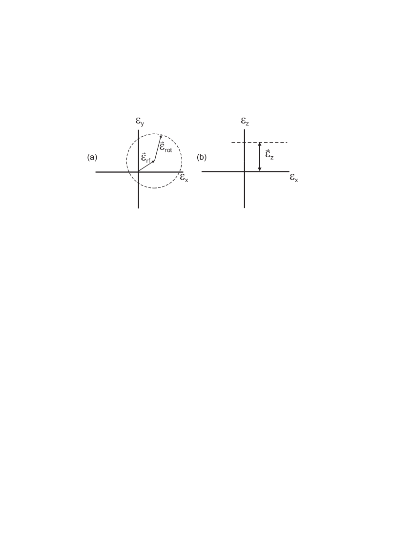
IV.13 Effect of RF Fields
The effects of the rf electric fields providing Paul trap confinement are best understood by putting them in the context of a three-tier hierarchy of electric field magnitudes and frequencies.
(i) , the nominally uniform, rotating electric field, with field magnitude of perhaps 5 V/cm and frequency kHz.
(ii) , the Paul-trap fields, are highly inhomogeneous, but at a typical displacement in the x-y plane of perhaps 0.5 cm, the field strength might be 75 mV/cm, or two orders of magnitude less than that of , oscillating at a frequency, kHz which is one order of magnitude less than . At a fixed point in space, the rf fields average rigorously to zero over time, but averaged instead along an ion’s rf micromotion trajectory, the rf fields contribute to
(iii) the inward-pointing trapping electric field, again very inhomogeneous but with typical strength down from peak rf-field values by factor of (/), another order of magnitude, to perhaps 5 mV/cm. From the ion’s perspective, the direction of the trapping fields oscillate with the ion’s secular motions in the trap, at frequencies of perhaps kHz, the slowest time scale by an order of magnitude.
The effects of the strong, fast have been discussed extensively throughout Sec. IV, and those of the weak, slow trapping fields were covered in Sec. IV.11 above. In this subsection we argue that the rf electric fields, intermediate in both frequency and strength, are the least significant of the three categories.
The effects of the rf fields averaged over the rf micromotion trajectory are discussed in Sec. IV.11. The remaining part averages to zero in one rf cycle, but is roughly frozen at a single value over the duration of one cycle of . The dominant source of the rf fields’ time-averaged contribution to transitions Wu/l is in very small corrections to Berry’s phase energy associated with the rotation of . See Fig. 10. The correction to the solid angle arising from Erf goes as (Ez/Erot)(Erf/Erot)2. If we include a factor of to get a Berry’s energy shift and evaluate for typical experimental parameters, the magnitude of the resulting frequency shift will be about 20 mHz, and will oscillate in sign with the axial secular motion. The magnitude of radial rf fields scales linearly with the radial secular displacement. If secular freqencies were commensurate, in particular if = 2, then this 20 mHz shift could contribute to a decoherence rate at the negligible level of a few tens of mHz. For incommensurate ratios of / or /, the rf fields will be still less important.
IV.14 Systematic Errors Associated with Trap Asymmetries
The symmetry argument of Sec. IV.4 was based on parity invariance. This argument is only as good as reflection symmetry of the electric and magnetic fields in the region of the trapped ions. In this section we look, as an example, at the consequences of a symmetry imperfection.
The electrodes used to generate have been numerically designed to make as spatially uniform as possible, but imperfections in design and construction of the trap and imperfect drive electronics will lead to some residual field nonuniformity. Suppose that the magnitude of the was consistently larger in the region of the trap for which z0, so that the value of over the z0 half of an axial secular oscillation is about 0.3% larger than that experienced over the z0 half. Thus the frequency modulation of perhaps 500 Hz, discussed in Sec. IV.5 will no longer average to precisely zero over an axial cycle but instead a net contribution of about 1.5 Hz to Wu. Such a frequency shift would survive a chop, and, following the protocol discussed in section IV.F, we could very likely incorrectly identify this shift as arising from the presence of a B, and apply a value of Bshim to largely null the 1.5 Hz shift. After a complete four-way chop, we would be left with a systematic error on the order of ()1.5 Hz, or about 0.4 mHz.
For the value of estimated for HfF+, a 0.4 mHz error corresponds to a systematic error on de of the order of a few e cm. For ThF+, the error on de would be about three times smaller. We continue a more general discussion on systematic errors in Sec. VI.4 below.
V Collisions
The overarching strategy of the trapped-ion approach to precision spectroscopy is to accept low count rates in exchange for very long coherence times. In some previous precision measurement experiments with trapped ions, the very best results have come from taking this to the extreme limit of working with only one ion Champenois et al. (2004); Matsubara et al. (2008); Chwalla et al. (2009); Margolis et al. (2004); Dube et al. (2005); Tamm et al. (2007); Hosaka et al. (2005); Oskay et al. (2006), or in some cases a pair of ions Chou et al. (2010), in the trap at any given time. More often however, optimal precision is achieved working with a small cloud of trapped ions. In this section we evaluate various detrimental effects of ion-ion interactions.
V.1 Mean-Field
With no electrons present to neutralize overall charge, even a relatively low density cloud of ions can have a significant mean-field potential. A spherically symmetric sample of ions confined within a sphere of radius will give rise to a mean-field potential
| (83) |
At values of the mean-field interaction energy comparable to or larger than , there is a risk of instabilities, viscous heating, and other undesirable effects; even in their absence, systematic errors are more difficult to analyze in the strong mean-field limit. Ion-trap experiments have been performed at much higher mean-field strengths, and indeed there have been precision spectroscopy experiments done in systems for which the interaction potential even between an individual pair of nearest-neighbor ions is much larger than . However, these systems exhibit a high degree of spontaneous symmetry breaking including crystallization Tan et al. (1995).
For the purpose of this paper, we assume the experiments will be done in the low mean-field limit, say
| (84) |
In this limit, mean-field effects are relatively benign, and can be modeled as a modest decrease in the trap confining frequencies, , plus the addition of some anharmonic terms to the potential. Crucially for the arguments presented in Sec. IV.4, these additional modifications do not break any of the reflection- or rotation-based symmetries of the trapping fields. We note that Eqs. 83 and 84 combine to set limits on various combinations of the ion number, , ion temperature, , cloud radii, , and mean ion density, . This necessitates making various compromises in selecting operating parameters.
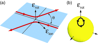
In Sec. IV.5, we saw that the axial component of the electric field at the ion’s location, , tilts the rotating electric field and gives rise to an apparent shift of the energy of our spectroscopic transition, linear in . This energy shift integrated over time in turn gives rise to an oscillatory phase shift, . In a one-component ion cloud, the effects of long-range, grazing-angle ion-ion collisions may be thought of as simply a fluctuating component to the local electric field, and the integrated effect of those fluctuations will make a random contribution to the phase shift. We present a simple argument to show that the resulting rms spread in phase does not continue to increase with time but reaches a steady-state asymptote. This is because not only shifts the transition energy, it also causes an axial force and corresponding acceleration, which, like the shift in transition energy, is linear in . Integrated over time, , this fluctuating force results in a fluctuating momentum. But we know that the combined effect of a trapping field and a large number of random collisions will not cause the rms momentum to randomly walk without bound but rather to be loosely bounded by a characteristic thermal value, . This is the nature of the thermal equilibration process – once an ion has developed a super-thermal momentum, further collisions are biased to reduce the momentum. Since both the phase excursion and the momentum excursion are linear in the time-integrated axial electric field, we can estimate . Again, as discussed in Sec. IV.5, if , the phase fluctuations for each ion’s spectroscopic transition will be bounded by a value less than one radian, so that there will be no loss in spectroscopic contrast in a Ramsey-type experiment.
The argument in the paragraph above hinges on the assumption that the electric field arising from the ion cloud’s mean-field distribution and from grazing-angle collisions is small in magnitude compared to , so that the shift in Berry energy is linear in the axial component of the electric field. For higher values of the ion temperature or lower values of , a pair of colliding ions can get so close to each other that the electric field is, transiently, comparable to or larger than . We discuss the consequences in the next subsection.
V.2 Geometric Phases Accumulated During an Ion-Ion Collision
As discussed in Sec. IV.4, when a spin adiabatically follows a time-varying quantization axis it acquires a geometric (Berry’s) phase. For the eigenstates in Fig. 1(b), the geometric phase factor can be written as , where is the solid angle subtended by the contour on the unit sphere traced out by the time-varying quantization axis. Thus, the relative phase generated between the states used for spectroscopy is . The concern of this subsection is how ion-ion collisions cause uncontrolled excursions of the quantization axis leading to random geometric phase shifts and decoherence between spin states. These uncontrolled phase shifts will be written as to distinguish them from the calibrated geometric phases in the experiment.
The instantaneous quantization axis for the molecular ion eigensates is defined by the net electric field vector at the location of the ion. During a collision, this axis is defined by the vector sum of the rotating electric field, , and the ion-ion interaction electric field, . Both of these are time-varying vectors, however typical ion-ion collisions have a duration short compared to the rotation period of so for the purpose of this discussion will be taken as stationary. Thus, the problem is reduced to calculating the excursion of the quantization axis under the time variation of . A typical ion-ion collision is shown in Fig. 11(a) and the effect of this collision on the quantization axis is shown in Fig. 11(b).
At the temperatures of our trapped ion samples, no two ions are ever close enough for the details of the intermolecular potential to matter. Only monopole-monopole and monopole-dipole interactions matter. Further, the translational degree of freedom may be treated as purely classical motion in a ion-ion potential, with the initial condition of a given collisional event characterized by an impact parameter and relative velocity. The outcome of the collision depends not only on the magnitudes of the impact parameter and of the velocity, but also on their angles with respect to the ambient electric bias field, . Each initial condition contributes a particular amount to the variance in the phase between the relevant internal states. These contributions can be converted to partial contributions to a decoherence rate, and a numerical integral over a thermal distribution of collisional initial conditions can yield the total decoherence rate. We have pursued this program to a greater or lesser extent with the decoherence mechanisms discussed in this subsection and the one immediately following, but the results are not especially illuminating and we have used them primarily to confirm that the power-law expressions discussed below represent only overestimates of the decoherence rate, and that for experimental parameters of interest, the decoherence rate will be conservatively less than 1 s-1.
The main question is whether is high enough to include significant phase space for collision trajectories for which the peak value of (which is to say, large enough to transiently tip the direction of the total field by more than a radian). If so, then a single collision can cause decoherence and one can get a simple estimate of the cross-section for decoherence simply from the size of the impact parameter that leads to those events. There is a significant probability for collisions with when
| (85) |
which leads to a decoherence rate
| (86) |
If is instead so low that the Coulomb barrier suppresses collisions that could lead to a sufficiently large value of and cause decoherence with a single collision, then decoherence will arise only from the combined effects of many collisions each causing small phase shifts that eventually random walk the science transition into decoherence. In this regime, the decoherence rate falls off very fast at low temperatures. For
| (87) |
typical collisions have and the decoherence rate is
| (88) |
Both Eqs. 86 and 88 represent conservative estimates of the decoherence rate, and for an intermediate range of temperature, the decoherence rate will be less than whichever estimate gives the smaller value (Fig. 12).
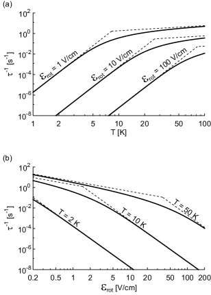
V.3 -Level Changing Collisions
A second source of decoherence can arise from ion-ion collisions that induce transitions between internal levels of a molecule. The dominant inelastic channel will be transitions between levels induced by a sufficiently sudden tilt in the quantization axis defined by the instantaneous local electric field. There are two conditions for such a transition to occur: (i) the direction of the total field must change by nearly a radian or more, so that there is significant amplitude for, e.g., an level in the unperturbed electric field to suddenly have non-negligible projection on an level in the collision-perturbed field, and (ii) the time rate of change of the electric field direction must be comparable to or larger than the energy splitting between an level and its nearest level in the field .
Note that the first requirement is the same as the requirement for picking up an appreciable single collision Berry’s phase. However, not all collisions that satisfy the first requirement will satisfy the second requirement. In particular, if the relative velocity in a collision is too low, then the time rate of change of the electric field direction will be too slow to satisfy the second requirement. Thus, given that the first requirement is satisfied, then the second requirement will not be satisfied when
| (89) |
In this limit, the second requirement is more stringent than the first requirement, which means that the rate of -level changing collisions will be smaller than the rate of single-collision Berry’s phase-induced decoherence. In the opposite limit, we expect the second requirement will be met whenever the first requirement is met, and thus we would expect that the two channels of decoherence, -level changing and single-collision Berry’s phase, will be comparable in magnitude.
Looking at particular collision trajectories in more detail, we see that there are trajectories that can cause an -level change but for which there is no contribution to Berry’s phase because the electric field traces out a trajectory with no solid angle (for instance, if the classical impact parameter is parallel to ). We also note that our formulation of the requirement of sweep rate for -level changing collisions neglects the fact that will not only change the direction of the total electric field () but also in general will change its magnitude. For most impact parameters, the magnitude of the total electric field will increase, thus suppressing nonadiabatic effects. However, a narrow range of impact parameters exists where the magnitude of the total electric field decreases, thus enhancing nonadiabatic effects. However, the above scaling laws account for the majority of collisions.
In the end, we are less interested in the actual rates than we are in putting conservative limits on decoherence rates. For instance, in calculating the curves in Fig. 12, we pessimistically took a worst-case geometry, , which gives an upper limit on the size of the effect. Thus we estimate that:
-
•
For the total collisional decoherence, including both -level-changing and Berry’s-inducing effects, will be less than or equal to the value given by solid curves in Fig. 12, while
-
•
For , the total collisional decoherence will be no greater than twice as large as the rate indicated by those curves.
VI Conclusions: Precision and Accuracy
Recall from Sec. I the three components to the sensitivity figure-of-merit:
VI.1 Coherence Time
Conclusions of Sec. IV and V: Taking into account only collisional decoherence, and all the questions associated with being in rotating fields and in trapping fields, we would anticipate a coherence time longer than one second. Black-body thermal excitation of the J=1 rotational level will also be well over one second. Vibrational black-body excitation for the v=0 state is estimated at 6 s for HfF+ in a 300 K environment. Thus the dominant limitation to coherence will likely be the radiative lifetime of the state, estimated Petrov et al. (2009) at 390 ms for HfF+, and still longer for ThF+, for which the state is predicted to be still lower in energy. The largest uncertainty in the lifetime calculation is the uncertainty in the decay energy, calculated to be 1600 cm-1 in HfF+.
VI.2
in HfF+ is calculated by Meyer and coworkers to be 30 GV/cm Meyer and Bohn (2008), and by Titov et al. to be 24 GV/cm Petrov et al. (2007). For ThF+, Meyer calculates 90 GV/cm Meyer and Bohn (2008). The uncertainties in these numbers are hard to assess, but they are very likely accurate to better than a factor of two and, if ongoing spectroscopic studies provide experimental values of hyperfine and fine structure that confirm the ab initio values predicted by the St. Petersburg group, our confidence in the precision of calculated will be much higher.
VI.3 Count Rate and Summary of Expected Precision
We are producing HfF+ ions by photoionization in a relatively narrow range of quantum states, and can estimate yield per quantum level within the desired trapping volume at perhaps 100 ions per shot, but we have just begun to characterize the efficiency of the process and very little optimization has been done. Our design efficiency for reading out spin states of trapped ions via laser-induced fluorescence (LIF) is 4%, but that has not been verified yet. With a large uncertainty, then, we may detect about one ion per shot with four shots per second. Overall, precision in one hour could be about 10 mHz. For ten hours of data, we anticipate (very roughly) a raw precision at e cm in HfF+, and e cm in ThF+. We are investigating several more efficient alternatives to LIF for spin readout, including in particular resonantly enhanced photodissociation or second photoionization. Even if we detect as many as four ions in a shot, single shot precision will be no better than 300 mHz, which sets a relaxed requirement for suppressing experimental shot-to-shot noise.
VI.4 Accuracy, Systematic Error
We have not completed a systematic study of the consequences of all possible violations of reflection symmetry in the trapping fields, but work in this direction is ongoing.
For now, we make the following three observations:
i) For the field asymmetries we have analyzed to date, realistic estimates for the magnitude in as-constructed field imperfections lead to systematic errors on the order of a few 10-29 e cm or less. While this is not yet as accurate as our ultimate ambitions, it would represent roughly a factor of thirty improvement on the existing best experimental limit.
ii) Asymmetries analyzed to date lead to systematic errors whose signs reverse when the direction of rotation reverses. If we combine measurements made with clockwise and counterclockwise field rotation, the errors vanish. Ideally, we’d like to design sufficient accuracy into the experiment so that the chop in field rotation is not needed to achieve desired accuracy, but as a practical matter we will of course run the experiment both ways, averaging the results to get ultimate accuracy, and differencing them to diagnose experimental flaws.
iii) Auxiliary measurements are envisioned to characterize and shim out flaws in the as-constructed trap. For instance, we plan to be able to shim the equilibrium position of the ion cloud up and down along the trap axis, and at each location measure the energy difference Eb-Ed. Unlike Ea-Eb, Eb-Ed is highly electric-field sensitive. The result will be a precise measurement of any spatial gradient in .
iv) All systematic errors we have analyzed to date have strong dependencies on quantities such as , , , and on the ion-cloud temperature and density, and the trap confining frequencies. A true signal from a nonzero value of de will be largely independent of all those quantities. We anticipate making a number of auxiliary measurements with the experimental parameters tuned far away from their optimal values to deliberately exaggerate the size of systematic errors and allow us thus to characterize their dependencies in less integration time than that required for ultimate sensitivity. Even so, and as is often the case in precision measurement experiments, sensitivity and accuracy are coupled. To the extent we can measure de to high precision at many combinations of experimental parameters, we will better be able to detect and reject false signals.
We believe the experiment as we have described it should have the capability to improve the limit on the electron’s electric dipole moment to 10-29 e cm. As of this writing, the largest contribution to the uncertainty in our ultimate capability has to do with unknown efficiencies of state preparation and read out. More specialized publications from our group addressing progress in these areas are forthcoming.
VI.5 Summary
Until now, molecular ions have not been viable candidates for symmetry violation searches largely due to the fact that applying electromagnetic fields to manipulate the internal states of the molecule would also violently perturb the translational motion of the ions. In this work, we have proposed a technique to overcome this obstacle – namely applying an electric field that rotates at radio frequencies. The specifics of performing high-resolution electron spin resonance spectroscopy under these conditions were analyzed. In particular, we have shown that a significant advance towards detecting the permanent electric dipole moment of the electron can be made by probing the valence electrons in a ground or metastable level of an ensemble of trapped diatomic molecular ions.
Note added in proof: Since the submission of this work, a new experimental limit on the electric dipole moment of the electron has been achieved using YbF molecules: e cm Hudson et al. (2011).
Appendix: Typical Experimental Parameter Values
mHz, transition energy between and states in ThF+ if = 1.7 x 10⁻²⁹ e cm.
= +1.50 a.u. MHz/(V/cm), electric dipole moment of HfF+ in the molecular rest frame.
= 5 V/cm, rotating electric field.
kHz, frequency of rotating electric field.
K, typical kinetic energy in rotational micromotion.
= 0.6 mm, radius of circular micromotion.
MHz.
(3/2) MHz, Stark shift of states of levels in rotating electric field.
kHz, -doublet splitting between opposite parity J=1 states.
, magnetic g-factor in states.
= 70 G, rotating magnetic field.
Hz, Zeeman splitting between and states due to .
/ 3 10-4, fractional difference of magnetic g-factor for upper and lower levels, for parameters shown in the Appendix.
Hz, splitting at the avoided crossing between = +3/2 and = -3/2 levels, for parameters shown in the Appendix.
mG, anticipated scale of transverse magnetic field.
r = 0.5 cm, characteristic rms radius of trapped ion cloud.
T = 15 K, characteristic temperature of trapped cloud.
kHz, typical trap confining frequency.
mV/cm, typical axial electric field applied for confinement.
mV/cm, typical Paul trap electric field strength, at typical cloud radius.
= 5 mV/cm, typical radial confining electric field, averaged over one Paul cycle.
kHz, typical “rf freq” for Paul trap.
K, typical kinetic energy in Paul micromotion.
MHz, hyperfine splitting between F = 1/2 and F = 3/2 states of J=1 level.
Acknowledgments
We gratefully acknowledge many useful discussions. On the topic of molecular and atomic spectroscopy, we benefited from discussions with Peter Bernath, Carl Wieman, Tom Gallagher, Ulrich Hechtfische, and Jim Lawler. On molecular structure, Andrei Derevianko, Svetlana Kotochigova, Richard Saykally, Laura Gagliardi, and especially the St. Petersburg group, Anatoly Titov, Mikhail Kozlov, and Alexander Petrov. On molecular dynamics, we had useful discussions with Carl Lineberger, David Nesbitt, and especially Bob Field. On EDM measurements, Pat Sandars, Dave DeMille, and Neil Shafer-Ray. We thank Gianfraco DiLonardo for the loan of a hollow cathode lamp and Tobin Munsat for the loan of a high-current power supply. We acknowledge useful contributions in our lab from Herbert Looser, Tyler Yahn, Tyler Coffey, Matt Grau, and Will Ames. We thank Jun Ye and members of his group for sharing their innovative ideas in comb-based spectroscopy, and Konrad Lehnert for enlightening us about sensitive microwave detection. This work was supported by NIST, NSF, and funds from a Marsico Chair of Excellence.
References
- Commins and Bucksbaum (1983) E. D. Commins and P. H. Bucksbaum, Weak interactions of leptons and quarks (Cambridge University Press, 1983).
- Wood et al. (1997) C. S. Wood, S. C. Bennett, D. Cho, B. P. Masterson, J. L. Roberts, C. E. Tanner, and C. E. Wieman, Science 275, 1759 (1997).
- Guéna et al. (2005) J. Guéna, M. Lintz, and M.-B. Bouchiat, Mod. Phys. Lett. 20, 375 (2005).
- Tsigutkin et al. (2009) K. Tsigutkin, D. Dounas-Frazer, A. Family, J. E. Stalnaker, V. V. Yashchuk, and D. Budker, Phys. Rev. Lett. 103, 071601 (2009).
- Crassous et al. (2005) J. Crassous, C. Chardonnet, T. Saue, and P. Schwerdtfeger, Org. Biomol. Chem. 3, 2218 (2005).
- Quack et al. (2008) M. Quack, J. Stohner, and M. Willeke, Annu. Rev. Phys. Chem. 59, 741 (2008).
- Hegstrom et al. (1980) R. A. Hegstrom, D. W. Rein, and P. G. H. Sandars, J. Chem. Phys. 73, 2329 (1980).
- Harris (2002) R. A. Harris, Chem. Phys. Lett. 365, 343 (2002).
- DeMille et al. (2008a) D. DeMille, S. B. Cahn, D. Murphree, D. A. Rahmlow, and M. G. Kozlov, Phys. Rev. Lett. 100, 023003 (2008a).
- Isaev et al. (2010) T. A. Isaev, S. Hoekstra, and R. Berger, Phys. Rev. A 82, 052521 (2010).
- Flambaum and Kozlov (2007) V. V. Flambaum and M. G. Kozlov, Phys. Rev. Lett. 99, 150801 (2007).
- Zelevinsky et al. (2008) T. Zelevinsky, S. Kotochigova, and J. Ye, Phys. Rev. Lett. 100, 043201 (2008).
- DeMille et al. (2008b) D. DeMille, S. Sainis, J. Sage, T. Bergeman, S. Kotochigova, and E. Tiesinga, Phys. Rev. Lett. 100, 043202 (2008b).
- Kajita and Moriwaki (2009) M. Kajita and Y. Moriwaki, J. Phys. B 42, 154022 (2009).
- Bakalov et al. (2010) D. Bakalov, V. Korobov, and S. Schiller, Phys. Rev. A 82, 055401 (2010).
- Hudson et al. (2006) E. R. Hudson, H. J. Lewandowski, B. C. Sawyer, and J. Ye, Phys. Rev. Lett. 96, 143004 (2006).
- DeMille et al. (2000) D. DeMille et al., Phys. Rev. A 61, 052507 (2000).
- Hunter et al. (2002) L. R. Hunter et al., Phys. Rev. A 65, 030501 (2002).
- Kawall et al. (2004) D. Kawall, F. Bay, S. Bickman, Y. Jiang, and D. DeMille, Phys. Rev. Lett. 92, 133007 (2004).
- Kozlov and DeMille (2002) M. G. Kozlov and D. DeMille, Phys. Rev. Lett. 89, 133001 (2002).
- Petrov et al. (2005) A. N. Petrov, A. V. Titov, T. A. Isaev, N. S. Mosyagin, and D. DeMille, Phys. Rev. A 72, 022505 (2005).
- Hudson et al. (2002) J. J. Hudson, B. E. Sauer, M. R. Tarbutt, and E. A. Hinds, Phys. Rev. Lett. 89, 023003 (2002).
- Sauer et al. (2006) B. E. Sauer, H. T. Ashworth, J. J. Hudson, M. R. Tarbutt, and E. A. Hinds, Atomic Physics 20, 44 (2006).
- Shafer-Ray (2006) N. E. Shafer-Ray, Phys. Rev. A 73, 034102 (2006).
- Kozlov et al. (1987) M. G. Kozlov, V. I. Fomichev, Y. Y. Dmitriev, L. N. Labzovsky, and A. V. Titov, J. Phys. B 20, 4939 (1987).
- Dmitriev et al. (1992) Y. Y. Dmitriev et al., Phys. Lett. A 167, 280 (1992).
- Vutha et al. (2010) A. C. Vutha et al., J. Phys. B 43, 074007 (2010).
- Meyer and Bohn (2008) E. R. Meyer and J. L. Bohn, Phys. Rev. A 78, 010502(R) (2008).
- Lee et al. (2009) J. Lee, E. R. Meyer, R. Paudel, J. L. Bohn, and A. E. Leanhardt, J. Mod. Opt. 56, 2005 (2009).
- Meyer et al. (2006) E. R. Meyer, J. L. Bohn, and M. P. Deskevich, Phys. Rev. A 73, 062108 (2006).
- Rainville et al. (2005) S. Rainville, J. K. Thompson, E. G. Meyers, J. M. Brown, M. S. Dewey, E. G. Kessler Jr., R. D. Deslattes, H. G. Börner, M. Jentschel, P. Mutti, et al., Nature 438, 1096 (2005).
- Gabrielse (2006) G. Gabrielse, Int. J. Mass Spect. 251, 273 (2006).
- Odom et al. (2006) B. Odom, D. Hanneke, B. D’Urso, and G. Gabrielse, Phys. Rev. Lett. 97, 030801 (2006).
- Gabrielse et al. (2006) G. Gabrielse, D. Hanneke, T. Kinoshita, M. Nio, and B. Odom, Phys. Rev. Lett. 97, 030802 (2006).
- Schwalm (2007) D. Schwalm, Prog. Part. Nucl. Phys. 59, 156 (2007).
- Roth et al. (2006) R. Roth, P. Blythe, H. Daerr, L. Patacchini, and S. Schiller, J. Phys. B 39, S1241 (2006).
- Roueff and Herbst (2009) E. Roueff and E. Herbst, J. Phys.: Conf. Ser. 192, 012008 (2009).
- Willitsch et al. (2008) S. Willitsch, M. T. Bell, A. D. Gingell, and T. P. Softley, Phys. Chem. Chem. Phys. 10, 7200 (2008).
- Staanum et al. (2010) P. F. Staanum, K. Højbjerre, P. S. Skyt, A. K. Hansen, and M. Drewsen, Nat. Phys. 6, 271 (2010).
- Schneider et al. (2010) T. Schneider, B. Roth, H. Duncker, I. Ernsting, and S. Schiller, Nat. Phys. 6, 275 (2010).
- Tong et al. (2010) X. Tong, A. H. Winney, and S. Willitsch, Phys. Rev. Lett. 105, 143001 (2010).
- Svendsen et al. (2010) A. Svendsen, U. J. Lorenz, O. V. Boyarkin, and T. R. Rizzo, Rev. Sci. Instrum. 81, 073107 (2010).
- Chen et al. (2011) K. Chen, S. J. Schowalter, S. Kotochigova, A. Petrov, W. G. Rellergert, S. T. Sullivan, and E. R. Hudson, Phys. Rev. A 83, 030501 (2011).
- Sandars (1967) P. G. H. Sandars, Phys. Rev. Lett. 19, 1396 (1967).
- Sandars (1975) P. G. H. Sandars, Atomic Physics 4, 71 (1975).
- Cho et al. (1989) D. Cho, K. Sangster, and E. A. Hinds, Phys. Rev. Lett. 63, 2559 (1989).
- Khriplovich (1998) I. B. Khriplovich, Phys. Lett. B 444, 98 (1998).
- Farley et al. (2004) F. J. M. Farley et al., Phys. Rev. Lett. 93, 052001 (2004).
- Orlov et al. (2006) Y. F. Orlov, W. M. Morse, and Y. K. Semertzidis, Phys. Rev. Lett. 96, 214802 (2006).
- Oshima (2010) S. Oshima, Phys. Rev. C 81, 038501 (2010).
- Adelmann et al. (2010) A. Adelmann et al., J. Phys. G 37, 085001 (2010).
- Bennett et al. (2009) G. W. Bennett et al., Phys. Rev. D 80, 052008 (2009).
- Bennett et al. (2002) G. W. Bennett et al., Phys. Rev. Lett. 89, 101804 (2002).
- Bennett et al. (2004) G. W. Bennett et al., Phys. Rev. Lett. 92, 161802 (2004).
- Hughes and Kinoshita (1999) V. W. Hughes and T. Kinoshita, Rev. Mod. Phys. 71, S133 (1999).
- Pospelov and Khriplovich (1991) M. E. Pospelov and I. B. Khriplovich, Sov. J. Nucl. Phys. 53, 638 (1991).
- Bernreuther and Suzuki (1991) W. Bernreuther and M. Suzuki, Rev. Mod. Phys. 63, 313 (1991).
- Barr (1993) S. M. Barr, Int. J. Mod. Phys. A 8, 209 (1993).
- Pospelov and Ritz (2005) M. Pospelov and A. Ritz, Ann. Phys. 318, 119 (2005).
- Regan et al. (2002) B. C. Regan, E. D. Commins, C. J. Schmidt, and D. DeMille, Phys. Rev. Lett. 88, 071805 (2002).
- Commins et al. (1994) E. D. Commins, S. B. Ross, D. DeMille, and B. C. Regan, Phys. Rev. A 50, 2960 (1994).
- Ramsey-Musolf and Su (2008) M. J. Ramsey-Musolf and S. Su, Phys. Rep. 456, 1 (2008).
- Chupp (2009) T. Chupp, Nucl. Phys. A 827, 428C (2009).
- Jungmann (2007) K. Jungmann, arXiv:hep-ex/0703031v1 (2007).
- Ritz (2009) A. Ritz, Nucl. Instrum. Methods 611, 117 (2009).
- Paul (2009) S. Paul, Nucl. Phys. A 827, 414C (2009).
- Wilschut et al. (2010) H. W. Wilschut et al., Nucl. Phys. A 844, 143C (2010).
- Abdallah et al. (2004) J. Abdallah et al., Eur. Phys. J. C 35, 159 (2004).
- Baker et al. (2006) C. A. Baker et al., Phys. Rev. Lett. 97, 131801 (2006).
- Ban et al. (2006) G. Ban et al., Hyperfine Interact. 172, 41 (2006).
- (71) SNS Neutron EDM Experiment, http://p25ext.lanl.gov/edm/edm.html.
- Onderwater (2006) C. J. G. Onderwater, Nucl. Phys. B – Proc. Sup. 155, 375 (2006).
- Griffith et al. (2009) W. C. Griffith et al., Phys. Rev. Lett. 102, 101601 (2009).
- Yoshimi et al. (2008) A. Yoshimi et al., Hyperfine Interact. 181, 111 (2008).
- Rosenberry and Chupp (2001) M. A. Rosenberry and T. E. Chupp, Phys. Rev. Lett. 86, 22 (2001).
- Ledbetter et al. (2005) M. P. Ledbetter, I. M. Savukov, and M. V. Romalis, Phys. Rev. Lett. 94, 060801 (2005).
- Fie (a) P. Fierlinger (private communication).
- Tardiff et al. (2008) E. R. Tardiff et al., Phys. Rev. C 77, 052501 (2008).
- Pandey et al. (2010) K. Pandey et al., Phys. Rev. A 81, 033424 (2010).
- Shidling et al. (2009) P. D. Shidling et al., Nucl. Instr. Meth. Phys. Res., Sect. A 606, 305 (2009).
- Guest et al. (2007) J. R. Guest et al., Phys. Rev. Lett. 98, 093001 (2007).
- Holt et al. (2010) R. J. Holt et al., Nucl. Phys. A 844, 53C (2010).
- Dzuba et al. (2009) V. A. Dzuba, V. V. Flambaum, and S. G. Porsev, Phys. Rev. A 80, 032120 (2009).
- Abdullah et al. (1990) K. Abdullah, C. Carlberg, E. D. Commins, H. Gould, and S. B. Ross, Phys. Rev. Lett. 65, 2347 (1990).
- (85) Energies will be quoted as angular frequencies, in radians/second, or temperatures, in Kelvin, where the factors of and are omitted from equations, respectively.
- Sandars (1965) P. G. H. Sandars, Phys. Lett. 14, 194 (1965).
- Sandars (1966) P. G. H. Sandars, Phys. Lett. 2, 290 (1966).
- Liu and Kelly (1992) Z. W. Liu and H. P. Kelly, Phys. Rev. A 45, R4210 (1992).
- Hartley et al. (1990) A. C. Hartley, E. Lindroth, and A. M. Martensson-Pendrill, J. Phys. B 23, 3417 (1990).
- Amini et al. (2007) J. M. Amini, C. T. Munger, and H. Gould, Phys. Rev. A 75, 063416 (2007).
- Fang and Weiss (2009) F. Fang and D. S. Weiss, Opt. Lett. 34, 169 (2009).
- (92) D. Heinzen (private communication).
- Murthy et al. (1989) S. A. Murthy, D. Krause Jr., Z. L. Li, and L. R. Hunter, Phys. Rev. Lett. 63, 965 (1989).
- Kozlov and Ezhov (1994) M. G. Kozlov and V. F. Ezhov, Phys. Rev. A 49, 4502 (1994).
- Titov et al. (1996) A. V. Titov, N. S. Mosyagin, and V. F. Ezhov, Phys. Rev. Lett. 77, 5346 (1996).
- Kozlov (1997) M. G. Kozlov, J. Phys. B 30, L607 (1997).
- Quiney et al. (1998) H. M. Quiney, H. Skaane, and I. P. Grant, J. Phys. B 31, L85 (1998).
- Parpia (1998) F. A. Parpia, J. Phys. B 31, 1409 (1998).
- Mosyagin et al. (1998) N. S. Mosyagin, M. G. Kozlov, and A. V. Titov, J. Phys. B 31, L763 (1998).
- Isaev et al. (2004) T. A. Isaev et al., Phys. Rev. A 69, 030501 (2004).
- Petrov et al. (2007) A. N. Petrov, N. S. Mosyagin, T. A. Isaev, and A. V. Titov, Phys. Rev. A 76, 030501 (2007).
- Tarbutt et al. (2004) M. R. Tarbutt et al., Phys. Rev. Lett. 92, 173002 (2004).
- Lamoreaux (2002) S. K. Lamoreaux, Phys. Rev. A 66, 022109 (2002).
- Heidenreich et al. (2005) B. J. Heidenreich et al., Phys. Rev. Lett. 95, 253004 (2005).
- Budker et al. (2006) D. Budker, S. K. Lamoreaux, A. O. Sushkov, and O. P. Sushkov, Phys. Rev. A 73, 022107 (2006).
- Liu and Lamoreaux (2004) C. Y. Liu and S. K. Lamoreaux, Mod. Phys. Lett. A 19, 1235 (2004).
- Player and Sandars (1970) M. A. Player and P. G. H. Sandars, J. Phys. B 3, 1620 (1970).
- Dzuba et al. (2000) V. A. Dzuba, V. V. Flambaum, and J. S. M. Ginges, Phys. Rev. A 61, 062509 (2000).
- (109) This is a good approximation at the level.
- Berry (1984) M. V. Berry, Proc. R. Soc. Lond. A 392, 45 (1984).
- Ye and Hall (2000) J. Ye and J. L. Hall, Phys. Rev. A 61, 061802 (2000).
- Adam et al. (2004) A. G. Adam, W. S. Hopkins, and D. W. Tokaryk, J. Mol. Spec. 225, 1 (2004).
- Fie (b) R.W. Field (private communication).
- Paul (1990) W. Paul, Rev. Mod. Phys. 62, 531 (1990).
- Denison (1971) D. R. Denison, J. Vac. Sci. Technol. 8, 266 (1971).
- Dawson (1995) P. H. Dawson, editor, Quadrupole Mass Spectrometry and Its Aplications (American Institute of Physics, 1995).
- Brown and Carrington (2003) J. Brown and A. Carrington, Rotational Spectroscopy of Diatomic Molecules (Cambridge University Press, 2003).
- Brown et al. (1987) J. M. Brown, A. S.-C. Cheung, and A. J. Merer, J. Mol. Spec. 124, 464 (1987).
- Steimle et al. (1990) T. C. Steimle, D. F. Nachman, J. E. Shirley, D. A. Fletcher, and J. M. Brown, Mol. Phys. 69, 923 (1990).
- Nelis et al. (1991) T. Nelis, S. P. Beaton, K. M. Evenson, and J. M. Brown, J. Mol. Spec. 148, 462 (1991).
- (121) E. R. Meyer, Ph.D. thesis, JILA, 2010.
- Sachs (1987) R. Sachs, The Physics of Time Reversal (Chicago Press, 1987).
- Pendlebury et al. (2004) J. M. Pendlebury et al., Phys. Rev. A 70, 032102 (2004).
- Rupasinghe and Shafer-Ray (2008) M. Rupasinghe and N. E. Shafer-Ray, Phys. Rev. A 78, 033427 (2008).
- Meyer et al. (2009) E. R. Meyer, A. Leanhardt, E. Cornell, and J. L. Bohn, Phys. Rev. A 80, 062110 (2009).
- Munger (2005) C. T. Munger, Phys. Rev. A 72, 12506 (2005).
- Henkel et al. (1999) C. Henkel, S. Potting, and M. Wilkens, Appl. Phys. B 69, 379 (1999).
- Champenois et al. (2004) C. Champenois et al., Phys. Lett. A 331, 298 (2004).
- Matsubara et al. (2008) K. Matsubara et al., Appl. Phys. Express 1, 067011 (2008).
- Chwalla et al. (2009) M. Chwalla et al., Phys. Rev. Lett. 102, 023002 (2009).
- Margolis et al. (2004) H. S. Margolis et al., Science 306, 1355 (2004).
- Dube et al. (2005) P. Dube et al., Phys. Rev. Lett. 95, 033001 (2005).
- Tamm et al. (2007) C. Tamm et al., IEEE Trans. Instrum. Meas. 56, 601 (2007).
- Hosaka et al. (2005) K. Hosaka et al., IEEE Trans. Instrum. Meas. 54, 759 (2005).
- Oskay et al. (2006) W. H. Oskay et al., Phys. Rev. Lett. 97, 020801 (2006).
- Chou et al. (2010) C. W. Chou, D. B. Hume, J. C. J. Koelemeij, D. J. Wineland, and T. Rosenband, Phys. Rev. Lett. 104, 070802 (2010).
- Tan et al. (1995) J. N. Tan, J. J. Bollinger, B. Jelenkovic, and D. J. Wineland, Phys. Rev. Lett. 75, 4198 (1995).
- Petrov et al. (2009) A. N. Petrov, N. S. Mosyagin, and A. V. Titov, Phys. Rev. A 79, 012505 (2009).
- Hudson et al. (2011) J. J. Hudson, D. M. Kara, I. J. Smallman, B. E. Sauer, M. R. Tarbutt, and E. A. Hinds, Nature 473, 493 (2011).